TIFR/TH/98-01 January, 1998 hep-ph/9801240

Quarkonium Polarization in Non-relativistic QCD
and the Quark-Gluon Plasma

Sourendu Gupta

Theory Group, Tata Institute of Fundamental Research,

Homi Bhabha Road, Bombay 400005, India.

We examine angular distributions of leptons arising from the decay of $J/\psi$ in inclusive hadroproduction. Taking into account feed-down contributions from $\chi_{1,2}$, a flat distribution emerges without fine tuning parameters. Changes in the ratio of direct to total $J/\psi$ cross sections would change this distribution significantly. Such angular distributions are, therefore, confirmatory tests of the $J/\psi$ suppression signal for the production of a quark-gluon plasma. Related effects are predicted for the $\Upsilon$.

1 Introduction

In the hadroproduction of $J/\psi$, the angular distribution of the dileptons coming from the decay of the quarkonium is of the form

$${d\sigma\over d\cos\theta}\;\sim\;1+\alpha\cos^{2}\theta$$ (1.1)

where $\theta$ is the angle (measured in the rest frame of the quarkonium) between the direction of motion of the positively charged lepton and the (lab-frame) direction of the quarkonium momentum. As long as the initial particles are unpolarized, there can be no difference in the weights for production of quarkonia with helicities $m$ and $-m$. The angular distributions can then be summarized by an “alignment parameter” [1]—

$$\zeta\;=\;{\sigma_{L}\over\sigma},\qquad{\rm and}\qquad\alpha\;=\;{1-3\zeta\over 1+\zeta}.$$ (1.2)

Here $\sigma_{L}$ is the cross section for production of quarkonia with longitudinal polarization ($J_{z}=0$), and $\sigma$ is the total cross section. For hadroproduction, $\alpha$ is close to zero for all beam and target combinations investigated [2, 3], implying that $\zeta$ is close to $1/3$.

The question of angular distributions and alignment has attracted a lot of attention recently. In [4] it was pointed out that heavy-quark spin symmetry has strong implications for $\zeta$. Non-relativistic QCD (NRQCD) [5], which incorporates heavy-quark spin symmetry, is a framework for understanding production rates of quarkonia. Polarization in hadroproduction has been investigated in NRQCD in [6, 7, 8]. The dependence of $\alpha$ on kinematics is claimed to be a discriminant between different models for hadroproduction of quarkonia, and hence a crucial test of NRQCD [9]. Polarization of quarkonia produced in the decay of $Z_{0}$ has also been investigated [10], and may be tested at LEP.

The phenomenological application of NRQCD to inclusive hadroproduction of $J/\psi$ has been quite successful. Absolute cross sections are fully compatible with the scaling laws of NRQCD, and the energy dependence of total cross sections [6, 11], as well as longitudinal momentum distributions [12] are reproduced rather well. The ratio of $\chi_{1}$ and $\chi_{2}$ cross sections can also be understood by going to higher than leading orders in the NRQCD expansion parameter, $v$ [13]. In view of this, the alignment of quarkonia produced in inclusive hadron-hadron collisions is investigated. Although the computations are performed to leading order in $v^{2}$ for each channel, this already leads to an expansion to order $v^{9}$ in some cases.

Our results are summarized here. The observation of almost vanishing $\alpha$ in inclusive $J/\psi$ production arises from the mixture of direct $J/\psi$ and feed-down from $\chi$ states. We compute alignments in NRQCD at sufficiently high order, thus supplementing the results of [7, 8] by formulæ for $\zeta_{\chi}$. The value of $\alpha$ depends only on the ratios of certain non-perturbative matrix elements, and is well constrained by the scaling laws of NRQCD. A flat angular distribution emerges because of the feed-down from $\chi$ states.

This has implications for the $J/\psi$ suppression signal of the quark-gluon plasma [14]. A plasma melts not only the $J/\psi$, the more massive quarkonium states are disrupted even more easily— indeed it has been speculated that some of them dissolve even at temperatures lower than the QCD phase transition [15]. If this is so, then a suppression of the $J/\psi$ cross section due to a plasma must be coupled with a large change in $\alpha$. This provides a confirmatory test for the $J/\psi$ suppression signal of the formation of a quark-gluon plasma in relativistic heavy-ion collisions.

In section 2 the computation of the angular distribution in NRQCD is outlined in brief. Details of the computation are given in appendix A, where a helicity technique used in conjunction with previously known methods of computation is documented. In section 3 the results for $\zeta$ are summarized. In the final section 4 these results are applied to inclusive hadroproduction and the signal of quark-gluon plasma formation.

2 Non-relativistic QCD

NRQCD is a low-energy effective theory for quarkonia [5]. The action is written in terms of all possible operators consistent with the symmetries of QCD. All momenta in NRQCD are cut off by some scale $\Lambda$, taken to be of the order of the heavy quark mass, $m$. The coupling associated with each term is identified through a perturbative matching procedure. In NRQCD the perturbative short-distance ($<1/\Lambda$) physics of the production of a heavy quark pair ($\bar{Q}Q$) is factored from the non-perturbative long-distance physics of its hadronisation to a quarkonium. A proof of factorisation has been given for production at large transverse momenta [5] and successful phenomenology has been done [16]. An explicit test of factorisation for inclusive cross sections is provided by a recent next-to-leading order, $\alpha_{\scriptscriptstyle S}^{2}$, computation [17].

The NRQCD factorisation formula for the inclusive production of heavy quarkonium resonances $H$ with 4-momentum $P$ can be written as

$$d\sigma\;=\;{\displaystyle{1\over\Phi}{d^{3}P\over(2\pi)^{3}2E_{\scriptscriptstyle P}}}\sum_{ij}C_{ij}\left\langle{\cal K}_{i}\Pi(H){\cal K}^{\dagger}_{j}\right\rangle,$$ (2.1)

where $\Phi$ is a flux factor. The coefficient functions $C_{ij}$ are computable in perturbative QCD and hence have an expansion in the strong coupling $\alpha_{\scriptscriptstyle S}/\pi$ (evaluated at $\Lambda$). Although each matrix element in the sum above is non-perturbative, it has a fixed scaling dimension in the quark velocity $v$. Then the NRQCD cross section is a double series in $\alpha_{\scriptscriptstyle S}/\pi$ and $v^{2}$. For charmonium a numerical coincidence, $\alpha_{\scriptscriptstyle S}/\pi<v^{2}$, makes it necessary to consider higher orders in $v^{2}$ before going to higher orders in $\alpha_{\scriptscriptstyle S}$.

The fermion bilinear operators ${\cal K}_{i}$ are built out of heavy quark fields sandwiching colour and spin matrices and the covariant derivative ${\bf D}$. The composite labels $i$ and $j$ include the colour index $\alpha$, the spin quantum number $S$, the number of derivative operators $N$, the orbital angular momentum $L$, the total angular momentum $J$, the helicity $J_{z}$ and the parity. The hadron projection operator

$$\Pi(H)\;=\;{\sum_{s}}\left|H,s\rangle\langle H,s\right|,$$ (2.2)

(where $s$ denotes hadron states with energy less than the NRQCD cutoff), is diagonal in appropriate bases [4, 5, 7]. When the final state helicities are summed it is diagonal in $J$, $J_{z}$ and parity. When the hadron helicity is observed, heavy quark spin symmetry makes it diagonal (up to corrections of order $v^{2}$) in the basis $\{S,L,J_{z}\}$.

The $J_{z}$-dependence of these matrix elements can be factored out using the Wigner-Eckart theorem—

$$\begin{array}[]{rl}&\langle{\cal K}_{i}\Pi(H){\cal K}^{\dagger}_{i}\rangle\;=\;{\displaystyle{1\over\hat{J}^{2}}}{\cal O}^{H}_{\alpha}({}^{2S+1}L_{J}^{N}),\\ &\langle{\cal K}_{i}\Pi(H){\cal K}^{\dagger}_{j}\rangle+{\rm h.c.}\;=\;{\displaystyle{1\over\hat{J}\hat{J}^{\prime}}}{\cal P}^{H}_{\alpha}({}^{2S+1}L_{J}^{N},{}^{2S+1}L_{J^{\prime}}^{N^{\prime}}).\end{array}$$ (2.3)

The factors of $\hat{J}=\sqrt{2J+1}$ come from Clebsch-Gordan coefficients and are conventionally included in the coefficient function. NRQCD supports a power counting rule for each matrix element—

$$\langle{\cal K}_{i}\Pi(H){\cal K}^{\dagger}_{j}\rangle\;=\;R_{H}\Lambda^{D}v^{d},$$ (2.4)

where $D$ is the mass dimension of the operator, and the NRQCD order, $d$, is given by the rule

$$d\;=\;3+N+N^{\prime}+2(E_{d}+2M_{d}).$$ (2.5)

$E_{d}$ and $M_{d}$ are the number of colour electric and magnetic transitions required to connect the hadronic state to the state ${\cal K}_{i}|0\rangle$. At tree level the dimensionless number $R_{H}$ in eq. (2.4) must depend only on the hadron $H$ under consideration. At higher orders in $\alpha_{\scriptscriptstyle S}$, $R_{H}$ may be corrected by logarithms of $\Lambda$.

Matrix Elements	Values	$R_{H}$
${\cal O}^{J/\psi}_{8}\left({}^{3}S_{1}\right)$	$(1.12\pm 0.14)\times 10^{-2}{\rm\ GeV}^{3}$	$0.22\pm 0.03$
${\cal O}^{J/\psi}_{8}\left({}^{1}S_{0}\right)+{7\over 2m^{2}}{\cal O}^{J/\psi}_{8}\left({}^{3}P_{0}\right)$	$(3.90\pm 1.14)\times 10^{-2}{\rm\ GeV}^{3}$	$0.17\pm 0.05$
${\cal O}^{\psi^{\prime}}_{8}\left({}^{3}S_{1}\right)$	$(0.46\pm 0.08)\times 10^{-2}{\rm\ GeV}^{3}$	$0.09\pm 0.02$
${\cal O}^{\psi^{\prime}}_{8}\left({}^{1}S_{0}\right)+{7\over 2m^{2}}{\cal O}^{\psi^{\prime}}_{8}\left({}^{3}P_{0}\right)$	$(1.60\pm 0.51)\times 10^{-2}{\rm\ GeV}^{3}$	$0.07\pm 0.02$

Table 1: The values of various non-perturbative matrix elements in the non-relativistic normalisation [18]. These can be converted to the relativistic normalisation by multiplying by $4m$. The dimensionless number $R_{H}$ (eq. 2.4) has been extracted using $\Lambda=m=1.5$ GeV and $v^{2}=0.3$.

In principle, we would like to do phenomenology with experimental measurements of the matrix elements needed. However, the large number of different matrix elements required for fixed target phenomena makes this impossible at present. Consequently, we are forced to use the scaling laws of eq. (2.4). Any number obtained in this way can at best be indicative, and has to be justified by more detailed numerical work when better data becomes available. The first step is, of course, to test eq. (2.4). From the data summarized in Table 1 it seems that tree-level NRQCD scaling can be accepted as a working hypothesis.

The coefficient functions, $C_{ij}$, are computed using a non-relativistic decomposition of heavy quark spinors and a Taylor expansion of the matrix elements, $\cal M$, in the relative momentum, $q$, of the $\bar{Q}Q$ pair [8]. Spherical tensor techniques are then used to recouple the 2-component spinor bilinear operators [13]. The projection to specific $J_{z}$ components can be performed at the matrix element level by appropriate choice of gauge. The process of matching the perturbatively computed $|{\cal M}|^{2}$ to the NRQCD formula of eq. (2.1) is then simple.

3 Quarkonium alignment

We need to compute the alignment parameter only for $J/\psi$, $\chi_{1}$ and $\chi_{2}$. For completeness, we also list it for the yet unestablished ${}^{1}P_{1}$ state $h_{c}$. A simple extension of the results in [8] is sufficient to show that $\zeta^{H}_{\bar{q}q}=0$ for all quarkonia $H$ to all orders in $v$. The total cross section has been listed in [13] to order $\alpha_{\scriptscriptstyle S}^{2}v^{9}$. In this section only the longitudinal parts of the $gg\to\bar{Q}Q$ cross sections are listed. Some details are given in Appendix A.

3.1 Direct $J/\psi$ alignment

The direct $J/\psi$ subprocess longitudinal cross section is

$$\hat{\sigma}^{J/\psi}_{gg}(\hat{s})\;=\;\varphi\left[{5\over 144}\theta^{J/\psi}_{D}(7)+\left\{{5\over 144}\theta^{J/\psi}_{D}(9)+{1\over 16}\theta^{J/\psi}_{F}(9)\right\}\right]$$ (3.1)

where

$$\varphi={\pi^{3}\alpha_{s}^{2}\over 4m^{2}}\delta(\hat{s}-4m^{2}),$$ (3.2)

and $\theta^{J/\psi}_{a}(n)$ denotes combinations of non-perturbative matrix elements from the colour amplitude $a$ ($=S$, $D$ or $F$) at order $v^{n}$. These can be written as

$$\begin{array}[]{rl}\theta^{J/\psi}_{D}(7)\;=&{\displaystyle{1\over 2m^{2}}}{\cal O}^{J/\psi}_{8}({}^{1}S_{0}^{0})+{\displaystyle{3\over 2m^{4}}}{\cal O}^{J/\psi}_{8}({}^{3}P_{0}^{1})\\ \theta^{J/\psi}_{D}(9)\;=&-{\displaystyle{23\over 8\sqrt{3}m^{4}}}{\cal P}^{J/\psi}_{8}({}^{1}S_{0}^{0},{}^{1}S_{0}^{2})-{\displaystyle{11\over 8m^{6}}}\sqrt{\displaystyle{5\over 3}}{\cal P}^{J/\psi}_{8}({}^{3}P_{0}^{1},{}^{3}P_{0}^{3})\\ &\qquad+{\displaystyle{2\over 5m^{6}}}\sqrt{\displaystyle{2\over 3}}{\cal P}^{J/\psi}_{8}({}^{3}P_{0}^{1},{}^{3}P_{2}^{3})\\ \theta^{J/\psi}_{F}(9)\;=&{\displaystyle{1\over 2m^{6}}}{\cal O}^{J/\psi}_{8}({}^{3}P^{2}_{1})\\ \end{array}$$ (3.3)

The $\theta^{J/\psi}_{D}(7)$ term agrees with that given in [8]. The rest of the terms did not appear there because the Taylor expansion was truncated at lower order. Terms involving ${}^{1}P_{1}$ operators, given in [8], contribute at order $v^{11}$ and hence are not included in our results.

The leading, order $v^{7}$, terms have been considered before [6, 7]. Under the assumption of tree-level NRQCD scaling this gives

$$\zeta^{J/\psi}_{gg}\;=\;{1\over 6}+{\cal O}(v^{2}).$$ (3.4)

Order $v^{2}$ corrections come from two sources— the terms in the production cross section given above, as well as from corrections to the NRQCD action through terms that violate heavy-quark spin symmetry.

3.2 $\chi_{1}$ alignment

The longitudinal cross section for $\chi_{1}$ is

$$\hat{\sigma}^{\chi_{1}}_{gg}(\hat{s})\;=\;\varphi\left[{1\over 54}\theta^{\chi_{1}}_{S}(9)+{5\over 144}\theta^{\chi_{1}}_{D}(9)+{1\over 16}\theta^{\chi_{1}}_{F}(9)\right]$$ (3.5)

with the combinations

$$\begin{array}[]{rl}\theta^{\chi_{1}}_{S}(9)\;=&{\displaystyle{3\over 2m^{4}}}{\cal O}^{\chi_{1}}_{1}({}^{3}P_{0}^{1})\\ \theta^{\chi_{1}}_{D}(9)\;=&{\displaystyle{1\over 2m^{2}}}{\cal O}^{\chi_{1}}_{8}({}^{1}S_{0}^{0})+{\displaystyle{3\over 2m^{4}}}{\cal O}^{\chi_{1}}_{8}({}^{3}P_{0}^{1})\\ \theta^{\chi_{1}}_{F}(9)\;=&{\displaystyle{1\over 6m^{4}}}{\cal O}^{\chi_{1}}_{8}({}^{1}P^{1}_{1})+{\displaystyle{1\over 18m^{6}}}{\cal O}^{\chi_{1}}_{8}({}^{3}S^{2}_{1})+{\displaystyle{5\over 18m^{6}}}{\cal O}^{\chi_{1}}_{8}({}^{3}D^{2}_{1}).\end{array}$$ (3.6)

Although $\chi_{1}$ production begins at order $v^{9}$, the large number of terms involved makes its cross section comparable to that of $\chi_{0,2}$. Alignment of $\chi_{1}$ has not been considered before in the literature. Under the assumption of tree-level NRQCD scaling we have

$$\zeta^{\chi_{1}}_{gg}\;=\;{55\over 239}+{\cal O}(v^{2}).$$ (3.7)

3.3 $\chi_{2}$ alignment

The leading term in the total cross section for $\chi_{2}$ production is given by a $J_{z}=\pm 2$ operator scaling as $v^{5}$. The most significant $J_{z}=0$ operator scales as $v^{7}$—

$$\hat{\sigma}^{\chi_{2}}_{gg}(\hat{s})\;=\;\varphi\displaystyle{1\over 90}\theta^{\chi_{2}}_{S}(7),\qquad{\rm and}\qquad\theta^{\chi_{2}}_{S}(7)\;=\;{\displaystyle{5\over 2\sqrt{3}m^{4}}}{\cal P}^{\chi_{2}}_{1}({}^{3}P_{0}^{1},{}^{3}P_{0}^{3})$$ (3.8)

Since the total cross section starts at order $v^{5}$, the alignment is

$$\zeta^{\chi_{1}}_{gg}\;=\;0+{\cal O}(v^{2}).$$ (3.9)

3.4 $h_{c}$ alignment

The production cross section for the ${}^{1}P_{1}$ charmonium state is—

$$\hat{\sigma}^{h_{c}}_{gg}(\hat{s})\;=\;\varphi{\displaystyle{5\over 144}}\biggl{[}\theta^{h_{c}}_{D}(5)+\theta^{h_{c}}_{D}(7)\biggr{]},$$ (3.10)

where the combinations of non-perturbative matrix elements can be written as

$$\theta^{h_{c}}_{D}(5)\;=\;{\displaystyle{1\over 2m^{2}}}{\cal O}^{h_{c}}_{8}({}^{1}S_{0}^{0})\qquad{\rm and}\qquad\theta^{h_{c}}_{D}(7)\;=\;-{\displaystyle{23\over 8\sqrt{3}m^{4}}}{\cal P}^{h_{c}}_{8}({}^{1}S_{0}^{0},{}^{1}S_{0}^{2}).$$ (3.11)

In this case,

$$\zeta^{h_{c}}_{gg}={1\over 3}+{\cal O}(v^{2}),$$ (3.12)

implying that angular distributions are trivial.

4 Phenomenology

In computing the effective alignment of $J/\psi$, the feed-down from radiative decays $\chi_{J}\to\gamma J/\psi$ must be taken into account. The total spin-projected cross section for $J/\psi$ can be written as

$$\sigma^{tot}_{J/\psi}(J_{z})\;=\;\sigma_{J/\psi}(J_{z})+\sum_{J}B_{J}\sum_{M}p^{J}_{J_{z},M}\sigma_{\chi_{J}}(M),$$ (4.1)

where $B_{J}$ denotes the branching ratio for the decay of $\chi_{J}$ to $J/\psi$, and $B_{J}p^{J}_{J_{z},M}$ is the branching fraction for a $\chi_{J}$ with spin projection $M$ to give a $J/\psi$ with spin projection $J_{z}$. We use the notation

$$f_{J}\;=\;{B_{J}\sigma_{\chi_{J}}\over\sigma_{J/\psi}+B_{1}\sigma_{\chi_{1}}+B_{2}\sigma_{\chi_{2}}},$$ (4.2)

to write the effective alignment parameter as

$$\zeta\;=\;\zeta_{J/\psi}(1-f_{1}-f_{2})+f_{1}\biggl{[}p^{1}_{00}\zeta_{\chi_{1}}+P^{1}_{01}(1-\zeta_{\chi_{1}})\biggr{]}+f_{2}P^{2}_{02}.$$ (4.3)

In writing the equation above, the fact that $\chi_{2}$ is produced only with $J_{z}=\pm 2$ at leading order in $v$ is taken into account, and the notation $P^{J}_{0,J}=p^{J}_{0,J}+p^{J}_{0,-J}$ is introduced. Observe that the first term on the right has the form of a dilution factor over $\zeta_{J/\psi}$, driving the effective $\zeta$ away from the required value of $1/3$. This has to be compensated by effects of the other two terms.

The cross section for the production of any charmonium state is obtained by convoluting the parton level cross sections with parton luminosity factors—

$$\sigma_{H}(J_{z};\sqrt{S})\;=\;{\cal L}_{\bar{q}q}(\sqrt{S})\hat{\sigma}^{H}_{\bar{q}q}(J_{z})+{\cal L}_{gg}(\sqrt{S})\hat{\sigma}^{H}_{gg}(J_{z}),$$ (4.4)

where $\sqrt{S}$ is the centre of mass energy at which the cross section is measured. Recalling that the alignment from the $\bar{q}q\to\bar{Q}Q$ channels is identically zero, it is clear that

$$\zeta_{H}\;=\;\zeta^{H}_{gg}\left[1+{{\cal L}_{\bar{q}q}\over{\cal L}_{gg}}{\hat{\sigma}^{H}_{\bar{q}q}\over\hat{\sigma}^{H}_{gg}}\right]^{-1}.$$ (4.5)

The second factor is a dilution. The ratio of parton level cross sections on the right is determined by the NRQCD scaling laws. As a result, this dilution factor is completely determined once the parton densities are specified. In the rest of this paper the GRV LO parton densities are used for both proton and pion [19].

Figure 1: Measurements of $B_{2}f_{1}/B_{1}f_{2}$ (collected in [9]) in $\pi$p (filled circles) and pp collisions (open circles) are compared with the predictions of NRQCD.

The quantities $f_{1}$ and $f_{2}$ have been investigated in several experiments. Pion beams have been used at many energies, and there is weak evidence for a non-trivial $\sqrt{S}$ dependence. The number of measurements with proton beams is more limited. Some of the older experiments, at low $\sqrt{S}$, [20] had reported $f_{1}/f_{2}$ somewhat smaller than those observed with pion beams. A new measurement at higher $\sqrt{S}$ [21] seems to give a value consistent with the pion data at a similar energy. The data has been collected in [9]. Using the cross sections for $\chi$ production computed to order $\alpha_{\scriptscriptstyle S}v^{9}$ [13], and tree level NRQCD scaling (eq. 2.4) with $R_{\chi_{1}}=R_{\chi_{2}}$, reasonable agreement with data is obtained. As shown in Figure 1, NRQCD scaling implies that the $f_{1}/f_{2}$ ratio should show significant beam dependence at small $\sqrt{S}$ but should rapidly converge to a smaller common value with increasing $\sqrt{S}$. This is due to the relatively large influence of ${\cal L}_{\bar{q}q}$ at small $\sqrt{S}$, specially for $\pi$-A collisions. Since the main uncertainty is due to $\alpha_{\scriptscriptstyle S}$ corrections to eq. (2.4), we estimate a theoretical uncertainty of about 25% for predictions of $f_{1}/f_{2}$.

The next step is to constrain the three parameters $p^{1}_{00}$, $P^{1}_{01}$ and $P^{2}_{02}$. In the decay $\chi_{J}\to\gamma J/\psi$, the photon energy is of the order of $0.5$ GeV, and much less than the NRQCD cutoff. As a result, the decay matrix elements, and hence $p^{J}_{0,M}$, cannot be computed in NRQCD through the usual factorisation approach. One way out is to obtain them by direct measurement. Each of the LEP experiments should have a few hundred identified $\chi$’s in the hadronic decay mode of the $Z_{0}$. The parameters $p^{J}_{0,M}$ can be estimated from angular correlations between the decay products in the chain $\chi\to\gamma J/\psi\to\gamma e^{+}e^{-}$.

An alternative technique has been used in the literature [22]. Assuming that the decay is dominated by an electric dipole transition, using heavy-quark spin symmetry, and integrating over the direction of the photon momentum, the parameters can be shown to be just squares of certain Clebsch-Gordan coefficients—

$$p^{J}_{J_{z},M}\;=\;\left|C(1J1;M-J_{z},M)\right|^{2}.$$ (4.6)

Contributions of higher multipoles are expected to be subdominant, since they go as powers of $E_{\gamma}/M_{J/\psi}$ ($E_{\gamma}$ is the energy of the decay photon, and $M_{J/\psi}$ is the mass of the $J/\psi$). With this model, $p^{1}_{00}=0$, $P^{1}_{01}=1$, $P^{2}_{02}=0$.

Figure 2: Contours of allowed values of $p^{1}_{00}$ and $P^{1}_{01}$. The upper and lower lines of the contour are indicated by marking them with the relevant value of $P^{2}_{02}$.

In [2] it is reported that in $\pi$-Be collisions at $\sqrt{S}=31.8$ GeV,

$$\alpha\;=\;-0.01\pm 0.12,$$ (4.7)

implying $\zeta=0.34\pm 0.05$. The same experimental collaboration also reports [23]

$$f_{1}+f_{2}=0.443\pm 0.041\pm 0.035\quad{\rm and}\quad{B_{2}f_{1}\over B_{1}f_{2}}\;=\;0.57\pm 0.18\pm 0.06.$$ (4.8)

Extracting the values of $f_{1}$ and $f_{2}$ from these measurements, we find that eq. (4.3) and the assumption of dipole dominated decay give

$$\zeta=0.30\pm 0.04\qquad{\rm and}\qquad\alpha=0.08\pm 0.08.$$ (4.9)

The errors in the prediction are obtained solely by propagation from errors in $f_{1}$ and $f_{2}$ (statistical and systematic errors are added in quadrature). We have assumed that the errors in $f_{1}$ and $f_{2}$ are uncorrelated. The theoretical uncertainty from neglecting order $v^{2}$ corrections to $\zeta_{gg}$ and order $\alpha_{\scriptscriptstyle S}$ corrections to tree level NRQCD scaling is not displayed in eq. (4.9).

We can also investigate the allowed departure from the dipole model by taking $f_{1}$, $f_{2}$ and $\alpha$ from the above experiment, and finding the contours of allowed $p^{1}_{00}$, $P^{1}_{01}$ and $P^{2}_{02}$ using eq. (4.3). The 1-$\sigma$ allowed contours are shown in Figure 2. It is clear that the dipole model, as well as large deviations from it, are allowed.

Similar results follow if we combine measurements of $\alpha$ and $f_{1,2}$ from different experiments with the same beam and roughly similar energy. We can also make these estimates by combining the NRQCD scaling predictions for $f_{1}/f_{2}$ with experimental measurements of $f_{1}+f_{2}$. The same features emerge— the dipole dominance model of the radiative decay of $\chi$ used in conjuction with eq. (4.3) works well, and departures from it are allowed. In other words, strong tuning of parameters is not required to reproduce the angular distribution of leptons from the decay of hadroproduced $J/\psi$.

An application to $\bar{b}b$ systems may also be considered. In this case it is estimated that $v^{2}\approx 0.1$. As a result, hadroproduction of $\Upsilon$ should have roughly equal contributions from the order $v^{5}$ production of $\chi_{2}$ (with $B_{2}=0.2$) and the order $v^{7}$ direct production of $\Upsilon$. The other $\chi_{b}$ states should be much less important— the $\chi_{0}$ contribution being suppressed by the smaller branching ratio, $B_{0}<0.06$, and the $\chi_{1}$ by the relative order $v^{4}$ in the matrix elements. Assuming therefore, $f_{2}^{b}=0.5$ and $f_{1}^{b}=0$, eq. (4.3) predicts $\alpha_{\Upsilon}\approx 0.25$–0.70. The larger value is preferred if $\chi_{b}$ decays occur through electric dipole transitions.

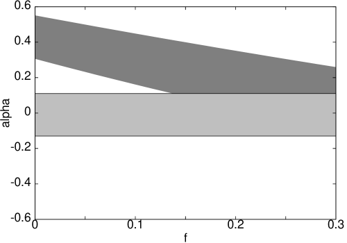
Figure 3: The parameter $\alpha$ as a function of the fraction of $J/\psi$ produced by decay of $\chi_{1,2}$. The dark band is the prediction for $f=f_{1}=f_{2}$. The lighter horizontal band is the 1-$\sigma$ range for $\alpha$ seen in $T=0$ experiments.

Consider now nucleus-nucleus collisions where the central rapidity region reaches a temperature sufficient to suppress $\chi$ but not $J/\psi$ [15], i. e., $f_{1}(T)\approx f_{2}(T)\approx 0$. The total $J/\psi$ cross section should decrease by about 50%. Simultaneously the angular distribution should change, with a new $\zeta=3/7$. As shown in Figure 3, the change should be easily visible.

Thermal effects on $\Upsilon$ have not been considered earlier, since this resonance is not expected to dissolve at the temperatures which the LHC may reach [15]. However, the $\chi_{b}$ states are expected to disappear at such temperatures [15]. Our earlier analysis would then lead us to believe that some reduction of the $\Upsilon$ cross section may occur, and the angular distribution may change to give $\alpha_{\Upsilon}=3/7$. Since the successive disappearance of different quarkonium states can be used for thermometry of the plasma, we believe it is important to look for this effect.

We present a list of experiments which might be used to constrain and test the applicability of NRQCD to inclusive quarkonium hadroproduction.

• More refined measurements of the cross sections for $\chi_{1}$ and $\chi_{2}$ production with proton and pion beams, at $\sqrt{S}\approx 40$ GeV, should test the scaling of the matrix elements and fix the ratio $R_{J/\psi}/R_{\chi}$. High-statistics experiments at $\sqrt{S}<25$ GeV designed to see the difference in $f_{1}/f_{2}$ for proton and pion would be welcome.

• Measurement of angular correlations in the decay $\chi\to\gamma e^{+}e^{-}$ would test the dipole dominance model of this decay, and hence the NRQCD explanation of the angular distribution. Hadroproduction experiments are not needed for this. In fact $e^{+}e^{-}$ machines, such as the LEP, would be preferable.

• Present day errors on $\alpha$ are large, and need to be reduced significantly. Simultaneous measurements of $f_{1}$, $f_{2}$ and $\alpha$ by one experiment can test NRQCD scaling rather accurately.

• The $\bar{b}b$ system remains almost completely unexplored. Due to the smallness of $v^{2}$ in this system, one would expect the phenomenology to be quite different from the $\bar{c}c$ system, and scaling arguments to work better. In view of the importance of $\Upsilon$ and $\chi_{b}$ for tests of NRQCD scaling, and possible applications to the thermometry of a quark-gluon plasma, a vigorous experimental effort in this field would pay large dividends.

The results can be summarized as follows— an NRQCD based argument yields $\alpha_{J/\psi}\approx 0$, provided the scaling formula of eq. (2.4) is used. The effective angular distribution (eq. 4.3) needs three parameters related to angular correlations in the decays $\chi_{J}\to\gamma J/\psi$. They need not be fine tuned to reproduce the observed angular distributions, although the assumption that the decays proceed through an electric dipole transition is supported. A crude estimate for the $\bar{b}b$ system gives $\alpha_{\Upsilon}\approx 0.25$–0.70. These findings may be applied to the $J/\psi$ suppression signal for the formation of a quark-gluon plasma— a suppression should be coupled with a large change in $\alpha$, since the feed-down processes disappear rapidly with increasing temperature. Suppression of $\chi_{b}$ should similarly influence the angular distribution of $\Upsilon$.

Appendix A Computing the coefficient functions

We take the momenta of the initial particles, $p_{1}$ and $p_{2}$, and the momentum of the pair, $P=p_{1}+p_{2}$ ($P^{2}=M^{2}$), to lie along the $z$-direction. We choose $p_{1}^{z}>0$ and take this to be the axis of quantization of angular momenta. The 4-momenta of $Q$ and $\bar{Q}$ ($p$ and $\bar{p}$ respectively, $p^{2}=\bar{p}^{2}=m^{2}$) are written as

$$p\;=\;{1\over 2}P+L_{j}q^{j}\qquad{\rm and}\qquad\bar{p}\;=\;{1\over 2}P-L_{j}q^{j}.$$ (A.1)

The space-like vector $q$ is defined in the rest frame of the pair, and $L^{\mu}_{j}$ boosts it to any frame. For $gg$ initial states we choose polarization vectors

$$\epsilon^{1}(\lambda)\;=\;{1\over\sqrt{2}}(0,-\lambda,-i,0)\qquad{\rm and}\qquad\epsilon^{2}(\lambda)\;=\;{1\over\sqrt{2}}(0,\lambda,-i,0).$$ (A.2)

Since the polarization vectors are orthogonal to both the initial momenta, this corresponds to a choice of planar gauge.

Euclidean 3-tensors are expressed as spherical tensors. As an example, a 3-vector $a_{i}$ is written as a spherical tensor of rank 1, with components

$$a_{\pm 1}\;=\;\mp{1\over\sqrt{2}}\left(a_{x}\pm ia_{y}\right),\quad a_{0}\;=\;a_{z}.$$ (A.3)

In this representation

$$\epsilon^{1}(\lambda)\cdot L_{m}\;=\;-\delta_{m,\lambda},$$ (A.4)

where $m$ is a helicity index. An useful identity is

$$a_{j}b_{j}\;=\;a_{0}b_{0}-(a_{+1}b_{-1}+a_{-1}b_{+1})\;=\;-\sqrt{3}[a,b]^{0}_{0},$$ (A.5)

We have introduced the notation $[a,b]^{J}_{M}$ to denote two vectors $a$ and $b$ coupled to total rank $J$ and helicity $M$. The coefficient of the terms $[a,b]^{0}_{0}$ can be obtained from the appropriate Clebsch-Gordan coefficients.

Since we work to lowest order in the QCD coupling, the perturbative projector is

$$\Pi(\bar{Q}Q)\;=\;|\bar{Q}Q\rangle\langle\bar{Q}Q|.$$ (A.6)

Its normalisation is completely fixed by the relativistic normalisation of states

$$\langle Q(p,\xi)\bar{Q}(\bar{p},\eta)|Q(p^{\prime},\xi^{\prime})\bar{Q}(\bar{p}^{\prime},\eta^{\prime})\rangle\;=\;4E_{p}E_{\bar{p}}(2\pi)^{6}\delta^{3}(p-p^{\prime})\delta^{3}(\bar{p}-\bar{p}^{\prime}),$$ (A.7)

where the spinor normalisations are $\xi^{\dagger}\xi=\eta^{\dagger}\eta=1$. Expanding $E_{p}=E_{\bar{p}}=\sqrt{m^{2}+q^{2}}$ in $q^{2}$ allows us to write any spinor bilinear in terms of transition operators built out of heavy quark fields.

The matrix element for the subprocess $\bar{q}q\to\bar{Q}Q$ has been treated to leading order in $v$ in [8]. The result, $\zeta_{\bar{q}q}=0$ for all quarkonium states, can be trivially generalized to all orders in $v$. The squared matrix element can be written in the form

$$|{\cal M}|^{2}\;=\;\left[k_{1}\cdot L_{i}k_{2}\cdot L_{j}+k_{2}\cdot L_{i}k_{1}\cdot L_{j}-k_{1}\cdot k_{2}L_{i}\cdot L_{j}\right]W^{ij},$$ (A.8)

where $W^{ij}$ represents the square of a heavy-quark spinor bilinear. In the kinematics appropriate for this problem, the prefactor to $W^{ij}$ becomes $(1-\delta_{i3}\delta_{j3})$. Transforming to spherical tensor components, this can be seen to give a vanishing longitudinal cross section.

The computations for the $gg$ process can easily become tedious. We introduce here a helicity technique based on a decomposition of the matrix element into gauge invariant amplitudes—

$${\cal M}\;=\;{1\over 6}g^{2}\delta_{ab}S+{1\over 2}g^{2}d_{abc}D^{c}+{i\over 2}g^{2}f_{abc}F^{c}.$$ (A.9)

These amplitudes have been enumerated earlier [13].

The invariant amplitudes are most compactly written in terms of two quantities $\cal A$ and $\cal S$. When the initial gluon helicities are $\lambda$ and $\lambda^{\prime}$, with the gauge choice given earlier, we get

$${\cal A}\;=\;{1\over 2}i\lambda\delta_{\lambda,\lambda^{\prime}}\quad{\rm and}\quad{\cal S}_{ij}a^{i}b^{j}\;=\;-\sqrt{3}\left[a,b\right]^{0}_{0}\delta_{\lambda,\lambda^{\prime}}+\sqrt{2}\left[a,b\right]^{2}_{2\lambda}\delta_{\lambda,-\lambda^{\prime}}$$ (A.10)

In order to identify all terms to order $v^{9}$ we need the colour amplitude $S$ to order $q^{5}$—

$$\begin{array}[]{rl}S&=\;-\left({\displaystyle 8im\over\displaystyle M}\right){\cal A}\,(\xi^{\dagger}\eta)+{\displaystyle 4\over\displaystyle M}{\cal S}_{jm}\,(q^{m}\xi^{\dagger}\sigma^{j}\eta)-\left({\displaystyle 32im\over\displaystyle M^{3}}\right){\cal A}\hat{z}_{m}\hat{z}_{n}\,(q^{m}q^{n}\xi^{\dagger}\eta)\\ &\qquad\quad+{\displaystyle 16\over\displaystyle M^{3}}\left[{\cal S}_{jm}\hat{z}_{n}\hat{z}_{p}-{\displaystyle M\over\displaystyle M+2m}\delta_{jm}{\cal S}_{np}\right]\,(q^{m}q^{n}q^{p}\xi^{\dagger}\sigma^{j}\eta)\\ &\qquad\qquad-\left({\displaystyle 128im\over\displaystyle M^{5}}\right){\cal A}\hat{z}_{m}\hat{z}_{n}\hat{z}_{p}\hat{z}_{r}\,(q^{m}q^{n}q^{p}q^{r}\xi^{\dagger}\eta)\\ &\quad\quad+{\displaystyle 64\over\displaystyle M^{5}}\left[{\cal S}_{jm}\hat{z}_{n}\hat{z}_{p}-{\displaystyle M\over\displaystyle M+2m}\delta_{jm}{\cal S}_{np}\right]\hat{z}_{r}\hat{z}_{s}\,(q^{m}q^{n}q^{p}q^{r}q^{s}\xi^{\dagger}\sigma^{j}\eta).\end{array}$$ (A.11)

The amplitude $D$ differs only through having colour octet matrix elements in place of the colour singlet ones shown above. For the colour amplitude $F$ we need the expansion

$$F^{c}\;=\;-\left({\displaystyle 16im\over\displaystyle M^{2}}\right){\cal A}\hat{z}_{m}\,(q^{m}\xi^{\dagger}T^{c}\eta)+{\displaystyle 8\over\displaystyle M^{2}}{\cal S}_{jm}\hat{z}_{n}\,(q^{m}q^{n}\xi^{\dagger}\sigma^{j}T^{c}\eta).$$ (A.12)

In all three colour amplitudes, the terms in ${\cal A}$ are spin singlet and those in ${\cal S}$ are spin triplet.

The structure is very simple. Conservation of angular momentum shows that the $J_{z}=0$ terms are obtained when $\lambda=\lambda^{\prime}$. With eq. (A.10) recoupling of all spherical tensors into terms of well-defined $L$, $S$ and $J$ can now be performed at the amplitude level. This also simplifies the computations presented in [13]. The full procedure, from this recoupling to the computation of the coefficient functions can be reduced to a Mathematica program.

References

- [1] M. E. Rose, “Elementary Theory of Angular Momentum”, John Wiley and Sons, New York, 1957.
- [2] A. Gribushin et al., Phys. Rev., D 53 (1996) 4723.
-
[3]
J. G. Heinrich et al., Phys. Rev. D 44 (1991) 1909;
C. Akerlof et al., Phys. Rev. D 48 (1993) 5064;
T. Alexopoulos et al., Phys. Rev. D 55 (1997) 3927. - [4] P. Cho and M. Wise, Phys. Lett., B 346 (1995) 129.
-
[5]
W.E. Caswell and G.P. Lepage, Phys. Lett., B 167 (1986) 437;
G. T. Bodwin, E. Braaten and G. P. Lepage, Phys. Rev., D 51 (1995) 1125; [Erratum ibid., D 55 (1997) 5853]. - [6] M. Beneke and I. Rothstein, Phys. Lett., B 372 (1996) 137; [Erratum: ibid. B 389 (1996) 789].
- [7] M. Beneke and I. Rothstein, Phys. Rev., D 54 (1996) 2005; [Erratum: ibid. D 54 (1996) 7082].
- [8] E. Braaten and Y. Chen, Phys. Rev., D 54 (1996) 3216.
- [9] M. Beneke, preprint hep-ph/9703429, to appear in the Proceedings of the XXIVth SLAC Summer Institute on Particle Physics, August 1996.
- [10] S. Baek, P. Ko, J. Lee and H. S. Song, Phys. Rev., D 55 (1997) 6839.
- [11] S. Gupta and K. Sridhar, Phys. Rev., D 54 (1996) 5545.
- [12] S. Gupta and K. Sridhar, Phys. Rev., D 55 (1997) 2650.
-
[13]
S. Gupta and P. Mathews, Phys. Rev., D 56 (1997) 3019;
S. Gupta and P. Mathews, Phys. Rev., D 56 (1997) 7341. - [14] T. Matsui and H. Satz, Phys. Lett., B 178 (1986) 416.
- [15] F. Karsch and H. Satz, Z. Phys., C 51 (1991) 209.
-
[16]
E. Braaten, M. A. Doncheski, S. Fleming and M. Mangano,
Phys. Lett., B 333 (1994) 548;
D. P. Roy and K. Sridhar, Phys. Lett., B 339 (1994) 141;
M. Cacciari and M. Greco, Phys. Rev. Lett., 73 (1994) 1586. - [17] A. Petrelli, M. Cacciari, M. Greco, F. Maltoni and M. L. Mangano, preprint hep-ph/9707223.
- [18] M. Beneke and M. Kramer, Phys. Rev., D 55 (1997) 5269.
-
[19]
M. Gluck, E. Reya and A. Vogt, Z. Phys., C 67 (1995) 433;
M. Gluck, E. Reya and A. Vogt, Z. Phys., C 53 (1992) 651. -
[20]
D. A. Bauer, et al., Phys. Rev. Lett., 54 (1985) 753;
L. Antoniazzi et al., Phys. Rev., D 49 (1994) 543. - [21] K. Hagan et al. (E 771), to appear in the Proceedings of the Quarkonium Physics Workshop, University of Illinois, Chicago, June 1996; measurements quoted in [9].
-
[22]
M. Vänttinen, P. Hoyer, S. J. Brodsky and W.-K. Tang,
Phys. Rev., D 51 (1995) 3332;
W.-K. Tang and M. Vänttinen, Phys. Rev., D 54 (1996) 4349. - [23] V. Koreshev et al., Phys. Rev. Lett., 77 (1996) 4294.