1. Recently there has been renewed interest in off-diagonal parton distributions, i.e. in correlation functions of quark or gluon fields between different nucleon states, which have been introduced some time ago [1]. They appear for instance in the description of exclusive photon or meson production in $\gamma^{\ast}p$ collisions at large photon virtuality $Q^{2}$ and small squared momentum transfer $t$ of the proton [2–5], showing up as the long distance nonperturbative quantities when one factorises the transition amplitude into short and long distance subprocesses. In meson electroproduction there is yet another nonperturbative ingredient, namely the meson distribution amplitude which describes the transition from the valence quarks to the final vector meson. The corresponding diagrams are shown in Fig. 1.

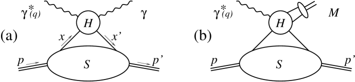
Figure 1: Diagrams for $\gamma^{\ast}p\to Ap$ at large $Q^{2}$ and small $t$, where $A$ is $(a)$ a real photon or $(b)$ a meson $M$. They consist of an off-diagonal parton distribution, a hard scattering part, and a meson distribution amplitude in case $(b)$. The partons connecting $S$ and $H$ have momenta $k$ and $k^{\prime}$ with plus components $k^{+}=xp^{+}$ and $k^{\prime+}=x^{\prime}p^{+}$.

The relevance of off-diagonal parton distributions is not restricted to these processes. In particular the asymmetric gluon distribution has been considered in several $\gamma^{\ast}p$ processes at small Bjorken $x$, such as diffractive production of dijets and of heavy quarks [6]. For exclusive $J/\psi$ production one may relax the requirement of large $Q^{2}$ because of the large meson mass [7], as well as for the exclusive production of a $Z$ boson [8].

2. Let us first have a closer look at the kinematics of the reactions we have in mind. We denote particle momenta according to

$$\gamma^{\ast}(q)+p(p)\to A(q^{\prime})+p(p^{\prime})\hskip 6.0pt,\hskip 6.0pt$$ (1)

where $A$ is a meson, real photon or heavy gauge boson, or a quark-antiquark pair in a diffractive process. One might also have a virtual $Z$ or $W$ instead of the $\gamma^{\ast}$ and/or $A$ may be charged, replacing the initial or final state proton by a neutron as necessary. We will use the momentum transfer $\Delta=p-p^{\prime}$ from the proton, and the invariants $t=\Delta^{2}$, $W^{2}=(p+q)^{2}$, $Q^{2}=-q^{2}$, $m_{A}^{2}=q^{\prime 2}$, $m_{p}^{2}=p^{2}$.

We now consider those reference frames where the incoming photon and proton are collinear. Picking out any one of them we choose the $z$ axis along the proton momentum $p$ and introduce two lightlike vectors

$$v=\frac{1}{\sqrt{2}}\,(1,0,0,1)\hskip 6.0pt,\hskip 6.0pt\hskip 20.00003ptv^{\prime}=\frac{1}{\sqrt{2}}\,(1,0,0,-1)\hskip 6.0pt,\hskip 6.0pt$$ (2)

which respectively set a plus and minus direction. We can write

$$p^{\mu}=p^{+}\,v^{\mu}+\frac{m_{p}^{2}}{2p^{+}}\,v^{\prime\mu}\hskip 6.0pt,\hskip 6.0pt\hskip 20.00003pt\Delta^{\mu}=\xi p^{+}\,v^{\mu}-\frac{m_{p}^{2}\xi+{\bf\Delta}_{T}^{2}}{2p^{+}(1-\xi)}\,v^{\prime\mu}+\Delta_{T}^{\mu}$$ (3)

and

$$t=-\frac{m_{p}^{2}\xi^{2}+{\bf\Delta}_{T}^{2}}{1-\xi}\hskip 6.0pt,\hskip 6.0pt$$ (4)

having defined the variable $\xi=\Delta^{+}/p^{+}$, whose exact expression in terms of the invariants listed above we will not need here. We further have

$$q^{\mu}=-x_{N}p^{+}\,v^{\mu}+\frac{Q^{2}}{2p^{+}x_{N}}\,v^{\prime\mu}\hskip 6.0pt,\hskip 6.0pt$$ (5)

where

$$x_{N}=\frac{2x_{B}}{1+\sqrt{1+4x_{B}^{2}m_{p}^{2}/Q^{2}}}$$ (6)

is Nachtmann’s and $x_{B}=Q^{2}/(2p\cdot q)$ Bjorken’s scaling variable. From the positivity of particle energies in the final state one obtains

$$x_{N}\leq\xi<1\hskip 6.0pt.\hskip 6.0pt$$ (7)

To ensure that the blob $H$ in Fig. 1 corresponds to a hard scattering we require that at least one of $Q^{2}$ and $m_{A}^{2}$ be large compared with a GeV². For the blob $S$ to be a soft, long distance quantity one will need that the transverse bend $|{\bf\Delta}_{T}|$ is of the order of a hadronic scale.

The threshold region is special in its dynamics: apart from the formation of resonances one can expect strong rescattering effects between $A$ and the outgoing proton which may destroy factorisation. One will ask for $W-m_{A}-m_{p}\gg 1\mbox{\ GeV}$ to exclude this region. It can be shown that this is equivalent to limiting the range of $\xi$ to $1-\xi\gg(m_{p}\,W)/(W^{2}+Q^{2})$, which according to (4) also puts an upper limit on $-t$. Up to corrections of order $m_{p}^{2}/(W^{2}-m_{A}^{2})$ and ${\bf\Delta}_{T}^{2}/(W^{2}-m_{A}^{2})$ one then has

$$\xi=\frac{Q^{2}+m_{A}^{2}}{2p\cdot q}\hskip 6.0pt.\hskip 6.0pt$$ (8)

Under these conditions one can find a frame, e.g. the $\gamma^{\ast}p$ c.m., where the initial proton is moving fast and collides head on with the photon, $p^{+}\gg m_{p}$, and where the scattered proton is fast as well, $p^{\prime+}\gg m_{p}$. Such a frame is natural for a partonic interpretation of our process.

3. The nonperturbative transition from the proton to the parton level (see Fig. 1) is described by a two-point function of the form

$$M=\frac{1}{2\pi}\int dz^{-}\,e^{ixp^{+}z^{-}}\left.\langle p^{\prime},\sigma^{\prime}\,|\,T\,\bar{\psi}(0)\gamma^{+}\psi(z)\,|\,p,\sigma\rangle\right|_{z=z^{-}\,v^{\prime}}\hskip 6.0pt.\hskip 6.0pt$$ (9)

This representation holds in the $A^{+}=0$ gauge, where $A^{\mu}$ is the gluon potential; for other gauges one has to insert the standard path ordered exponential between the two quark fields. Instead of $\gamma^{+}$ in (9) there can be other Dirac matrices, which in order to give a leading twist contribution must transform like $\gamma^{+}$ under a longitudinal boost. Which matrices are relevant depends on the process considered; in virtual Compton scattering, $\gamma^{\ast}p\to\gamma p$, one needs for instance $\gamma^{+}$ and $\gamma^{+}\gamma_{5}$. There are also contributions from two-point functions where gluon field strengths replace the quark fields in (9).

We notice that these quark and gluon two-point functions depend on the spins $\sigma$ and $\sigma^{\prime}$ of the initial and final state proton. This spin structure can be made explicit by writing (9) as a sum of Dirac bilinears for the proton multiplied by scalar functions $F_{i}(x,\xi,t)$. It is these functions that are called off-diagonal parton distributions; we will not need their explicit definitions here. For ease of writing we will not explicitly display the labels $\sigma$ and $\sigma^{\prime}$ henceforth.

The usual parton distributions that occur in inclusive deep inelastic scattering involve diagonal matrix elements of quark fields or gluon field strengths, i.e. they correspond to the limit $p^{\prime}=p$ and $\sigma^{\prime}=\sigma$ in (9). The variables $\xi=\Delta^{+}/p^{+}$ and $t=\Delta^{2}$ are then zero since $\Delta=0$. The diagrams that describe inclusive deep inelastic scattering are obtained by cutting the ones of Fig. 1 $(a)$ with the real photon replaced by a virtual one.

At this point we note that because the proton states in (9) are different the off-diagonal distributions do not have any probabilistic interpretation, contrary to the usual parton distributions. In particular one cannot expect the $F_{i}$ to have a definite sign as ordinary quark or gluon densities, which are nonnegative for $0<x<1$.

4. When calculating the transition amplitude from the diagrams in Fig. 1 the soft blob describing the proton-parton coupling translates into the Fourier transformed matrix element of a time ordered product of parton operators. We will show that one can actually drop the time ordering and instead use ordinary products.

The same problem has long ago been considered by Jaffe [9] for the parton distributions in deep inelastic scattering. For the deep inelastic cross section one needs the absorptive part of the forward $\gamma^{\ast}p\to\gamma^{\ast}p$ amplitude, cutting the diagrams including the soft blob, and naturally obtains ordinary products instead of time ordered ones. It was however shown in [9] that the ordinary product already appears in the full amplitude, not only its absorptive part. The same result also follows from early work by Landshoff and Polkinghorne [10], without being explicitly stated there, and we will apply their method to the non-diagonal case here.

The fact that one can omit time ordering in the parton distributions has important consequences for their support properties in the scaling variable $x$, which in turn are crucial for their interpretation in terms of partons [9, 11]. In the off-diagonal case it is also needed if one wants to derive a dispersion relation for the scattering amplitude [4]. Furthermore it allows one to constrain the two-point function (9) using time reversal invariance: together with parity invariance one finds that the phases of the scalar parton distributions $F_{i}(x,\xi,t)$ are a matter of convention, so that they can be defined as real valued.

As a by-product of the demonstration we will obtain the support properties for $F_{i}$ in $x$ and identify different regions in $x$ according to whether the partons are in the initial or final state of the hard scattering $H$. This generalises the results obtained in [9] concerning the support and partonic interpretation of the usual densities to the case of off-diagonal distributions.

5. Let us first consider the quark two-point function $M$ of (9). Our arguments will be unchanged if $\gamma^{+}$ is replaced by another suitable Dirac matrix. We rewrite

$$M=\frac{1}{(2\pi)^{4}}\int d^{2}{\bf k}_{T}\,dk^{-}\,\left.{\cal A}\right|_{k^{+}=xp^{+}}$$ (10)

where

$${\cal A}=\int d^{4}z\,e^{ik\cdot z}\langle p^{\prime}\,|\,T\,\bar{\psi}(0)\gamma^{+}\psi(z)\,|\,p\rangle$$ (11)

is an amplitude describing the scattering of an off-shell antiquark with momentum $-k$ on an on-shell proton with momentum $p$,

$$p(p)+\bar{q}(-k)\to p(p^{\prime})+\bar{q}(-k^{\prime})\hskip 6.0pt.\hskip 6.0pt$$ (12)

Note that this amplitude is not truncated in the parton legs. The plus components $k^{+}=xp^{+}$ and $k^{\prime+}=x^{\prime}p^{+}$ with $x^{\prime}=x-\xi$ are kept fixed in the following.

The kinematical invariants $\cal A$ depends on are the virtualities $k^{2}$ and $k^{\prime 2}$ and the Mandelstam variables $s=(-k+p)^{2}$, $u=(k+p^{\prime})^{2}$ and $t$, the latter being fixed by the kinematics of the reaction (1). Following [10] we assume that the analytical properties of $\cal A$ are the usual ones known from the study of Feynman diagrams, i.e. that it has cuts for nonnegative $\mbox{Re}\,s$, $\mbox{Re}\,u$ and singularities for nonnegative $\mbox{Re}\,k^{2}$ and $\mbox{Re}\,k^{\prime 2}$. In the standard conventions, these singularities are slightly below the real axis of these variables.

We can carry out the integration over $k^{-}$ in (10) taking into account the singularity structure of $\cal A$. To see where the singularities are located in the complex $k^{-}$ plane we in turn express $k^{-}$ through one of the invariants $s$, $k^{\prime 2}$, $k^{2}$, $u$, supplemented by $x$, ${\bf k}_{T}$ and the variables in (3) which are all kept fixed during the $k^{-}$ integration:

$$k^{-} = {s+{\bf k}_{T}^{2}\over 2p^{+}(x-1)}+p^{-}\hskip 6.0pt,\hskip 6.0pt$$ (13)

$$k^{-} = {k^{\prime 2}+({\bf k}_{T}-{\bf\Delta}_{T})^{2}\over 2p^{+}(x-\xi)}+\Delta^{-}\hskip 6.0pt,\hskip 6.0pt$$

$$k^{-} = {k^{2}+{\bf k}_{T}^{2}\over 2p^{+}x}\hskip 6.0pt,\hskip 6.0pt$$

$$k^{-} = {u+({\bf k}_{T}-{\bf\Delta}_{T})^{2}\over 2p^{+}(x+1-\xi)}-p^{-}+\Delta^{-}\hskip 6.0pt.\hskip 6.0pt$$

There is a sequence of sign changes of the above denominators as $x$ varies from $-\infty$ to $+\infty$. Using $0\leq\xi<1$ we see that they occur at $x=\xi-1$, $0$, $\xi$ and $1$. These signs determine whether the singularities of $\cal A$ are located above or below the real axis in the $k^{-}$ plane.

For $x\leq\xi-1$ and $x\geq 1$ all singularities lie on the same side of the real $k^{-}$ axis and we can close the contour in the other half plane without encircling any singularity. The $k^{-}$ integral vanishes and we deduce that

$M$ is only nonzero for $\xi-1<x<1$.

To be able to close the integration contour in the $k^{-}$ plane we have made the dynamical assumption that $\cal A$ vanishes sufficiently fast as $k^{-}$ tends to infinity in the complex plane while $k^{+}$ and ${\bf k}_{T}$ are fixed, a limit in which the parton virtualities $k^{2}$ and $k^{\prime 2}$ become infinite. Note that we have not yet integrated over ${\bf k}_{T}\,$: as remarked in [9] the integration of $\cal A$ over ${\bf k}_{T}$ and $k^{-}$ leads to ultraviolet divergences, but this does not contradict our assumption that the integral over $k^{-}$ alone is sufficiently well behaved. The full integration over ${\bf k}_{T}$ and $k^{-}$ can only be done in a suitably regularised theory; it is known from the usual parton distributions that the corresponding renormalisation of the integral (10) is intimately related with their logarithmic evolution in QCD.

Let us now discuss in turn the regions of $x$ in the interval $\xi-1<x<1$. Details of the argument are given in the Appendix.

• In the region $\xi\leq x<1$, the $s$ singularities are in the upper half plane of $k^{-}$ whereas all other singularities are in the lower half plane. Wrapping the $k^{-}$ contour around the $s$ cuts gives

  $$\int_{-\infty}^{+\infty}dk^{-}\,{\cal A}=\int dk^{-}\,{\rm disc}_{s}{\cal A}\hskip 6.0pt,\hskip 6.0pt$$ (14)

  where ${\rm disc}_{s}{\cal A}$ is the discontinuity of $\cal A$ across the cuts in $s$. We use now the standard reasoning on the matrix element

  $$\widehat{M} = \frac{1}{2\pi}\int dz^{-}\,e^{ixp^{+}z^{-}}\left.\langle p^{\prime}\,|\,\bar{\psi}(0)\gamma^{+}\psi(z)\,|\,p\rangle\right|_{z=z^{-}\,v^{\prime}}$$ (15)

  $$= \frac{1}{(2\pi)^{4}}\int d^{2}{\bf k}_{T}\,dk^{-}\left.\int d^{4}z\,e^{ik\cdot z}\langle p^{\prime}\,|\,\bar{\psi}(0)\gamma^{+}\psi(z)\,|\,p\rangle\right|_{k^{+}=xp^{+}}$$

  which does not involve time ordering, inserting a complete set of intermediate states between $\bar{\psi}(0)\gamma^{+}$ and $\psi(z)$ as illustrated in Fig. 2 $(a)$. In line with our assumptions on its analyticity properties we assume that one can apply the cutting rules to ${\cal A}$ as one would for Feynman diagrams, and obtain

  $$M=\frac{1}{(2\pi)^{4}}\int d^{2}{\bf k}_{T}\,dk^{-}\,{\rm disc}_{s}{\cal A}=\widehat{M}\hskip 6.0pt.\hskip 6.0pt$$ (16)

  In this region of $x$ we can interpret $M$ as the amplitude for the proton emitting a quark with light cone fraction $x$ and reabsorbing it with light cone fraction $x^{\prime}$.

• In the region $\xi-1<x\leq 0$, the $u$ singularities are alone below the real $k^{-}$ axis and we can write

  $$\int_{-\infty}^{+\infty}dk^{-}\,{\cal A}=\int dk^{-}{\rm disc}_{u}{\cal A}\hskip 6.0pt.\hskip 6.0pt$$ (17)

  We now consider the scattering process

  $$p(p)+q(k^{\prime})\to p(p^{\prime})+q(k)\hskip 6.0pt,\hskip 6.0pt$$ (18)

  whose amplitude is given by $-{\cal A}$, where the minus sign comes from interchanging the quark and antiquark field under the time ordering in (11). Defining

  $$\widehat{M}^{\prime}=-\frac{1}{2\pi}\int dz^{-}\,e^{ixp^{+}z^{-}}\left.\langle p^{\prime}\,|\,\psi(z)\;\bar{\psi}(0)\gamma^{+}\,|\,p\rangle\right|_{z=z^{-}\,v^{\prime}}\hskip 6.0pt,\hskip 6.0pt$$ (19)

  and repeating our above argument we find

  $$M=\frac{1}{(2\pi)^{4}}\int d^{2}{\bf k}_{T}\,dk^{-}\,{\rm disc}_{u}{\cal A}=\widehat{M}^{\prime}\hskip 6.0pt.\hskip 6.0pt$$ (20)

  In the present region of $x$ we can interpret $M$ as corresponding to the emission by the proton of an antiquark with momentum fraction $-x^{\prime}$ and its reabsorption with momentum fraction $-x$.

• The intermediate region, $0<x<\xi$, is more involved since the singularities in $s$ and $k^{\prime 2}$ lie in the upper half plane of $k^{-}$ while those in $u$ and $k^{2}$ lie in the lower half plane. We notice that in this case $x>0$ and $x^{\prime}<0$, i.e. in this situation one has a quark and an antiquark flowing out of the initial state. This configuration is specific of the off-diagonal matrix element, and in [3, 5] its reminiscence of the quark-antiquark distribution amplitude of a meson has been emphasised.

  If we choose to close the $k^{-}$ contour in the upper half plane we can write the integral over $k^{-}$ of $\cal A$ as a sum of terms due to the singularities in $s$ and in $k^{\prime 2}$,

  $$\int_{-\infty}^{+\infty}dk^{-}\,{\cal A}=\int dk^{-}\,\Big{(}{\rm disc}_{s}{\cal A}+\{\mbox{terms from $k^{\prime 2}$ singularities}\}\Big{)}\hskip 6.0pt,\hskip 6.0pt$$ (21)

  where the singularities in $k^{\prime 2}$ are cuts and a mass pole, cf. the Appendix. Having chosen this representation we consider again $\widehat{M}$ and the scattering (12), but now when we insert a complete set of states, the kinematics allow intermediate states that already contain the outgoing proton, $|X\rangle=|p^{\prime}X^{\prime}\rangle$. For those states there are diagrams which are disconnected at the right-hand side of the cut, cf. Fig. 2 $(b)$, and correspond to a cut in the variable $k^{\prime 2}$. They give just the extra terms in (21) and the cutting rules now allow us to write

  $$M=\frac{1}{(2\pi)^{4}}\int d^{2}{\bf k}_{T}\,dk^{-}\Big{(}{\rm disc}_{s}{\cal A}+\{\mbox{terms from $k^{\prime 2}$ singularities}\}\Big{)}=\widehat{M}\hskip 6.0pt.\hskip 6.0pt$$ (22)

In all three regions of $x$ there are of course two ways to pick up singularities in the $k^{-}$ plane: those in the upper half will lead to $\widehat{M}$ and those in the lower half to $\widehat{M}^{\prime}$. The situation is summarised in Fig. 2. In regions A and B we have a simple physical interpretation if we pick up the $s$ and $u$ cut, respectively, as was already discussed for diagonal densities in [9], whereas in region C the choices $s$, $k^{\prime 2}$ and $u$, $k^{2}$ appear as symmetric to each other.

For all values of $x$ we then have

$$\rule[-8.61108pt]{0.0pt}{25.83325pt}M=\widehat{M}=\widehat{M}^{\prime}\hskip 6.0pt,\hskip 6.0pt$$ (23)

i.e. we can drop the time ordering in $M$ and write quark and antiquark field in any order. Our argument shows that the origin of this is the integration over $k^{-}$, which corresponds to fields being evaluated at the same light cone time ($z^{+}=0$). We could in fact apply it without integrating over ${\bf k}_{T}$ at all to obtain the analogue of (23) for ${\bf k}_{T}$ unintegrated parton densities.

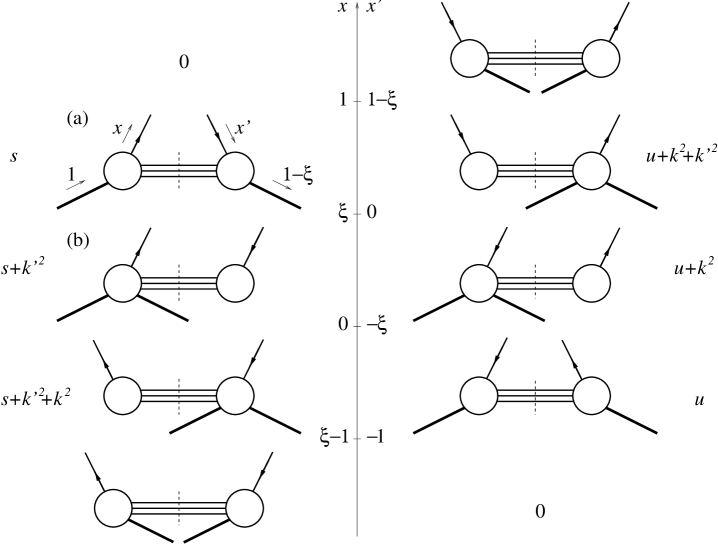
Figure 2: The two alternatives to pick up singularities in the $k^{-}$ plane, depending on the region of $x$. To the left (right) are the singularities above (below) the real $k^{-}$ axis. The diagrams show the new cut as one changes from one region of $x$ to the next, going from top to bottom on the left and from bottom to top on the right. We also give an axis in $x^{\prime}$ to display the symmetry between the two partons.

6. Our preceding discussion can be applied to off-diagonal gluon distributions in an analogous way by considering the amplitude for the scattering of an off-shell gluon on the proton. Note that one then deals with products of gluon potentials $A^{\mu}$, while the gluon distributions are defined in terms of gluon field strengths $G^{\mu\nu}$. The passage from one to the other is however simple in the $A^{+}=0$ gauge, since the leading twist distributions only involve $G^{+\nu}$ which in this gauge reduces to $\partial^{+}A^{\nu}$. For a further discussion we refer to [5].

In the case of gluons there is no minus sign when one interchanges the order of the fields in the amplitude (11) as there was in point B. above, and correspondingly the analogue of $\widehat{M}^{\prime}$ is defined without a minus sign.

We also remark that there are symmetry relations for the gluon distributions under the change $x\to-x^{\prime}=\xi-x$ in their first argument, so that it is enough to know them for $x\geq\xi/2$. In fact the diagrams in Fig. 1 with gluon lines between $S$ and $H$ remain the same if one interchanges the light cone fractions $x$ and $-x^{\prime}$, since $H$ denotes a sum of several Feynman graphs.

7. As mentioned in the beginning, the diagrams of Fig. 1 $(b)$ for exclusive meson production contain not only off-diagonal parton distributions as nonperturbative input, but also the meson distribution amplitude, which is expressed in terms of a matrix element between the vacuum and the meson state $|M\rangle$. It is easy to show along the lines of argument developed so far that the time ordering of quark operators in the distribution amplitude can be omitted, just as in parton distributions, as we will briefly outline.

The distribution amplitude is defined in terms of a two-point function

$$\frac{1}{2\pi}\int dz^{+}\,e^{-iyq^{\prime-}z^{+}}\left.\langle M\,|\,T\,\bar{\psi}(z)\gamma^{-}\psi(0)\,|\,0\rangle\right|_{z=z^{+}\,v}$$ (24)

or a corresponding one with a different Dirac matrix; in order to suppress the path ordered exponential between the quark fields one now needs the $A^{-}=0$ gauge. In analogy to (10) this two-point function can be rewritten as an integral over ${\bf l}_{T}$ and $l^{+}$ at fixed $l^{-}=yq^{\prime-}$ of the amplitude for the transition

$$q(l)+\bar{q}(l^{\prime})\to M(q^{\prime})$$ (25)

from the valence quarks to the meson. This amplitude depends on the invariants $l^{2}$ and $l^{\prime 2}$. Writing

$$l^{+} = \frac{l^{2}+{\bf l}_{T}^{2}}{2q^{\prime-}y}\hskip 6.0pt,\hskip 6.0pt$$

$$l^{+} = \frac{l^{\prime 2}+({\bf l}_{T}-{\bf\Delta}_{T})^{2}}{2q^{\prime-}(y-1)}+q^{\prime+}$$ (26)

and closing the contour of the $l^{+}$ integration in the complex plane one immediately obtains that the distribution amplitude vanishes outside the region $0<y<1$. There one can express it in terms of singularities in either $l^{\prime 2}$ or $l^{2}$, obtaining matrix elements of $\bar{\psi}(z)\gamma^{-}\psi(0)$ or $-\psi(0)\,\bar{\psi}(z)\gamma^{-}$, respectively. The two possibilities are shown in Fig. 3.

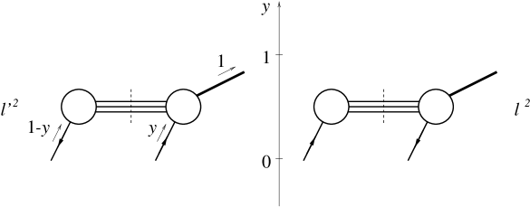
Figure 3: The two possibilities to pick up singularities in the $l^{+}$ plane for a meson distribution amplitude in the region $0<y<1$.

Comparing with the present situation we see again the hybrid nature of off-diagonal parton distributions in the region $0<x<\xi$ : the cuts in $s$ or $u$ are as in ordinary, diagonal parton distributions, whereas the singularities in the parton virtualities $l^{2}$ or $l^{\prime 2}$ are reminiscent of distribution amplitudes.

8. The fact that parton distributions and meson distribution amplitudes can be expressed in terms of cut amplitudes is important if one wants to show that the $s$-channel discontinuities of the $\gamma^{\ast}p$ amplitudes shown in Fig. 1 are obtained from appropriate cuts of the hard blob $H$, the soft quantities being “already cut”. Already of interest in the case of inclusive deep inelastic scattering this is essential for processes involving off-diagonal parton distributions, for instance when establishing a dispersion relation [4]. We shall not go into details here but wish to make some observations in connection with the results we have obtained so far.

There are different ways to cut the diagrams of Fig. 1 in the overall $s$-channel, i.e. in the variable $(p+q)^{2}$. If the hard blob $H$ is cut in $(q+k)^{2}$, which requires $x_{N}\leq x\leq 1$ to ensure positive energy across the cut, one can cut the soft blob $S$ in $s=(p-k)^{2}$; if $x\leq\xi$ one can also cut $S$ in $k^{\prime 2}$ or cut the parton line $k^{\prime}$ itself in the diagrams. The two-point function $M$ can be written in terms of just these cuts. As discussed in the appendix it includes in particular the term that comes from cutting the parton line $k^{\prime}$ and leads to a mass pole in the amplitude $\cal A$ of (11); hence this mass pole does not appear as an extra term in the expression of the discontinuity of the $\gamma^{\ast}p$ amplitude.

$H$ can also be cut in $(q-k^{\prime})^{2}$, then one must have $\xi-1\leq x\leq\xi-x_{N}$. This comes with cuts of $S$ in $u=(p+k^{\prime})^{2}$, and if $x\geq 0$ also with cuts in $k^{2}$ as well as the pole from cutting the parton line $k$. In this situation one will use the representation of $M$ in terms of singularities in $u$ and $k^{2}$. It is interesting to note that if there is a region $x_{N}\leq x\leq\xi-x_{N}$, e.g. in photoproduction of a heavy meson or a $Z$, one can have cuts of $H$ in both $(q+k)^{2}$ and $(q-k^{\prime})^{2}$ at the same value of $x$ and needs both representations of $M$ at the same time.

In the case of meson production (Fig. 1 $(b)$) one can also cut through the blob representing the meson distribution function, with one valence quark at either side of the cut, or one can cut through one of the valence quark lines. In this case one will use that the meson distribution amplitude can be written in terms of singularities in one of the quark virtualities $l^{2}$ and $l^{\prime 2}$ as discussed in sec. 7.

Acknowledgments
We gratefully acknowledge discussions with Jochen Bartels, Martin Beneke, John Collins, Peter Landshoff, Piet Mulders, Otto Nachtmann and Bernard Pire. Special thanks are due to O. Nachtmann for reading the manuscript. M. D. would like to thank the NIKHEF Theory Group for its hospitality.

T. G. was carrying out his work as part of a training Project of the European Community under Contract No. ERBFMBI–CT95–0411. This work has been partially funded through the European TMR Contract No. FMRX–CT96–0008: Hadronic Physics with High Energy Electromagnetic Probes. CPT is Unité Propre du CNRS and SUBATECH is Unité Mixte de l’Université de Nantes, de l’Ecole des Mines de Nantes et du CNRS.

Appendix
In this appendix we study in some detail the identity of the matrix elements $M$ and $\widehat{M}$ introduced respectively in (10) and (15). As we already mentioned the ${\bf k}_{T}$ integration has no relevance in the derivation so that we perform our reasoning on the corresponding ${\bf k}_{T}$ unintegrated quantity. We focus on the most complicated region $0<x<\xi$ where as discussed in point C. of sec. 5 the integration over $k^{-}$ inevitably picks up singularities in more than one invariant and where the cutting rules have to be applied with some care. In order to deal with complete but readable expressions we ignore here complexities due to the spin of both partons and hadrons and introduce

$${\cal M} = \int_{-\infty}^{+\infty}dk^{-}\int\!d^{4}z\,e^{ik\cdot z}\,\langle p^{\prime}|T\phi^{\dagger}(0)\phi(z)|p\rangle\hskip 6.0pt,\hskip 6.0pt$$ (27)

$$\widehat{{\cal M}} = \int_{-\infty}^{+\infty}dk^{-}\int\!d^{4}z\,e^{ik\cdot z}\,\langle p^{\prime}|\phi^{\dagger}(0)\phi(z)|p\rangle\hskip 6.0pt,\hskip 6.0pt$$

where $\phi$ is a charged scalar “quark” field and $|p\rangle$ a scalar “proton” state.

In the framework we are using we invoke perturbation theory for the purpose of analytic properties and of applying the cutting rules. To be consistent we must treat quarks as free particles with a mass $m_{q}$. The scalar analogue of the amplitude $\cal A$ in (11) then has cuts and a mass pole in each of $k^{2}$ and $k^{\prime 2}$. To apply the cutting rules we will isolate the poles from the rest of the singularity structure, and also keep track of possible disconnected terms of the matrix elements that appear in our argument. To this end we use the framework of the reduction formula [13] (cf. also [14]) and introduce an interpolating field $\mathit{\Phi}$ for the proton. For $p\neq p^{\prime}$ the matrix element $\langle p^{\prime}|T\phi^{\dagger}(0)\phi(z)|p\rangle$ does not have a disconnected part, and in the case of diagonal parton densities one explicitly only takes its connected part. One thus has

$$\int\!d^{4}z\,e^{ik\cdot z}\,\langle p^{\prime}|T\phi^{\dagger}(0)\phi(z)|p\rangle={i\sqrt{Z_{q}}\over k^{\prime 2}-m_{q}^{2}+i\varepsilon}\,{i\sqrt{Z_{q}}\over k^{2}-m_{q}^{2}+i\varepsilon}\,i\tilde{G}(p\bar{q}\to p^{\prime}\bar{q}^{\prime})$$ (28)

with

$$(2\pi)^{4}\delta^{(4)}(p-k-p^{\prime}+k^{\prime})\cdot i\tilde{G}=\frac{1}{Z_{q}}\,\frac{1}{Z_{p}}\,\int d^{4}z\,d^{4}z^{\prime}\,d^{4}y\,d^{4}y^{\prime}\,e^{ik\cdot z-ik^{\prime}\cdot z^{\prime}-ip\cdot y+ip^{\prime}\cdot y^{\prime}}\cdot$$ (29)

$$(\Box_{z^{\prime}}+m_{q}^{2})\,(\Box_{z}+m_{q}^{2})\,(\Box_{y^{\prime}}+m_{p}^{2})\,(\Box_{y}+m_{p}^{2})\cdot\langle 0|T\phi^{\dagger}(z^{\prime})\phi(z)\mathit{\Phi}(y^{\prime})\mathit{\Phi}^{\dagger}(y)|0\rangle\hskip 6.0pt,\hskip 6.0pt$$

where $Z_{q}$ and $Z_{p}$ are the wave function normalisation constants of the quark and the proton, and where four-momenta are labelled as in (12). In the limit where both parton legs go on shell $\tilde{G}$ is a $\cal T$-matrix element: depending on the signs of $k^{0}$ and $k^{\prime 0}$ the partons are in the initial or final state. We emphasise that only the parton mass poles in $k^{2}$ or $k^{\prime 2}$ have been isolated from $\tilde{G}$ which thus still contains the branch cuts in these variables, unlike truncated Green functions where the full propagators including these cuts are split off.

To obtain ${\cal M}$ we integrate the right hand side of eq. (28) over $k^{-}$ and close the contour in the upper half plane, assuming that convergence is fast enough at infinity. In the region $0<x<\xi$ the only singularities in the upper half $k^{-}$ plane are due to the pole $1/(k^{\prime 2}-m_{q}^{2}+i\varepsilon)$ and the cuts in $s$ and $k^{\prime 2}$ of $\tilde{G}$, according to our hypothesis on the singularity structure. We get

$${\cal M} = \int_{-\infty}^{+\infty}dk^{-}\,2\pi\delta(k^{\prime 2}-m_{q}^{2})\sqrt{Z_{q}}\,{i\sqrt{Z_{q}}\over k^{2}-m_{q}^{2}+i\varepsilon}\,i\tilde{G}(p\bar{q}\to p^{\prime}\bar{q}^{\prime})$$ (30)

$$+ \int_{-\infty}^{+\infty}dk^{-}{i\sqrt{Z_{q}}\over k^{\prime 2}-m_{q}^{2}-i\varepsilon}\,{i\sqrt{Z_{q}}\over k^{2}-m_{q}^{2}+i\varepsilon}\,i\Big{[}{\rm disc}_{s}\tilde{G}+{\rm disc}_{k^{\prime 2}}\tilde{G}\Big{]}\hskip 6.0pt.\hskip 6.0pt$$

Note that the sign of $i\varepsilon$ in the $k^{\prime 2}$ pole has changed from (28) to (30) as a consequence of separating the contributions of the pole and the cuts, with the pole lying below the cuts in the $k^{-}$ plane.

Using the cutting rules [15] (cf. also [14]) the above discontinuities can be expressed as

$$-i\,{\rm disc}_{s}\tilde{G}(p\bar{q}\to p^{\prime}\bar{q}^{\prime}) = \sum_{X}(2\pi)^{4}\delta^{(4)}(p_{X}+k^{\prime}-p^{\prime})\,\tilde{G}(p\bar{q}\to X)\,\tilde{G}^{*}(p^{\prime}\bar{q}^{\prime}\to X)\hskip 6.0pt,\hskip 6.0pt$$ (31)

$$-i\,{\rm disc}_{k^{\prime 2}}\tilde{G}(p\bar{q}\to p^{\prime}\bar{q}^{\prime}) = \!\!\!\sum_{X^{\prime}\neq\bar{q}^{\prime\prime}}(2\pi)^{4}\delta^{(4)}(p_{X^{\prime}}+k^{\prime})\,\tilde{G}(p\bar{q}\to p^{\prime}X^{\prime})\,\tilde{G}^{*}(\bar{q}^{\prime}\to X^{\prime})\hskip 6.0pt,\hskip 6.0pt$$ (32)

where $p_{X}$ and $p_{X^{\prime}}$ respectively denote the four-momenta of the cut states $X$ and $X^{\prime}$. The functions $\tilde{G}$ are defined in analogy to (29), i.e. as Fourier transformed Green functions with the poles in the external legs removed. They reduce again to $\cal T$-matrix elements in the on-shell limit of the external antiquark legs. The $k^{\prime 2}$ cut (32) has no contribution from a single antiquark state, as expressed in the restriction $X^{\prime}\neq\bar{q}^{\prime\prime}$, where $\bar{q}^{\prime\prime}$ has momentum $-k^{\prime\prime}$ : if $\bar{q}^{\prime}$ is off-shell such a state is excluded by momentum conservation and if it is on-shell then the amplitude $\tilde{G}$ is zero for the non-interacting transition $\bar{q}^{\prime}\to\bar{q}^{\prime\prime}$.

Let us now turn to the study of $\widehat{{\cal M}}$ when $0<x<\xi$. Inserting a complete set of “out” states we obtain

$$\widehat{{\cal M}}=\int_{-\infty}^{+\infty}dk^{-}\sum_{X}(2\pi)^{4}\delta^{(4)}(p_{X}+k^{\prime}-p^{\prime})\;\raise-4.0pt\hbox{\tiny in}\langle p^{\prime}|\phi^{\dagger}(0)|X\rangle\raise-4.0pt\hbox{\tiny out}\cdot\raise-4.0pt\hbox{\tiny out}\langle X|\phi(0)|p\rangle\raise-4.0pt\hbox{\tiny in}\hskip 6.0pt.\hskip 6.0pt$$ (33)

Due to momentum conservation $|X\rangle$ cannot contain the initial proton state $|p\rangle$ in the region $0<x<\xi$ we are considering. The second matrix element in (33) is then connected and can be written in terms of $\tilde{G}$ using again the reduction formula:

$$\raise-4.0pt\hbox{\tiny out}\langle X|\phi(0)|p\rangle\raise-4.0pt\hbox{\tiny in}={i\sqrt{Z_{q}}\over k^{2}-m_{q}^{2}+i\varepsilon}\,i\tilde{G}(p\bar{q}\to X)\hskip 6.0pt.\hskip 6.0pt$$ (34)

There are however states that contain the final proton state $|p^{\prime}\rangle$ and lead to disconnected parts of $\raise-4.0pt\hbox{\tiny in}\langle p^{\prime}|\phi^{\dagger}(0)|X\rangle\raise-4.0pt\hbox{\tiny out}$. For states $|X\rangle=|p^{\prime\prime}X^{\prime}\rangle$ with a proton $|p^{\prime\prime}\rangle$ of momentum $p^{\prime\prime}$ we have

$$\raise-4.0pt\hbox{\tiny out}\langle p^{\prime\prime}X^{\prime}|\phi(0)|p^{\prime}\rangle\raise-4.0pt\hbox{\tiny in} = {i\sqrt{Z_{q}}\over k^{\prime 2}-m_{q}^{2}+i\varepsilon}\,i\tilde{G}(p^{\prime}\bar{q}^{\prime}\to p^{\prime\prime}X^{\prime})$$ (35)

$$+ (2\pi)^{3}\,2{p^{\prime}}^{0}\,\delta^{(3)}({\bf p}^{\prime}-{\bf p}^{\prime\prime})\,{i\sqrt{Z_{q}}\over k^{\prime 2}-m_{q}^{2}+i\varepsilon}i\tilde{G}(\bar{q}^{\prime}\to X^{\prime})\hskip 6.0pt.\hskip 6.0pt$$

If $X^{\prime}$ is a single antiquark state $\bar{q}^{\prime\prime}$, which due to momentum conservation requires $\bar{q}^{\prime}$ to be on shell, the disconnected term at the r.h.s. of (35) simply reads

$$(2\pi)^{3}\,2{p^{\prime}}^{0}\,\delta^{(3)}({\bf p}^{\prime}-{\bf p}^{\prime\prime})\,\raise-4.0pt\hbox{\tiny out}\langle\bar{q}^{\prime\prime}|\phi(0)|0\rangle\raise-4.0pt\hbox{\tiny in}=(2\pi)^{3}\,2{p^{\prime}}^{0}\,\delta^{(3)}({\bf p}^{\prime}-{\bf p}^{\prime\prime})\,\sqrt{Z_{q}}\hskip 6.0pt.\hskip 6.0pt$$ (36)

For states $|X\rangle$ that do not contain a proton $|p^{\prime\prime}\rangle$ the analogue of (34) holds. Together with the connected term in (35) these states give the $s$-channel cut in ${\cal M}$, whereas the disconnected terms give the cuts and pole in $k^{\prime 2}$. Using

$$\sum_{X^{\prime}=\bar{q}^{\prime\prime}}(2\pi)^{4}\delta^{(4)}(p_{X^{\prime}}+k^{\prime})=2\pi\delta(k^{\prime 2}-m_{q}^{2})$$ (37)

for the pole term we obtain

$$\widehat{{\cal M}}=\int_{-\infty}^{+\infty}dk^{-}\Biggl{\{}2\pi\delta(k^{\prime 2}-m_{q}^{2})\sqrt{Z_{q}}\,{i\sqrt{Z_{q}}\over k^{2}-m_{q}^{2}+i\varepsilon}\,i\tilde{G}(p\bar{q}\to p^{\prime}\bar{q}^{\prime})$$

$$+ \sum_{X^{\prime}\neq\bar{q}^{\prime\prime}}(2\pi)^{4}\delta^{(4)}(p_{X}^{\prime}+k^{\prime}){i\sqrt{Z_{q}}\over k^{2}-m_{q}^{2}+i\varepsilon}\,{-i\sqrt{Z_{q}}\over k^{\prime 2}-m_{q}^{2}-i\varepsilon}\,\tilde{G}(p\bar{q}\to p^{\prime}X^{\prime})\,\tilde{G}^{*}(\bar{q}^{\prime}\to X^{\prime})$$

$$+ \sum_{X}(2\pi)^{4}\delta^{(4)}(p_{X}+k^{\prime}-p^{\prime}){i\sqrt{Z_{q}}\over k^{2}-m_{q}^{2}+i\varepsilon}\,{-i\sqrt{Z_{q}}\over k^{\prime 2}-m_{q}^{2}-i\varepsilon}\,\tilde{G}(p\bar{q}\to X)\,\tilde{G}^{*}(p^{\prime}\bar{q}^{\prime}\to X)\Biggr{\}}\hskip 6.0pt.\hskip 6.0pt$$

With (30) and the cutting rules (31), (32) we finally have $\widehat{{\cal M}}={\cal M}$, and thus $\widehat{M}=M$.

References

-
[1]
B. Geyer et al., Z. Phys. C 26 (1985) 591;
T. Braunschweig et al., Z. Phys. C 33 (1986) 275;
F.-M. Dittes et al., Phys. Lett. B 209 (1988) 325;
I.I. Balitskii and V.M. Braun, Nucl. Phys. B 311 (1988/89) 541;
P. Jain and J.P. Ralston, in: Future Directions in Particle and Nuclear Physics at Multi-GeV Hadron Beam Facilities, BNL, March 1993. - [2] X. Ji, Phys. Rev. Lett. 78 (1997) 610; Phys. Rev. D 55 (1997) 7114.
- [3] A.V. Radyushkin, Phys. Lett. B 380 (1996) 417; Phys. Lett. B 385 (1996) 333.
- [4] J.C. Collins, L. Frankfurt and M. Strikman, Phys. Rev. D 56 (1997) 2982.
- [5] A.V. Radyushkin, Phys. Rev. D 56 (1997) 5524.
-
[6]
J. Bartels, H. Lotter and M. Wüsthoff,
Phys. Lett. B 379 (1996) 239 and Erratum
Phys. Lett. B 382 (1996) 449;
H. Lotter, Phys. Lett. B 406 (1997) 171;
E.M. Levin, A.D. Martin, M.G. Ryskin and T. Teubner, Z. Phys. C 74 (1997) 671. -
[7]
M.G. Ryskin, R.G. Roberts, A.D. Martin and E.M.
Levin, Z. Phys. C 76 (1997) 231;
L. Frankfurt, W. Koepf and M. Strikman, hep-ph/9702216. - [8] J. Bartels and M. Loewe, Z. Phys. C 12 (1982) 263.
- [9] R.L. Jaffe, Nucl. Phys. B 229 (1983) 205.
- [10] P.V. Landshoff and J.C. Polkinghorne, Phys. Rep. 5 (1972) 1.
- [11] R.K. Ellis, W. Furmanski and R. Petronzio, Nucl. Phys. B 212 (1983) 29.
- [12] L. Frankfurt, A. Freund, V. Guzey and M. Strikman, hep-ph/9703449.
-
[13]
H. Lehmann, K. Symanzik and W. Zimmermann, Nuov. Cim. 1
(1955) 205;
W. Zimmermann, Nuov. Cim. 10 (1958) 597. - [14] C. Itzykson and J.-B. Zuber, Quantum Field Theory, McGraw-Hill, Singapore 1985.
- [15] R. E. Cutkosky, J. Math. Phys. 1 (1960) 429.