Light $q\bar{q}$ Resonances: Spectrum and Decays

Abstract

I give a brief introduction to light $q\bar{q}$ resonances. The properties of $q\bar{q}$ states are discussed in the context of the constituent quark model, including predictions for mass and partial decay widths. Problems and puzzles in the meson spectrum are pointed out with an emphasis on how an 8+ GeV photon beam can address these. I also point out some areas where I believe theoretical study would be useful.

1 Introduction

Meson physics has been an important subject in subatomic physics for many years. It remains a relevant and important subject for many reasons. To begin with, despite the fact that mesons have been studied for many years, one would be hard pressed to say that they are well understood: Too many of the $q\bar{q}$ states predicted by the quark model have yet to be seen – only the ground state S and P wave multiplets are filled; there are puzzles in many $J^{PC}$ sectors with more states than expected by the quark model; and there are no confirmed quark model exotic states.

There are many reasons to study conventional $q\bar{q}$ mesons. As we just said they are still relatively poorly understood. Until more states have been sited and their properties measured we cannot say that the subject is complete. In addition, there is a large effort devoted to identifying non-$q\bar{q}$ states. Many of the strongest candidates have quantum numbers consistent with $q\bar{q}$ expectations. Thus, to unambiguously identify a candidate as a non-$q\bar{q}$ resonance requires a good understanding of conventional meson properties. A better understanding of mesons will eventually lead to a better understanding of Quantum Chromodynamics, the theory of the strong interactions. Because Quantum Chromodynamics is the only strongly interacting field theory that we currently know of and that we can compare theoretical predictions to experimental measurements, improving our knowledge of QCD will lead to a better understanding of strongly interacting field theories. This could have important implications elsewhere. For example, one possiblility of electroweak symmetry breaking is that at high energies the weak interactions become strong.

Although the quark model very successfully describes much of hadron spectroscopy [1, 2, 3, 4] we know that it only includes the lowest order components of the Fock space expansion. One way of including higher Fock space components in the context of the quark model is to include coupling to decay channels in a coupled channel approach [5] while another parametrizes these effects as potentials in final state interactions [6]. Recent work finds that including higher components of the Fock space can lead to large changes of the hadron properties [7]. For example the work of Weinstein [5] has shown that coupling the $q\bar{q}$ states to mesons can lead to shifts in the resonance pole. Likewise, Geiger and Swanson [8] have found that including final state interactions in hadron decays can have an effect on decay properties. It is becoming clear that these effects must be included as part of our understanding of mesons spectroscopy.

Finally we note that to unravel the meson spectrum it is necessary to study as many channels as possible. Only by comparing the observed couplings to those predicted for specific states in many channels can we come to a meaningful conclusion about the nature of an observed resonance. For example, in addition to couplings to hadronic states, the $2\gamma$ couplings contribute to our knowledge of observed states. By putting all these bits of information together we can eventually come to a conclusion about the nature of observed resonances.

2 Meson Spectroscopy

We will use the the constituent quark model as a template for conventional $q\bar{q}$ states as it consistently gives a good description of hadron properties [1]. Our ultimate goal is to find evidence for non-$q\bar{q}$ states. Providing a good template is an important starting point against which we can compare the properties of exotic candidates. Discrepanices between the predictions of the quark model and observed resonances suggest areas where new physics effects may play a role. Thus we need a good understanding of the quark model and in particular we need a much better understanding of light meson spectroscopy than currently exists. For example, there are numerous missing $q\bar{q}$ states: Only the 1S and 1P multiplets are filled and beyond these, the radially and orbitally excited multiplets are woefully incomplete. In addition, there are numerous puzzles that must be resolved such as more scalar and tensor mesons than can be explained as $q\bar{q}$ resonances. Thus, we need to find more of the missing $q\bar{q}$ states and resolve the various puzzles before we can say we have an adequate understanding of light meson spectroscopy.

2.1 Meson Quantum Numbers

In the constituent quark model the quark and antiquark spins are combined to give total spin $S$ which is then combined with orbital angular momentum $L$ to give the total angular momentum $J$. In spectroscopic notation the resulting state is denoted by ${}^{2S+1}L_{J}$ with S for L=0, P for L=1, D for L=2, and F, G, H, for L=3,4,5 etc. Parity is given by $P(q\bar{q},L)=(-1)^{L+1}$ and neutral self-conjugage mesons which are also eigenstates of C-Parity which is given by $C(q\bar{q},L,S)=(-1)^{L+S}$. The resulting quantum numbers for the low lying mesons are given in Table I.

Table 1: $q\bar{q}$ composites for $L\leq 2$

L	S	$J^{PC}$	Notation
0	0	$0^{-+}$	${}^{1}S_{0}$
	1	$1^{--}$	${}^{3}S_{1}$
1	0	$1^{+-}$	${}^{1}P_{1}$
	1	$0^{++}$	${}^{3}P_{0}$
		$1^{++}$	${}^{3}P_{1}$
		$2^{++}$	${}^{3}P_{3}$
2	0	$2^{-+}$	${}^{1}D_{2}$
	1	$1^{--}$	${}^{3}D_{1}$
		$2^{--}$	${}^{3}D_{2}$
		$3^{--}$	${}^{3}D_{3}$

Not all combinations of $J^{PC}$ can be made out of $q\bar{q}$. For example the quantum numbers $0^{--}$ are forbidden as is the whole sequence $0^{+-}$, $1^{-+}$, $2^{+-}\ldots$. These non-conventional quantum numbers are good signatures for non-quark model states.

2.2 The Confinement Potential

In the quark model a phenomenological potential is used in a Schrodinger-type equation which is solved to give the meson masses. The potential is typically of the form:

$$V(r)=-\frac{4}{3}\frac{\alpha_{s}(r)}{r}+br.$$ (1)

The parameters of the potential are the strong Coulomb strength, $\alpha_{s}$, and the slope of the linear confining piece, $b$. Historically this form was motivated by the expectations of one-gluon-exchange at short distance and a linear confining potential at large separation which were fitted by phenomenological fits to the data. This form has been verified by lattice calculations in the heavy quark limit and using lattice derived potentials gives reasonably good results for the $b\bar{b}$ and $c\bar{c}$ spectra [9]. Although the constituent quark model using this potential gives a good description of hadrons with light quarks there is no rigorous theoretical justification for why it should work so well in the light quark sector.

In Fig. 1 the confining potential is plotted along with the rms radii for various mesons. The heavy quarkonium have smaller radii and are therefore more sensitive to the short range colour-Colomb interaction while the light quarks, especially the orbitally excited mesons, have larger radii and are more sensitive to the long range confining interaction. Thus, measurement of both heavy quarkonium and mesons with light quark content probe different regions of the confinement potential and complement each other.

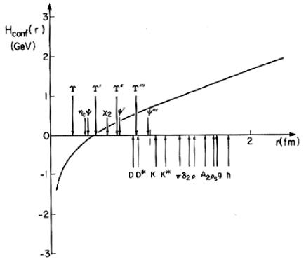
Figure 1: The $q\bar{q}$ potential in a colour singlet meson. Also shown is the rms $q\bar{q}$ separation in some representative mesons. From Ref. [1].

Another way of showing this is given in Fig. 2 which plots the regge trajectories of the isovector, strange, and strangeonium mesons on a Chew-Frautschi plot [2]. The masses of the observed high $L$ states fall on these trajectories. The straight line behavior of this plot reflects the linear nature of the confining potential. This can be seen by examining the relativistic Schrodinger-like equation:

$$[\sqrt{p^{2}+m_{q}^{2}}+\sqrt{p^{2}+m_{\bar{q}}^{2}}-\frac{4}{3}\frac{\alpha_{s}}{r}+br+C]|\psi\rangle=E|\psi\rangle.$$ (2)

In the large-$L$ limit this becomes

$$(L/r+br)\psi(r)=E\psi(r)$$ (3)

which has a classical minimum at $r=(L/b)^{1/2}$. Upon substitution this yields $E^{2}=4bL$, the observed behavior.

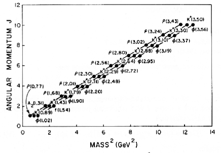
Figure 2: Chew-Frautschi plot for the $\rho$, $K^{*}$, and $\phi$ trajectories. From ref. [2].

2.3 The Spin Dependent Potentials

In addition to the confining potential there are spin dependent pieces of the Hamiltonian. The first piece that we discuss is the hyperfine interaction which includes a contact piece and a tensor piece. It arises from colour-magnetic interactions originating in the short range one-gluon-exchange in analogy to similar effects in atomic physics originating in QED. The hyperfine Hamiltonian is given by the following equation:

$$H_{ij}^{hyp}=\frac{4\alpha_{s}(r)}{3m_{i}m_{j}}\left\{\frac{8\pi}{3}\vec{S}_{i}\cdot\vec{S}_{j}\delta^{3}(r_{ij})+\frac{1}{r_{ij}^{3}}\left[\frac{3\vec{S}_{i}\cdot\vec{r}_{ij}\vec{S}_{j}\cdot\vec{r}_{ij}}{r_{ij}^{3}}-\vec{S}_{i}\cdot\vec{S}_{j}\right]\right\}$$ (4)

It is responsible for the ${}^{3}S_{1}-^{1}S_{0}$ splittings; for example the $\rho-\pi$, $K^{*}-K$, $D^{*}-D$, and $J/\psi-\eta_{c}$ splittings. The short range nature of the contact interaction is supported by the small splittings between the centre of gravity of the ${}^{3}P_{J}$ and the ${}^{1}P_{1}$ multiplets. For P-waves the wavefunction at the origin is zero so that the expectation value of the $\delta$-function in the contact term is zero. If the $\vec{S}\cdot\vec{S}$ term were long range one would expect splittings between the ${}^{3}P_{J}$ and the ${}^{1}P_{1}$ multiplets of the same order as the ${}^{3}S_{1}-^{1}S_{0}$ splittings.

The second spin-dependent contribution is the spin-orbit interaction. There are two contributions to the spin-orbit interaction. The first is a purely relativistic effect. An object with spin moving in a central potential will undergo Thomas precession. This term is given by:

$$H_{ij}^{S.O.(t.p.)} = -\frac{1}{2r_{ij}}\frac{\partial V(r)}{\partial r_{ij}}\left(\frac{\vec{S}_{i}}{m_{i}^{2}}+\frac{\vec{S}_{j}}{m_{j}^{2}}\right)\cdot\vec{L}.$$ (5)

In addition there is a colour magnetic spin-orbit term arising from one-gluon-exchange. This term is given by:

$$H_{ij}^{S.O.(c.m.)} = \frac{4\alpha_{s}(r)}{3r_{ij}^{3}}\left(\frac{1}{m_{i}}+\frac{1}{m_{j}}\right)\left(\frac{\vec{S}_{i}}{m_{i}}+\frac{\vec{S}_{j}}{m_{j}}\right)\cdot\vec{L}.$$ (6)

The spin-orbit Hamiltonian contributes to splittings within ${}^{3}L_{J}$ multiplets for $L\neq 0$. It also contributes to the mixing of ${}^{3}L_{J}-^{1}L_{J}$ states when $m_{q}\neq m_{\bar{q}}$. For unequal mass quark and antiquark $C$-conjugation is no longer a good quantum number and states with different $S$ but the same total $J$ can mix [10, 11]. Note that the two terms contribute with opposite sign. At short distance the colour magnetic contribution with $r^{-3}$ dominates while at large average separation the Thomas precession contribution dominates. Thus, at high orbital (and radial) excitation where the $q-\bar{q}$ pair have on average larger separation, we expect the triplet multiplets to invert relative to the ordering of the low excitation multiplets [12]. By this we mean that $M(^{3}L_{L+1})>M(^{3}L_{L})>M(^{3}L_{L-1})$ at low $L$ while $M(^{3}L_{L-1})>M(^{3}L_{L})>M(^{3}L_{L+1})$ at high $L$. Because the details of this multiplet inversion depend on the confinement potential measuring the masses of excited mesons gives us information about the confinement potential that cannot be obtained elsewhere.

2.4 The Strangeonium Spectrum

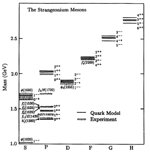
Figure 3: The Strangeonium mass spectrum. The mass predictions come from Ref. [1].

Most of the details we just discussed are summarized in the plot of the strangeonium mass spectrum shown in Fig. 3. The first observation is the regularity of the spectrum. There is good agreement for the masses of the leading orbital excitations which supports the linearity of the confining potential. Extracting the ${}^{3}S_{1}-^{1}S_{0}$ splitting from the $\phi-\eta^{\prime}$ splitting is non-trivial because of the large annihilation mixing between the $0^{-+}$ $ns$ and $s\bar{s}$ components [13, 1]. Nevertheless comparing the ${}^{3}S_{1}-^{1}S_{0}$ to the ${}^{3}P_{J}-^{1}P_{1}$ splittings is consistent with the expected short distance contact interaction arising from one-gluon-exchange. What is striking about this figure is how little information exists about higher orbitally excited and radially excited multiplets. Only the ground state 1S and 1P multiplets are complete and even in the 1P multiplet questions exist. As has been pointed out already, the study of the properties of these mesons can yield a better understanding of the underlying theory. As to the problems alluded to, one notes that there are currently two candidates for the ${}^{3}P_{1}$ state, the $f_{1}/E(1420)$ and the $f_{1}^{\prime}(1530)$. There is an ongoing discussion in the literature about the true nature of these states [14]. In addition, one notes the existence of the $f_{J}/\theta(1720)$ [15]. Although it is not considered to be a candidate for the 1P $s\bar{s}$ multiplet it does not fit into the predicted $s\bar{s}$ spectrum. Speculation exists in the literature as to whether this state may be a glueball [16] or perhaps a $VV$ molecule (vector meson-vector meson) [17]. We can conclude that until much more is known about the $s\bar{s}$ spectrum we cannot say that we truly understand the $s\bar{s}$ mesons.

2.5 Additional Comments on Quark Model Predictions

In the previous sections I gave the conventional quark modeller’s view about the meson spectrum. Before proceeding I think it is important to introduce additional effects whose study is still in its infancy. The first of these effects is to include coupled channel effects in the study of mesons. In the simplest example Weinstein [5] has shown that the multiplet degeneracy (ignoring spin dependent interactions) can be broken by coupling the $q\bar{q}$ Hamiltonian to a meson-meson scattering Hamiltonian. The coupling between the $q\bar{q}$ channel and the meson-meson channel is included via a $MM\leftrightarrow q\bar{q}$ transition operator. The coupled channel Hamiltonian is given by:

$$\left(\begin{array}[]{cc}H_{AB}(r_{AB})&V_{AB\leftrightarrow R}(r_{AB})\\ V_{AB\leftrightarrow R}(r_{AB})&H_{S}{R_{q\bar{q}}}(r_{q\bar{q}})\end{array}\right)$$ (7)

The different $J$ dependent angular momentum terms in $H_{MM}$ gives rise to shifts in the resonance pole resulting in multiplet splitting. Weinstein’s results for the strange P-wave mesons are given in Fig. 4. The scattering curves for the $K_{0}$ and $K_{2}$ are obtained in $K\pi$ scattering while the $K_{1}$ curve is obtained from $K^{*}\pi$ scattering. A complete analysis would of course include both spin dependent interactions in $H_{q\bar{q}}$ and all channels that could couple to the quantum numbers being studied. Such a study may, for example, explain the strange axial meson mixing and the discrepancy between the quark model predictions and experimental measurements of the exicted $\rho$ meson properties.

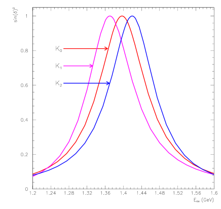
Figure 4: Resonance masses of the strangeness $\pm 1$, $\ell{q\bar{q}}=1$, $S{q\bar{q}}=1$, $J=0,\;1,\;2$ triplet as $J$ varies. The $K_{0}$ and $K_{2}$ are obtained from the $S-$ and $D-$wave scattering of $K\pi$ respectively while the $K_{1}$ is obtained from $s-$wave scattering of a $K^{*}\pi$ pair. From Ref. [5].

The second effect that might potentially make an important contribution to meson properties is the contribution of final state interactions. These may have an effect on the widths calculated in a hadron decay model but they should also be included in coupled channel calculations like those described above. Ultimately one wants to perform a calculation that resembles as closely as possible what is measured by an experiment. A systematic analysis of mesons which includes these contributions would clearly be a useful addition to the subject.

2.6 Summary of Mesonic States

Our knowledge of light meson spectroscopy is summarized in Fig. 5. Note that most radial and orbital excitations are missing. This question must be addressed but it is likely due to a number of reasons. In some cases the states are simply not produced in channels that have been easily accessable experimentally. In other cases the states are too broad to be easily seen while in still other cases, although the states are not too broad, they decay via broad isobars making it difficult to reconstruct the resonance.

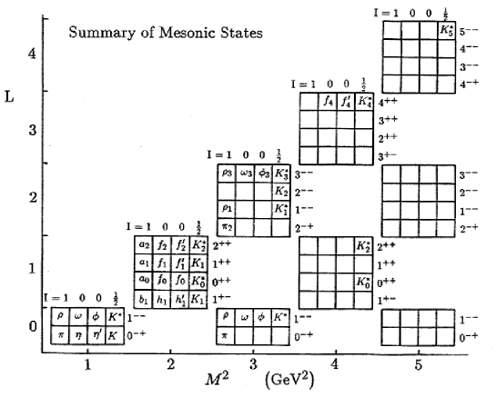
Figure 5: Summary of mesonic states with light quarks.

In addition to the question of missing states there are numerous longstanding puzzles. Some of these are:

$\eta/\iota(1440)$

The $\eta(1440)$ is seen in $J/\psi$ radiative decay and is observed to decay with a large partial width to $\gamma\rho$. This implies that it is a mainly $ns$ radial excitation of the $\eta$. However, another candidate for the mainly $ns$ radial excitation is the $\eta(1295)$. Recent measurements suggest that the $\eta(1440)$ may be split into two $0^{-+}$ states.

$f_{1}/E(1440)$

This state was first reported in 1980. It was regarded to be the $1^{++}$ $s\bar{s}$ state. Since then there have been a number of observations of an axial meson with mass around 1510 Mev. The higher mass is more consistent with the $s\bar{s}$ P-wave multiplet than the $f_{1}(1440)$ mass. As a consequence there is speculation that the $f_{1}(1440)$ is a hybrid, a four-quark state, or a $K^{*}\bar{K}$ bound state [18]. Because of its closeness in mass to the $\eta(1440)$ it is possible that the two states share a common origin.

$f_{J}/\theta(1710)$

This state is seen in the gluon rich $J/\psi$ radiative decay in the $K\bar{K}$ final state but it is not seen in $K\bar{K}$ by the LASS collaboration. It is either spin 0 or spin 2. Its mass is not consistent with quark model expectations for a state with these quantum numbers and as a result is considered to be a prime glueball candidate [16] although, as already mentioned, another explanation is that it is a $VV$ molecule [17].

$J^{PC}=0^{++}$

There are many more scalar mesons than can be accomodated as $q\bar{q}$ resonances. For a long time the $a_{0}(980)$ and $f_{0}(980)$ were believed to be the isovector and $ns$ isovector members of the ground state scalar meson nonet. However, the properties of these states were substantially different from the quark model predictions [1] but were consistent with their interpretation as $K\bar{K}$ molecules analogous to the deuteron bound state [19]. With observation of the $a_{0}(1450)$ by the Crystal Barrel collaboration and the explanation of the $\pi\pi$ S-wave phase shift by the existence of (at least) the $f_{0}(980)$ and $f_{0}(1370)$ the $K\bar{K}$ molecule interpretation is reinforced.

$f_{0}(1500)$

This state has been reported by the ASTERIX, Crystal Barrel, and GAMS Collaborations. Because of its relatively narrow width, its decay properties, and the fact its mass is consistent with lattice gauge theory glueball mass calculations [16, 20] the $f_{0}(1500)$ is considered to be a prime glueball candidate.

$J^{PC}=2^{++}$

The two $1^{3}P_{2}$ $q\bar{q}$ isoscalar states are most certainly the well known $f_{2}(1270)$ and $f_{2}^{\prime}(1525)$. Numerous additional tensor mesons have been observed which have been suggested to be non-$q\bar{q}$ states: the $f_{2}(1430)$, $f_{2}(1520)$, $f_{J}(1710)$, $f_{2}(1810)$, etc [21]. Clearly considerable work is needed to understand the nature of the mesons reported in this sector.

In addition, recent data gives hints of new states; the $a_{1}(1700)$ and the $\pi(1800)$. There has been some speculation as to whether these are conventional $q\bar{q}$ resonances or hybrids [22, 23]. To distinguish the possibilities more data is needed.

To make progress in unravelling the meson spectrum by finding the missing states and solving some of these puzzles will take unprecedented statistics to perform the necessary partial wave analysis to filter the $J^{PC}$ quantum numbers. In addition, techniques will have to be developed to study broad resonances, both theoretical and experimental.

3 Meson Decays

To test our understanding of mesons we have to go beyond a comparison of mass predictions and probe mesons’ internal structure. Because decays are sensitive to the details of the meson wavefunctions they are an important test of our understanding of the internal structure of mesons. In addition, it is important to know the expected decay modes for meson searches. As was already mentioned, knowing something about the expected decay properties might explain why they are missing. Finally, comparing the observed decay properties of mesons to the expectations of different interpretations, $g\bar{q}$ vs hybrid for example, is an important means of determining what they are.

3.1 Decay Models

A number of models exist in the literature; the pseudoscalar emmission model, the ${}^{3}P_{0}$ model, and the flux-tube breaking model [24]. These decay models all give good overall results but there can be large variations in individual decay rates depending on the specific assumptions of the calculation. The results of a fit to well known decay widths are shown in Fig. 6.

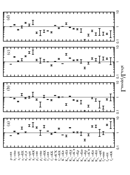
Figure 6: The ratio of decay model predictions for partial widths to the experimental values. The error bars only include the effects of experimental errors in the ratios. (a) and (b) correspond to variations of the ${}^{3}P_{0}$ model using SHO wave functions. (c) and (d) correspond to variations of the flux-tube-breaking model using the wavefunctions of Ref. [1].

3.2 The $\xi(2220)$: Strong Decays of the $1^{3}P_{2}$ and $1^{3}P_{4}$ $s\bar{s}$ Mesons

The $\xi(2220)$ is an interesting example of the approach one takes to understand the nature of a new resonance. The $\xi(2220)$ was discovered in $J/\psi$ radiative decay by the MARK III collaboration. It was found to be very narrow so on this basis it was assumed to be something exotic as conventional wisdom believed that a high mass conventional meson should be relatively broad. Another interpretation pointed out that it could be an $s\bar{s}$ state as its masses were consistent with the masses predicted for the $1F$ $s\bar{s}$ mesons [25]. A quark model calculation found the ${}^{3}F_{J}$ $s\bar{s}$ widths to be relatively narrow because these states have a limited number of decay modes which were calculated to be relatively narrow. Unfortunately this study was not exhaustive and neglected decays to $L=1$ mesons under the assumption that with very little phase space these decay modes should be narrow. The more important decays from a recent, more complete calculation, are given in Table 2 [26].

Table 2: Decay widths (in MeV) for the ${}^{3}F_{4}$ $s\bar{s}$ and ${}^{3}F_{2}$ $s\bar{s}$ states. From Ref. [26].

Decay	${}^{3}P_{0}$(KIPSN)
$f^{\prime}_{4}\to[K\bar{K}]_{0,G}$	29
$f^{\prime}_{4}\to[K^{*}(892)\bar{K}+c.c.]_{1,G}$	27
$f^{\prime}_{4}\to[K^{*}(892)\bar{K}^{*}(892)]_{2,D}$	44
$\sum_{i}\Gamma_{i}$	132
$f^{\prime}_{2}\to[K\bar{K}]_{0,D}$	12
$f^{\prime}_{2}\to[K^{*}(892)\bar{K}+c.c.]_{1,D}$	26
$f^{\prime}_{2}\to[K_{1}(1270)\bar{K}+c.c.]_{1,P}$	187
$f^{\prime}_{2}\to[K_{1}(1270)\bar{K}+c.c.]_{1,F}$	11
$f^{\prime}_{2}\to[K_{2}^{*}(1430)\bar{K}+c.c.]_{2,P}$	24
$f^{\prime}_{2}\to[K^{*}(892)\bar{K}^{*}(892)]_{2,G}$	12
$f^{\prime}_{2}\to[K_{1}(1270)\bar{K}^{*}(892)+c.c.]_{1,P}$	40
$f^{\prime}_{2}\to[K_{1}(1270)\bar{K}^{*}(892)+c.c.]_{2,P}$	13
$f^{\prime}_{2}\to[f_{1}(1510)\eta]_{1,P}$	22
$\sum_{i}\Gamma_{i}$	391

Including the previously neglected decay modes gives a much larger width for the ${}^{3}F_{2}$ state. The ${}^{3}F_{4}$ width, although wider than the observed width, is still consistent within the large uncertainties of the model. The dominant decay modes are to a pseudoscalar meson and a P-wave meson. One can immediately see from Table 2 the reason for this. When ${}^{3}F_{4}$ decays to S-wave mesons they are in a relatively high angular momentum state with the commensurate angular momentum barrier. In contrast, when the ${}^{3}F_{4}$ decays to an S-wave and P-wave meson, the angular momentum can be obsorbed as internal orbital angular momentum so that the mesons are emitted in a lower relative angular momentum state with the corresponding smaller angular momentum barrier. The issues of phase space is relevant comparing the width of the $K_{1}(1270)$ to the width to the $K_{1}(1400)$. The lesson from this example is that it is extremely important to do a complete analysis which in this case means including all allowed decay modes in the calculation.

Recently the BES collaboration has reported measurements of this state with flavour symmetric decays [27]. If these results are confirmed they would reinforce the glueball explanation of this state.

3.3 Additional Comments on Meson Decays

We now have reasonably reliable tools for calculating decay widths which can be used to both understand the nature of new states and predict the most promising channels to search for the missing states [24, 22, 23]. In the former case the models are reasonably reliable, although not totally infallible, and could be used to distinguish between a conventional or hybrid description of a new resonance. For example there are both conventional $q\bar{q}$ and hybrid predictions of an $\eta_{2}$ $J^{PC}=2^{-+}$ state around 1900 MeV. By comparing the predicted partial widths in both scenarios to observed widths one can distinguish between the two scenarios.

	$\rho\rho$	$\omega\omega$	$f_{2}\eta$	$a_{0}(1450)$	$a_{1}\pi$	$a_{2}\pi$	$K^{*}K$
$\eta_{2}(1D)$	147	46	45	1	43	264	61
$\eta_{2}(H)$	0	0	20	2	0	160	10

The interesting channels are the $\rho\rho$, $\omega\omega$, and $a_{1}\pi$ in which the $\eta_{2}(1D)$ has a large partial width while the $\eta_{2}(H)$ has a zero branching fraction. Thus by looking in many different decay channels one can distinguish between the two possibilities.

For excited mesons we should expect cascade decays resulting in many particles in the final state. For example:

$$1F \to 1D+\pi$$ (10)

$$\quad\searrow 1P+\pi$$

$$\quad\quad\searrow 1S+\pi$$

It will therefore be necessary to be able to reconstruct the initial resonance from the complicated many body final state. An additional complication is that some of the intermediate states in the chain are likely to be broad. It will be necessary to understand how to deal with this non trivial problem.

4 Meson Photoproduction

Before concluding I would like to make a few comments about meson production with intense high energy photons which offer a number of photoproduction mechanisms to produce mesons.

Diffractive

This process is likely to be one of the more interesting production mechanisms. It takes advantage of the vector meson content of the photon which can be described by vector meson dominance. The vector meson can be excited into an excited state via pomeron exchange while the target remains in its ground state. What makes this process so interesting is that the photon has a relatively large $s\bar{s}$ content so that photoproduction offers the possibility of producing large numbers of excited $s\bar{s}$ mesons. In some sense we can therefore regard the photon as a $\phi$ beam. The $s\bar{s}$ mesons offer an intermediate step extrapolating from the $c\bar{c}$ states where we have some confidence in the quark model to light quark systems where the model is suspect.

Inelastic

This process is a variation of the previous process except here the target is excited via, say, $\pi$ exchange.

Charge Exchange

This process is also similar except now the exchange particle is charged.

Two Photon

Here a photon is exchanged from the target and fuses with the incident photon to form the final state meson. The two photon couplings offer one more piece of information that can be used to understand the nature of an observed state.

A number of photoproduction experiments have demonstrated the potential of this approach and have made intriguing observations; SLAC hybrid facility, CERN $\Omega$ sepctrometer, FNAL 687, and HERA. Clearly a dedicated facility with a high event rate has much to contribute to the subject.

There are a number of issues that should be addressed. A better theoretical understanding of photoproduction is necessary for planning experiments. To this end, a useful starting point would be to survey the current state of theory. This should be followed by new calculations. A second topic needed to be dealt with as part of detector design is to consider what the signal will look like. The decay models find that high L mesons will likely cascade down to L-1 in steps leading to a large number of particles in the final state. Work should be started on theorist’s simulations which can be fed into detector simulations.

4.1 $\gamma\gamma\to M$

Finally, I want to finish with some comments on two photon production of mesons. As was just stated, two-gamma couplings offer a useful probe of the internal structure of mesons [28]. The observation of a large $\gamma\gamma$ width for the ${}^{1}D_{2}$ $q\bar{q}$ state $\pi_{2}$ suggests that the $\gamma\gamma$ couplings of many orbitally excited light-quark $q\bar{q}$ states may be experimentally accessible. $\gamma\gamma$ couplings could also be crucial in establishing or refuting candidate gluonic mesons or other exotic candidates. There are a number of non $q\bar{q}$ candidates that have been studied in this context; $f_{0}(975)$, $a_{0}(980)$, $\eta(1440)$, $f_{2}(1720)$, and the $\xi(2220)$.

The $\xi(2220)$ provides a timely example. One typically expects $\Gamma_{\gamma\gamma}(M_{q\bar{q}})\sim 1$ keV. ($\Gamma_{\gamma\gamma}(\pi_{2}(1D))\sim 0.1$ keV, ($\Gamma_{\gamma\gamma}(\pi_{4}(1G))\sim 1$ keV). Recently the CLEO collaboration published a result placing the limit of $\Gamma_{\gamma\gamma}B_{KK}(\xi(2220))\leq 1.3$ eV which gives $\Gamma_{\gamma\gamma}\leq 5$ eV [29]. This small two-photon width is much smaller than expected from quark model calculations and is another indication of the non-$q\bar{q}$ nature of the $\xi$.

5 Concluding Comments

In this cursory overview of light $q\bar{q}$ resonances we have seen that the constituent quark model generally gives a good description of light meson spectroscopy. However, there are far too many missing states, especially radial and orbital excitations, and there are numerous puzzles that may point to physics beyond this simple picture of hadron spectroscopy. Until we make progress on both fronts, by observing some of the missing states and making detailed measurements of the states in question, we cannot say that we fully understand hadron physics. To make progress in hadron model building we need to find many states, both conventional and exotic to test and refine our models. This will take unprecedented statistics to perform detailed partial wave analysis that can distinguish between the many different contributions to the cross section at high energy. In addition theoretical progress is needed to understand exactly what is measured by experiment. Some of the topics that need further study are coupled channel effects and final state interactions. In addition it is time that the various production mechanisms be better understood. Effort needed towards the goal of building a dedicated meson spectrometer facility is a better understanding of event rates signals.

There is a compelling case for a dedicated meson spectroscopy facility. The next step is to put the theoretical predictions in a form that is most useful to experimentalists with the goal of designing a detector.

References

- [1] S. Godfrey and N. Isgur, Phys. Rev. D32, 189 (1985).
- [2] S. Godfrey, Phys. Rev. D31, 2375 (1985).
- [3] S. Godfrey and N. Isgur, Phys. Rev. D34, 899 (1986).
- [4] S. Capstick and N. Isgur, Phys. Rev. D34, 2809 (1986).
- [5] J. Weinstein, [nucl-th/9606037].
- [6] E. Swanson, Annals Phys. 220, 73 (1992); T. Barnes and E. Swanson, Phys.Rev. D46, 131 (1992).
- [7] P. Geiger and N. Isgur, Phys.Rev. D47, 5050 (1993).
- [8] P. Geiger and E. Swanson, Phys.Rev. D50, 6855 (1994).
- [9] S. Perantonis and C. Michael, Nucl. Phys. B347, 854 (1990).
- [10] S. Godfrey and R. Kokoski, Phys. Rev. D43, 1679 (1991).
- [11] H. Blundell, S. Godfrey, B. Phelps, Phys. Rev. D53, 3700 (1996).
- [12] S. Godfrey, Phys. Lett. 162B, 367 (1985).
- [13] N. Isgur, Phys. Rev. D12, 3770 (1975); A. De Rujula, H. Georgi and S.L. Glashow, Phys. Rev. D12, 147 (1975).
- [14] See for example, T. H. Burnett and S.R. Sharpe, Ann. Rev. Nucl. Part. Sci. 40, 327 (1990).
- [15] C. Edwards et al., Phys. Rev. Lett. 48, 458 (1982).
- [16] J. Sexton et al., Phys. Rev. Lett. 75, 4563 (1995).
- [17] K. Dooley, E.S. Swanson, and T. Barnes, Phys. Lett. 275B, 478 (1992);
- [18] D. Caldwell, Mod. Phys. Lett. A2, 771 (1987).
- [19] J. Weinstein and N. Isgur, Phys. Rev. D27, 588 (1983); Phys. Rev. Lett. 48, 659 (1982); D41, 2236 (1990); J. Weinstein, Phys. Rev. D47, 911 (1993).
- [20] G. Bali et al., Phys. Lett. B309, 378 (1993);
- [21] Particle Data Group, R.M. Barnett et al., Phys. Rev. D54, 1 (1996).
- [22] T. Barnes, F.E. Close, P.R. Page, and E.S. Swanson, Phys.Rev. D55, 4157 (1997).
- [23] F.E. Close and P.R. Page, Phys.Rev. D56, 1584 (1997).
- [24] R. Kokoski and N. Isgur, Phys. Rev. D35, 907 (1987); E.S. Ackleh, T. Barnes, and E.S. Swanson, Phys. Rev. D54, 6811 (1996).
- [25] S. Godfrey, R. Kokoski, and N. Isgur, Phys. Lett. B141, 439 (1984).
- [26] H. Blundell and S. Godfrey, Phys. Rev. D53, 3700 (1996).
- [27] BES Collaboration (J.Z. Bai et al.), Phys. Rev. Lett. 76, 3502 (1996).
- [28] Z.P. Li, F.E. Close, and T. Barnes, Phys. Rev. D43, 216 (1991).
- [29] CLEO Collaboration (R. Godang et al.), Phys. Rev. Lett. 79, 3829 (1997) [hep-ex/9703009].