MPI-PhE/97-33
hep-ph/9712505
December 1997
QCD and the Hadronic Final
State in Deep Inelastic Scattering at HERA
Michael Kuhlen
Max-Planck-Institut für Physik
Werner-Heisenberg-Institut
Föhringer Ring 6
D-80805 München
Germany
E-mail: kuhlen@desy.de
Abstract
The measurements of the hadronic final state in deep inelastic scattering at HERA are reviewed and discussed in the context of QCD. Covered are the general event properties in terms of energy flows, charged particle production, and charm and strangeness production. Quark fragmentation properties are studied in the Breit frame. Event shape measurements allow “power corrections” to be applied and the strong coupling to be extracted. Other measurements are based on dijet rates. Jet rates as well as charm production have been used to determine the gluon density in the proton. Indications have been found in the hadronic final state for unconventional, non-DGLAP evolution at small , which could be explained with BFKL evolution. Signatures for QCD instanton effects are discussed and first search results are presented.
Habilitationsschrift, submitted to Universität Hamburg in December 1997
The measurements of the hadronic final state in deep inelastic scattering at HERA are reviewed and discussed in the context of QCD. Covered are the general event properties in terms of energy flows, charged particle production, and charm and strangeness production. Quark fragmentation properties are studied in the Breit frame. Event shape measurements allow “power corrections” to be applied and the strong coupling to be extracted. Other measurements are based on dijet rates. Jet rates as well as charm production have been used to determine the gluon density in the proton. Indications have been found in the hadronic final state for unconventional, non-DGLAP evolution at small , which could be explained with BFKL evolution. Signatures for QCD instanton effects are discussed and first search results are presented.
Chapter 1 Introduction
1.1 Overview
Motivation
HERA111“Hadron-Elektron-Ring-Anlage” is the world’s first electron222 HERA can operate with either electrons or positrons. In the following, the generic name electron is used for electrons as well as for positrons.-proton collider. The large centre of mass (CM) energy of 300 GeV allows to explore new regimes: new particles with masses up to 300 GeV can be produced, the structure of the proton can be studied with a resolving power varying over 5 orders of magnitude down to dimensions of m, and partons with very small fractional proton momenta (Bjorken down to ) become experimentally accessible. The hadronic final state which emerges when the proton breaks up has an invariant mass up to 300 GeV. It provides a laboratory to study quantum chromodynamics (QCD) under varying experimental conditions, which can be controlled by measuring the scattered electron. The hadronic final state carries information on the structure of the proton. It is made use of to study the dynamics of the proton’s constituents, complementary to structure function measurements.
In contrast to “clean” interactions, the initial state in collisions contains already a strongly interacting particle. That makes the physics more complicated, but leads also to interesting effects that cannot be studied in collisions. At HERA, well established fields are being studied, exploiting the tunable kinematic conditions. These comprise jet physics and comparisons with perturbative QCD to extract the strong coupling and the density of gluons in the proton, or for example the measurement of fragmentation functions. Other topics have only blossomed with the advent of HERA. To name a few, a class of events with large rapidity gaps and small physics allow longstanding problems in QCD to be addressed, which are connected with scattering cross sections at high energies and confinement. There are also exotic effects like instanton induced reactions, which, if discovered at HERA, would alter significantly our view of particle physics.
Purpose
This work provides a review of the hadronic final state measurements at HERA in deep inelastic scattering (DIS). The emphasis is on experimental results, because in many cases at HERA, experiment is driving theory. Many measurements are being performed without any theoretical prediction, and often they have not yet found an unambiguous theoretical explanation. Nevertheless, the results are discussed in the context of the theory, where possible.
The review of the experimental situation is complete up to the fall of 1997. It can therefore be consulted for quick access to the HERA data. Basic concepts are explained in a partly pedagogical fashion to serve physicists from outside the HERA community and newcomers to HERA physics.
Contents
In chapter 1 the HERA machine and the H1 and ZEUS experiments are introduced, and the kinematic variables are discussed. In chapter 2 the theoretical framework of deep inelastic scattering is set up with evolution equations and a special section on the interest in small physics. The hadronic final state should not be discussed without knowledge of the inclusive cross section and the proton structure functions (chapter 3). In chapter 4 we start with simple models for hadron production. They are subsequently being refined in chapter 4 and serve as the basis for the discussion of the data.
Measurements of basic event properties are presented in chapter 5: energy flows, charged particle spectra, charm and strangeness contents, Bose-Einstein correlations. The fragmentation of the scattered quark is studied in chapter 6 and compared with quark fragmentation in annihilation and QCD calculations. Measurements of event shape variables allow a new view on hadronziation properties with “power corrections”, offering a potentially powerful tool for measurements of the strong coupling . Jet production has been compared to perturbative QCD predictions to measure and the gluon density in the proton (chapter 7). By measuring jet rates, regions of phase space have been identified where the measured jet rates are not well understood yet, and where the underlying physics is possibly departing from the conventional picture of deep inelastic scattering.
Also the energy flow measurements at small have not yet found an unambiguous theoretical interpretation. In chapter 8 on low physics dedicated searches for “footprints” of new QCD effects (BFKL) are discussed: energy flows, high particles and “forward jets”. Chapter 9 deals with the possibility to discover QCD instantons at HERA, which would have far reaching consequences for our understanding of field theories and for cosmology.
Some related topics and neighbouring fields could only be touched upon. The interested reader is referred to other reviews on structure functions [1, 2], rapidity gaps [3], photoproduction [4] and on hadron production at fixed target experiments [5].
Throughout, unless stated otherwise, the data shown have been corrected for detector effects and QED radiation, and the errors comprise statistical and systematic errors added in quadrature.
1.2 The HERA Machine
In the HERA machine, electrons and and protons are accelerated and stored in two separate rings. The circumference of the machine is 6.3 km. The magnets of the proton ring are superconducting, the magnets of the electron ring are conventional. The final beam energies are for electrons and for protons with a collision centre of mass energy of . Early data were collected with .
The beams are collided head-on in two interaction regions occupied by the experiments H1 and ZEUS. There are 220 bunch positions in the beam, of which typically 190 are filled with a few particles per bunch. The time between bunch crossings is 96 ns. The longitudinal bunch length is about 60 cm, leading to an approximately Gaussian distribution of interaction points along the beam line with width 10 cm. The transverse beam size is 300 m horizontally by 70 m vertically.
In 1997 the average peak luminosity was with average beam currents at the beginning of a fill of 77 mA for protons and 36 mA for electrons. The total integrated luminosity for the 1997 run was 35 . Most analyses in this review are based on data from the runs 1992-1994, corresponding to an integrated luminosity of .
1.3 The H1 and ZEUS Detectors
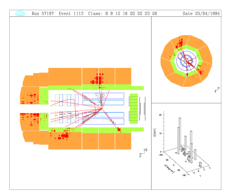
The H1 [6, 7] and ZEUS detectors [8] serve to detect the scattered electron in collisions and to measure the emerging hadrons. The individual detector components are mounted concentrically around the beam line. Due to the asymmetric beam energies, the hadronic system is boosted into the proton direction (). Therefore the detectors are also asymmetric with respect to the interaction point, with enhanced instrumentation for hadrons in the (forward) direction. The acceptances and resolutions of the main detector components for the analyses presented here are given in table 1.1. Fig. 1.1 shows a drawing of the ZEUS detector, and fig. 1.2 an event display from H1.

| H1 | ZEUS | |||
| tracking | acceptance | resol. | acceptance | resol. |
| forward | ||||
| central | ||||
| calorimetry | acceptance | resol. | acceptance | resol. |
| electromagnetic | (LAr) | (U) | ||
| (BEMC) | ||||
| (SPACAL) | ||||
| hadronic | (PLUG) | |||
| (LAr) | (U) | |||
| (SPACAL) | ||||
Closest to the beam line are wire chambers for measuring charged particle trajectories. The particles’ momenta are determined from their track curvature in a longitudinal magnetic field provided by a superconducting coil.
Electromagnetic and hadronic showers are measured in calorimeters surrounding the inner tracking devices. H1 emphasizes electron detection with a finely segmented lead (inner electromagnetic part) and steel (outer hadronic part) liquid argon calorimeter (LAr) with good energy resolution for electrons, supplemented by a dedicated electromagnetic backward calorimeter. From 1992-1994 an electromagnetic lead/scintillator sandwich calorimeter was installed in the backward region (BEMC), and from 1995 onwards a lead/scintillating fibre calorimeter (SPACAL). A copper calorimeter with silicon readout (PLUG) covers part of the forward beam hole. Compensation for the different response to hadronic and electromagnetic showers in the LAr is done offline by a software weighting technique. ZEUS achieves better hadronic energy resolution with a self-compensating uranium/scintillator calorimeter (U), and compromises on electromagnetic energy resolution.
The calorimeters are surrounded by chambers and absorber plates for measuring shower leakage and for muon detection. Further specialized detectors are installed very close to the beam line to detect particles that are scattered under small angles. Silicon detectors that have already been installed as vertex detectors or are being planned have not yet been used in physics analyses.
1.4 Kinematics
Definition of kinematic variables
The kinematics of the basic scattering process in Fig. 1.3 can be characterized by any set of two Lorentz-invariants out of and , which are built from the 4-momentum transfer mediated by the virtual boson and from the 4-momentum of the incoming proton. The invariant mass squared is . These kinematic variables are then:
| (1.1) |
which gives the transverse resolving power of the probe with wavelength (we set );
| (1.2) |
the Bjorken scaling variable (), which can be interpreted as the momentum fraction of the proton which is carried by the struck quark (in a frame where the proton is fast, and assuming the quark-parton model to be a good approximation);
| (1.3) |
the transferred energy fraction from the electron to the proton in the proton rest frame (); and
| (1.4) |
the invariant mass squared of the outgoing hadronic system . The invariant
| (1.5) |
is rarely used at HERA. In the proton rest frame it gives the energy transfer from the lepton to the proton.

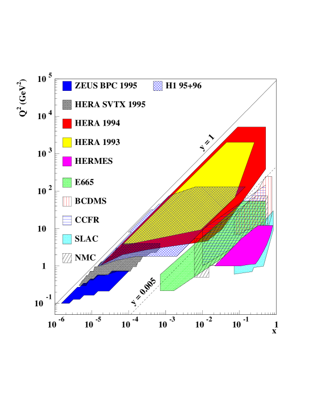
The large CM energy gives access to kinematic regions both at very small and at large (Fig. 1.4). The HERA data cover roughly , and .
Experimental reconstruction of the event kinematics
The kinematics can be determined either from the electron alone, or from the measured hadronic system alone, or from a combination of both, permitting important systematic cross checks. The hadronic measurement relies mostly upon the calorimeters. At large the precision of the hadron method can be improved by momentum measurements in the trackers.
- The electron method
-
The kinematic variables are calculated from the energy and angle of the scattered electron (measured with respect to the proton direction):
(1.6) - The hadron method
-
The kinematics is measured entirely with the hadronic system:
(1.7) Here and denote the 4-vector components of the hadronic system , which are calculated as the 4-momentum sum over all final state hadrons . Jacquet and Blondel [9] have shown that the contribution from hadrons lost in the beam pipe is insignificant.
- The Sigma method [10]
-
Here the denominator of is replaced with , where runs over all final state particles, including the scattered electron. This expression equals due to energy momentum conservation. In case the incident electron had radiated off photons which escape detection, the sum yields the true electron energy which goes into the interaction. This method relies on both electron and hadron measurements. With
(1.8) where the sum runs over all hadronic final state particles, the kinematic variables can be written as
(1.9) The denominator is twice the energy of the “true” incident electron, after QED radiation from the incoming electron beam.
- The double angle method
-
We define the angle by
(1.10) In the simple quark parton model would be the angle of the scattered (massless) quark. The kinematic variables can be calculated from regardless of its interpretation:
(1.11) and
(1.12)
For most of the phase space the electron method is superior. At small the hadron method has a better resolution than the electron method. The “mixed method” uses reconstructed from the electron method and reconstructed with the hadron method. Also the double angle method and the sigma method use information from both the electron and the hadronic system, thus interpolating between the pure electron and hadron methods. The sigma method has the advantage that it corrects for initial state radiation.
Chapter 2 Theoretical framework
2.1 Deep Inelastic Scattering
The fundamental measurement in DIS concerns the cross section for as a function of the kinematic variables (any pair of two independent ones). The quark parton model (QPM) offers a physical picture: the scattering takes place via a virtual photon which is radiated off the scattering electron, and which couples to a pointlike constituent inside the proton, that is a quark or antiquark. The cross section is then proportional to the quark density inside the proton.
The differential cross section can be expressed in terms of two111For the sake of simplicity, exchange (a 1% correction for ) has been neglected, and the structure function thus been omitted. independent structure functions and :
| (2.1) |
is the electromagnetic coupling constant. Here we have expressed the cross section also in terms of the longitudinal structure function and the ratio , defined as
| (2.2) |
can be interpreted as the ratio of the cross sections and for the absorption of transversely and longitudinally polarized virtual photons on protons, with . The structure function can be expressed222We use the Hand convention [11] for the definition of the virtual photon flux. in terms of and ,
| (2.3) |
where the small approximation has been applied. Similarly,
| (2.4) |
In the “DIS” scheme can be written in terms of the quark and antiquark densities, and , and their couplings to the photon, i.e. their charges :
| (2.5) |
where the sum runs over all quark flavours333 Equation 2.5 represents the “leading twist” (called twist 2) contribution to the structure function , when expanded in powers of [2], (2.6) The coefficients are varying logarithmically with . The “higher twist” terms (, called twist 4, 6 etc.) arise from interactions of the struck parton with the remnant and are suppressed by . We shall not pursue higher twist effects any further, but note that they may not be negligible at small for as large as a few [2, 12].. In other schemes (for example the “” scheme) the relation between and the parton densities (eq. 2.5) holds only in leading order perturbation theory. The longitudinal structure function vanishes in zero’th order , and will be discussed in section 3.3.
In the simple quark parton model the proton consists just of 3 valence quarks. Their distribution functions in fractional proton momentum , , would peak at and tend towards zero for . In a static model of the proton, they would not depend on . It follows that should not depend on , just on (Bjorken scaling).
When QCD is “turned on” the quarks may radiate (and absorb) gluons, which in turn may split into quark – antiquark pairs or gluon pairs. More and more of these fluctuations can be resolved with increasingly shorter wavelength of the photonic probe, . With increasing, we have a depletion of quarks at large , and a corresponding accumulation at lower . In addition, “sea quarks” from splittings populate small . In fact, at small it is the gluon content with distribution function that governs the proton and gives rise to the DIS cross section via the creation of pairs.
2.2 Evolution Equations
It has not yet been possible to calculate the structure of the hadrons from first principles, involving the building blocks of hadronic matter, the quarks and gluons, and their mutual interactions as given by QCD. Therefore also the lepton-nucleon scattering cross section cannot be calculated from first principles. Due to the factorization theorem of QCD one can however split the problem. The cross section can be calculated by folding initial parton distribution functions , giving the density of partons in the proton , with a perturbatively calculable lepton-parton scattering cross section. Symbolically
| (2.7) |
for scattering (see fig.2.1a). The initial parton distributions cannot be calculated. They have to be determined experimentally. They are however universal in the sense that once they have been measured in one reaction, they can be used for calculations of other processes. Rather than employing the rigorous operator product expansion (OPE) technique for the evolution of the structure functions (see e.g. [13]), we shall use in this section the more intuitive picture of Feynman diagram summation.


The expansion parameter for the perturbation series is the strong coupling . The coupling is scale dependent according to the “renormalization group equation” (see [14] for a concise summary). The two-loop expression (next-to-leading order = NLO) for the “running” coupling as a function of the renormalization scale is
| (2.8) |
where
| (2.9) |
The renormalization scale is set by the length scale () over which the interaction takes place, given for example by the virtuality of the probing photon in DIS, or by the of a parton. By eq. 2.8 the QCD scale parameter is introduced. In contrast to , its definition depends on the number of active flavours and on the renormalization scheme (for example the “minimal subtraction scheme” ). The strong coupling decreases with increasing scale – at short distances partons become asymptotically free. grows beyond all bounds for small scales () or large distances, when perturbation theory breaks down and confinement sets in. The size of a hadron 1 fm provides an estimate when that happens. Therefore GeV. The current world average for at the scale set by the mass is or for 5 flavours [14].
The calculation of the cross section is a formidable task. It turns out that there is no fast convergence of the perturbation series (fig. 2.2). Many diagrams contribute and have to be summed up. One encounters two types of divergencies. Divergencies due to the radiation of soft quanta with small momenta are exactly cancelled by virtual corrections to graphs where that radiation is absent (“no emission”). Divergencies due to collinear radiation (so called collinear or mass singularities for ) can be absorbed (factorized off) into the “bare” parton distribution functions. Thereby they are redefined and depend now on the (mass) factorization scale , and so does the electron-parton scattering cross section with the singularities removed:
| (2.10) |
(see fig. 2.1a). The choice of the factorization scale is arbitrary. The physical cross section is of course independent of . Often one chooses , because then reduces to the Born graph (here by exchange, fig. 2.1b). In the parton picture is then interpreted as the parton density in the proton as seen by a photon with virtuality (resolving power) .
 |
 |
 |
|
 |
 |
Since can in principle be calculated perturbatively for any scale, one can also calculate the change of the redefined parton distribution function with a change of scale. These are the evolution equations. Once a parton distribution function (or structure function) is known at one scale, it can be calculated for any other scale. For the derivation of the evolution equations, one has to perform the perturbative calculation of , taking into account all contributing graphs (fig. 2.2). In order to carry out the calculation in practice, one applies certain approximations, thus restricting the phase space for radiation. Such approximations are then valid in regions of and where the selected contributions are the dominant ones. In the following, evolution equations will be discussed which differ in their approximations, and therefore in their regions of validity. Always, in order to allow perturbation theory to be valid, is required.
In a “physical” gauge, in which only the physical transverse gluon polarization states need to be taken into account, the individual contributions of the perturbation series can be represented by so-called ladder diagrams (see fig. 2.3). We work in a frame that moves parallel to the proton, and where the proton is fast. The transverse momenta of the emitted quanta are denoted with . Similarly, the transverse momenta carried by the quanta that constitute the side rails of the ladder are . The longitudinal components are given in fractions of the proton energy and are labelled with for the emitted quanta and with for the internal quanta. Energy-momentum conservation requires , and therefore .

2.3 The DGLAP Equations
In the approximation leading to the DGLAP (Dokshitzer-Gribov-Lipatov-Altarelli-Parisi) equations [15] all ladder diagrams are summed up, in which the transverse momenta along the side rails of the ladder are “strongly ordered”, . This condition implies strong ordering also for the emitted quanta, .
Where can we expect such an approximation to be valid? A good pedagogical discussion can be found in [16]. We shall sketch the main arguments. The evaluation of a ladder diagram with rungs requires integrations over the internal momenta exchanged between rungs of the form
| (2.11) |
where the dots represent functions which depend on the actual nature of the emitted quanta and their dynamics. With strong ordering, the nested integration over all rungs in the ladder can be carried out. The result is an expression . We see that the integration yields large logarithms when the ’s are strongly ordered. They compensate the smallness of . Clearly, since decreases only logarithmically with and is compensated by a logarithmically growing term in , in a perturbative expansion all graphs with rungs up to need to be summed up. (Often the expression “re-summation” is used, because one re-arranges the perturbation series such that the largest terms come first). This is called a leading log approximation (here in ), since each power in is accompanied by the same (maximal) power of . Subleading terms would be .
We expect this to be a good approximation when is large, but is not too small in order not to produce also large logarithms,
| (2.12) |
In this approximation, the evolution equations for the quark density for flavour and the gluon density are
| (2.13) |
These are the famous DGLAP equations [15], describing the scaling violations of the structure functions. They involve the calculable Altarelli-Parisi splitting functions . gives the probability per unit of for parton branchings , and , where the daughter parton carries a fraction of the mother’s () momentum. The splitting functions in LO are given by
| (2.14) |
The singularities for soft emissions are cancelled by virtual corrections to the “no-emission” graphs. This is physical, because arbitrary soft emissions cannot be distinguished from the “no-emission” case444Technically the singularities can be regularized by the following prescription. Replace with , where the “+ - prescription” defines how integrals are to be carried out: (2.15) for any function . A term has to be added to , and a term to . . The coupled integro-differential equations for the quark and gluon densities (eq. 2.13) can be solved, allowing to calculate them for any value of and , once they are known at a particular value for .
A special case for which the DGLAP equations can be solved analytically (see for example [13]) occurs when in addition to the above conditions also strong ordering in is required, . The large logarithmic terms arising from the integration are then of the form , which need to be resummed. This is the double leading log approximation (DLL). It is expected to hold when the DLL terms dominate over the others,
| (2.16) |
This is the case for large and small . At small the parton content of the proton is expected to be dominated by gluons, because is largest when gluons are being produced (). When quarks are neglected, and is approximated, the DGLAP equations can be solved to yield the DLL solution [17]
| (2.17) |
provided the gluon density is not too singular at small (needs to be quantified). At small a fast rise of the gluon density with decreasing is predicted. That is, increases faster than , but slower than for any powers . Apart from these shape restrictions the actual rate of the growth is not predicted, it depends on the “evolution length” from to .
2.4 The BFKL Equation
When is small, but not large enough to reach the DLL regime, the DGLAP approximations cease to be valid. For the limit large and finite and fixed the BFKL (Balitsky-Fadin-Kuraev-Lipatov) [18] equation has been derived. It takes into account diagrams in which the are strongly ordered, . No ordering on is imposed. Large logarithms are thus generated that need to be resummed, leading to the leading log approximation in . The region of validity is
| (2.18) |
The BFKL equation is expressed in terms of the “unintegrated” gluon density , which is related to the usual gluon density by
| (2.19) |
The BFKL equation is an evolution equation in . It is formulated for gluons which dominate at small ,
| (2.20) |
where is the BFKL kernel. can be calculated for any (small) , once it is known at some for all . We note in passing that if one requires strong ordering () when solving eq. 2.20, the DLL result is retained [16].
For fixed the equation can be solved analytically. The result is (in the saddle point approximation)
| (2.21) | |||||
with (for colours and ), and (the Riemann function gives ). specifies the starting point for the evolution. Therefore the gluon density is expected to rise like a power of for decreasing , , faster than the DLL result eq. 2.17. However, the running of and higher order corrections decrease the value of [19].
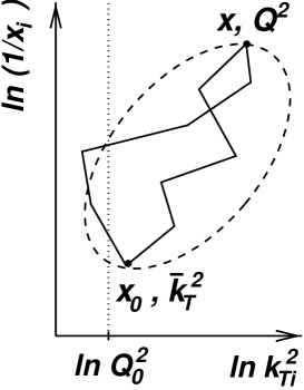
Another characteristic prediction of the BFKL equation is “ diffusion”, in contrast to ordering for DGLAP (see fig. 2.4). The distribution function is Gaussian in with a width that increases with the BFKL “evolution length” . An individual evolution path will follow a kind of random walk in . An ensemble of evolution paths exhibits a diffusion pattern according to the Gaussian in .

diffusion poses a difficulty for the application of the BFKL equation, because may diffuse into the infrared region () where perturbation theory cannot be applied. One therefore usually introduces a lower cut-off for the integration, and studies the dependence of the result on that cut-off. Due to diffusion BFKL looses much of its predictive power when applied to the structure function . The inclusive structure function is probably not a good place to identify BFKL effects unambiguously. It is however possible to study special final state configurations where diffusion into the infrared region can be minimized by fixing both start and end point of the evolution far enough above the infrared region. The search for signs of BFKL evolution in the hadronic final state is presented in chapter 8.
The CCFM equation [20] developed in recent years unifies the BFKL and DGLAP approaches [21] and takes into account coherence effects by angular ordering. The CCFM approach leads to a reduction of the exponent and a reduction of the diffusion [22, 23]. The Linked Dipole Chain model [24] provides an implementation of the CCFM equation which is suited for final state predictions.
2.5 The Interest in Small
Orthogonal evolution equations
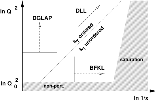
In fig. 2.5 the regions of validity of the different evolution equations are sketched. They are not predicted precisely by the theory, but have to be explored experimentally.
With DGLAP evolution a parton density known for can be evolved to any value of for . The behaviour for cannot be predicted with DGLAP. Similarly, with BFKL evolution a parton density known for can be evolved to any value of . The new feature, orthogonal to the DGLAP evolution, is that the low behaviour is predicted by the theory. In principle DGLAP and BFKL evolution together could be used for a Münchhausen trick (bootstrapping), to predict the structure of the proton for all as long as , above a cut-off to avoid the non-perturbative region. The problem with diffusion into the non-perturbative regime however poses a severe obstacle for that goal to be reached.
Another motivation is connected with the cross section for hadron-hadron scattering at high energies. Before we can make the point, we need to make an excursion to Regge theory (see for example [25] as a review related to HERA physics; [26] and [27] as a modern language textbook introduction; [28] for an in depth discussion of Regge theory).
Regge theory
Consider the elastic scattering of hadrons and , (fig. 2.6a). Their 4-momenta are denoted with for the initial and for the final state. The cross section can be expressed as a function of the Mandelstam variables and . It is the squared sum over the scattering amplitudes due to the quanta (conventionally mesons) that can be exchanged,
| (2.22) |
In Regge theory, where the mesons are connected via a so-called Regge trajectory (explained below), the sum yields
| (2.23) |
is an unknown real function. The complex phase is given by
| (2.24) |
for exchanged particles with parity , and receives an extra factor for negative parity. The Regge trajectory gives the relationship between the mass and the spin of the exchanged mesons, (fig. 2.6b).
Empirically, Regge trajectories can be parametrized as straight lines with
| (2.25) |
is called the intercept (with the ordinate), and the slope of the trajectory. As an example, a Regge trajectory for mesons is shown in fig. 2.6b. Due to the confinement problem, meson trajectories (hadron masses) could not yet be calculated from first principles in QCD.


The total cross section
Starting from the elastic cross section (in principle one has to sum over all Regge trajectories whose resonances can be exchanged in the reaction)
| (2.26) |
we can use the optical theorem, relating the total cross section to the forward scattering amplitude
| (2.27) |
to predict the behaviour of the total hadron-hadron scattering cross section
| (2.28) |
The total cross sections for , , and reactions are plotted as a function of the CM energy in fig. 2.7. Their behaviour is surprisingly similar (and also for other hadron-hadron scattering cross sections like , etc. that are not shown in fig. 2.7 [14]). They fall at small CM energy GeV, and rise towards large energy. All these cross section can be parametrized with the universal ansatz [30]
| (2.29) |
and are process dependent constants, whereas and [14] are universal, process independent constants.
The Pomeron
The fall off at small energies is readily interpreted as due to meson exchange, whose Regge trajectories have an intercept (compare fig. 2.6b; here only trajectories that dominate high energy scattering are shown; other meson trajectories have smaller intercepts and therefore do not contribute much to high energy scattering). Correspondingly, the rise at high energy is attributed to an exchange described by a Regge trajectory with intercept . There exists however no established set of particles with such a Regge trajectory. Nevertheless, the Regge ansatz gives a successful parametrization of the scattering process. Therefore a hypothetical object, the Pomeron is postulated, which has the quantum numbers of the vacuum (electrically and colour neutral, isospin 0 and parity ), and whose exchange is described by the Pomeron trajectory , see fig 2.6b. The object is suspected to be of gluonic nature, perhaps a glue ball. A possible glue ball candidate with in fact would fall on the Pomeron trajectory, see fig. 2.6b. Because , physical states with belonging to the Pomeron trajectory cannot exist. An up-to-date textbook on QCD and the Pomeron is [27].
Deep inelastic scattering at small can be viewed as virtual photon - proton scattering at high energy . We had connected the structure function with the total cross section for scattering,
| (2.30) |
If the total cross section behaviour found for hadron-hadron scattering and real photon-hadron scattering continues to hold for virtual photon-hadron scattering, one expects to rise as with decreasing .
We note that the power growth of the total cross section will eventually violate the Froissart bound [32] for hadron-hadron scattering,
| (2.31) |
where is an unknown constant. The power growth of must be dampened by some mechanism at large energies.
The small behaviour of
At small , will be determined by the dominant gluon content of the proton, because the quarks to which the photon couples are pair created by the gluons. The BFKL prediction for small was
| (2.32) |
The (LO) BFKL expectation for the small behaviour of is . This power growth is faster than the growth expected from eq. 2.17, the DLL approximation.
This situation is very interesting. The experience from total cross sections at high energies would suggest that should rise at small , a behaviour long known and parametrized with the soft Pomeron, but whose origin is not understood from QCD. On the other hand, in the BFKL approximation, QCD does make a prediction for small , which is different from the past experience: should rise much faster, . The DLL expectation is in between. The slow rise is often said to be due to the “soft Pomeron” or the “non-perturbative” Pomeron, or the “Donnachie-Landshoff” Pomeron. The fast rise would be attributed to the “hard”, or “perturbative”, or “Lipatov”, or “BFKL” Pomeron, if one still wants to use the Regge language (see fig. 2.8). Under which conditions will we see which behaviour? How about the transition region? Do HERA data extend into a kinematic regime where the steep rise of predicted by BFKL can be seen? And if a steep rise is to be seen, is it really to be attributed to BFKL dynamics? Some of the answers will be given by the HERA data presented in the next chapter 3 on structure function measurements. It will turn out however that is too inclusive a quantity to resolve the question of BFKL dynamics. The search for specific signatures of BFKL evolution in the hadronic final state is presented in chapter 8.

Ultimately the hope is that the BFKL equation offers a way to approach the confinement problem of QCD. It allows to make predictions for at small , thus for the structure of hadrons at small , something which otherwise has to be assumed as non-perturbative input for the parton densities. It also makes a prediction for the total cross section at high energies, where previously we had just a prediction based upon a parametrization of “soft” phyics, the “soft” Pomeron. That the two predictions do not coincide makes it all the more interesting.
2.6 Hadronic Final States
So far we have developed the theory for the total inclusive cross section, loosely speaking a sum over everything that can happen inside the proton. When the proton is being probed by the virtual photon, one out of all the possible virtual fluctuations in the proton is selected by the measurement process. The remnants of the fluctuations materialize in the hadronic final state and become observable when the proton wave function is projected onto a specific state. Also the scattered quark and radiation thereoff contribute to the hadronic final state. Matters are even more complicated: the distinction between initial state fluctuations and final state radiation may be practical and justifiable in many cases, but is quantum mechanically not rigorous.
QCD predictions for the hadronic final state are in general much more difficult and less rigorous than for the inclusive cross section. On the other hand the hadronic final state can provide much more detailed information on the QCD processes in scattering than just the total cross section.
Different observables and approximations
It depends very much on the final state observable which technique and approximation is appropriate for a theoretical description. For example, for a global event property like the amount of energy on average emitted in a certain solid angle, it may be a good approximation to interpret the parton evolution equations in a probabilistic way555Strictly speaking the evolution equations have been derived for the inclusive cross section. Cancellations between different diagrams are necessary to ensure that the total cross section stays finite. It is therefore not a priori clear to what extent the evolution equations can be used for hadronic final state predictions. . The evolution equations define a cascade of parton emissions (a parton shower) with specified emission probabilities. One has to sum up all emission cross sections, weighted with the energy. Techncially the calculation could be done analytically, numerically, or with a “Monte Carlo” program. Of course such a calculation will only be valid where the approximations are valid that went into the evolution equations.
For less global quantities, one may find that one has selected a piece of the phase space which is unimportant for the total inclusive cross section, and which might have been rightfully neglected in the evolution equations. For example, for the process with high transverse momenta of the quarks, the DGLAP approximation with strong ordering will not be sufficient to describe the cross section accurately. In that case one will instead use the exact, fixed order QCD matrix element for the process to cover the full phase space, and fold it with the probability to find a gluon in the proton. In practice the matrix element will be calculated only to a few orders in perturbation theory, in leading (LO) or next-to-leading order (NLO)666Calculations in next-to next-to-leading order (NNLO) are not yet available for DIS.. In turn, this approximation will be insufficient for our first example, where many parton emissions contribute. This case is hardly covered by the fixed order matrix element (compare section 5.1); in NLO there are at most 3 partons in the final state. The actual implementations of the different perturbative QCD approximations are presented in section 4.4.
A special rôle play “infrared safe” observables. An infrared safe observable does not change its value when an object in the final state (parton, particle, energy cluster, …) is split collinearly into smaller units, or when a soft object is added. Examples for infrared safe observables are collective observables like energy flows and certain event shape and jet observables. A counter example is the total multiplicity. Infrared safety ensures that perturbative predictions can be made without the need to introduce a cut-off parameter against infrared divergencies. This property is also experimentally advantageous, as it does not require to know the particle composition of a certain energy deposition in the detector that is used in the analysis. For example, calorimeter clusters usually do not have a one-to-one correspondence to incident particles.
Event generators
The calculational techniques differ. Some specific final state observables can be calculated analytically (rarely), or numerically with a program. More ambitious are event generators, “Monte Carlo” programs (see section 4.7). They attempt to model event by event the complete final state. Ideally, an ensemble of Monte Carlo generated events would correspond in all aspects to an ensemble of events collected in nature. An intrinsic difficulty with this approach is that the probabilistic generators have to use probabilities, not probability amplitudes. Quantum mechanical interference effects therefore have to be implemented “by hand”, for example by enforcing an angular ordering for parton emissions (see section 4.4).
Hadronization
One of the biggest problems of QCD is to make contact with the real world of hadrons. Perturbative QCD makes predictions for parton cross sections. Observable are hadrons though. The transition from partons to hadrons (“hadronization”) cannot be treated perturbatively, because it happens at a scale where the strong coupling constant becomes large. Non-perturbative QCD can be considered as one of the last frontiers, where new insight into nature can be gained, or as a nuisance, because it hides the beauty and simplicity of the partonic world from direct observation.
In any case, much has been learnt about hadronization from the study of hadron production. This has led to some rather successful phenomenological models to describe hadronization (see section 4.5). Being models, they are not uniquely defined by theory. Rather, they depend to some extent on ad hoc assumptions and parameters which are being adapted to observation. At least the hadronization models are universal and can be used for different kinds of reactions. Probably the most sophisticated model is based on a colour string (a flux tube) that connects coloured partons. When stretched by the separating partons, the string breaks, pulling new pairs from the vacuum. When no more energy is left in the string, colour neutral hadrons are formed.
Chapter 3 Inclusive Cross Sections
3.1 The Structure Function
ZEUS [33, 34, 35, 36] and H1 [37, 38, 39, 40, 41, 42] have measured in a completely new kinematic domain compared with fixed target experiments, most notably towards much smaller values of , and towards much larger . For kinematic reasons the cross section falls (see eq. 2.1). Here we shall concentrate on the region of less than a few thousand , because very little (though not uninteresting [43, 44, 45]) data exist for higher , especially as the hadronic final state is concerned.
In Fig. 3.1 is shown as a function of for fixed values. At scaling is observed – does not depend on . At decreases with due to parton splittings, the products of which are found then at smaller . Therefore increases with for in accord with the qualitative discussion of section 2.1. When plotted as a function of for fixed (fig. 3.2), exhibits a steep rise towards small , which flattens at smaller . The increase signals growing parton densities with decreasing .


From a DGLAP evolution of pre-HERA data this sharp rise could not be predicted a priori, because input distributions at small were not available. (Assuming however valence-like parton distributions at a small scale , a sharp rise at larger was predicted from DGLAP evolution [49].) It was known though that asymptotically for the small behaviour is given by the DLL formula eq. 2.17. Are the HERA data still consistent with DGLAP evolution, or is there a need for other effects, for example BFKL, which one may expect at very small ? It turns out that the data with can be fit perfectly well with parton densities which obey the next-to-leading-order (NLO) DGLAP evolution equations (see Fig. 3.2) [34, 39, 41]. Standard QCD evolution appears to work over many orders of magnitude in both and !
When fitting , H1 finds that the exponent increases from to between and [40]. rises faster than expected from the soft Pomeron model (), but less fast than expected from the LO BFKL equations ( in LO; is expected to decrease in NLO). In fact, both the and the dependence of can be attributed predominantly to the DLL formula eq. 2.17, which can be displayed nicely with a suitable variable transformation (“double asymptotic scaling” [50]). A unified BFKL and DGLAP description of the data using the unintegrated gluon distribution (eq. 2.19) is also possible, with significant contributions from the resummation [51]. The structure function data are thus compatible with pure DGLAP evolution, but cannot exclude significant contributions from BFKL evolution [21]. The structure function data are probably too inclusive to resolve the question of non-DGLAP evolution. One has to resort to less inclusive measurements on the hadronic final state, which will be discussed in chapter 8.
The data can also be described by evolving flat or valence-like input quark and gluon distributions from a very low scale, up in as was shown by Glück, Reya and Vogt (GRV) [49]. The steep rise with decreasing is achieved by the long evolution length from to (see eq. 2.17). The success of the GRV prediction came as a surprise for many, as perturbative QCD should only be applicable for not too close to , because otherwise (LO) diverges.
To conclude this section, it is quite satisfying that the evolution of the data can be described with parton densities following standard QCD evolution. In the next section the results of the NLO DGLAP QCD analyses will be given. However, the goal remains to calculate the measured magnitude of the growth from QCD, rather than tuning it with the starting point of the DLL evolution.
3.2 QCD analysis of
From the DGLAP equations eq. 2.13 it is clear that the scaling violations of depend on both and the gluon density. In fact, for and in lowest order one can derive the approximate formula [52]
| (3.1) |
because at small the proton is dominated by gluons, and the scaling violations arise from quark pair creation from gluons. The full NLO QCD analyses now employed at HERA are of course more involved. Fig. 3.3a shows the gluon density extracted from NLO QCD fits to the data [53]. Previous data from NMC cover , and the HERA data extend down to . In that region the gluon density increases sharply towards small .
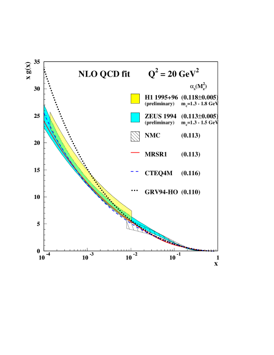
Clearly, the density cannot increase forever; eventually saturation effects will set in [58, 59]. The effective transverse size of a gluon that is probed by a photon of virtuality is . Fluctuations below that scale happen, but cannot be resolved. When such gluons of transverse size fill up the whole transverse area offered by the proton, they will start to overlap and recombine. This would be a novel and very interesting situation indeed: high parton density, but large enough for to be small! Given the size of the proton , the critical condition for saturation effects to turn on can be estimated [59] as . This value is by far not reached by the measured gluon density (Fig. 3.3a). It could be however that saturation does not set in uniformly over the proton’s transverse area, but starts locally in so-called hot spots [60]. In this case would be larger. The inclusive structure function data however do not require any saturation correction. Even a conspiracy of two new effects, a sharp rise of from BFKL evolution dampened by saturation effects, cannot be ruled out. Probably saturation effects will be first seen in hadronic final state data [60].
From an analysis of the scaling violations , or equivalently, from a QCD fit to the data, the strong coupling constant can in principle be determined. From an analysis of the 1993 data was obtained [61]. It is estimated [62] that ultimately, with an integrated HERA luminosity of 500 , can be extracted by a NLO QCD analysis from the HERA structure function data with an experimental error of , and a theoretical uncertainty of . The theoretical errors could be reduced by higher than NLO calculations.
3.3 The Longitudinal Structure Function
One can express the longitudinal structure function in terms of the cross section for the absorption of longitudinally polarized photons (see section 2.1),
| (3.2) |
Longitudinal photons have helicity 0 and can exist only virtually. For transverse photons with helicity the spin is parallel to the direction of propagation, and the field vector perpendicular to it. In the QPM, helicity conservation at the electromagnetic vertex yields the Callan-Gross relation () for scattering on quarks with spin . This does not hold when the quarks acquire transverse momenta from QCD radiation. Instead, QCD yields the Altarelli-Martinelli equation [63]
| (3.3) |
exposing the dependence of on the strong coupling and the gluon density. At small , the second term with the gluon density is the dominant one. In fact is not a bad approximation for [64].
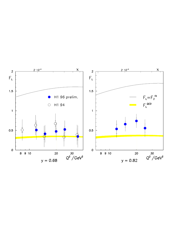
The extraction of from the cross section measurement (eq. 2.1) so far had to make an assumption for , because there existed no direct measurements in the HERA regime. At large , , this is a 10% correction. The argument can be turned around, and can be extracted at large from a measurement of the cross section, assuming that follows a QCD evolution and can be extrapolated from measurements at smaller . This procedure has been carried out by H1 [42, 41] (Fig. 3.4). The extracted excludes the extreme possibilities =and =0 and implies , since . This is self consistent with the gluon density extracted from the H1 QCD fit. It should be noted however that the data points at high are somewhat above the expectation from the QCD fit. More precise measurements are necessary to clarify the situation. A measurement of without theoretical assumptions on the evolution of will be possible by measuring the DIS cross section at HERA at two different centre of mass energies [65], because these data will allow to vary in eq. 2.1 while keeping and fixed.
3.4 and the Transition between DIS and Photoproduction
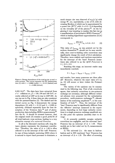
The total cross section is shown as a function of in fig. 3.5. The cross section increases with , and the slope increases with .
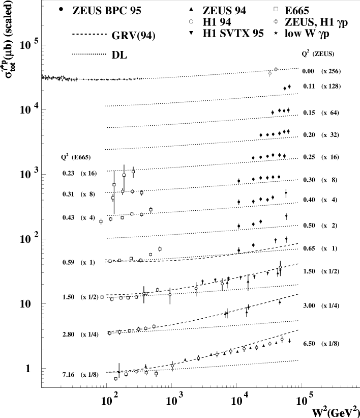
The data at are well described by the soft Pomeron parametrization by Donnachie-Landshoff (DL) [30], . With increasing , the cross section grows faster than the DL prediction. There appears to be a smooth but rather fast transition between the soft and the perturbative regions. Already at , a distinctively fast rise of the total cross section with is observed. The H1 fit result translates into with for .
The perturbative GRV mechanism [49] utilizing NLO DGLAP evolution provides an adequate description of the data down to . It has not been possible to apply NLO DGLAP at lower to describe the data. For example, below the GRV curves would turn over at small , reflecting the valence-like behaviour of the GRV input partons at a low scale, by far failing to account for the data [35].
Chapter 4 Models for Hadron Production in DIS
4.1 Reference Frames
In this section the different reference frames and the variables used to describe the hadronic final state are introduced. Rough expectations for the event properties are derived mainly from phase space arguments. They will be refined by perturbative QCD and specific hadronization models.
The laboratory frame
The HERA experiments are performed in the “laboratory frame”, in which the detector is at rest, and the incoming electron and proton beams are collinear. The axis is defined by the proton beam direction. After the collision, the transverse momentum of the scattered electron is balanced by the one of the hadronic system. The hadronic final state is however better studied in a frame where the transverse boost is removed, such that the virtual photon and the incoming proton are collinear. Photon and proton 4-vectors are denoted by and . With the proton mass can be neglected.
The hadronic CMS
The hadronic centre of mass system (CMS) is defined by the condition . The invariant mass of the hadronic system is given by . The positive -axis is usually defined by the direction of the virtual boson, . All hadronic final state particles with 4-momentum which have are said to belong to the current hemisphere, and all particles with are assigned to the target or proton remnant hemisphere. Target and current systems are back to back and carry energy each. They are not necessarily collinear with the incoming proton. In the QPM however, a quark in the proton with 4-momentum absorbs the virtual photon and is scattered back with 4-momentum . The proton remnant retains the 4-momentum . With these assumptions, the scattered quark and the proton remnant are both collinear with the incoming virtual photon and the proton (fig. 4.1). This is no longer the case if one considers intrinsic transverse momenta of the partons in the proton, or generates transverse momenta perturbatively by radiation.

The Breit frame
The Breit frame (BF) is defined by the conditions that proton and virtual photon are collinear, and that the virtual photon does not transfer energy, just momentum. Since , with the same orientation as in the CMS, and . In the QPM, the incoming quark absorbing the virtual photon does not change its energy, but reverses its longitudinal momentum with magnitude (fig. 4.2). The Breit system is also called the brick wall system, because in this picture the quark bounces back like a tennis ball off a brick wall. Neglecting the quark mass and transverse momenta, its 4-momentum is before and after the scattering. The incoming 3-momentum vector is merely reverted.
Again, all particles with are assigned to the Breit current hemisphere. The CMS and BF are connected via a longitudinal boost. The division into current and target hemisphere is frame dependent. In both systems, the remnant diquark is a mere spectator in the sense that its momentum remains unchanged.

4.2 Kinematics and Variables
Let us consider a particle with 4-momentum and mass , which travels under an angle with respect to the axis. We define the transverse momentum , the transverse mass and the transverse energy .
The rapidity [70] of a particle is defined as
| (4.1) |
The rapidity transforms under a boost in the direction with velocity as
| (4.2) |
Hence the shape of the rapidity distribution is invariant against longitudinal boosts. A useful relation is
| (4.3) |
Often the mass of a measured particle is not known. One therefore defines the pseudorapidity
| (4.4) |
For , .
Energy and momentum of a particle are conveniently scaled by their kinematically allowed maximum, leading to the definitions
| (4.5) |
For and , these definitions converge: . We shall use as a generic symbol for the variables defined in eq. 4.5.
The scaled longitudinal momentum is known as Feynman-. In the CMS, , with . Similarly, in the Breit frame current hemisphere with . None of the variables defined in eq. 4.5 is Lorentz invariant. A Lorentz invariant that is currently not being used at HERA is . In the proton rest frame it gives the fraction of the energy transfer taken by the produced hadron, . For large and the differences between and are small.
The rapidity can take any values with (see fig. 4.3), with
| (4.6) |
In the CMS, . At HERA with , pions can be produced with . Neglecting transverse momenta, the CMS rapidity is related to (for ) by
| (4.7) |
The difference of rapidities measured in the Breit and the CM systems is
| (4.8) |

4.3 Simple Mechanisms for Hadron Production
Much can be learnt about the gross event features already from phase space considerations and a few simple assumptions. We start with the simple model of independent fragmentation, applied to the scatterd quark and the remnant. In the following sections, this naive picture will be refined with perturbative QCD radiation and more sophisticated hadronization models.
The Lorentz invariant cross section for hadron production may be written as
| (4.9) |
since . For a distribution that is isotropic in azimuth , the integration yields
| (4.10) |
We describe the inclusive densities to find a hadron with energy fraction from the fragmentation of a quark with fragmentation functions . ( is not a probability density, because its integral is not 1.) They scale approximately, that is they depend only on the fractional hadron energy and not on the quark energy [71]. The resulting hadron spectrum from quark fragmentation in the reaction is then
| (4.11) |
Here is the total event cross section, the number of produced events, and the number of produced hadrons of type . is the quark density function for flavour in the proton.
In the simple model of independent quark fragmentation [72], a quark with energy fragments into a hadron with energy according to a distribution function , where , see fig. 4.4. The process is iterated with a quark carrying the remaining energy until there is no energy left to produce a hadron. It is assumed that in the fragmentation process only limited transverse momenta are produced, usually parameterized with a falling exponential distribution in with .

The model describes the gross features of fragmentation [72], namely energy independence, and for small a behaviour
| (4.12) |
Since , this gives a uniform number density of hadrons in rapidity, the so-called central (in the CMS) rapidity plateau:
| (4.13) |
Fig. 4.5a gives the relation between the longitudinal momentum for a typical HERA situation. translates roughly to the rapidity region (fig. 4.5a).


A convenient parametrization for the fragmentation functions is
| (4.14) |
Energy-momentum conservation requires
| (4.15) |
where the sum runs over all hadron species . If we do not distinguish between hadron species, we can define . The normalization is then fixed by
| (4.16) |
A useful parametrization for light quarks , accurate to , is [73]
| (4.17) |
see fig. 4.5b. The average number of hadrons per unit rapidity in the plateau region ( small) is then
| (4.18) |
of which roughly 2/3 will be charged. The rapidity plateau is depicted in fig. 4.3. There will be a kinematic fall-off for . The available rapidity range increases logarithmically with the quark energy (longitudinal phase space), and so does the average total hadron multiplicity.
The average total hadron multiplicity in a quark jet is given by
| (4.19) |
where is determined by a typical hadron mass . From
| (4.20) |
we obtain a logarithmic scaling law for the multiplicity
| (4.21) |
where is the integration constant.
Though the independent fragmentation picture describes crudely the data on e.g. , it has its limitations. It cannot be applied consistently for small , , it is not Lorentz invariant (the constants and are frame dependent), and energy momentum conservation has to be enforced by hand after both quarks have fragmented. The lack of Lorentz invariance even leads to contradictions. Let be the total CM energy. In the CMS, one calculates for the total multiplicity with . In a frame where one quark takes almost all of the energy, and the other one only very little, one gets a different value with
The discussion so far covered only the lowest order processes, where hadron production is determined by the assumption of limited transverse momenta and longitudinal phase space as a simple hadronization model. Though simple, it provides a good guideline for hadron production. QCD radiation modifys this simple picture and will be discussed next (section 4.4). Afterwards improved hadronization models are introduced that do not suffer from the problems with the independent fragmentation model (section 4.5).
4.4 Perturbative QCD Radiation
The perturbative part of QCD radiation is treated either with fixed order matrix elements, or with parton showers, or a combination of both. It depends on the application which treatment is most appropriate. In general, the matrix element will become more important with increasing hardness of the interaction. Perturbative QCD makes predictions for partonic final states, but observed are hadronic final states. To make contact with the experimentally accessible world, hadronization has to be taken into account. Models for the non-perturbative effects of hadronization are discussed in section 4.5. Excellent reviews on perturbative QCD evolution and on hadronization are [74, 75]. Further information specific to DIS can be found in [76]. We start the discussion of perturbative QCD with matrix elements and parton showers. An alternative technique which is not based on Feynman diagrams is the dipole radiation approach, to be discussed afterwards.
Matrix elements
In fixed order perturbation theory, the incoming parton flux is folded with the matrix element [77] for electron-parton scattering which leads to some final state parton configuration. In LO possible final state configurations for scattering are (apart from the scattered electron) (QPM), (QCDC), and for electron gluon scattering (BGF) (fig. 4.6). In NLO, one additional parton can be emitted, and so on.


The calculations are ususally done numerically. For state of the art NLO calculations the programs DISENT [78], MEPJET [79] and DISASTER++ [80] are available. Originally such programs could only be used for jet analysis. The present programs are more flexible and allow also calculations of for example event shape variables.
Leading Log parton showers
A complete calculation to an order higher than NLO appears prohibitive. For many applications, where higher orders are important, the parton shower ansatz is used. For example, higher orders can be summed to all orders in the leading log approximation. In the DGLAP (leading ) approximation, they result in splitting functions which give parton emission probabilities.
When a parton with 4-momentum radiates, it changes its virtuality . The evolution parameter increases in the initial state parton shower (space-like shower) by successive emissions, and decreases in the final state parton shower (time-like shower). The probability that a branching will take place during a small change is given by the evolution equation [15]
| (4.22) |
The functions are just the Altarelli-Parisi splitting functions in eq. 2.14, .
Such calculations are usually done with Monte Carlo event generators, where the parton shower evolution is simulated step by step according to the emission probabilites, until the whole event is generated. Perturbative evolution is stopped at some small scale of , when it becomes unsafe to apply perturbation theory due to the growth of .
When combined with the exact fixed order matrix element to take care of very hard emissions that are not properly covered with leading logs, the Monte Carlo event generators can be expected to provide a good representation of what is actually happening in DIS events111 Remembering the double slit experiment, we should feel a bit uneasy about a statement of what is actually happening. (fig. 4.7). Ambiguities result from the way the matrix element and parton shower are combined (“matching”), coherence effects are treated, divergencies of the matrix element are cut-off, and from other approximations in the implementation. Unfortunately todays generators implement the matrix element and parton showers only to LO.
Examples of DIS Monte Carlo generators that are based on leading log DGLAP parton showers are LEPTO [81], HERWIG [82] and RAPGAP [83]. They are expected to be valid where the DGLAP approximation is valid. As DGLAP based models, the initial state parton shower is strongly ordered in , increasing from the proton towards the matrix element.
The leading log approximation (LLA) can also be applied directly for specific observables, without utilizing an event generator. Most relevant is the modified leading log approximation (MLLA) which takes into account destructive interference between soft gluons, in conjunction with the assumption that the resulting parton spectra resemble the observable hadron spectra, up to a constant factor (local parton hadron duality, LPHD).

The colour dipole model
Another type of parton shower model is the colour dipole model (CDM) for QCD radiation [84]. The colour charges of the scattered quark and the remnant are assumed to form a colour dipole, from which gluons can be radiated (fig. 4.8a). Subsequent gluon radiation emanates from dipoles spanned between the newly created colour charges and the others, and so on. To good approximation it can be assumed that these dipoles radiate independently. The CDM uses the LO cross section for the emission of a gluon with transverse momentum at rapidity in the soft gluon approximation [85],
| (4.23) |
The cross section is uniform in rapidity and . Kinematically, the phase space is bounded by , where is the total energy of the radiating system. Gluons with above a certain cut-off, , lie inside the triangle in fig. 4.8b.


In DIS one of the colour charges is not pointlike, the proton remnant. The suppression of radiation with short wavelength from an extended source is taken into account with a special parameter of that describes the extendedness of the remnant remnant222In the recent version also the colour charge of the scattered quark is spread out, depending on the “size” () of the final state quark that can be resolved with the photon of virtuality .. The CDM is implemented in the program ARIADNE [86]. In ARIADNE the QCDC graphs are covered by dipole radiation (and corrected to yield the exact LO matrix element contribution), but for the BGF graph the matrix element is used. Further radiation is then according to the CDM.
In contrast to the LL parton shower in the CDM it is not possible to distinguish between initial and final state radiation, or to reconstruct an “evolution path” for the parton in the proton that is hit by the virtual photon. Kinematically, the phase space for radiation is bounded by the of the previous emission. In rapidity the emission probability is uniform. Therefore the final gluon configuration is not ordered in , if one arranges them according to increasing rapidity (see fig. 4.8b). Rapidity is directly related to for fixed and (see section 8.1). In that respect the CDM is similar to what can be expected from BFKL evolution [87], though perhaps in a somewhat unconventional fashion [88]. Whereas the LL parton showers are connected with the intuitive picture of an evolution path, it is probably fair to say that the significance of the dipole model is not yet understood very well. We shall see that this model provides effortlessly overall the best description of most final state data. This is probably the main reason why it is being discussed, whether or not it has a deeper physical justification not yet appreciated by the community.
The Linked Dipole Chain Model - LDC
The CCFM approach for the hadronic final state has been reformulated in a picture similar to the CDM, giving rise to the Linked Dipole Chain model (LDC) [24]. This model is particularly interesting, as it should converge to the DGLAP and BFKL predictions in their respective regions of validity, and handle properly cancellations between real and virtual emissions for the final state. In the LDC also the case is treated where the largest of the process is not attached to the virtual photon vertex. Some promising results from a Monte Carlo implementation of the LDC have been obtained [89], but the program is not yet publicly available.
Coherence
Quantum mechanical interference is an important issue for the hadronic final state. With matrix elements that sum and square amplitudes interference effects are taken into account naturally. Coherence effects in parton showers that rely on emission probabilities, not amplitudes, require special attention. One may distinguish a) interference between initial and final state radiation; and b) interference between partons emitted either in the initial state or in the final state parton shower.
In the CDM there is no distinction between initial and final state radiation, so in the dipole approximation problem a) does not arise. Also soft gluon interference is automatically taken into account by the dipole mechanism. In other generators such interference effects can be realized by phase space restrictions for parton emission. For example, the effect of destructive interference between subsequent emissions in a parton shower can be approximated by imposing a posteriori “angular ordering”: only emissions are allowed with a smaller opening angle than the previous one, .
The physical reason for this condition is that large wavelength quanta cannot be emitted from dipole sources with small transverse dimensions. This can be seen easily for cascades [90]. Consider the example fig. 4.9a, where a virtual photon branches into an pair, and the radiates a photon. The formation time of the final state can be estimated as the lifetime of the intermediate from its off-shellness , . We have , and for small angles, Since for soft photons, , . During this time the pair have separated a transverse distance . The transverse wavelength of the emitted photon is with . If is larger than , the photon cannot resolve the individual charge of the , it rather sees the combined charge of the pair, which is 0. For allowed emissions it follows , or , angular ordering.
In QCD the situation is a bit more complicated, because the incoming parton is colour charged (fig. 4.9b). Parton cannot be radiated incoherently from parton when . In that case it would see the combined colour charge of and , which is the colour charge of the incoming parton . Parton with can therefore be treated as effectively being radiated from before branches off, thus restoring angular ordering.


4.5 Hadronization
Experimentalists follow two different philosophies how to prepare their hadronic final state data.
-
•
In one approach, the data are corrected just for detector effects in order to remove any experimental bias and be able to compare the data to other experiments. The data are corrected “to the hadron level”, they represent a measurement of observable hadrons. The data can also be compared to QCD predictions that include hadronization effects, but not directly to perturbative QCD calculations (unless one is interested to study the difference between observable hadrons and partonic calculations).
-
•
In the other approach, a hadronization model is used to correct the data for hadronization effects back “to the parton level”. The data can then be compared directly to perturbative QCD calculations. A problem of principle arises: partons are not observable, so strictly speaking an observable “at the parton level” does not exist. With great care one may proceed nevertheless. One has to specify the parton level in perturbative QCD (like NLO, LLA, including cut-offs etc.), and correct the data for all other effects beyond that: higher order corrections plus hadronization effects. The observable thus becomes scheme dependent. There is another price to pay: the data have picked up a theoretical bias due to the assumptions on higher order and hadronization effects. In practice this bias is studied by comparing different Monte Carlo generators. The encountered differences are treated as systematic error of the measurement.
We summarize the main approaches to hadronization, some of which have already been mentioned. It has to be emphasized that the boundary between perturbative QCD evolution and hadronization is not uniquely defined. Ideally, predictions for final state observables would not depend on how the boundary is defined, for example on the lower cut-off for virtualities in the parton shower.
We start with hadronization models that are implemented in Monte Carlo generators (independent fragmentation, string and cluster model). Other approaches that model only specific aspects of hadron production are discussed afterwards.
Independent fragmentation [72]
From the fragmenting parton mesons are produced, carrying a certain fraction of the original energy, see section 4.3 and fig. 4.4. The branching is repeated with the remaining energy until all the energy is used up. In the physical picture for independent quark fragmentation the quark forms a meson with an antiquark from a pair, with the remaining quark continuing fragmentation. It is assumed that the distribution of is energy independent, leading to scaling fragmentation functions. Furthermore, all partons of an event fragment independently. That leads to inconsistencies like non-conservation of energy-momentum, that have to be cured by hand.
Transverse momentum components are assumed to be Gaussian distributed333 The transverse momentum which a primary hadron receives from the fragmentation process can be described by Gaussians in and with widths , (4.24) This leads to an exponentially falling distribution in with , (4.25) It follows, that the distribution in is neither Gaussian nor exponential, (4.26) with . The default parameter in the Monte Carlo program JETSET [91] is . [92], which results in an exponentially falling distribution in . From the parametrizations used in fragmentation models [92, 91], is obtained for primary hadrons.
String fragmentation [93]
In the Lund string model, a quark and an antiquark moving apart stretch a colour field between them. The field is thought to be string-like with constant energy density per unit length of , and with transverse dimension of . When the stored energy becomes large enough, the string can break up and create a pair from the vacuum (fig. 4.10a). The newly created and terminate the loose string ends, such that the new string pieces are themselves colour neutral. The process is iterated with the new strings until all the available energy is used up. Transverse momentum components result from a tunneling process; they are parametrized as in eq. 4.24. The string model gives rise to scaling fragmentation functions, a rapidity plateau with uniform particle density, and a logarithmic increase of particle multiplicity , where is the string invariant mass.

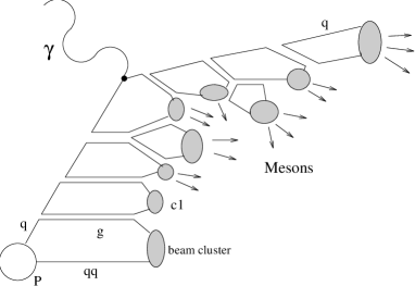
String fragmentation can be formulated in a covariant way, it does not suffer from the mentioned shortcomings of independent fragmentation. Furthermore, some quantum mechanical interference effects in gluon radiation are taken into account with string fragmentation, due to the way gluons are treated. Carrying two colour charges, gluons are always the endpoints of two strings. In a configuration the gluon is realized as a kink in the colour connection between the pair. Destructive gluon interference leads to a suppression of radiation (and finally hadron production) in the region opposite to the gluon. Because in the string model there is no string spanned directly between the and the this “string effect” [94] appears naturally in the Lund model.
Cluster fragmentation [95]
According to the idea of “preconfinement” [96], colour connected partons tend to be close in phase space towards the end of the perturbative phase. This property is exploited in the cluster fragmentation model. After the perturbative evolution all gluons are forced to split into pairs. Colour connected pairs are combined into low mass colour neutral clusters, which decay into mesons according to phase space (fig. 4.10). Due to the small cluster mass, relatively few parameters are needed to describe the cluster decay. Nevertheless, large mass clusters may occur; they are split longitudinally in a fashion similar to the string model before they are allowed to decay.
Local Parton Hadron Duality (LPHD)
The hypothesis of local parton-hadron duality (LPHD) [97] is made to allow predictions for hadron spectra from perturbatively calculated parton spectra. It states that any hadron cross section depending on a quantity is related to the corresponding partonic cross section simply by a constant factor, . The idea behind this seemingly surprising ansatz is that if perturbative evolution is used for multi-parton emissions down to a very low scale, there is not much energy left for hadronization to change the shape of the distribution. This hypothesis could be applied successfully to a variety of phenomena, but one should keep its limitations in mind [98]. For example, when a quark and antiquark separate and do not radiate any gluons (unlikely, but possible), LPHD would predict a gap in rapidity in between, devoid of any hadrons. A more physical assumption is that the colour field stretched between quark and antiquark leads to the production of hadrons filling the gap. At HERA, the LPHD hypothesis has been applied to charged particle spectra, see sections 5.2 and 6.1.
Fragmentation functions
The number density to find a hadron with energy fraction from the fragmentation of a quark is described by a fragmentation function , and similarly for a gluon . They scale approximately, that is they depend only on the fractional hadron energy and not on the quark energy [71]. QCD effects like gluon radiation off the quark make the fragmentation functions scale dependent: , where the scale is provided by the hard process (fig.4.11). While the fragmentation functions themselves are not calculable in perturbative QCD, their scale dependence can be calculated in the same way as the scaling violations of the structure functions in DIS [99].

The fragmentation functions obey an evolution equation
| (4.27) |
is the factorization scale between the parton production process and the parton fragmentation process. The splitting functions for branchings are in leading order the same as for the parton densities in DIS, eq. 2.14, but differ in higher order [99]. They have been calculated up to next-to-leading order [100].
The fragmentation functions are universal, that is process independent. For example, quark fragmentation functions measured in can be used to predict the hadron distribution in the quark jet for .
High energy and power corrections
Due to the limited generated in hadronization, it appears plausible that with increasing energy the relative importance of hadronization effects diminishes for suitably chosen observables. It is expected that for infrared safe quantities (see section 2.6) like jet observables and some event shape variables their perturbative prediction approaches the value that is observable with hadrons. The difference, due to higher orders and hadronization, should decrease like an inverse power of the energy , a “power correction” [101]. Power corrections have been investigated for thrust and other event shape variables at HERA, see section 6.2.
4.6 Rapidity Gaps
At HERA there exists a class of events known as “rapidity gap events” [102, 103, 104, 105]. They have given rise to tremendous activity, which would deserve a review in its own right (recent summaries are [3]). Here as much is covered as is relevant for our purpose.
Rapidity gap events exhibit a sizeable region of rapidity without any hadronic activity – the rapidity gap, see fig. 4.12. In normal events a colour field forms between the scattered quark and the proton remnant, leading to a homogeneous distribution of hadrons populating the available rapidity range. Large gap sizes between neighbouring hadrons from normal fragmentation are expected to be unlikely (though possible). Large gaps can be produced however in processes where two systems are produced that are not colour connected.


Events with large rapidity gaps had been anticipated for HERA from processes with Pomeron exchange [107], though the large rate came as a surprise: about 10% of all DIS events have a large rapidity gap444Often these events are called “diffractive”, or being due to a diffractive process. The meaning of these terms is not yet uniquely defined amongst the experiments and theorists. We therefore prefer the term “large rapidity gap”, because the existence of a gap of a certain size is well defined event by event.. In the Ingelman-Schlein model [108] a Pomeron is exchanged in the channel between the proton and the virtual photon, see fig. 4.13a. The proton may be left intact, or fragment into a low mass system . In the Ingelman-Schlein model, the virtual photon interacts with a parton in the Pomeron, thus probing the structure of the exchanged Pomeron. The resulting system with mass is not colour connected with the proton remnant system, because the Pomeron carries no colour. A rapidity gap between the two systems is the consequence.


Suppose the above picture to be valid, the partonic structure of the elusive Pomeron can be probed! In fact, the evaluation of the rate of rapidity gap events suggests that the exchanged object is predominantly gluonic, and that most of the Pomeron momentum is carried by one single gluon [3]. The analyses suggest furthermore that the Pomeron intercept in DIS is somewhat larger than expected from the soft Pomeron, and possibly increasing with [3].
Other models assume that rapidity gaps are due to changes in the colour structure of the event after the hard interaction has taken place [109, 110]. At low , most events are due to photon-gluon fusion, resulting in a colour octet - antioctet configuration in the final state. In the string model, there would be two fragmenting strings spanned (fig. 4.14a). It is assumed that while the produced quark and antiquark travel to leave the proton, soft gluons are exchanged between them and the proton remnant, see fig. 4.13b. These gluons do not change the momenta significantly, but may rotate the colour configuration of the quark - antiquark pair. The final configuration may turn out to be a colour singlet, in which case there would be no colour field connecting it with the remnant (fig. 4.14c). The attractive feature of this model is an explanation of the absolute rate of rapidity gap events. If soft gluon exchange results in a random colour configuration, the ratio of colour singlet to colour octet configurations would be , and ! In a related semiclassical approach, partonic fluctuations of the virtual photon are scattered by the colour field of the proton [111].
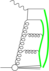
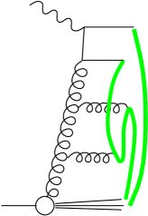
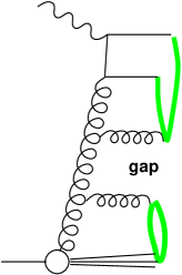
Both models describe at least qualitatively the HERA data on rapidity gap events. Detailed studies will be necessary to discriminate them (for example in the final state of the system [112]), or perhaps discover them to be not exclusive at all555Pomeron exchange where most of the momentum is carried by one gluon in the Pomeron is not so much different from boson-gluon fusion, where the hard dynamics is determined by the incoming gluon, and soft gluons are only needed for colour neutralization. For the discussion of the hadronic final state in DIS it will be important to keep the existence of rapidity gap events and possible production mechanisms for them in mind. Some analyses [113, 114, 115, 116, 117, 118] explicitly exclude rapidity gap events, others don’t, and some study the difference between the two samples. The possible existence of a mechanism to change the colour configuration will have a bearing on the interpretation of certain final state data at small (section 8.1). Colour reconnections are also being discussed in connection with fragmentation at LEP [119, 120].
4.7 Monte Carlo Generators
We shortly summarize the DIS Monte Carlo generators. They incorporate the QCD evolution in different approximations and utilize phenomenological models for the non-perturbative hadronization phase. The events are generated according to the electroweak cross section with experimentally determined input parton densities. QED radiative effects are treated with special programs [121, 122].
The Monte Carlo results depend on the model parameters, which can be adjusted to the data. Information on generator tuning can be found in [123, 124, 125, 76]. In general, the generators now give an overall satisfactory description of the data. None of the generators however is able to describe all aspects of the data.
LEPTO
LEPTO [81] is based on the LO QCD matrix element with leading log DGLAP parton showers for soft emissions. Therefore the model is often called MEPS (Matrix Elements + Parton Showers). Angular ordering is imposed to model colour coherence. The rather sophisticated Lund string model [93] as implemented in JETSET [91] is used for hadronization. A special feature are “soft colour interactions” (SCI) [109] in the hadronization phase. They lead to string rearrangements. This feature is now default, because it describes at least qualitatively events with a large “rapidity gap” that are seen in the data.
RAPGAP
Originally, RAPGAP [83] was created for rapidity gap events. They are described by scattering on a colour neutral object, the Pomeron, which is emitted from the proton according to a flux factor, and whose internal structure is described by parton density functions. The present version includes also normal DIS event generation, very similar to LEPTO. In the latest version it is also possible to simulate a resolved (not point-like) component of the virtual photon.
HERWIG
HERWIG [82] is based on LL parton showers, with additional corrections to describe properly the hard interaction. Final state radiation is angular ordered, initial state radiation is ordered in , where and are energy and angle of the radiated parton. The HERWIG philosophy is to model the perturbative phase as accurately as possible, and to hadronize with a relatively simple cluster fragmentation model [95]. Though there is no mechanism foreseen for rapidity gap events, it turns out that they are generated at a surprisingly large rate. Also with HERWIG a resolved component of the virtual photon can be simulated.
ARIADNE
In ARIADNE [86] perturbative QCD radiation is modelled with radiating colour dipoles according to the CDM. The BGF graph is added by hand with its LO matrix element. Hadronization is performed with the string model as implemented in JETSET. ARIADNE allows to model rapidity gaps either by scattering on a Pomeron, or by colour reconnections, but these options are by default not activated666It was found that colour reconnections in combination with the colour dipole model do not give a good description of rapidity gap events at HERA [126]..
Chapter 5 General Event Properties
5.1 Energy Flow
The first analysis of the hadronic final state in DIS at HERA was based on 88 events recorded in 1992 [127]. The measured energy flows and particle spectra were in rough agreement with what was expected from some models including QCD radiation and fragmentation, and exluded certain other radiation scenarios.
The flow of transverse energy as a function of pseudorapidity provides a very simple, global characterization of the hadronic final state. It is measured with the calorimeters and includes all produced particles, except the scattered electron. The flow as a function of pseudorapidity is defined as
| (5.1) |
where the sum extends over all particle species with cross sections . The definition is analogous for the flow as a function of azimuth . The distribution is normalized to the total number of events , corresponding to the total event cross section .
It is instructive to examine the flow of hadronic transverse energy as seen in the HERA detectors in the laboratory frame, fig. 5.1. In this frame one measures according to eq. 5.1 the energy flow transverse to the beam line as a function of pseudorapidity and azimuth . Here is the angle with respect to the proton beam axis (laboratory ), and is the angle between the energy deposition and the scattered electron in the plane transverse to the beam line. One sees the current jet from the scattered quark emerging opposite to the scattered electron in (fig. 5.1 right). The rapidity region from the current jet towards the remnant is filled with particles due to the colour field stretched between the scattered quark and the remnant (the main calorimeter acceptance ends at typically ), see fig. 5.1 left.


Significantly more transverse energy is observed between the current jet and the beam pipe than is expected from the QPM without QCD radiation, but including fragmentation. The QPM predicts an of roughly 1 GeV per unit pseudorapidity; one arrives at a similar number from the simple considerations in section 4.3, assuming 3.5 hadrons per unit rapidity with an average of 0.35 GeV . The extra can be attributed to hard and soft gluon radiation. The models for these processes varied a lot in their predictions, but have evolved since.
In fig. 5.2 the latest preliminary H1 data on energy flows in the hadronic CMS [115] are compared to the model LEPTO 6.4 with different treatments for perturbative QCD radiation. Without QCD radiation, a flat rapidity plateau with per unit rapidity is expected. QCD radiation as expected from the hard matrix element generates in the current hemipshere only. It is shown below that the in the current hemisphere depends on . With parton showers only, a reasonable description of the data is achieved. For this observable, the parton shower covers already most of the relevant phase space, including the matrix element. The best description of the data is obtained by combining radiation according to the LO matrix element with parton showers.

The energy flow has also been studied as a function of (fig. 5.3). At low the rapidity plateau is almost flat. With increasing , the in the “photon fragmentation region” (loosely defined as far in the current hemisphere) increases considerably. In that region, the virtuality of the photon governing hard interactions plays an important rôle. At central rapidity, the dependence is comparatively small. This supports qualitatively the picture that particle production at central rapidity is independent of the type of the colliding particles, be they or a virtual photon [129].

5.2 Charged Particle Multiplicities
Average multiplicity
The multiplicity of charged particles in the CMS current hemisphere () has been measured by H1 [116] with their central tracking chamber for events111Rapidity gap events had been excluded from this analysis. at in the kinematic range (fig. 5.4a), thus reaching fragmentation energies not yet accessible at LEP. From phase space arguments alone, one would expect , (see section 4.3). Scale breaking due to QCD radiation should lead to a faster rise of the multiplicity, however dampened by colour coherence and the running of . A faster than logarithmic rise is observed when comparing the H1 data to lower lepton-nucleon scattering experiments. The QCD model LEPTO somewhat overestimates the multiplicity (see fig. 5.4). The DIS data are also compared to the JETSET prediction (light quarks only) for data, which is known to give a good representation of the data. The behaviour of the total multiplicity in the CMS current hemisphere in DIS is similar to annihilation data. Differences are found however for the distribution in rapidity, see below.

The growth of multiplicity with energy has been calculated via the QCD evolution of fragmentation functions for running in NLO [99, 131], yielding
| (5.2) |
The two-loop expression eq. 2.8 for is used with as scale. The constants and are given by the theory as
| (5.3) |
with active flavours and . and are free parameters.
Predictions for hadron spectra can also be derived from the parton multiplicity in a jet, which is calculable in QCD by summing up all the branchings in the cascade down to a cut-off . The hypothesis of local parton-hadron duality (LPHD) (see sect. 4.5) is made for the transition from partons to hadrons: the hadron spectra should have the same shape as the perturbative prediction, merely differ by a normalization constant. The prediction will depend on the cutoff , because the charged particle multiplicity is not an infrared safe observable, see section 2.6. If one assumes that the shower stops at a scale given by a typical hadron mass , the dependence is eliminated. One can then compare the perturbative prediction directly to the data.
Most important for the average multiplicity is the growth at small fractional momentum due to soft gluon radiation. Quantum mechanical interference leads to a suppression of soft gluon radiation (soft colour coherence). The shower evolution in the leading-log approximation (LLA) is modified (hence called MLLA) to take into account destructive interference of soft gluons [90]. The modification consists of changing the evolution variable such that angular ordering [90, 132] between subsequent emissions and is fulfilled. That is, their opening angles satisfy (see section 4.4).
The MLLA+LPHD prediction for the hadron multiplicity for running is [90, 98]
| (5.4) |
with
| (5.5) |
where , , and . is the Gamma function and the modified Bessel function of order . is used [98]. Eq. 5.4 reduces to eq. 5.2 for large .
The data can be fit by either eq. 5.4 or eq. 5.2. For fixed one would expect a faster growth than eq. 5.4, namely a power law [98]
| (5.6) |
which is still consistent with the data. In fact, all these fits would be indistinguishable in fig. 5.4. The fit with eq. 5.2 yields and . In this fit the correction term has been neglected, because it had been found insignificant (). It has to be pointed out that extracted from eq. 5.2 need not be identical with , though they are expected to be similar if is small [131]. The fit results are summarized in table 5.1.
Multiplicity Distributions
H1 has also measured the multiplicity distribution , giving the probability to observe in a given event charged particles, as a function of , and for varying pseudorapidity ranges. In general, the data can be parametrized with the Negative Binomial Distribution (NBD),
| (5.7) |
The two parameters can be expressed in terms of the average multiplicity and the dispersion :
| (5.8) |
One arrives at the NBD in many phenomenological models [133] for hadron production. A large body of data can be parametrized by the NBD. In QCD the LLA also leads to the NBD for the gluon multiplicity in a quark jet [134]. An alternative function is the Lognormal Distribution (LND), derived for multiplicative branching processes [135]. A variable is distributed according to the LND, if its logarithm is Gaussian distributed. The H1 data (fig 5.5) are equally well described by both parametrizations. The MEPS model deviates from the data both for very small and large multiplicities. In particular the origin of the excess of 0-prong events in the data over the MEPS model is not clear. For fixed , a dependence of or in the range was not found, within errors.

Hard gluon radiation would lead to a superposition of different NBDs, hence deviations from a single NBD for the hadron multiplicity distribution. A multi-jet induced shoulder structure as observed at LEP [136] is however not visible in the H1 data.
In fig. 5.6 the multiplicity distribution is plotted in the scaling KNO (Koba, Nielsen and Olesen) form [137], as a function of . In a broad class of production mechanisms, based upon scale invariant stochastic branching processes, is expected to depend only on , and not on energy [138]. The H1 data for pseudorapidity for different bins exhibit KNO scaling, and agree with the JETSET result for annihilation.

In fig. 5.4b and c the energy dependence for the ratio and the normalized second order factorial moment [139] are shown (further data on the moments of the multiplicity distribution can be found in [116]). For strict KNO scaling, they should be energy independent, which is the case for HERA energies at large , but not for data at smaller . The data are rather well reproduced by the JETSET model, and by the MEPS DIS model. A QCD calculation approaches the measurements when NLO corrections are taken into account [140], but deviates still significantly from the data. The LO result in the double logarithmic approximation (DLA), , is reduced in NLO[140] to , where . Missing higher order effects, which are taken into account with parton showers in MEPS, may be responsible for the disagreement.
Rapidity Distribution
H1 has measured the charged multiplicity as a function of pseudorapidity [118] for different kinematic regions at low , see fig. 5.7. In the plateau region about 2.5 charged particles per unit are observed. The QCD models describe roughly the data, but are far from perfect. In particular HERWIG overshoots the data at low towards the central region. We mention already here that quite substantial differences between the models and the data emerge at small when only hard particles () are considered (between 0.2 and 0.3 such particles are found per unit). This effect will be discussed in detail in connection with low physics in section 8.3.

The charged particle density measured by H1 [116] close to the central region , per unit, is consistent with data from hadron-hadron interactions, see fig. 5.8. When compared with other DIS experiments, a clear increase of the particle density with is seen. The increase of the total multiplicity with is not entirely due to the increasing longitudinal phase space (rapidity), but also due to an increase of the number of particles per unit rapidity, i.e. the height of the rapidity plateau increases with . The average at central rapidity (see section 8.2) in DIS and in hadron-hadron collisions increases with a similar slope (fig. 5.8)
The particle density at HERA is significantly lower than for data, represented by the JETSET result. Also the dependence in is steeper than in hadron-hadron interactions. The DIS data appear to behave as one would expect from hadron-hadron data. That is also true for the transverse energy (see section 5.1) measured at central rapidity [130], see fig. 5.8.
Why are there for the same CM energy less charged particles in DIS than in at central rapidity? A possible explanation is the “antenna effect” [141], that leads to suppressed radiation from the smeared out colour charge of the proton remnant. Another possible explanation is that scaling violations leading to larger multiplicities are stronger in interactions than in reactions due to the larger scale, . The spectra in the CMS and their scaling violations are presented in the next section.

5.3 Charged Particle Momentum Spectra
In this section inclusive charged particle spectra measured by H1 and ZEUS [113, 148] with their central tracking chambers [113, 148] are presented. This limits the acceptance to the CMS current region, . Measured are longitudinal and transverse momentum spectra with respect to the virtual photon direction (fig. 5.9). The kinematic region covered is and for H1, and and for ZEUS.

spectra in the CMS
The Feynman- () spectra are steeply falling with , in fact more steeply than what would be expected from the naive QPM, that is quark fragmentation without QCD radiation (fig.5.10a). The data can be described when QCD radiation is taken into account. Due to gluon radiation, more than one parton share the available energy for fragmentation; therefore less fast particles are produced, and the multiplicity of soft particles increases (fig. 4.11).

The spectra can in principle depend on the available phase space, determined by , and on the virtuality . A dependence on is implied and important, because the parton composition of the proton changes with . The following table 5.2 gives the scales involved.
| (GeV) | () | (GeV) | ||
|---|---|---|---|---|
| LEP () | 91 | 8300 | 91 | – |
| HERA | 120 | 28 | 300 | |
| fixed target (EMC/E665) | 14/18 | 10 | 24/30 |
The DIS spectra measured at HERA [113, 148] are softer than the spectra measured at lower energy fixed target experiments by EMC [149] and E665 [150], see fig. 5.11b. From this comparison it is however not clear whether the difference is due to the different values of , or .

In fig. 5.11a the HERA data are compared with LEP data from DELPHI [151] (divided by 2 to account for the two hemispheres) at similar, though somewhat smaller centre of mass energy . For fragmentation univerality appears to hold, since the HERA and LEP spectra agree. At smaller , the multiplicity is smaller in DIS than in interactions. (The different energy dependence of multiplicities at central rapidity in DIS and is discussed in section 5.2, see fig. 5.8.) The following circumstances may be held responsible for the difference: 1) mass effects due to the different flavour compositions; 2) the BGF contribution to DIS, which is absent in interactions; 3) the scale , which is smaller at HERA than at LEP; 4) the antenna effect due to the extended colour charge of the proton remnant (though is already 2 units of rapidity away from the target region ). Further studies are needed to identify the reason(s) for the difference.
A recent analysis by E665 [152] of the and dependence of the spectra in the range and reveals that at low they depend mainly on , and at large mainly on . The increase with at small is essentially due to the increase of longitudinal phase space. The decrease at large has been attributed to the scale dependence of the fragmentation function.
QCD predictions with fragmentation functions
The hadron production cross section (see fig. 5.12) can be written as a convolution of the parton production cross section with the fragmentation function , which gives the number density to observe a hadron with momentum fraction from the fragmentation of parton . The parton production cross section itself is a convolution of the parton density function for parton species in the proton with momentum fraction , with the hard scattering cross section to produce parton from electron scattering on that parton , . Finally, the cross sections need to be summed over all parton species :
| (5.9) |
The parton densities and the fragmentation functions depend upon their respective factorization scales, and . The hard scattering cross section depends in addition upon the renormalization scale and . The scales are in principle arbitrary; here they are taken to be (not !), the physical scale related with the hard scattering in DIS [153]. The situation in DIS with is different to , where .


With experimentally determined parton densities and fragmentation function parametrizations from other, mainly , reactions [154], the NLO QCD calculation for the HERA spectrum is quite satisfactory (fig. 5.13) [153]. The LO calculation predicts a spectrum that is too hard compared with the data. When moving out of the current fragmentation region, i.e. towards small and negative , these calculations are expected to break down due to fragmentation effects that are not related to the scattered parton.
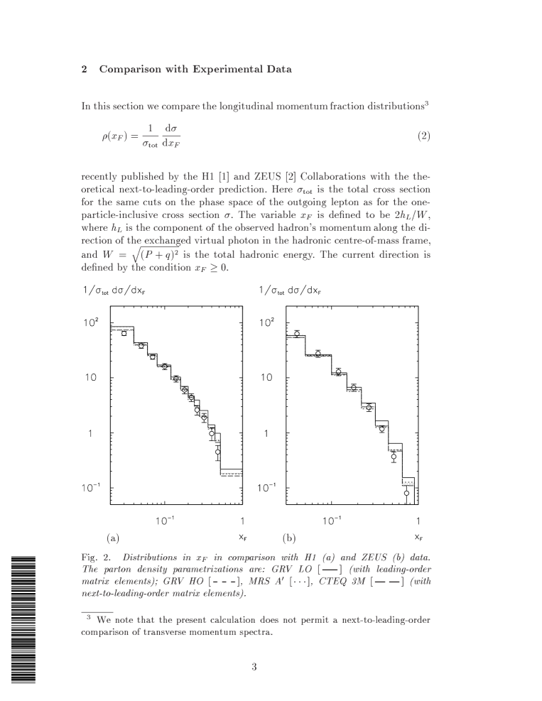
Since the scaling violation of the parton density and fragmentation functions as well as the hard cross section depend on , a measurement of the scale dependence of allows in principle a measurement of . Due to the range covered at HERA, it would be possible to measure from the scaling violations of the fragmentation functions in a single experiment. For an integrated luminosity of 250 a competitive statistical error for of is expected. The theoretical uncertainties are presently estimated to be much larger [153]: from the parton densities and from the scale uncertainty. A better knowledge of parton densities would reduce the corresponding error. Possibly the theoretical situation is more favourable in the Breit system, where the scale of the hard interaction also sets the energy of the fragmenting quark, , similar as in . First indications of scaling violations in the Breit frame are presented in section 6.1.
Transverse momenta
The transverse momentum spectrum of charged particles from ZEUS with is shown in fig. 5.10b. The data exhibit a high tail over the expectation from the QPM without QCD radiation, which is well described by the QCD models. can be generated in the QCD cascade, where partons are emitted before and after the hard scattering. Somewhat arbitrarily one may distinguish radiation from the hard matrix element (BGF and QCDC) and soft gluon radiation (parton shower).
In general, contributions to the of primary hadrons are expected also from other sources than QCD radiation () [155, 5]: from an intrinsic of the initial parton in the proton (), and from fragmentation (). These contributions can be summed up222 An intrinsic of a parton in the proton leads to a tilt of the fragmentation axis with respect to the axis. A daughter hadron with momentum fraction will therefore inherit a transverse momentum . Models assume a Gaussian distribution as in eq. 4.24 with [81] in accord with the uncertainty principle applied to a parton confined to the proton volume. The experimental value is [149]. from fragmentation is also assumed to be Gaussian distributed (eq. 4.24) [92]. A good choice for the description of the HERA and LEP data with the Lund string model is [81, 156, 123]. has been measured with fixed target data [149]. ,
| (5.10) |
The of the finally observed hadrons will be diluted due to decays of the primary hadrons. At HERA, the relative importance of is bigger than at the lower energy DIS experiments. This is best studied in the so-called seagull plot.
In the seagull plot the mean of charged hadrons is plotted as a function of . The data from EMC [149], H1 [113] and ZEUS [148] are shown in figs. 5.14 and 5.10c. The shape of this distribution is reminiscent of a seagull in the sky333 The dip at =0 is mainly a phase space effect. Consider massless hadrons distributed according to the longitudinal phase space model, (5.11) Because , we have (5.12) For small longitudinal momentum, . So for , the cross section is weighted with a factor that grows with for small , giving a large weight to small hadrons in the average . . Due to the limited acceptance to , at HERA only one wing of the seagull plot is measured.

The HERA data are well described by QCD models. Without QCD radiation (the QPM) the prediction falls far below the data. While the QPM predictions are quite similar for EMC and HERA energies, QCD radiation effects are much larger at the higher energy experiments. The increases with [148].
The fixed target data also cover the target fragmentation region, . In the target region QCD radiation is suppressed as compared to the current region. This suppression can be explained with the smeared out colour charge in the proton remnant, if one considers radiation from a colour dipole. Perturbative QCD evolution as implemented in LEPTO yields a similar asymmetry. The description of the EMC data by the CDM (ARIADNE 4.08) is certainly not satisfactory. It would be interesting to try to tune the QCD models to both data samples simultaneously.
At HERA energies an increase of with is observed at fixed , whereas at the lower energy fixed target data from EMC [149] almost no dependence was found, see fig. 5.16. With very precise data in the kinematic region , and the experiment E665 has recently seen a as well as a dependence for the mean [152].
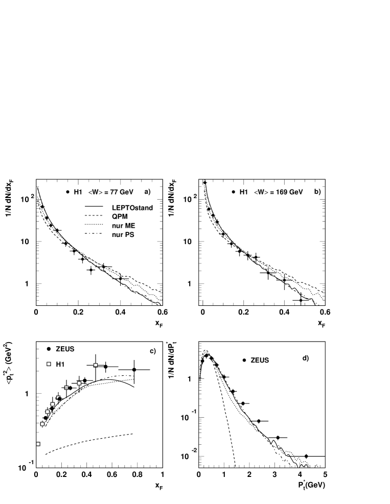
We can use a QCD model to investigate the different contributions to the softening of the spectrum and to the increasing . In the MEPS model (LEPTO 6.4) radiation from the LO matrix element at the photon vertex (BGF and QCDC) can be identified as the main cause; additional soft gluon radiation is relatively unimportant (fig.5.15). On the other hand, the QCD parton shower as implemented in LEPTO appears to cover already a large part of the LO matrix element contribution. Note that the parton shower changes when the matrix element cut-off changes (or is switched off) in order to cover the maximal phase space without double counting (this adjustment is sometimes called “matching”).

5.4 Strangeness Production
Strange particles may be produced in DIS when the scattered quark is a strange quark (either from the sea, or produced in BGF events), of from pairs created during parton showering and hadronization, from heavy quark decays, or from non-standard processes like instantons. Strange particles produced directly from the scattered quark are expected to carry a relatively large fraction of the scattered quark’s energy, whereas most of the strange particles are expected from hadronization with small fractional energy. In the Lund hadronization model, pairs are created in the colour field of the string from the vacuum. Because , pair creation is suppressed with respect to the other light quarks with a ratio . Typically, , with 0.3 the Lund default value representing the experimental mean from [159].
H1 [117] and ZEUS [160] identify and reconstruct and particles via the invariant mass of their decay products in the decays , , . In the following, the notations and include both particles and antiparticles. The decays are measured in the central drift chambers. This limits the acceptance for strange particles in the laboratory system to and . The results for and yields are given in table 5.3. Neglecting the slightly different kinematic selections and averaging the ZEUS and H1 results, for and the yield is per event and unit of pseudorapidity, and for baryons it is .
| H1 | ZEUS | |
| event selection | no large rapidity gap | |
| strange | ||
| particle selection | ||
| # /event | ||
| #/ # charged ∗ | ||
| # event |
The strange particle yield has been studied as a function of , , , , and . In general, the same features are observed as for charged particles. These are an almost flat distribution in pseudorapidity, steeply falling spectra, and no significant dependences on the event kinematics other than on . The ratio of to charged particle yield was found to be the same in events with and without a large rapidity gap, within errors. The average multiplicity in the CMS current hemisphere increases logarithmically with , see fig. 5.17. This behaviour is similar to what has been seen for charged particles, though a faster than logarithmic rise is not seen with mesons (compare 5.2).

The data can be reasonably well described by standard QCD models invoking Lund string fragmentation, provided is chosen. As an example, the spectrum and the seagull plot for mesons are shown in fig. 5.18. The larger observed when going from fixed target to HERA energies can be understood with QCD radiation in the same manner as for charged particles. About the same are observed for s and for charged particles. It is not yet clear why the supposedly scaling spectra of the fixed target data lie below the HERA data for , but this is also expected from Monte Carlo [163]. Probably mass effects play a rôle at smaller energies, in contrast to the HERA data. The H1 data agree with the expectation for annihilation to light quarks at the same CM energy, represented by the JETSET generator.


5.5 Charm Production
The charm yield
Charm production in DIS has been investigated by detecting [166, 167] and decays (and their charge conjugates). The decay products are detected in the central drift chambers. mesons are reconstructed by the invariant masses. mesons are identified by the kinematically tightly constrained mass difference between a candidate and the slow pion, and the candidate mass.
Apart from possible anomalous sources of charm (new particles, instantons, …), the main interest in charm production stems from its sensitivity to the gluon content of the proton at small fractional momentum . The two lowest order standard charm production processes in DIS are boson gluon fusion (BGF) and scattering off a charm sea quark in the proton (QPM)444The boundary between QPM and BGF is subject to definition., see fig. 5.19. At high also an intrinsic (valence) charm component to the proton at the few permil level has been discussed [168]. At small the BGF contribution is expected to dominate due to the increasing gluon content. When the invariant mass of the system is large enough () so that mass effects can be neglected, the quark flavours are expected to be produced according to due to their electric charges, provided one is below the threshold. production is suppressed by the large bottom mass. It has been estimated [169] that in DIS production is , integrated over a large range in , but can be as large as 0.1 at small and large , that is large . There are no results on open production from HERA yet.


The charm cross section555The elastic (diffractive) cross section for is comparably small, pb for and [170]. is inferred from the production rate by taking into account the charm fragmentation function and the appropriate branching ratios, and by extrapolating from the and regions accessible to the measurement. The H1 and ZEUS measurements cover and are summarized in tab. 5.4. They are in reasonable agreement with each other, and with NLO calculations [171] based on current parton density parametrizations. About 4% of the DIS events contain a [167], and about 25% of the DIS events are due to charm production [166, 167]. The asymptotic value of 40% expected from the quark charges is not yet reached. H1 finds for the ratio of production , in agreement with other experiments (see compilation in [166]). Note that the s include non-primary s from decays.
| H1 | ZEUS | NLO | |
|---|---|---|---|
| (nb) | |||
| 9-13 | |||
| 8-14 | |||
Momentum spectra of mesons
In order to investigate further the charm production mechanism, momentum spectra of the mesons in the hadronic CMS have been measured [166, 167]. The spectrum is well described by the Monte Carlo generator AROMA [172] based upon the BGF process (see fig. 5.20a), and also by NLO calculations [167]. The spectrum of the scaled momentum variable falls with increasing (see fig. 5.20b), in agreement with the BGF based charm generator, and also with the NLO calculations [167]. In contrast, QPM-like events from charm sea quark interactions would lead to an spectrum that is peaked at , reflecting the hard charm fragmentation function. H1 excludes at 95% C.L. a 5% contribution from charm sea quarks to the total charm production.

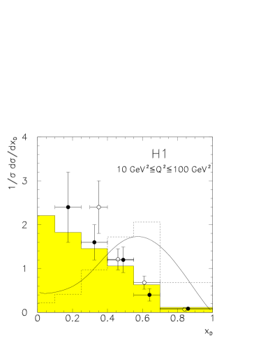
The charm structure function
The cross section measurements in bins of and can be expressed in the form of a charm structure function (fig. 5.21) analogous to . When compared with EMC data at , rises towards small . The data are consistent with NLO calculations based exclusively on the BGF process with gluon densities that describe the current HERA data. In the calculation both the renormalization and factorization scales are chosen to be . The dominant uncertainty in the calculation arises from the charm quark mass. The predicted changes by 15% when is changed by 0.2 GeV.
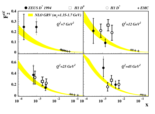
The measurements establish the boson gluon fusion process as the dominant one for charm production in DIS at , and thus the sensitivity to the gluon distribution function in the proton. The data are consistent with parton density parametrizations which were derived from the inclusive measurements, providing an independent cross check of the interpretation of the data in terms of parton densities.
The gluon density from charm production
In a new preliminary analysis [175] to determine the NLO gluon density from charm production H1 measures the visible cross section (corrected for detector effects) in the range , for mesons with laboratory and . The measured cross section is nb. The measured differential cross sections as functions of the kinematic variables , , , (not shown) are well described by the AROMA [172] charm generator and by a NLO calculation (program HVQDIS 1.1 [176] with the Peterson charm fragmentation function [177]).
is the proton momentum fraction carried by the gluon entering the BGF process. can in leading order be reconstructed from
| (5.13) |
Here is the charm quark’s 4-vector and it’s CMS transverse momentum. is the proton 4-momentum, and is the electron beam energy in the laboratory frame. The Lorentz invariant can be calculated from the charm quark’s energy and longitudinal momentum in the lab. frame. For BGF events it can be correlated with the quark scattering angle in the photon-gluon CMS, see section 7.4 and eq. 7.7.
Measured are charm mesons though, not charm quarks. Therefore the observable is defined by replacing with and with in eq. 5.13. is well correlated with [175].
The measured cross section as a function of is shown in fig. 5.22a. It is well described by the NLO calculation. The NLO calculation takes into account the gluon initiated processes and the quark initiated processes , , where the pair is produced from a radiated gluon. Using the NLO calculation for the cross section, the gluon density can be unfolded from the data. In the calculation is used, and the factorization scale is set to . The resulting NLO gluon density (fig. 5.22b) at an average scale reaches down to , and agrees well with a recent indirect extraction from the data [41]. Smaller values of could be probed with a larger angular acceptance for decays in the backward region, to be provided with silicon trackers. The ultimate limit is given by .
By reconstructing event-by-event , this measurement probes the gluon density locally in . In contrast, with the charm contribution is measured as a function of Bjorken , integrating over all . The comparison of the directly measured gluon density with the one extracted from the inclusive , and the agreement of with the prediction based upon such gluon distributions constitutes an important test of QCD with universal parton (here: gluon) densities. A similar test was obtained with dijet events in LO, see fig. 7.5.
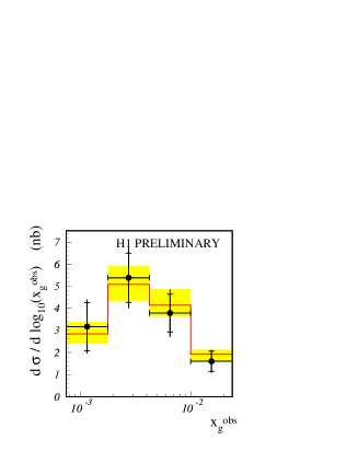
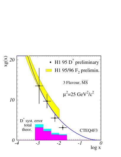
5.6 Bose-Einstein Correlations
Due to Bose-Einstein statistics, identical bosons prefer to occupy the same quantum state. In particle physics, the Bose-Einstein effect leads to an enhanced probability for identical bosons – like sign pions – to have similar momenta [178]. The shape and strength of their correlation function provide information on the production process.
As a measure of distance in momentum space for two particles with 4-momenta and with invariant mass one defines666This variable is traditionally denoted as . Here we use instead, because in DIS is already used for the virtuality of the exchanged photon.
| (5.14) |
assuming the particles to be pions. One measures the number of like sign charged particle pairs as a function of . This correlation function is compared to a function obtained similarly, but from a reference sample where Bose-Einstein correlations are absent:
| (5.15) |
As reference sample may serve a) unlike sign charged particle pairs, or b) pairs from different events (event mixed method).
If the particle emitting sources are distributed in space-time according to , a ratio
| (5.16) |
is expected for the Bose-Einstein enhancement. is the Fourier transform of and a normalization constant. The correlation strength is 0 for completely coherent emitters, and 1 for completely incoherent emitters.
The measurement at small , where the Bose-Einstein effect is expected, is notoriously difficult due to the finite double-track resolution of the tracking devices and due to pairs from photon conversions. The construction of a reference sample from the data introduces a residual bias. This effect is estimated by Monte Carlo, and cancelled by building the “double ratio”
| (5.17) |
The H1 data [179] are shown in fig. 5.23. A clear enhancement at small , attributable to the Bose-Einstein effect, is visible. The data cover , and . No dependence of the Bose-Einstein effect on the kinematic variables , or was found, nor a difference between the diffractive and non-diffractive data samples.

Different parametrizations of the effect have been fitted to the data. The traditional Goldhaber parametrization [180]
| (5.18) |
is derived from the the assumption of a static, spherically symmetric Gaussian source density . The parameter gives the size of the production volume. In high energy reactions, the sources are moving relativistically [181], and the assumption of a static source becomes invalid [182]. In the relativistic string fragmentation picture [183], an approximately exponential shape is predicted,
| (5.19) |
where the parameter is related to the string tension [184]. Alternatively, assuming a self-similar, scale-invariant pattern for perturbative QCD cascades, a power law is derived [185, 139]
| (5.20) |
Compared to the data (fig. 5.23), all parametrizations are acceptable, though the exponential and the power law ansätze give somewhat better results at low . A power law behaviour had been observed previously [186].
In order to compare with other experiments, the following results are obtained with the Gaussian (Goldhaber) parametrization, eq. 5.18 (table 5.5).
| reference sample | (fm) | |
|---|---|---|
| event mixed | ||
| unlike sign pairs |
With the event mixed reference sample, a lower value is obtained than with unlike sign pairs. Such a systematic effect has been observed also in other analyses. Other measurements in and lepton-nucleon interactions scatter between and , and and (see the compilation in [179]), but no pattern emerges. At least the extracted values of , including the HERA ones, can be said to be in the ball park of the length scale at which hadronization takes place, 1 fm. H1 finds marginal evidence for a dependence of on the charged particle multiplicity density , given as number of particles per unit pseudorapidity, . A strong multiplicity dependence of , roughly (with accuracy) for was seen in collisions [187, 188]. This is confirmed by the H1 data with a limited lever arm, .
Chapter 6 The Quark Fragmentation Region
6.1 Charged Particle Spectra
Comparisons with reactions
The physics issues that have been addressed with charged particle spectra in the Breit frame [189, 190, 191, 192, 193] are the study of fragmentation properties, QCD coherence effects, and scaling violations with the goal of determining . The advantage of experiments over experiments at fixed beam energies is that the scale variable can be varied continuously. Complications arise however from initial state parton radiation and from boson-gluon fusion events, which are absent in .
With the Breit current hemisphere a relatively small subsystem of the whole event is considered, (for most events ), which should be not much affected by the dynamics of the proton remnant (see sections 4.1 and 4.2 with fig. 4.3). The Breit frame current hemisphere of an event, the quark fragmentation region, is similar to one hemisphere of an event. Considering just the lowest order process, in interactions the outgoing quarks have opposite momenta of equal magnitude. The same is true for the incoming quark and the outgoing quark in the Breit frame of DIS. Furthermore, as in , the scale of the hard interaction, , also determines the phase space for QCD effects, given by the quark energy . In contrast, in the CMS . In the CMS it is therefore more difficult to disentangle a kinematic effect from a scale dependent QCD effect.
The scaled momentum variables of a hadron with momentum and energy are defined as (compare sect. 4.2)
| (6.1) |
with . In practice, one often approximates (massless kinematics). With the variable the soft part of the momentum spectrum at small , where the particle density is the largest, is expanded.
Fig. 6.1 shows the measured [189] and distributions of charged particles in the Breit current hemisphere for large and for small . is steeply falling, and is approximately Gaussian111 Qualitatively the Gaussian shape can be understood assuming that hadrons result from a chain of branching processes [194] (gluon coherence giving rise to a hump backed, approximately Gaussian, shape is discussed later). The branching stops, when there is not enough energy left to produce a hadron of mass . On average, (6.2) The give the energy fraction retained in each branching, and are assumed to be randomly distributed according to some splitting function . We expect that the hadron multiplicity is proportional to the number of branchings , hence a logarithmic growth of the average multiplicity with energy follows, (6.3) The energy left after branchings is (6.4) A hadron from this stage has energy with , where . We define the random variable , which is (6.5) can be written as a sum of random variables, and is thus Gaussian distributed for according to the central limit theorem, regardless of . The final hadron spectrum of all hadrons from all branching stages would then be the result of the sum of Gaussians with , where itself is a random variable. For not too large , this would give an approximate Gaussian, resulting from fall-offs at the kinematic boundaries at small and large . For large (large energy), a plateau const can develop, which translates into a rapidity plateau const. . When increases, soft particles (large ) are produced much more copiously. The hard part of the spectrum (large , small ) is approximately invariant of , “scaling”. This can be understood naively. If hadron production stems from a branching process with energy independent branchings, scaling at high is expected. At low , the reduction of the phase space forces a turnover of the spectrum, which happens at lower for larger initial energy.
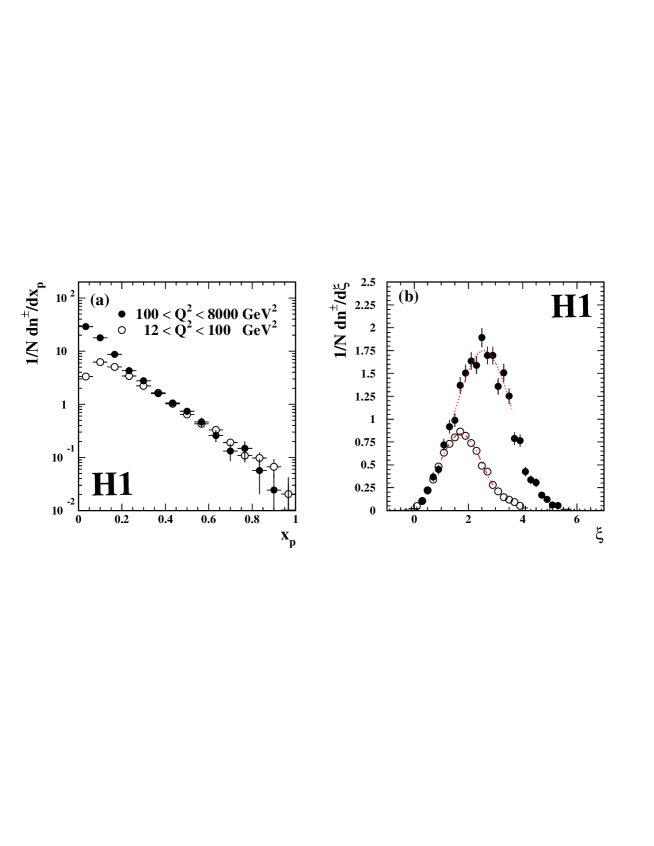


The evolution of can be effectively summarized by the dependence of the peak position and width of the Gaussian, shown in fig. 6.2. The average charged multiplicity (the integral over the fragmentation function) is shown in fig 6.3. An approximately logarithmic dependence of these variables on is observed:
| (6.6) | |||||
| (6.7) | |||||
| (6.8) |
and measured in annihilation at are within errors consistent with the data. For , also the total multiplicities agree, but at smaller , is significantly smaller in than in .
The deviation for can be attributed largely to LO QCD processes in , in particular to the boson-gluon fusion process which occur at small (hence small ) where the gluon density is large. For these events, the scattered quark may not be collinear with the photon, or may not even point into the Breit current hemisphere [196]. Its fragments are then emitted partly into the Breit target hemisphere222Consider the subsystem of the hard scattering subprocess with invariant mass (QPM events with massless quarks have =0). One can easily verify that for the momentum component of the hard subsystem is negative, pointing into the target hemisphere.. For charged particle production in the Breit current hemisphere appears to be similar to one hemisphere in annihilation, supporting the notion of universal quark fragmentation 333 In data the tails of the distribution deviate from a Gaussian. In the data, no significant deviation from a Gaussian has been found yet..
Predictions for the hadron spectra are available from a) perturbative QCD in the modified leading log approxiation (MLLA), where the transition to hadrons rests on the hypothesis of local parton hadron duality (LPHD); b) perturbative QCD in NLO, based on the QCD factorization theorem with universal, but scale dependent fragmentation functions; c) event generators with their sophisticated schemes to model perturbative QCD evolution and hadronization. They will be compared to the data in the following.
MLLA + LPHD predictions
The MLLA+LHPD derivation of the spectrum is discussed in [90, 197, 198]. The spectrum of partons in a parton cascade initiated by a quark of energy (and related virtuality) is calculated perturbatively in the modified leading log approximation (MLLA), including colour coherence. The cascade is calculated down to a low cut-off for the parton virtuality. It is then assumed (the hypothesis of local parton hadron duality, LPHD) that the final state hadrons follow the same spectrum, up to a constant factor. The predicted spectrum has a “hump backed” form of approximately Gaussian shape around the peak. On the other hand, when coherence effects are neglected, and a plateau =const. should form in the soft region, until the kinematic limit is reached at a scale . Coherence suppresses soft parton radiation, thus depleting the plateau at large – a “hump backed” plateau is formed444 A flat plateau =const. implies also a flat rapidity plateau, =const., since . A hump backed distribution therefore results in a depletion for . A dip in the rapidity distribution has been measured also in annihilation [199, 200]. The observation of a dip for 2-jet like events in annihilation provided evidence for soft and collinear gluon radiation [199]..
Analytical formulae in their various approximations for the spectrum are in general quite lengthy [90, 197, 198]. However, for large energies and concentrating on the main part of the spectrum , without the tails, the peak and width of the Gaussian are predicted to evolve with as [201]
| (6.9) | |||||
| (6.10) |
The constants are , with and ; they depend on the number of colours, , and the number of flavours, (here ). accounts for higher order corrections and is expected to be of order 1. is an effective scale for the evolution.
It is not a priori clear that the above MLLA+LPHD calculations for showering quarks can be applied to data, where BGF events play a rôle at small . A good combined fit to the H1 data is obtained though, yielding and , in agreement with an analysis of combined data, for which and was obtained [201].
It should be noted that the existence of a hump backed plateau, fig. 6.1, does not prove colour coherence effects. At finite energy, a hump backed, approximate Gaussian shape for the hadron spectrum can also be obtained in Monte Carlo simulations without coherence and with an independent fragmentation model [197]. One may argue that for an incoherent shower the turn over of the plateau happens at a scale . This point would define , hence , in contradiction to the slower growth of the data and of the MLLA prediction. However, in an incoherent shower model with string fragmentation, also a slower growth close to the data can be obtained [191]. Furthermore, in [197] it is demonstrated how string fragmentation can turn a flat plateau for partons into a hump backed one for hadrons. String fragmentation appears to compensate for negligence in the perturbative evolution. On the other hand, the growth of the average charged multiplicity with is less well described by string fragmentation with an incoherent parton shower [191].
Invariant energy spectra and the soft limit
Based upon MLLA+LPHD, the spectra from fragmenting quarks have been calculated also in the Lorentz invariant form
| (6.11) |
to study the small momentum limit [202]. The calculation agrees well with data. One salient feature is that for the calculated spectra do not depend on the energy of the fragmenting parton. The invariant spectra from H1 [190] are shown in fig. 6.4. The particle momentum is measured in the drift chamber. Its energy is set to , following the presciption in [202], where the “particle mass” is given by the mass cut-off of the parton shower, taken to be .
Comparison of the MLLA+LPHD prediction for fragmenting quarks, which has been shown to agree with data [202], with the data is hampered by the presence of BGF events. At low , the prediction is far off the H1 data [190], see fig. 6.4a. That effect can be reduced by a special anti-BGF event selection [190], which is based on the calorimetric energy seen in the Breit current hemisphere. That selection reduces the discrepancy at low . At large , where the discrepancy is smaller, there is little change after that cut, see fig. 6.4b. This study shows that in the Breit frame spectra there are fewer fast particles than in events at the same energy. The difference is presumably due to BGF events that are absent in . For larger , where the BGF contribution decreases, also the difference decreases.

The prediction of an energy (here: ) independent soft spectrum is confirmed – the measured spectra converge for , independent of (fig. 6.4c). It can also be noted that a calculation with fixed , instead of a running , is clearly untenable (figs. 6.4a,b). A meaningful extraction of is however not possible yet, because the calculations are available only in LO.
In the same H1 analysis [190], the KNO mulitplicity distribution was studied in the Breit current hemisphere. KNO scaling was found to be broken; at low the distributions broaden, and deviate the most from the approximately scaling data. Again, BGF events and the limited rapidity range can be held responsible for this observation. It would be interesting to test also KNO-G scaling [203], which is a reformulation of the KNO form, valid for discrete distributions (like multiplicities) at finite energies.
Scaling behaviour
The scaling behaviour of the spectra in the Breit current hemisphere are best studied by displaying the dependence of the normalized hadron cross section for fixed , where is the event cross section. With the large range of accessible at HERA, the scaling behaviour can be studied in a single experiment. Ultimately, could be extracted from such measurements [153].
The ZEUS data [192], covering are shown in fig. 6.5. The spectra were found to be almost independent of for fixed [189, 192]. Approximate scale independence is observed for : the cross section does not depend on . For smaller , the cross section increases strongly with (compare also fig. 6.1a). These effects are well described by the ARIADNE 4.08 [86] event generator; in LEPTO 6.5 [81] the scale dependencies are too strong, see fig. 6.5. Possibly the strong coupling parameter for the final state parton shower in LEPTO can be adjusted to describe the data.

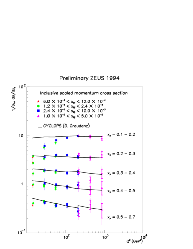
In fig. 6.6 new preliminary ZEUS data (1995) [193] are shown together with lower statistics H1 data (1994) [190] for . They agree very well. The data agree also very well with data from annihilation (corrected for and decay products, and divided by 2), supporting the notion of universal quark fragmentation in this kinematic region. The measured cross sections at small exhibit clear scaling violations with a positive slope. It is not clear however that this effect is due to the expected scale dependence of the fragmentation function in perturbative QCD. These expectations will be discussed now.

The spectra have been calculated [209] according to eq. 5.9 in NLO perturbative QCD (program CYCLOPS [204]) by folding parton density functions (here [210]) with the NLO matrix element for parton production and a NLO fragmentation function [211] for parton fragmentation into hadrons. All of these ingredients are scale dependent. was used.
The calculation agrees well with the data in the kinematic region shown in fig. 6.6, and . In this regime, the expected scaling violations are small, and can hardly be established with the present precision of the data. With higher precision data, and with a larger lever arm both at higher and smaller , the predicted scaling violations will be measurable. It will be very interesting to study to what extent this effect is due to the scale dependence of the fragmentation function, the matrix element, or the parton densities.
The fragmentation function picture has its limitations [209]. The fragments must not be too far separated in rapidity from the parent parton, assumed to fragment independently. It is estimated that the hadron rapidity in the Breit system should be above some minimal value , with . The condition , translates into a lower bound on ,
| (6.12) |
with the transverse mass , typically of . Furthermore, hadron masses are not taken into account with fragmentation functions. The calculation thus must break down when approaches . Indeed, the NLO calculation would by far overestimate the data in a region where and [209], see fig. 6.5. We note however deviations also at and , where the NLO calculation should be reliable according to eq. 6.12.
6.2 Event Shapes
Definition of event shape variables
Information on the shape of events, - pencil-like, spherical, cigar-like, planar etc. - is conveniently given by simple functions of the hadron momenta , . Measurements of such event shape variables provide information about both perturbative and non-perturbative aspects of QCD. Due to the large kinematic range covered, HERA is particularly well suited to study their scale dependence, for example on energy, and by that means disentangle the two contributions. Furthermore, provided the non-perturbative part can be estimated, the strong coupling constant can be extracted.
First measurements at HERA of the event shape variables thrust , jet mass parameter , and jet broadening parameter are reported by H1 [212]. The measurements are restricted to the Breit frame current hemisphere in order to avoid complications from the not so well understood region towards the proton remnant. The energy of the scattered quark in the Breit frame (in the QPM), , provides the scale for the process. values between 7 and 100 GeV are covered.
The variables are defined by
| (6.13) |
For the thrust calculation, the unit vector , defining the direction of a thrust axis, is varied555H1 has also measured the thrust for fixed thrust axis, defined by the virtual photon. in order to maximize , the normalized longitudinal momentum sum of all particles . for a collinear event configuration, and for a spherical configuration. Thrust measurements are usually expressed in , so that low values correspond to pencil-like events, as for the other event shape variables.
Thrust measurements
Here we shall concentrate on the thrust measurements, see fig. 6.7; the conclusions from the other shape variable measurements are similar. The measured mean value decreases with increasing , the events become more collimated. The thrust distribution as well as the mean thrust and their energy dependences are well described by the LEPTO model (version 6.1) [81], which incorporates a perturbative phase with the LO QCD matrix elements and leading log parton showers, and the Lund string model for hadronization.
Qualitatively, data from annihilation [213, 207, 205, 208, 206] follow the same trend as the data, but are systematically higher at small energies, GeV. One would actually not expect exactly the same distributions, partially because in the full event with two hemispheres is used666Note that the thrust for a system of two identical back to back jets equals the thrust of a single jet.. Furthermore, the flavour compositions differ, and in there are processes contributing, namely initial state QCD radiation and boson-gluon fusion, which are absent in . In fact, the other shape variables () show bigger differences than thrust between and data.


Power corrections
It has been argued [101] that for any infrared safe variable the mean value (and higher moments) can be written as
| (6.14) |
The perturbative part is calculable in fixed order perturbation theory, depending only on and the choice of renormalization scale777For the purpose of extracting a meaningful, process independent , the calculation has to be done in fixed order perturbation theory to at least 2nd order (NLO).. The only energy dependence comes from the running , since there is no other intrinsic scale in perturbative QCD than . QCD radiation patterns would be identical at all energies, if were constant. If the shape variable is invariant against momentum scaling with a constant (like ), , the distribution of the event shape variable depends on only through the running :
| (6.15) |
because the first term on the right hand side vanishes. In reactions a dependence may arise however via the dependent parton densities.
Higher orders and hadronization effects are collected in the “power correction term” , which according to [101] scales approximately (in general with the power ). A plausibility argument for such a term is given below. In contrast to the perturbative term, this term does depend explicitly on the energy, because hadronization introduces a scale, given by hadron masses. The higher order perturbative effects are calculated with running down to a scale , with to avoid the divergence of for , and to maximize the perturbative evolution. A conventional choice is . Below the scale , the calculation uses a constant effective coupling , a free parameter, which has to be determined by experiment, and which depends on the choice of .
The NLO expressions with as renormalization scale are [101]
| (6.16) |
| (6.17) |
where , and flavours888It is not clear what should be used for in this situation. The lowest values of are above the charm threshold, the larger ones are above the bottom threshold. On the other hand, for the parton shower with many soft emissions only light flavours are expected to be active. In fact, in the multiplicity analyses in sections 5.2 and 6.1 was used.. The constant is predicted by the theory and depends on the event shape variable under consideration (see tab. 6.1). In the H1 analysis, the constants and are calculated in the scheme with the program DISENT [78]. For e.g. they are and .
With the ansatz eq. 6.14 a good fit to the H1 data (and , as well) is obtained (see fig. 6.7) with and as the only free parameters. The perturbative contribution decreases with energy due to the decreasing . The power correction is substantial, but decreases from at to at . The prediction from LEPTO for partons is higher and closer to the data than the NLO calculation (see fig. 6.7), because the LEPTO parton shower includes QCD radiation in principle to all orders in the leading log approximation. In the ansatz 6.14, the higher orders are part of the power correction term. Whereas the differential thrust distribution is well described by the LEPTO model, the NLO calculation (covering states with up to 3 final state partons) is insufficient, producing too narrow events at small , but approaches the data for larger . This is not surprising, as the large NLO correction to the LO in eq. 6.16 (NLO/LO = ) suggests important higher order corrections, which should decrease with increasing energy due to the running .
From the thrust fit one obtains for the two free parameters , and for the strong coupling extrapolated to the mass999 Note that eq. 6.17 is not any longer a pure power law , but is modified by corrections up to . A pure power law fit of would give a worse than the “QCD improved” expression eq. 6.17 [214].. Similar values are obtained from the other event shapes, see tab. 6.1101010According to [101], the power correction term for the jet broadening parameter should be . From a comparison of the H1 data with the DISENT NLO calculation the extra term cannot be supported [212].. Assuming the power corrections to be universal (same for all shape variables), a combined fit to the thrust and jet mass data yields [212]; one has to admit however that the small combined statistical error disregards the fact that the data samples that enter the different distributions are the same, not at all statistically independent. To be on the safe side, one should quote 0.003 as statistical error instead. The obtained value agrees with the world average [14] with an error of similar size as in other determinations (see tab. 6.1 and [215]).
It is quite remarkable that the ansatz 6.17 gives consistent values for , and within 20% the same constant for all investigated shape variables. Furthermore, similar values are being obtained in shape analyses of data, see table 6.1. These encouraging results support the concept of universal power corrections, which deserves further investigation of its origin in QCD, and of its limitations. Besides new insights into hadronization, a better understanding would also improve the measurements. Recently also “power corrections” for the event shape distributions, not just the mean values, have become available [216]. It would be very interesting to compare these calculations to the data.
Naive model for power corrections
The power behaviour can be made plausible [75] with the simple tube or longitudinal phase space model [217] for hadronization. In this model a colour connected pair of partons with total energy produces two back to back jets of hadrons with energy each, where the hadrons are distributed uniformly in rapidity and according to a probability density function in transverse momentum. The resulting hadron distribution function is then , where gives the number of hadrons per unit rapidity. The energy and longitudinal momentum of one jet are given by
| (6.18) |
| (6.19) |
where is related to the average hadron by
| (6.20) |
Used were , , for light hadrons, and the quick convergence of towards . For a pencil like jet would have been expected; hadronization yields a negative correction of relative size , a simple power of the energy.
In this model we can calculate hadronization corrections to the otherwise vanishing and jet mass of the jet. According to the definitions eq. 6.13,
| (6.21) |
| (6.22) |
The corrections are proportional to , and twice as large for thrust as for the scaled jet mass squared, in accord with the constants for in tab. 6.1. The different values for in derived in [101] appear somewhat counterintuitive. One has to take into account however that the structure of DIS and events is more complicated than just two separating colour charges.
We can estimate the order of magnitude of the parameter from the data. From the seagull plot at low energies, where QCD effects are small, and for where intrinsic effects vanish, we estimate , see fig. 5.14. From measured hadron rapidity distributions one gets for the hadron density per unit rapidity [5], compare also fig. 5.8. That yields . In fact, a good description of event shape variables is obtained with power corrections parameterized with [75]. The fitted from the thrust analysis yields for the term in eq. 6.17 a coefficient of similar order, .
Chapter 7 Jets
7.1 Introduction
Amongst the spray of particles emerging from a high energy reaction the human eye can recognize collimated subsystems of hadrons, so-called jets (fig. 1.2). Jets are fascinating objects; they allow to view high energy quarks and gluons which are not observable as free particles due to confinement. As such they can be considered as the parton images imprinted on the hadronic final state. At short distances, partons can be treated as “asymptotically free”; their interactions can be calculated perturbatively. When the partons emerge from the confinement volume, they fragment into observable hadrons. At high energies, the hadrons will be collimated around the original parton direction. These hadron jets still carry information on the underlying partonic interactions.
Jets in DIS at HERA result from the scattered quark, and from additional QCD radiation either in the initial or the final state. Clean jet structures can develop due to the large available phase space ( up to 300 GeV). The main experimental challenge in jet studies is twofold: 1) to measure jet quantities like energy-momentum, charge etc., and 2) to relate them to the corresponding parton quantities. A good correlation between partonic and hadronic jet quantities is vital to allow perturbative QCD to be tested.
Jets at HERA have been studied with different intentions. The early measurements established clear jet structures in DIS [218, 219]. Fragmentation properties of quark and gluon jets have been studied by measuring jet shapes [220, 221]. Measurements of jet rates allow to study the partonic QCD mechanisms and to measure the parameters by which they are determined, like the strong coupling strength [222, 223], or the density of gluons in the proton [224]. It turns out that parts of the phase space for jet production, in particular at small and , is not yet well understood [225, 226, 227, 228]. The dedicated search for BFKL “footprints” with forward jets is covered in a chapter on low physics (section 8.4).
7.2 Jet Algorithms
For quantitative measurements jets need to be defined: a jet is the output of a jet algorithm. A jet algorithm prescribes how to combine objects (partons, hadrons, energy deposits, …) close in phase space to jets. It hinges on a resolution parameter below which jets cannot be resolved. The jet algorithm needs to be implemented not only experimentally, but also in the theoretical calculation for meaningful predictions. There exist several jet algorithms for different applications.
Clustering algorithms, like the JADE [229] or the algorithm [230], combine all final state particles into few jets, based upon a measure of distance. In the JADE algorithm, all particles with invariant mass
| (7.1) |
are merged to form new objects. (Experimentally, at HERA a pseudoparticle carrying energy and momentum of the unobserved proton remnant is introduced.) Here is the resolution parameter, and serves as reference scale. The final set of jets is obtained, when no further merging is possible.
In the algorithm two objects are merged, if
| (7.2) |
Particles can be merged also with the remnant. At HERA either is chosen [231], or is set to a fixed value, for example [225]. For small angles, the merging requirement becomes , where is the transverse momentum of the less energetic object with respect to the other one (hence the name algorithm).
For the cone algorithm [232] a distance measure in (pseudorapidity) - (azimuth) is introduced: . All particles inside a cone with radius (at HERA usually ) are combined to form a jet, if the resulting jet with respect to the proton axis is above a certain cut-off (usually a few GeV). The cone axis is chosen such that the inside the cone is maximized.
The result of a jet algorithm depends on the way masses are treated when combining objects (recombination scheme). Measured jets consisting of more than one particle always have a finite invariant mass, while most jets in NLO calculations are massless (they consist of just one massless parton). For this reason it is often found that the final result (e.g. ) depends on the chosen recombination scheme. A lot of effort is being spent on minimizing such effects. For the cone algorithm it also matters in which order objects are combined.
7.3 Jet Shapes
ZEUS has measured the internal structure of jets in DIS and has compared them to jets in other reactions [220]. One expects gluon jets to be broader than quark jets due to the larger colour charge of the gluon. In the laboratory frame, jets with and were selected with the cone algorithm () for events with . In most cases the current quark jet recoiling from the scattered electron will be selected.
One measures the average fraction of jet transverse energy inside a cone of radius around the jet axis as a function , defined by
| (7.3) |
is the number of jets in the event sample. by definition. The jet shapes are corrected for detector effects to the hadron level.
It is found that the jet shapes narrow as increases, as expected kinematically. (A jet will look narrower with increasing boost.) They show no significant dependence. (In a preliminary analysis of 2+1 jet events in the Breit frame, H1 found that these jets become broader towards the remnant [221].) The gross shape features are reproduced by the models investigated, PYTHIA 5.7 [233], LEPTO [81] and ARIADNE [86], but none of them provides an accurate description of the data over the entire phase space.
On average, DIS jets are seen to be narrower than jets from photoproduction. This can possibly be explained by the larger fraction of gluon jets in photoproduction, mostly from resolved processes, where a quark from the photon scatters with a gluon from the proton, . (However, multiple interactions between the proton and photon remnants could also lead to a a jet broadening in photoproduction [234]). A similar observation is made when comparing DIS jets to jets from annihilation [235], and to jets from interactions [236] with similar , see fig. 7.1. DIS jets and jets are predominantly quark jets and have the same universal shape within errors. They are narrower than the jets measured in interactions which contain a significant fraction of gluon jets.

7.4 The Strong Coupling
Analysis method
Considering the LO graphs for dijet production (fig. 7.2), the QCDC Compton (QCDC) and boson-gluon fusion (BGF) graphs, it is clear that the rate of events with 2+1 jets (the +1 refers to the remnant jet which escapes largely unobserved down the beam pipe) depends on the strong coupling constant , and on the parton densities in the proton. Inspired by the great potential to measure the behaviour of over the large span of accessible at HERA with high statistical precision, jet studies have focussed on the determination of right from the beginning of HERA data analysis. For this purpose one assumes parton densities that are constrained by other data.
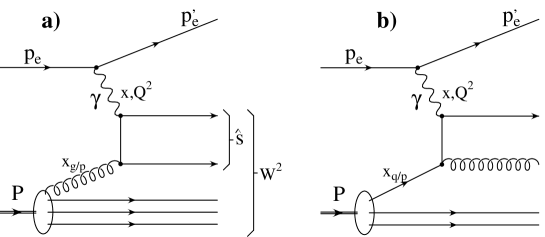
| DIS variables: |
|---|
The kinematics of the hard subprocess in 2+1 jet evenst is depicted in fig. 7.2. One defines the invariant
| (7.4) |
where is the invariant mass squared of the 2-jet system. In LO can be identified with the momentum fraction of the proton carried by the parton that enters the hard scattering, or for a quark or gluon.
At present the strategy is to measure with dijet data at relatively large , where the QCDC process dominates with well known quark densities at large . Dijet data at small , where the BGF process is the dominant one, are used to determine the less constrained gluon density at small , assuming a value for , see section 7.5. Best use of the information in the data will in the future be made from a combined determination of and the gluon density.
In the measurements the ratio of the number of 2+1 jet events to the number of all events ,
| (7.5) |
is determined as a function of . (H1 defines .) In the analyses the JADE algorithm is applied in the laboratory frame with resolution parameter =0.02. Another approach uses the dijet rate differential in the JADE resolution parameter , but no value has been quoted yet [237]. is being corrected for a) detector effects and b) hadronization effects to the parton level111The parton level needs to be carefully defined, see section 4.5., and is then compared to the QCD prediction in NLO:
| (7.6) |
and are calculable coefficients that depend on the kinematic conditions, the QCD renormalization and factorization scales, and on the parton densities. is determined from a comparison of the measured jet rate, corrected to the parton level, with the NLO prediction of eq. 7.6.
The analyses cuts are designed such that a) the observed jet rates are well described by the Monte Carlo used for corrections; b) the correction factors are reasonably small; c) the NLO prediction for partonic jets resembles the partonic jets found in the Monte Carlo generator. Jets from initial state parton showers complicate matters; to a large extent they are not covered by the NLO calculation.
Data analysis
The corrections for detector and hadronization effects rely mostly on the MEPS model (program LEPTO) [81], where the hard scattering at the photon vertex is calculated with the LO matrix element; higher orders are taken into account with leading log DGLAP parton showers. Hadronization is performed with the Lund string model [93]. Other programs (ARIADNE [86], HERWIG [82]) are used as cross checks. Fig. 7.3a shows [231] as a function of in comparison to the models. The data are corrected for detector effects to the hadron level. LEPTO describes this rate reasonably well. It is not understood why the other models do not describe this data at relatively large , where little theoretical ambiguity is expected.


The QCD calculations in fixed order perturbation theory are performed with the programs PROJET [238], DISJET [239], MEPJET [79], and DISENT [78]. PROJET and DISJET are no longer in use, because parts of the phase space at small and large were not fully included222The published ZEUS analysis [223] presented here was based on PROJET. It has been verified though that due to the cuts applied the effect on the extraction is negligible (less than 2 per mil) [240]..
In the following two paragraphs, typical features encountered in the HERA analyses are reported. One finds 2+1 jet events in the total event sample [219, 227], depending strongly on and also on the event and jet selection. The dependence of on for is well described by Monte Carlo (LEPTO 6.1) [219] and by NLO calculations (PROJET) [223]. With increasing , fewer structures are resolved as jets. According to the Monte Carlo (LEPTO 6.1), around 75% of matrix element 2+1 jet events are due to BGF for (50% for ), the rest is due to QCDC [219]. In LEPTO, around 50% of the 2+1 jet events originate not from the LO matrix element, but from the parton shower, that is mostly initial state radiation [222, 241]. The parton shower contribution is reduced at high [242].
The NLO correction to the LO prediction is roughly 20%, depending on the analysis details, in particular on [223]. Migrations between jet classes due to hadronization effects can be large: of 2+1 parton jet events and of partonic 1+1 events are correctly classified after hadronization [219]. The resulting corrections for hadronization are sizeable, around 30% [231]. Similar numbers are obtained for migrations due to detector effects. In general, smearing effects become less severe for larger . Therefore the analysis apply lower cuts, 120 for ZEUS [223] and 40 for H1 [231].
Two Lorentz invariants can be introduced to describe the jet kinematics, for example , the invariant mass squared of the two jets, and
| (7.7) |
The index denotes the jet from a particular parton. and . The approximate relation with the scattering angle in the parton-photon scattering frame (the rest frame of the two jet system, fig. 7.4a) holds for small jet masses and small . In the experiment one defines with . can be reconstructed from the measured jet angles and energies in the laboratory frame,
| (7.8) |


The LO matrix element for the QCDC process diverges , and for BGF with the familiar soft () and collinear () divergencies. It turns out that close to the collinear divergency (), more 2+1 jets are observed than expected from either the NLO calculations (see fig. 7.4) or the LEPTO simulation [227, 223]. In this part of the phase space the NLO corrections are largest, and according to the Monte Carlo, parton shower effects are most severe (apart from the LO BGF and QCDC events, QPM events with initial state parton showers can contribute up to 50% to the total 2+1 jet rate). The region , corresponding to small angles in the lab system with respect to the proton remnant direction, is therefore cut out for the determination of [223, 231]. H1 applies an additional cut , and requires in order to exclude the backward detector region which was not instrumented with hadronic calorimetry.
Results
From a comparison of the jet rate , corrected to the parton level, with the NLO expression of 7.6, is determined as a function of . ZEUS has measured in three bins from 120 to 3600 , and H1 (preliminary) in four bins from 40 to 4000 , see fig.7.3. The data are consistent with the decrease of with increasing scale according to the renormalization group equation. A fit to the data with the NLO expression for the running , eq. 2.8, with as free parameter yields the results in table 7.1. These measurement from jets at HERA agree with the world average [14].
| ZEUS | ||||
|---|---|---|---|---|
| H1 prel. | ||||
| world avg. | ||||
For the ZEUS result, experimental and theoretical systematic errors are given separately. H1 found that alternative recombination schemes than the ones used would increase by the amount quoted. The dominating systematic errors are the corrections for hadronization effects and the dependence on the choice of renormalization and factorization scales. The largest experimental systematic error is due to the uncertainty of the absolute calorimeter calibration, which is known to about .
It is estimated [243] that with a large amount of luminosity to be collected at HERA in the future, 250 , the errors on can be reduced to (stat.) and (syst.). Other algorithms than JADE may turn out to be advantageous in the future [231]. In any case, a good understanding of perturbative QCD beyond LO and hadronization will be mandatory to achieve a good precision on . For example, the puzzle why two otherwise respectable QCD models fail to describe the jet rate at the hadron level (fig. 7.3a) needs to be resolved.
7.5 The Gluon Density
The gluon density at small fractional momentum () had been extracted previously only indirectly from inclusive structure function measurements. A direct measurement of the gluon density is in principle possible via the measurement of 2+1 jet events from the boson-gluon fusion (BGF) process . The 2+1 jet cross section can in leading order QCD be described as the sum of quark initiated and gluon initiated processes, QCDC and BGF. Schematically,
| (7.9) |
Here and are the fractional proton momenta carried by the incoming quark and gluon. They are given in LO by , see fig. 7.2. and are coefficients that can be calculated perturbatively. The experimental challenge is to reconstruct by measuring . That requires to separate in the hadronic final state the hard subprocess from initial state parton showers and the proton remnant.
For the extraction of the gluon density , is assumed to be known and taken from the PDG world average. The contributions from the competing QCD Compton process (QCDC) , which is calculable using known quark density functions , and from wronlgy classified QPM events have to be subtracted statistically from the observed 2+1 jet rate.
Of particular interest is the gluon density at small , where no direct measurements exist. In order to access small values of ( in LO), small invariant jet-jet mass need to be resolved. The JADE jet algorithm resolves 2-jet events with . That defines the accessible phase space, and implies .
To reach lower values of than given by the canonical , the H1 analysis [224] uses the cone jet algorithm () applied in the hadronic CMS. For the jets is required. Since for massless objects
| (7.10) |
values of can be obtained. With the large , much lower values can be probed than with the JADE algorithm.
From DIS events at small ( ), 2+1 jet events are selected with in the laboratory frame. Their distance in (lab) pseudorapidity had to be smaller than . In the hadronic CMS, that cut translates roughly to . These angular cuts remove events affected by parton showers. is required. is reconstructed 1) as the invariant mass squared of all particles belonging to the two jets, and 2) from the jet directions (pseudorapidities ) measured in the hadronic CMS,
| (7.11) |
It is required that the two methods agree to GeV.
The selected 2+1 jet event sample covers and . According to the Monte Carlo (LEPTO), BGF and QCDC events are selected in a ratio 3:1. By unfolding the observed distribution, the (LO) gluon distribution at is obtained (fig. 7.5). The data extend the region previously covered by NMC [244], down to . This direct measurement of the gluon density confirms the steep rise of the gluon density at small which had been deduced from the structure function data (see fig. 7.5). A preliminary ZEUS analysis using a similar method gives consistent results [241], within large errors. We note that sizeable NLO corrections for jet production have been calculated [245].
Recent analyses focus on the direct determination of the gluon density in NLO [246]. Using the measured partonic jet rate (JADE algorithm) for from the H1 analysis [231] as input (see section 7.4), the extracted gluon density for is consistent within errors with results from structure function analyses [247]. Due to the phase space restriction implied by the JADE algorithm, not very small are probed, . Smaller values can be accessed by tagging gluon initiated BGF events with identified charm decays [175], see section 5.5.
Recent attempts to extract the NLO gluon density at small from dijet production at low and are facing a problem [228, 248]. There are about 20-30% more dijets in the data than expected from NLO calculations or from e.g. LEPTO with gluon densities as input that are compatible with the data. At face value, that would indicate a directly measured gluon density that is incompatible with the indirect extraction from the measurements. It could also be that there are effects contributing to jet production at small and that had not been taken properly into account. To clarify the situation, data on jet production are essential that do not contain any theoretical bias from the correction to the parton level. Such measurements are presented in the next section.
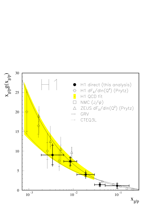
7.6 Jet Rates at Low
In a preliminary ZEUS analysis [228] that addresses the gluon density, the dijet cross section (cone algorithm in the laboratory frame with ) has been determined and corrected for detector and hadronization effects to the parton level using LEPTO 6.3. In the laboratory frame, was required to exclude the forward region. A cut was applied in the laboratory frame and in the CMS.
The shapes of the measured cross sections as a function of , , and in the CMS, and are well described by LEPTO and by NLO calculations [79]. However, the absolute dijet cross section is larger than predicted by NLO QCD (see fig. 7.6). Systematic effects cannot account for such a large discrepancy [228] .

The previous jet studies were aimed at the measurement of observables defined in QCD - the strong coupling constant and the gluon density. To that end regions of phase space where the data deviate from the theory - cast either into NLO calculations or Monte Carlo generators - had been carefully avoided. These phase space regions were found at low and low , and in the forward region close to the remnant [252, 228, 248]. The forward region at low is discussed in a special chapter on low physics, section 8.4. Here we shall discuss jet production at low , with ranging from the DIS regime down to photoproduction, . The object of these studies is a test of QCD and to explore the validity of QCD models for jet production. The data extend into a new phase space region in DIS, where the transverse momenta squared of the jets may exceed , . In such a situation it may be possible to probe constituents of the virtual photon at a scale given by the of the jet [253].
In a preliminary H1 analysis [226], low DIS events are selected with , where the scattered electron angle and energy are and . The data sample covers and . Exactly two jets are required, reconstructed with the cone algorithm () in the hadronic CMS and with transverse momenta . The remnant is not counted. The pseudorapidity difference between the two jets has to be less than 2. In the CMS of the scattering parton and the virtual photon, the jet angles with respect to the photon axis are given by
| (7.12) |
The requirement thus excludes very forward jets, because , or . Measured is the dijet rate , the fraction of DIS events that fulfil the dijet requirements. The rate is corrected for detector effects to the hadron level (fig. 7.7 top). The dijet rate increases from 4 to 10% for between 10 and 100 .
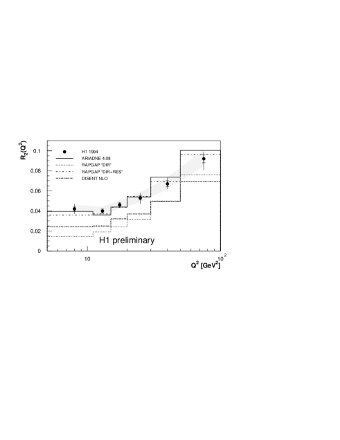
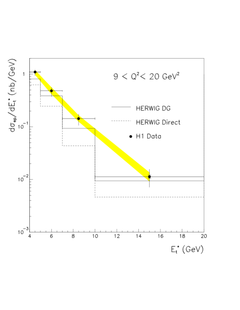
The data are compared to different QCD models, see fig. 7.8. In RAPGAP DIR (direct) [83], the virtual photon interacts directly with a proton constituent. The hardest interaction (with the highest ) takes place at the photon vertex and is modelled with the LO QCD matrix element. Softer emissions are generated with DGLAP parton showers. In RAPGAP DIR+RES it is assumed that there exists an additional contribution from so-called resolved processes, where the structure of the virtual photon is resolved by a hard scale, in this case the jet with [255]. The hard interaction takes place further down the ladder between (evolved) partons from the photon and from the proton. Virtual photon parton densities were taken from SaS-2D [256]. The resolved contribution breaks the ordering in the parton evolution.

In the colour dipole model (CDM, program ARIADNE [86]), gluon emission stems from a chain of independenly radiating colour dipoles. The amount of radiation depends on the parameters that describe the extendedness of the proton remnant colour charge, and on the extendedness of the colour charge of the scattered quark, which is determined by . Emitted partons are not restricted to obey ordering. The radiation pattern thus shows similarity with BFKL evolution [87, 88].
The data cannot be described by direct interactions only (fig. 7.7 top), when conventional DGLAP models are applied. At low (and also small ), the measured dijet rate is more than a factor two above a model which contains direct interactions only. At low around 50% of the dijet rate is “missing”, that amounts to of the total event rate. Also a NLO QCD calculation for parton jets with DISENT [78] falls short of the data. Hadronization is unlikely to account for the difference, because the difference between hadronic and partonic dijet rates in the Monte Carlo was found to be for GeV. The discrepancy diminishes with increasing (and also inreasing ). The models where the hard interaction is not tied to the photon vertex, implementing either a resolved component of the virtual photon, or colour dipole radiation, provide a good description of the data.
In a similar analysis the single inclusive jet cross section (algorithm with ) has been measured as a function of jet and pseudorapidity for events with and [225]. The data are corrected to the hadron level. It was found that when the transverse energy squared of the jet exceeds , conventional models (LEPTO 6.5 [81], HERWIG 5.9 Direct [82]) with direct photon-parton interactions alone undershoot the data (fig. 7.7 bottom) by a large amount. A better description of the data is obtained when contributions are taken into account where the hard scale provided by the jet serves to resolve partons inside the virtual photon (HERWIG 5.9 DG, with resolved photon component), or by the colour dipole model (ARIADNE 4.08 [86]).
In summary, the mechanism for jet production at small and is not yet very well understood. It appears that for regions of phase space where the jet is larger than the conventional DIS framework, where the virtual photon resolves partons inside the proton, ceases to be valid. Instead, the high of the jet could resolve both structures of the proton and of the virtual photon. We note that the linked dipole chain model [24, 89] should be able to treat both situations consistently where the jet is smaller or larger than . This field of research will continue with more detailed measurements. It has to be seen also in connection with “small-” physics, to be discussed in the next chapter 8. Are these models alternatives to genuine “small-” effects, as expected from BFKL evolution, or are they just a different language for the same effect? It remains to be seen whether the competing models are actually consistent with the large body of other hadronic final state data, or whether they can describe just one facette of the hadronic final state.
Chapter 8 Low- Physics
8.1 Introduction
Amongst the most interesting issues of HERA physics is QCD in the newly accessible regime of small , see section 2.5. The observed rise of the structure function towards small suggests a strong increase of the parton density in the proton, but what is its dynamical origin? Is DGLAP evolution sufficient to account for the data, or is BFKL dynamics at work, at least to some extent? The structure function measurements are probably too inclusive to answer such questions unambiguously. Complementary measurements of the hadronic final state provide more detailed information on the reaction, which may help to uncover the underlying dynamics.
In the simple quark parton model, a quark is scattered out of the proton by the virtual boson emitted from the scattering lepton. QCD modifies this picture. Partons may be radiated before and after the boson-quark vertex, and the boson may also fuse with a gluon inside the proton by producing a quark-antiquark pair. In fact, the parton which is probed by the boson may be the end point in a whole cascade of parton branchings. This parton shower materializes in the hadronic final state, allowing experimental access to the dynamics governing the cascade.

Though there may be other dynamical features to be discovered that leave their footprint in the hadronic final state (see for example section 7.6 on the virtual photon structure or chapter 9 on instantons), most dedicated small measurements have concentrated on the predicted signals for BFKL evolution. The leading log DGLAP resummation corresponds to a strong ordering of the transverse momenta (w.r.t. the proton beam) in the parton cascade (). In the BFKL regime, the transverse momenta follow a kind of random walk () [257]. The longitudinal momentum fractions are ordered according to for BFKL and for DGLAP.
A radiated parton (or any other object) with CMS momentum fraction and longitudinal and transverse momentum components is to be found at CMS rapidity
| (8.1) |
For fixed and fixed , the CMS rapidity is determined by . Here the relations and in the CMS have been used (with the proton direction along the axis). Finally,
| (8.2) |
For DGLAP evolution the phase space for parton radiation between the remnant and the current is restricted by ordering. A generic signal for deviations from DGLAP evolution is therefore enhanced activity in the central and forward CMS rapidity region, between the current system and the proton remnant. The observables which have so far been exploited are the following:
Apart from a few theoretical calculations in the resummed DGLAP and BFKL schemes, and calculations in fixed order perturbation theory (mostly NLO), predictions for the final states observables can be derived from Monte Carlo models only. Theoretical calculations have the advantage that their theoretical input is well defined. However, most of them (an exception is presented in section 8.3) neglect hadronization, making it difficult to compare them with data. On the other hand, the draw back with Monte Carlo models is that often their complexity and their flexibility to model hadronization makes it difficult to pin down which feature of their theoretical input is actually being tested when comparing to data.
HERWIG [82] and LEPTO [81] which are based upon leading log DGLAP parton showers are used as representatives for DGLAP evolution with strong ordering. Unfortunately a Monte Carlo program based upon BFKL (or CCFM, which in the limits of small and large approaches the BFKL and DGLAP evolutions) dynamics is not yet available for reactions, though there exist some promising developments in that direction [267, 268, 22]. Rather, the DGLAP model predictions are contrasted with the colour dipole model ARIADNE [84, 86]. In certain aspects the CDM description of gluon emission is similar to that of the BFKL evolution [87, 88]. In particular the gluons emitted by the dipoles do not obey ordering along rapidity (see section 4.4).
8.2 Energy Flows
The measurements of the transverse energy flow [127, 113, 114, 115, 130, 269, 128, 270, 271, 272] have had a great influence on our understanding and modelling of the hadron production mechanism in DIS. It had been noted already in the early papers [113, 128] that some standard QCD models for the hadronic final state failed to describe the measured energy flows, in particular at low (see also section 5.1). The MEPS model (LEPTO 6.1), based upon the LO QCD matrix element with DGLAP parton showers and string fragmentation, undershoots the H1 data [113] by a factor two in the “forward region”, towards the proton remnant (fig. 8.2 a). In the following years, the energy flow and it’s dependence on kinematic conditions has been studied in great detail.
The “forward” measurement close to the beam hole at the edge of the calorimeter acceptance at , corresponding to , is very difficult, as particles are lost in the beam pipe, and backscatter from lower angle particles hitting dead material produce background in the forward calorimeter region [273, 274, 275]. An independent measurement is provided by ZEUS, where the instrumentation and dead material distribution in the forward region are quite different. Fortunately, the data from ZEUS [270] agree with the H1 data (see figs. 8.2b and 8.4), confirming the “forward energy crisis” [276].


The discrepancy between data and LEPTO, considered as the reference model for hadron production, triggered further investigations, both theoretically [258, 277] and experimentally [114, 115, 270, 271] whether low effects, for example BFKL dynamics, could be held responsible for the excess. Shown in fig. 8.2 b are also results of calculations [258] based upon either BFKL or DGLAP parton dynamics. Qualitatively, much more is expected from BFKL than from DGLAP evolution, roughly at the level of the data. However, these calculations do not include hadronization, and are therefore not directly comparable to the data.
The flows have now been measured over a wide range of and [114, 115, 271], and are presented in the hadronic CMS to eliminate the transverse boost introduced by the scattered electron. The latest preliminary H1 data [115, 278] (fig. 8.3) also employ the plug calorimeter [279] installed at small angle behind the liquid argon calorimeter, extending the acceptance far into the target region. The plug data have large errors due to the large amount of dead material along the line of sight to the interaction vertex, between 2 and 4 nuclear absorption lengths.
The flow is plateau-like ( per unit ) at small and , and becomes more peaked in the current region at larger and . The average () measured centrally () in the CMS rises with decreasing (see fig. 8.4)111The dependence for fixed implies also a dependence. In fig. 5.8 it is shown that the average at central rapidity increases with in DIS, and that this behaviour is in agreement with data from hadron-hadron collisions. A deeper understanding of production in DIS might also be benefitial for the understanding of the hadron-hadron data, which so far could be just parametrized phenomenologically. . This behaviour is predicted for the partonic from the BFKL calculation, whereas for DGLAP evolution the opposite is expected [258]. CDM gives still the best overall description of the data. The DGLAP based models, MEPS and HERWIG, have developed and now give also a reasonable description of the data (fig. 8.3).


In order to draw conclusions from comparing the data with partonic QCD calculations, hadronization effects need to be estimated from Monte Carlo models. The partons produced in the CDM give about twice as much in the central rapidity region as the ones emitted from the ordered cascades in MEPS and HERWIG, see fig. 8.5a [261], which can be traced to the fact that hard gluon radiation is much more abundant in CDM, see fig. 8.5b [281]. However, the observable particles emerging after hadronization give rise to very similar flows. The flow predictions of the different models cannot be well discriminated with the present data. While hadronziation adds relatively little () to the partonic for CDM, most of the () is generated by hadronization for MEPS and HERWIG. It is noteworthy that CDM and MEPS use the same Lund string fragmentation model for hadronization. In addition, the partonic and the hadronic are well correlated event-by-event in CDM, as opposed to the other models [261].
With the data alone, the hadronization ambiguity cannot be resolved. The situation is summarized in fig. 8.6. The data rise with falling and agree with both the ordered and the unordered Monte Carlo models for hadrons. BFKL predicts also a rise, as is seen in the CDM partons, but at a somewhat lower level. Apart from the normalization, the data are consistent with a BFKL interpretation, assuming hadronization effects as given by CDM. The DGLAP model partons produce much less than CDM, and have the opposite behaviour, as expected for DGLAP evolution [258]. However, the data are also consistent with DGLAP evolution, when large hadronization effects are assumed. How do they arise?


In LEPTO 6.4 changes to the non-perturbative part were introduced to simultaneously describe the large flow seen in the data, and to explain the rapidity gap events [104, 105, 102, 103] without invoking the explicit exchange of a Pomeron [109]. In the new concept of soft colour interactions (SCI), colour quantum numbers may be exchanged between the outgoing partons after the hard interaction, leading to a reconfiguration of the fragmenting strings (see section 4.6). This may result in colour neutral subsystems, separated by a rapidity gap from the rest of the event after hadronization, or it may enhance the flow, when strings are spanned back and forth (fig. 4.14). Also the treatment of the remnant fragmentation has been changed for events where a sea quark is hit (new sea quark treatment - SQT). Instead of recombining the sea quark partner (for example a quark in case a sea quark was hit) within the remnant to form a hadron, a fragmenting string is now stretched between the hit sea quark and the remnant. At large these effects are minor, but at small they are significant, see fig. 8.7. As long as the new SCI concept has not been ruled out by other data – from detailed studies of rapidity gap events, for example – it has to be taken seriously. The SCI does not only offer an explanation for the rapidity gap events and the large flow, but has also been advocated [282] to explain the large production rate of heavy quarkonia in interactions at the Tevatron [283]. Presently the SCI model has difficulties describing the thrust of the hadronic final state in rapidity gap events, but so do the other models based upon Pomeron exchange [112]. Further data will be necessary to discriminate the Pomeron exchange and SCI models.
In the CDM hadronization effects are much smaller, because gluon radiation is more abundant, and less energy remains for hadronization. The large hadronization effects in HERWIG can possibly be explained by its very simple cluster fragmentation scheme. When there are few partons, the masses of parton pairs (clusters) to be fragmented tend to be large. In the cluster fragmentation model, they undergo a two-body decay according to phase space, leading to large transverse energies. The same mechanism leads to a significant fraction of rapidity gap events which are “not exponentially suppressed” in HERWIG without Pomeron exchange or soft colour interactions. In a later version (HERWIG 5.9) this problem is being addressed by allowing large mass clusters to split longitudinally before they decay.

8.3 Transverse Momentum Spectra
Not yet well understood hadronization effects, however interesting they may be, precluded strong conclusions on the underlying parton dynamics from the transverse energy flow measurements. It has been shown that single particle transverse momentum () spectra represent a more direct measure of the partonic activity, and corresponding measurements have been suggested [284, 261].
To answer the question whether the observed in the data is generated predominantly by parton radiation or by hadronization, inclusive spectra are considered. Hadronization should produce typical spectra which are limited in , while parton radiation should manifest itself in a hard tail of the distribution. To test this idea particles from a “central” (in the CMS) interval are examined. Simulated events are compared which have similar hadronic () in that interval, with either a large or small contribution from partons. The parton dominated events indeed exhibit a harder spectrum than the hadronization dominated ones (s. Fig. 8.8a), regardless of the mechanisms employed for parton evolution and hadronization. Different parton evolution scenarios which differ in the production of hard gluons (for example BFKL vs. DGLAP, or CDM vs. MEPS/HERWIG, see fig. 8.2) can thus be discriminated by the number of high-hadrons which are produced. In a similar fashion the distribution of the measured centrally could be used for discrimination [261] (fig. 8.8c). Preliminary H1 data [115] favour the CDM over the other models, but the study of systematic errors has not yet been completed.


H1 has measured [118] the charged particle spectra as much central in the CMS () as the detector acceptance allows222The measurement relies mostly on the central tracking device; when systematic effects presently hampering the forward tracker are mastered, the measurable rapidity region could be enlarged by one unit of rapidity towards the remnant.. Measured is
| (8.3) |
where the differential cross section to produce a hadron with transverse momentum in a pseudorapidity interval is normalized to the differential event cross section for given . In the measurement, the differential cross sections are averaged over certain small bins.
The data are compared in fig. 8.9 to models with suppressed (LEPTO 6.4, including SCI and new SQT; HERWIG 5.8) and unsuppressed (ARIADNE 4.08) radiation patterns. At “large” and (here “large” means GeV2 and ) all models provide a good description of the data. At smaller and , LEPTO and HERWIG fall significantly below the data for GeV. ARIADNE gives a good description of the data over the full kinematic range. The shortfall of the models with suppressed gluon radiation indicates that at small there is more high parton radiation present than is produced by the models based upon leading log DGLAP parton showers. These models are closer to the data in the current region, or when all charged particles are considered, including the soft ones [118], see fig. 5.7.

In a preliminary analysis of the H1 forward tracker, data have been obtained also in the “truly central region”, . In fig. 8.10 the charged particle spectra are shown for three different ranges. At central rapidity, , the spectra from photoproduction and DIS are similar. Towards the photon fragmentation region, the DIS spectra become harder than the photoproduction data. Apparently, in that region, the virtuality influences the hardness of the spectrum, while there is little influence in the central region. A similar conlusion has been arrived at from the study of the flow, see section 5.1. The DIS data are well described by the CDM. LEPTO becomes too soft away from the current region. The prediction by the photoproduction model PHOJET [285] describes the photoproduction spectra well.

Theoretical calculations for the charged particle spectra have become available [287], where a cross section to produce a parton is folded with an experimentally known fragmentation function [211] to produce a hadron with momentum fraction from the parton , see fig. 8.11a. Monte Carlo models for hadronization are thus avoided. Symbolically,
| (8.4) |
The parton cross section is divided into a conventional part where gluon emissions in the ladder are ordered, and a part with unordered emissions, which is calculated with the BFKL equation (see fig 8.11a). The H1 data at low are well described by this calculation, see fig 8.11b. The absolute normalization for the BFKL part is obtained by requiring that the calculated parton cross section would match the measured H1 forward jets [288] at the hadron level, see section 8.4. We note that this normalization neglects the effects of the jet algorithm and hadronization effects, both of which are not included in the single parton cross section calculation. Without the BFKL part the calculation is by a factor below the data. Both predictions show little dependence on the choice of the factorization scale for the fragmentation function.
For the “no BFKL” calculation the LO cross section for three partons was used, where the main contribution is the diagram with the from the quark box plus one additional gluon, see fig. 8.11a. A complete NLO calculation is still missing. DGLAP evolution was neglected, because the kinematic conditions severely disfavour DGLAP evolution. DGLAP evolution is not possible between the parton and the photon if due to strong ordering. For the curves shown in fig. 8.11b this condition is approximately fulfilled, , because a leading hadron carries on average about half of the fragmenting parton’s momentum, .


An even better signal is expected when the single particle detection capability could be extended further towards the proton remnant [281, 266]. Typically at HERA, the central trackers are limited to , and the forward trackers to . An upgrade with a forward silicon tracker could cover angles [281]. Alternatively, one can detect single photons or s in the calorimeters, which have acceptance for typically .
H1 has measured “forward” production [289], where the meson is detected via the electromagnetic showers of their decay photons in the H1 forward liquid argon calorimeter [289]. The ’s have been selected in the laboratory frame with , , and (data with other cuts exist as well) in order to enhance the phase space for BFKL evolution. The number of such ’s increases with decreasing Bjorken , see fig. 8.12. The models studied, MEPS and CDM, agree at large with the data. The rise towards small is only followed by CDM. Calculations for forward production exist in principle [266, 287], but need to be repeated for the kinematic conditions of this H1 measurement.

Coherence effects, which can be taken into account by angular ordering, are expected to modify the BFKL behaviour. They are included in the CCFM equation [20]. Predictions for the hadronic final state at low based upon the CCFM ansatz are now emerging [22]. In general, there is less diffusion in CCFM than in BFKL. The number of soft emissions is much reduced in CCFM when compared to BFKL, due to angular ordering (fig. 8.13). For appreciable transverse momenta, the differences are not so big, affecting mainly the high multiplicity tail.

The CCFM equation has been reformulated in the linked dipole chain model (LDC) [24]. First results from a Monte Carlo generator implementing the LDC in the ARIADNE framework are promising [89]. The critical distributions, flows and spectra at small , are much better described than with LEPTO, though the agreement with the data is not quite as good as with the CDM [89].
8.4 Forward Jets
The classic signature for BFKL evolution in the hadronic final state are so-called “forward jets” [259, 260] close to the remnant, that is “forward” for the HERA detectors. The selection criteria are designed such as to suppress the phase space for DGLAP evolution, and to maximize it for BFKL evolution. , the ratio between the jet energy and the proton beam energy , is required to be as large as possible, since BFKL evolution between the jet and the quark box requires to allow for strong ordering along the ladder (see fig. 8.1, where the forward jet is thought to emerge from a radiated gluon close to remnant). The transverse momentum has to be close to (). The phase space for ordered DGLAP evolution () is thus much reduced, whereas it is still open for unordered BFKL evolution. An enhanced rate of events with such jets is thus expected in the BFKL scheme [259]. The experimental difficulty is to detect jets close to the beam hole in the proton direction in the forward calorimeter.
Previous measurements by H1 [114] were limited in statistics, but were consistent with BFKL calculations [290]. In the preliminary analysis of the larger statistics sample from 1994 [288] forward jets with are selected with the cone algorithm (cone radius ) in the HERA laboratory frame within . The transverse jet momentum requirements are and a lower cut-off 3.5 GeV. The forward jet rate, corrected for detector effects to the hadron level, increases sharply with falling , see fig. 8.14. This is expected from BFKL calculations, in contrast to calculations without the BFKL ladder [291]. The behaviour of the data is well described by the CDM with the unsuppressed gluon radiation pattern. The DGLAP based model MEPS cannot describe the rise towards small when soft colour interactions are switched off. When soft colour interactions are activated however, without changing the parton dynamics, MEPS comes up rather close to the data. A good description of the forward jet rate is also provided by RAPGAP including a resolved (not point-like) component of the virtual photon [255]. The physical significance of this fact is still being debated.


Hadronization effects may play an important rôle for small , where it is possible to form a hadron jet from hadronization fluctuations which is uncorrelated with any parton. Only for hadronization effects were found to be at the 10% level [294]. However, as one is leaving the BFKL condition when increasing the lower cut-off, the BFKL signal diminishes. This could be compensated by extending the measurements further into the forward region with upgraded detectors [295]. The hadronization effect for jets depends on the produced in hadronization. In the CDM, where most of the is produced by parton radiation, hadronization effects are much smaller. The MEPS forward jet rate for partons agrees with a NLO calculation with the program DISENT [78] (see fig. 8.14). The BFKL calculation for partons shows an even larger increase towards small than the CDM partonic forward jets. Similar conclusions were reached in a preliminary ZEUS analysis of 1994 data [292], see fig. 8.14c.
First results from a larger data sample from 1995 have been obtained, allowing for a larger cut. In the preliminary ZEUS analysis [296] events with , and are selected with . The jets are required to lie in the target region of the Breit frame and to satisfy , and . In the laboratory frame is required. Here we discuss the analysis with the cone algorithm (radius ). An analysis with the algorithm gives larger jet rates, but one arrives at similar conclusions. In a first step the data are corrected for detector effects. At the hadron level (fig. 8.15a), the increase towards small of the jet rate is well described by ARIADNE 4.08. LEPTO 6.5 falls short of the data by a large amount at small .
In a second step, the data are corrected for hadronization effects to the parton level with ARIADNE, see fig. 8.15b. Uncertainties due to this correction have not yet been studied. The data follow the expectation for jets formed from the ARIADNE partons. The partonic jet rate at low is far above a NLO calculation. The data are also compared to a calculation with and without BFKL evolution, though these calculations do not include a jet algorithm. However, the NLO result is close to the Born graph calculation, which can be interpreted as a hint that the differences are not so large. The calculation without BFKL evolution yields a low rate close to the NLO calculation. With BFKL effects included, a much larger rate at small is expected, that even overshoots the data. However, in view of the possibly large hadronization uncertainty and the missing jet algorithm in the calculation, no firm conclusion could be drawn from this comparison [296].
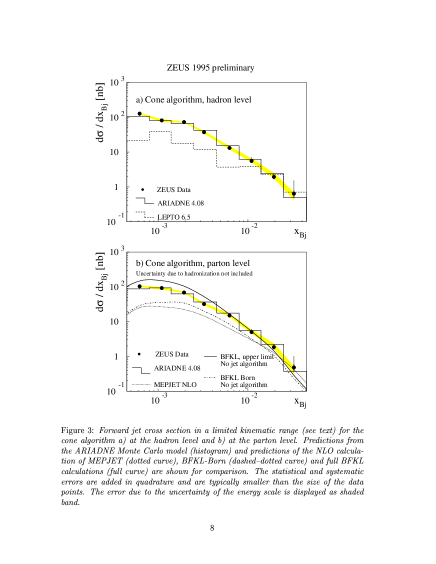
8.5 Summary and Outlook
The hadronic final state has been searched for an unsuppressed parton radiation pattern, which could for example be expected from BFKL contributions, in contrast to pure DGLAP evolution. The high level of transverse energy is consistently described when BFKL evolution is included, but possibly large hadronization effects could also mimick the effect. In order to describe the data with DGLAP evolution, hadronization phenomenology has introduced new concepts like soft colour interactions in LEPTO, or it involuntarily produces “not exponentially suppressed rapidity gaps” by cluster fragmentation in HERWIG.
The forward jet measurements at low are in rough agreement with BFKL expectations, but are also plagued by hadronization uncertainties. With larger statistics data sample, the measurements could be made at higher where a closer relation between hadron jets and partons is expected [294]. From the measured flows and forward jets, a suppressed radiation scenario is presently only tenable when large hadronization effects are assumed.
The measured single particle spectra require more parton radiation than is expected from pure DGLAP evolution, regardless of the hadronziation model. The spectra have been calculated via known fragmentation functions in the DGLAP and the BFKL scheme. In the DGLAP scenario the calculation by far underestimates the data.
Whereas pure DGLAP evolution fails, BFKL evolution offers a plausible explanation of the measurements. This does of course not preclude other explanations. For example, it has been suggested that contributions from resolved photons, where the hard interaction happens not at the photon vertex but further down the ladder, could be responsible for the additional parton activity [255, 297]. We have seen possible signs for such effects also in the inclusive jet rates, see section 7.6. More refined measurements to unravel the details of parton dynamics at low , including correlations between jets and hadrons, have been proposed [58, 263]. It will also be important to check the consistency of the competing models by confronting them with the entire data on the hadronic final state.
BFKL effects are also being looked for in collisions at the Tevatron. A jet-jet decorrelation is seen with increasing rapidity difference, though the effect is larger than expected from BFKL, and is described by the HERWIG and PYTHIA models without BFKL dynamics [298]. Recently, BFKL effects have been brought forward to explain the discrepancy between measured jet rates and NLO calculations at small jet transverse energies for different CM energies at the Tevatron [299].
Chapter 9 Instantons
9.1 Introduction
For a long time it has been recognized that the standard model contains processes which cannot be described by perturbation theory, and which violate classical conservation laws like baryon number () and lepton number () in the case of the electroweak interaction, and chirality () in the case of the strong interaction [300]. Such anomalous processes are induced by so-called instantons [301]. The name indicates that these are non-perturbative fluctuations that are confined to “an instant” in space-time, with no corresponding free particle solutions for . The interest in instantons remained somewhat academic, as observable effects were predicted to exist only at extremely high energies of , until it was discovered that their exponential suppression is much reduced by the emission of gauge bosons [302]. In electroweak theory with massive gauge bosons still rather high energies of would be required, but not so in QCD with massless gluons and strong coupling. Instanton effects could play a rôle in QCD reactions already at present day colliders. Deep inelastic scattering at HERA is particularly interesting, because the virtuality of the photon probe provides a hard scale for the instanton subprocess, which is needed for theoretically sound predictions [303, 304, 305]. Instanton effects have not yet been observed in nature. Their experimental discovery would be of fundamental significance for particle physics.
Here a short introduction to the basic theoretical ideas will be given (a pedagogical treatment of instantons can be found in [306]). Instanton phenomenology in deep inelastic scattering (DIS) will be discussed, covering cross sections and event topologies. Finally, prospects for instanton searches and first results from the analysis of HERA data will be presented.
9.2 Instanton Theory
Instantons originate from the non-trivial topological structure of the vacuum in non-Abelian gauge field theories, where the vacuum is degenerate in the Chern-Simons number . is defined as an integral over the gauge fields with coupling ,
| (9.1) |
![[Uncaptioned image]](/html/hep-ph/9712505/assets/x119.png)
Fig. 9.1. The structure of the vacuum. Instanton solutions represent tunnelling transitions between topological inequivalent minima, which cannot be reached perturbatively.
Neighbouring vacua have the same (minimal) potential energy, but differ in their topological winding number , and are separated by a potential barrier of height (fig. 9.2). The usual perturbative expansion of the scattering amplitudes in the coupling constant around one minimum (fig. 9.2), conveniently represented by a series of Feynman graphs, does not allow for transitions between neighbouring minima. They may however occur classically when the energy is large enough , or by quantum mechanical tunnelling when , corresponding to so-called instanton solutions of the classical field equations. The transition amplitude for the instanton–induced tunnelling process is exponentially suppressed , a very small number.


In the electroweak theory, the minimal barrier height is . Instanton transitions between vacua separated by (see fig. 9.2a for an example) would violate baryon () and lepton numbers () according to
| (9.2) |
but respect
| (9.3) |
is the number of fermion generations.
In instanton induced QCD reactions (see fig. 9.2b) chirality is violated. The chirality is the difference between the number of left- and right-handed fermions, . For active quark flavours, the selection rule is
| (9.4) |
The minimal barrier height is given by the hard scale of the process, e.g. for DIS [304]. The exponential suppression is less severe than in the electroweak case, because .
9.3 Instantons at HERA
In recent years, it has been realized [304, 305, 307, 308, 309, 310] that quantitative calculations are possible for processes induced by QCD instantons in DIS due to the presence of a hard scale, . In DIS, events due to QCD instantons (and anti-instantons ) are predominantly produced in a photon-gluon fusion processes111Quark initiated processes have not yet been considered. Due to the large gluon content of the proton in the HERA domain at small , they are expected to be of minor importance. In addition, they are expected to be suppressed by with respect to the gluon initiated processes. (Fig. 9.3)
| (9.5) |
In each event, quarks and antiquarks of all active flavours are found, with gluons in addition.
 |
|
The kinematics is depicted in fig. 9.3. The DIS variables Bjorken and can be measured from the scattered electron, . A measurement of the other variables is more challenging. A measurement of the invariant mass of the hadronic system, excluding the remnant, would determine . If the outgoing “current jet” could be identified and measured, it’s 4-momentum would determine , and thus the variables and which characterise the instanton subprocess. In practice, when not all of the five independent invariants (for example ) can be measured, they are being integrated over.
The instanton induced cross section is given by a convolution of the probability to find a gluon in the proton , the probability that the virtual photon splits into a quark-antiquark pair in the instanton background , and the cross section of the instanton subprocess [305, 307]. Multi-gluon emission enhances the cross section [302]
| (9.6) |
The cross section of the instanton induced subprocess is then [305]:
| (9.7) |
It depends critically on the functions (called the “holy grail” function), which modifies the exponent in the suppression factor , and on , which depends on . There exists also a scale dependence due to the choice of the renormalization scale .
![[Uncaptioned image]](/html/hep-ph/9712505/assets/x123.png)
Fig. 9.4. The holy grail function [305]. For small (), instanton perturbation theory is applied. The calculation with the valley method matches smoothly with the perturbative result.
can be estimated reasonably well (see fig. 9.3) for not too small, [305]. The extrapolation to lower values of is unreliable due to inherent ambiguities. In addition, multi-instanton effects should be avoided by limiting the instanton size (the spatial region occupied during the interaction) to with a cut-off [305, 307]. That requirement ensures also that stays small enough to apply instanton perturbation theory.
The resulting instanton induced subprocess cross section (see fig. 9.5) is peaked at and exponentially grows with decreasing . The integrated instanton induced DIS cross section (see fig. 9.6) is sizeable; for and it is of . The cross section is approximately scaling (depends only on , not on for large ) [307]. It grows towards small , and increases dramatically when the lower cut-off is relaxed. Eventually higher order instanton effects have to dampen the growth of the cross section.
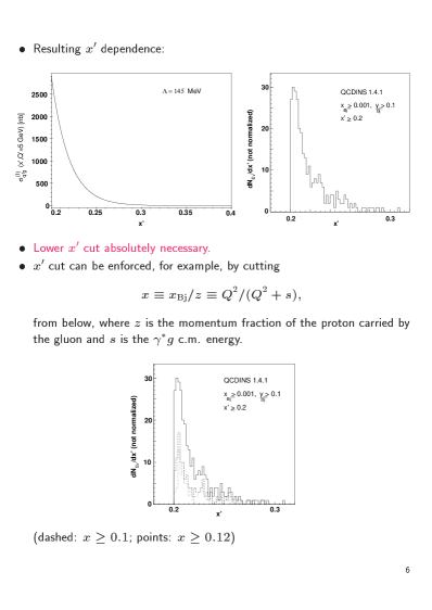
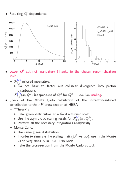
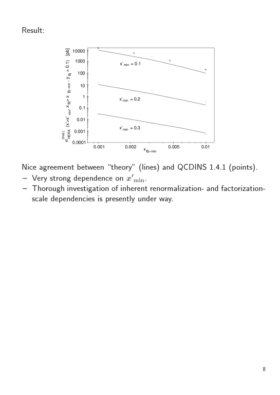
Two kinematic regions have to be distinguished. For the predictions are relatively safe, allowing the instanton theory to be tested. Either instantons are discovered at the predicted level – including the substantial theoretical uncertainties, which still need to be quantified –, or the theory has to be revised. For the cross section presumably continues to grow, but the extrapolation is extremely uncertain. For a discovery, this is the favourable region due to the large cross section. A negative result however cannot be turned against the theory, it would rather restrict the unknown behaviour of at small . Most promising is the kinematic region of small Bjorken-, because both the total DIS cross section and the predicted fraction of instanton induced events increase towards small (see fig. 9.9b).
9.4 Experimental Signatures
In the theoretically safe region, , the expected fraction of instanton events in all DIS events is of (compare fig.9.9b), too small to be detected in inclusive cross section measurements (i.e. the structure function ). Instead, dedicated searches for the characteristic features of instanton events in the hadronic final state have to be performed. A Monte Carlo generator (QCDINS [311]) to simulate the hadronic final state of instanton events in DIS is available. In general, the event shape predictions are more stable than the rate predictions, because poorly known factors cancel. The instanton event properties can be contrasted with predictions from event generators for normal DIS events (ARIADNE [86], LEPTO [81] and HERWIG [82]) which give an overall satisfactory description of the DIS final state properties [123].
In the rest frame quark and antiquarks and gluons are emitted isotropically from the instanton subprocess. is Poisson distributed with [307, 309]
| (9.8) |
After hadronization, this leads to a spherical system with a high multiplicity of hadrons, depending mainly on the available centre of mass energy . For a typical situation (), . About partons and hadrons are expected. The expected parton momentum spectrum is semi-hard [304] with transverse momentum .
Hadronic final state properties are conveniently being studied in the centre of mass system (CMS) of the incoming proton and the virtual boson, i.e. the CMS of the hadronic final state. Longitudinal and transverse quantities are calculated with respect to the virtual boson direction (defining the direction). The pseudorapidity is defined as , where is the angle with respect to the virtual photon direction. When boosted to the CMS, the hadrons emerging from the instanton subprocess occupy a band in pseudorapidity of half width , which is homogeneously populated in azimuth [304].
The characteristics of instanton events by which they can be distinguished from normal DIS events are therefore: high multiplicity with large transverse energy; spherical event configuration (apart from the current jet); and the presence of all flavours (twice!) that are kinematically allowed in each event. One would therefore look for events which in addition to the other characteristics are rich in s, charm decays, secondary vertices, muons etc.. In general, the strength of instanton signals in the hadronic final state increases somewhat towards low and large due to the increasing “instanton mass” .


The “instanton band” shows up in the flow of hadronic transverse energy as a function of (fig. 9.7a). It’s height and position depends on and (and also on and ). In normal DIS events on average an of per unit is observed. In instanton induced events, that number may go up to GeV for low . A possible search strategy could involve the distribution in a selected rapidity band (fig. 9.7b), looking for high events in the tail of the distribution [313, 312].
Further discrimination can be obtained [313] from the fact that for instanton events the should be distributed isotropically, while normal DIS events are jet-like, in particular for large . One defines
| (9.9) |
The sum runs over all final state hadrons with momentum . is the unit vector perpendicular to the virtual photon axis which minimizes and thus defines the event plane. lies in the event plane and is normal to both and the virtual photon axis. It is easy to show that for an ideal isotropic “instanton decay”, [313]. The “instanton mass” can thus be reconstructed experimentally (fig. 9.8a). Normal DIS events, either “1+1” or “2+1” jet events (the +1 refers to the unobserved proton remnant) are contained in the event plane, , in contrast to instanton events with (see fig. 9.8b).
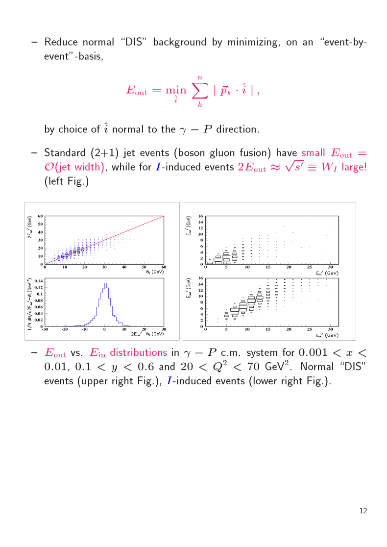
Instanton events are characterized by a large particle density localized in rapidity. In normal DIS events there are about 2 charged particles per unit of pseudorapidity [118], rather uniformly distributed in . For a low cut-off, that number goes up to 10 in the peak of the instanton band [312]. Very sensitive to instanton events is the charged particle multiplicity distribution [312], see fig. 9.9a. A significant fraction of the instanton events would lead to charged multiplicities which are very unlikely to be found in normal DIS events. Furthermore, particle-particle correlation functions should be influenced by instanton effects [314].


9.5 Searches for Instanton Processes
The fact that instanton events look very different from the expectation for standard QCD events can be exploited to search for instanton signals in the HERA data. One strategy is to compare the shape of hadronic final state distributions to the expectation from standard QCD events (nDIS) with an admixture of instanton events (INSDIS) of fraction . In case the measured distribution agrees with the standard QCD expectation, a limit on the fraction of instanton induced events in DIS can be set. The caveat of this method is that one has to make an assumption on what standard QCD looks like. In particular at small that issue is under debate [278, 246, 315], see section 7.6 and chapter 8. There exists a danger that an instanton effect is tuned or explained away by stretching the standard QCD predictions by generator tuning, introducing BFKL effects etc.. A good understanding of standard QCD will therefore be crucial for the positive identification of instanton effects.
In the first search for instanton events [117] an anomalous yield has been looked for. For about 0.12 mesons (including ) have been measured per event and unit pseudorapidity, with a relatively flat distribution. For instanton events with , a peaked distribution with about 0.55 per event and unit is expected. From the comparison with standard QCD event generators [86, 81, 82] and the instanton generator [311] an upper limit of at 95% C.L. is obtained [117].
The charged particle multiplicity distribution in high energy reactions can often by described by a negative binomial distribution (NBD). Also the DIS data are relatively well described by NBDs [116]. The multiplicity distribution from the CMS interval for events with (corresponding to ) can be parametrized with an NBD of mean . Possible deviations from an NBD allow for an instanton fraction of at most =2.7% at 95% C.L. [116].
Other measured event shapes have been systematically analysed in terms of their sensitivity to instanton events [312], and their dependence on the kinematic variables . The most sensitive distributions were the transverse energy flows [114], the pseudorapidity distribution of charged particles and their spectra [118]. For example, the flow has been measured over a wide range of and , allowing to extend the search region down to . From a shape analysis [312] (see fig. 9.7), instanton fractions between 5 and 13 % can be excluded for (see figs. 9.9b, 9.10). For lower the signal is more prominent, and somewhat better limits are obtained.
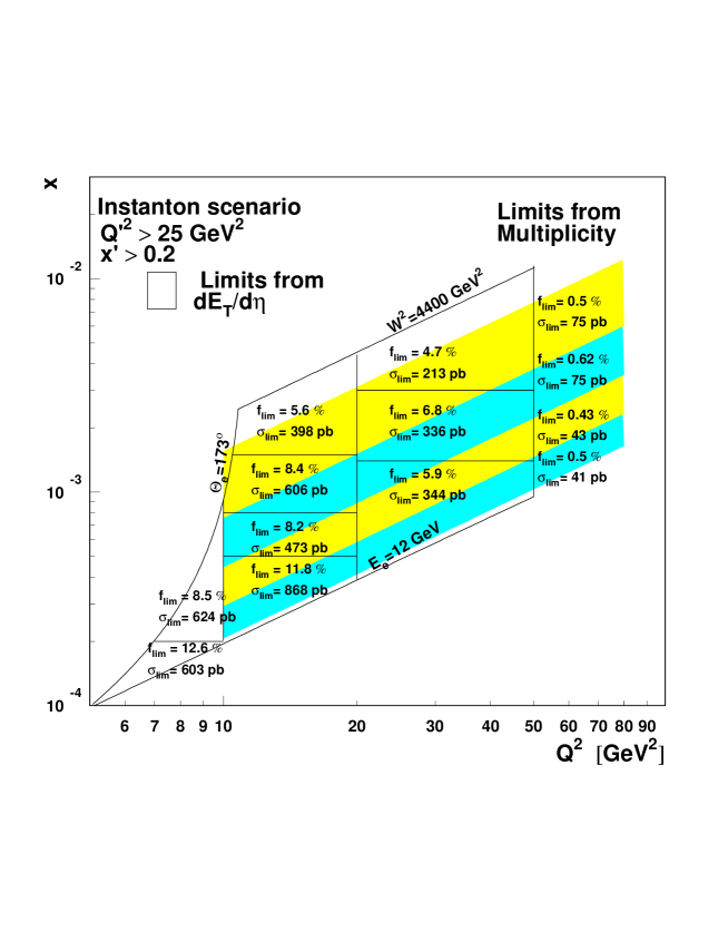
The fact that H1 [116] did not observe any events above a certain multiplicity has been exploited [312] to place more stringent limits on instanton production222The previous limits from the H1 multiplicity analysis [116] were derived from the shape of the multiplicity distribution for .. A significant fraction of instanton induced events would have multiplicities (compare fig. 9.9a). Instanton fractions can therefore be excluded for (see figs. 9.9b, 9.10), and somewhat lower values for a lower cut-off [312]. This search method has the advantage that, in contrast to the previous shape comparisons, it does not rely on assumptions for standard QCD event topologies, since no background needs to be subtracted. Unavoidable of course is the dependence on the expected instanton event shape, which may be even more uncertain than the standard QCD event shapes.
| analysis | DIS kinematics covered | instanton scenario | limit | |||
|---|---|---|---|---|---|---|
| () | (GeV) | () | ||||
| [117] | 10 – 70 | 0.001 – 0.01 | 95 – 230 | 6 % | ||
| multipl. [116] | 10 – 80 | 0.0007 – 0.012 | 80 – 115 | 2.7 % | ||
| flows [312] | 5 – 50 | 0.0001 – 0.01 | 65 – 230 | 5 – 13 % | ||
| multipl. [312] | 10 – 80 | 0.0001 – 0.01 | 80 – 220 | 0.4 – 0.6 % | ||
The available bounds on instanton production are summarised in tab. 9.1. The most stringent limits for the theoretically “safe” scenario are still a factor 20 higher than what is predicted from the instanton theory, see fig. 9.9b. Limits for other scenarios can be found in [312]. For they are already below the naive extrapolation into the theoretically uncertain region, providing a constraint for the theory and the holy grail function .
9.6 Conclusion
Instanton transitions, a yet unexplored facette of non-abelian gauge field theories, have been discussed. While in the electroweak theory the violating effects induced by instantons are expected only at energies , their chirality violating pendant in QCD could lead to striking signatures already at present day colliders. In DIS at HERA, these are a high particle multiplicity with large transverse energy localized in rapidity, and , and possibly quarks in the final state.
The expected contribution to DIS events from instantons is of , with substantial theoretical uncertainties. First analysis of HERA data taken in the years , corresponding to an integrated luminosity of , are still a factor above the prediction. With higher statistics data samples ( up to the end of 1997) and improved search strategies, a fundamental discovery at HERA appears to be in reach.
As the study of the hadronic final state at HERA has shown, model predictions for normal DIS final states are not unique. It will probably be safe to take some uncertainty into account also for the prediction of the instanton final state. A good understanding of QCD in DIS will be vital for instanton searches.
It might be possible to exploit also other reactions than DIS, such as photoproduction, where the hard scale needed for reliable instanton calculations could be provided by the of a jet. Instantons have even be proposed [316] as an explanation of the possible excess of high events at HERA [43, 44, 45].
Chapter 10 Summary
HERA has entered a new kinematic regime in deep inelastic scattering: at small , large and both small and large . After five years of HERA operation, the hadronic final state has been measured in great detail. The large body of data has been confronted with QCD, the theory of the strong interaction.
We have seen progress happening at different stages:
-
•
QCD predictions are tested experimentally, and parameters of the theory are being extracted. An example are the measurements of jet rates and the extraction of or of the gluon density in the proton.
-
•
Where the theory is less well established, there is an interplay between experimental data and theory, in which new ideas are born and developed (or rejected). Examples are soft colour interactions as an explanation for rapidity gaps and large flows, or power corrections for hadronization effects.
-
•
The data are not yet understood. Either there exist no predictions, or there are conflicting explanations. An example are the measured forward jet rates, which could be explained by BFKL evolution, or by hadronziation effects, or by a resolved structure of the virtual photon.
The availability of as much data as possible over a wide kinematic range is very important for the scientific process to work efficiently. A new idea which explains one aspect of the data can be rejected early if it fails in another. The data have severely constrained QCD models for the hadronic final state which varied widely before the data had become available.
General event properties in deep inelastic scattering at HERA
In the hadronic CMS, the produced hadrons cover about 5 units of rapidity in either hemisphere, depending mainly on the available CM energy of the hadronic system, . There are about 2.5 charged particles per unit rapidity, and the transverse energy is on average 2 GeV per unit rapidity. Multiplicity distributions exhibit the familiar KNO scaling, and Bose-Einstein correlations are measured similar to other reactions. A large rapidity gap is found in about 10% of the events. Around 25% of the events contain charm. In the current hemisphere about 0.9 mesons and 0.15 particles are measured per event. In 5 to 10% of the events more than one jet is found (apart from the remnant).
The global event features are largely determined by the available phase space given by the CM energy of the hadronic system. The dependence on the photon virtuality has also been studied. In the current region the transverse activity (flow, spectra, jets) increases with . In the central rapidity region dependencies are small. Here the data are similar to what has been measured in photoproduction (=0) or hadron-hadron collisions. The particle density per unit rapidity increases slower than in annihilation with the available CM energy . When compared with DIS data at lower , a faster than logarithmic rise of the average multiplicity is observed.
Comparisons with QCD
Transverse energy and momentum distributions provide evidence for hard QCD radiation beyond the LO matrix element. More has been measured than anticipated before HERA data taking. It is not yet clear whether soft colour interactions are required to describe the transverse energy flow, or whether not yet well established perturbative QCD effects are responsible for the large measured. Soft colour interactions are of interest also because they provide a mechanism for producing rapidity gaps. Alternatively, colour dipole radiation or BFKL evolution can be employed to produce as much as seen in the data.
The scaled charged particle momentum spectra measured either in the current hemispheres of the hadronic CMS with as scale or the Breit frame with as scale are in general well described by QCD models in various approximations of the perturbative shower evolution in conjunction with non-perturbative hadronization models. Where applicable, perturbative QCD calculations in NLO employing fragmentation functions measured elsewhere are in agreement with the data. Scaling violations of the spectra will provide a means to measure .
The growth of multiplicity with energy is described by perturbative QCD calculations in the MLLA approximation, assuming local parton hadron duality (LPHD). The shape of the momentum spectra in the “hump backed” form is approximately Gaussian. It’s evolution with is consistent with the MLLA+LPHD expectation assuming soft colour coherence. Models without soft colour coherence describe the data less well. When allowance is made for the boson-gluon fusion process in DIS, the particle spectra are similar to what has been measured in annihilation. Evidence is found for the prediction that the soft part of the Lorentz invariant spectrum is independent of the energy of the fragmenting parton. The assumption of a constant coupling is in stark conflict with the data.
Global event shape variables like thrust, jet mass and jet broadening in the Breit frame current hemisphere show an increasing event collimation with energy . “Power corrections” supplementing the NLO calculations provide a good description of the data. The power corrections parametrize higher orders and hadronization effects and appear to be universal within 20% – the same normalization parameter can be used for different shape variables and as well as reactions. The concept of “power corrections” may turn out to be very fruitful for the understanding of hadronization effects. Assuming power corrections, the strong coupling has been determined with competitive precision.
Of similar precision is the determination from the rate of 2+1 jet events. The strong coupling has been measured as a function of from 2+1 jet events in a region where NLO QCD is able to describe the data, namely where is not too small. The data are consistent with the expected dependence of the running coupling. However, the optimal strategy for measurements from jets has not yet been found. A better understanding of the connection between measured hadron jets and perturbative QCD predictions for parton jets appears to be needed. Smaller theoretical uncertainties are anticipated with other jet algorithms and increased statistics at higher or jet .
At small and and in particular towards the proton remnant the measured jet rates are larger than expected from either NLO calculations or conventional QCD models. “Conventional” stands for deep inelastic scattering, where a virtual photon scatters on a parton in a proton, and where the partons in the proton obey DGLAP evolution with as scale. A good description is obtained either by the colour dipole model, or by a model in which the partonic content of the virtual photon is resolved by the large jet .
A strong growth of the gluon density towards small has been inferred from DGLAP analyses of structure function measurements. This is confirmed by direct measurements from jet and charm production, by which photon-gluon fusion processes can be tagged. The errors are still large, however. It will be very important to extend such direct measurements towards smaller values.
Small physics has received considerable interest. It has been speculated that the rise of with decreasing is a sign for BFKL evolution, but DGLAP evolution was found to be able to account for the data as well. Traces of BFKL evolution have therefore been searched for in less inclusive observables in the hadronic final state, namely enhanced transverse activity in between the current and the target fragmentation regions: transverse energy flow, high particles, “forward jets”. The data could not be described by conventional DGLAP evolution. Though BFKL calculations can explain the measured enhanced activity, there exist competing explanations, again making use of a virtual photon structure. It remains to be seen though whether or not such an alternative model would be in conflict with other HERA data. In case both explanations work equally well, one might speculate that they have more in common than is apparent.
Finally, the possibility exists to discover QCD instanton effects at HERA. Such a discovery would open a new field of non-perturbative QCD, and would imply also baryon and lepton number violation in the electroweak sector already within the standard model. Observable effects are predicted for the hadronic final state, and first bounds on instanton production have been placed. The predicted cross sections are such that it appears likely that with increased sensitivity instantons can be discovered at HERA, or the theory in its present form can be rejected.
Acknowledgements
This work has been made possible by a grant from the Deutsche Forschungsgemeinschaft. I would like to thank G. Buschhorn from the Max-Planck-Institut für Physik in Munich for the hospitality I have experienced in his group during the last two years. I have enjoyed very much the close collaboration in the MPI group, in particular with F. Botterweck, T. Carli and G. Grindhammer.
I wish to thank all my colleagues from the H1 and ZEUS experiments on whose research this work is based for their collaboration and friendly competition at HERA. I would like to thank J. Dainton, E. Lohrmann, B. Naroska and A. Wagner for their continuous encouragement and their support to undertake the Habilitation and to teach at the Universität Hamburg.
I am grateful to J. Bartels, E. De Wolf, A. Martin, G. Ingelman, A. Ringwald and F. Schrempp for their patient explanations of sometimes heavy theory, and for enlightening discussions, in which some very fruitful ideas were born. Helpful discussions with B. Andersson, Y. Dokshitzer, D. Graudenz, L. Lönnblad, M. Seymour, S. Lang, E. Mirkes and B. Webber are gratefully acknowledged.
Finally, I would like to thank J. Bartels, N. Brook, T. Carli, T. Doyle, A. De Roeck, E. De Wolf, G. Grindhammer, J. Hartmann, G. Ingelman, H. Jung, A. Levy, E. Lohrmann, U. Martyn, D. Milstead, B. Naroska, N. Pavel, J. Repond, A. Ringwald, F. Schrempp, F. Sefkow and V. Shekelyan for their comments on the manuscript, or parts of it. Their critical reading has been invaluable.
Bibliography
- [1] A. Levy, DESY 97-013, Lectures given at “Strong Interaction Study Days”, Kloster Banz, 1995.
- [2] B. Badelek and J. Kwieciński, Rev. Mod. Phys. 68 (1996) 445.
-
[3]
N. Cartiglia, hep-ph/9703245, Proc. SLAC summer school 1996;
P. Newman, hep-ex/9707020, to appear in Proc. Workshop DIS97, Chicago 1997, eds. J. Repond and D. Krakauer;
E. Gallo, hep-ex/9710013, to appear in Proc. Lepton-Photon Conf., Hamburg 1997. - [4] M. Erdmann, The Partonic Structure of the Photon, Springer Verlag 1997.
- [5] N. Schmitz, Int. J. Mod. Phys. A3 (1988) 1997; MPI-PhE/92-23, Proc. XXII Intern. Symp. on Multiparticle Dynamics, Santiago de Compostela 1992.
- [6] H1 Collab., I. Abt et al., Nucl. Instr. and Meth. A386 (1997)310 .
- [7] H1 Collab., I. Abt et al., Nucl. Instr. and Meth. A386 (1997)348 .
-
[8]
ZEUS Collab., M. Derrick et al., Phys. Lett. B293 (1992) 465, Z. Phys. C63
(1994) 391;
A. Caldwell, Proc. ICHEP 92, Dallas 1992, ed. J. R. Sanford, vol. II, p. 1856. - [9] F. Jacquet, A. Blondel, in Proc. of the study of an facility for Europe, ed. U. Amaldi (1979), p. 391.
- [10] U. Bassler and G. Bernardi, Nucl. Instr. Meth. A361 (1995) 118.
- [11] L.N. Hand, Phys. Rev. 129 (1963) 1834.
- [12] J. Bartels and C. Bontus, to appear in Proc. Workshop DIS97, Chicago 1997, eds. J. Repond and D. Krakauer.
- [13] R. G. Roberts, The structure of the proton, Cambridge University Press, 1990.
- [14] R.M. Barnett et al, Particle Data Group, Review of Particle Physics, Phys. Rev. D54 (1996) no. 1.
-
[15]
Yu. L. Dokshitzer, Sov. Phys. JETP 46 (1977) 641;
V.N. Gribov and L.N. Lipatov, Sov. J. Nucl. Phys. 15 (1972) 438 and 675;
G. Altarelli and G. Parisi, Nucl. Phys. 126 (1977) 297 . - [16] A. Martin, Durham preprint DTP/93/66, lectures given at XXI Intern. Meeting on Fundamental Physics, Miraflores de la Sierra 1993.
-
[17]
A. DeRujula et al., Phys. Rev. D10 (1974) 1649
B. Badelek et al., J. Phys. G.: Nucl. Part. Phys. 22 (1996) 815. -
[18]
E.A. Kuraev, L.N. Lipatov and V.S. Fadin, Sov. Phys. JETP 45 (1972) 199;
Y.Y. Balitsky and L.N. Lipatov, Sov. J. Nucl. Phys. 28 (1978) 282. - [19] M. Ciafaloni, hep-ph/9709390, to appear in Proc. Workshop “New Trends in HERA Physics”, Schloß Ringberg, Tegernsee 1997.
-
[20]
M. Ciafaloni, Nucl. Phys. B296 (1987) 249;
S. Catani, F. Fiorani and G. Marchesini, Phys. Lett. B234 (1990) 339, Nucl. Phys. B336 (1990) 18. - [21] A.D. Martin, Proc. Workshop DIS96 on “Deep Inelastic Scattering and Related Phenomena”, Rome 1996, eds. G. D’Agostini and A. Nigro, p. 156.
-
[22]
G. Salam, hep-ph/9707382, to appear in Proc.
Workshop “New Trends in HERA Physics”,
Schloß Ringberg, Tegernsee 1997;
M. Scorletti, hep-ph/9710559, to appear in Proc. Madrid Workshop on “Low Physics”, Miraflores de la Sierra 1997. - [23] B. Andersson G. Gustafson and H. Kharraziha, LU-TP 97-29.
-
[24]
B. Andersson, G. Gustafson and J. Samuelsson, Nucl. Phys. B463 (1996) 217;
B. Andersson, G. Gustafson H. Kharraziha and J. Samuelsson, Z. Phys. C71 (1996) 613. - [25] P. Landshoff, hep-ph/9410250, Proc. “Hadronic Aspects of Collider Physics”, Zuoz 1994.
- [26] P. D. B. Collins and A. D. Martin, Hadron Interactions, Adam Hilger Ltd., Bristol 1984.
- [27] J. R. Forshaw and D. A. Ross, Quantum Chromodynamics and the Pomeron, Cambridge University Press, 1997.
- [28] P. D. B. Collins, An Introduction to Regge Theory & High Energy Physics, Cambridge University Press, 1977.
- [29] WA91 Collab., S. Albatzis et al., Phys. Lett. B321 (1994) 509.
- [30] A. Donnachie and P.V. Landshoff, Phys. Lett. B296 (1992) 227.
- [31] S. Levonian, hep-ph/9612206, Proc. ICHEP 96, Warsaw 1996, p. 17.
-
[32]
M. Froissart, Phys. Rev. 123 (1961) 1053;
A. Martin, Nuovo Cimento 42 (1966) 930. - [33] ZEUS Collab., M. Derrick et al., Phys. Lett. B316 (1993) 412; Z. Phys. C65 (1995) 379.
- [34] ZEUS Collab., M. Derrick et al., Z. Phys. C69 (1996) 607; Z. Phys. C72 (1996) 399.
- [35] ZEUS Collab., J. Breitweg et al., Phys. Lett. B407 (1997) 432.
- [36] B. Surrow for the ZEUS Collab., to appear in Proc. Workshop DIS97, Chicago 1997, eds. J. Repond and D. Krakauer.
- [37] H1 Collab., I. Abt et al., Nucl. Phys. B407 (1993) 515 .
- [38] H1 Collab., T. Ahmed et al., Nucl. Phys. B439 (1995) 471.
- [39] H1 Collab., S. Aid et al., Nucl.Phys. B470 (1996) 3.
- [40] H1 Collab., C. Adloff et al., Nucl. Phys. B497 (1997) 3 .
- [41] H1 Collab., contrib. paper 260 to HEP97, Jerusalem 1997.
- [42] H1 Collab., C. Adloff et al., Phys. Lett. B393 (1997) 452.
- [43] H1 Collab., C. Adloff et al., Z. Phys. C74 (1997) 191.
- [44] ZEUS Collab., J. Breitweg et al., Z. Phys. C74 (1997) 207.
-
[45]
B. Straub for the H1 and ZEUS Collab., Lepton-Photon Conference, Hamburg
1997;
E. Elsen for the H1 and ZEUS Collab., EPS-HEP97 Conference, Jerusalem 1997. - [46] E665 Collab., M.R. Adams et al., Phys. Rev. D54 (1996) 3006.
- [47] NMC Collab., M. Arneodo et al., Phys. Lett. B364 (1995) 107.
- [48] BCDMS Collab., A.C. Benvenuti et al., Phys. Lett. B223 (1989) 485; CERN-EP/89-06.
- [49] M. Glück, E. Reya, A. Vogt, Z. Phys. C67 (1995) 433; C53 (1992) 127; C48 (1990) 471.
- [50] R.D. Ball and S. Forte, Phys. Lett. B335 (1994) 77, ibid. B336 (1994) 77.
- [51] J. Kwieciński, A.D. Martin and A. M. Stasto, Phys. Rev. D56 (1997) 3991.
- [52] K. Prytz, Phys. Lett. B311 (1993) 286.
- [53] R. Devenish, to appear in Proc. Lepton-Photon Conf., Hamburg 1997.
- [54] M. A. J. Botje, NIKHEF-97-028, to appear in Proc. Workshop DIS97, Chicago 1997, eds. J. Repond and D. Krakauer.
- [55] NMC Collab., M. Arneodo et al., Phys. Lett. B309 (1993) 222.
- [56] A.D. Martin, R.G. Roberts and W.J. Stirling, Phys.Lett.B387 (1996) 419.
- [57] H.L. Lai et al., Phys. Rev. D55 (1997) 1280.
- [58] K. Charchula and E.M. Levin, Proc. Workshop on “Physics at HERA”, Hamburg 1991, eds. W. Buchmüller and G. Ingelman, vol. 1, p. 223.
- [59] A.H. Mueller, J. Phys. G, Nucl. Par. Phys. 19 (1993) 1463.
- [60] A.H. Mueller and H. Navelet, Nucl. Phys. B282 (1987) 727.
- [61] R.D. Ball and S. Forte, Phys. Lett. B358 (1995) 365.
- [62] M. A. J. Botje, NIKHEF-97-029, to appear in Proc. Workshop DIS97, Chicago 1997, eds. J. Repond and D. Krakauer.
-
[63]
A. Zee, F. Wilczek and S.B. Treiman, Phys. Rev. D10 (1974) 2881;
G. Altarelli and G. Martinelli, Phys. Lett. B76 (1978) 89. - [64] A.M. Cooper-Sarkar et al. , Z. Phys. C39 (1988) 281.
-
[65]
A. M. Cooper-Sarkar, R. C. E. Devenish and M. Lancaster, Proc. Workshop on
“Physics at HERA”, Hamburg 1991, eds.
W. Buchmüller and G. Ingelman, vol.
1, p. 155;
M. W. Krasny, W. Placzek and H. Spiesberger, Proc. Workshop on “Physics at HERA”, Hamburg 1991, eds. W. Buchmüller and G. Ingelman, vol. 1, p. 171;
L. Bauerdick, A. Glazov and M. Klein, Proc. Workshop on “Future Physics at HERA”, Hamburg 1995-1996, eds. A. De Roeck, G. Ingelman and R. Klanner, vol. 1, p. 77. - [66] H1 Collab., S. Aid et al., Z. Phys. C69 (1995) 27.
- [67] ZEUS Collab., M. Derrick et al., Z. Phys. C63 (1994) 391.
-
[68]
D.O. Caldwell et al., Phys. Rev. Lett. 40 (1978) 1222;
S.I. Alekhin et al., CERN-HERA 87-01 (1987). - [69] A. Donnachie and P.V. Landshoff, Z. Phys. C61 (1994) 139.
- [70] A pedagogical presentation is in J. Collins, hep-ph/9705393.
- [71] R.P. Feynman, Phys. Rev. Lett. 23 (1969) 1415.
- [72] R.P. Feynman and R.D. Field, Phys. Rev. D15 (1977) 2590; Nucl. Phys. 136B (1978) 1.
- [73] B.R. Webber, J. Phys. G17 (1991) 1579.
- [74] T. Sjöstrand, CERN-TH/95-10, Proc. XV Brazilian National Meeting on Particles and Fields, Angra dos Reis, 1994.
- [75] B. R. Webber, Cavendish-HEP-94/17, Proc. “Hadronic Aspects of Collider Physics”, Zuoz 1994.
- [76] Proc. HERA workshop, Eds. W. Buchmüller and G. Ingelman, Hamburg (1991) Vol. 3 .
-
[77]
G. Altarelli and G. Martinelli, Phys. Lett. B76 (1978) 89;
R. Peccei and R. Rückl, Nucl. Phys. B162 (1980) 125;
A. Méndez, Nucl. Phys. B145 (1978) 199;
C. Rumpf, G. Kramer and J. Willrodt, Z. Phys. C7 (1981) 337;
J. G. Körner, E. Mirkes and G. A. Schuler, Int. J. Mod. Phys. A4 (1989) 1781. - [78] S. Catani, M. Seymour, Phys. Lett. B378 (1996) 287 , Nucl. Phys. B485 (1997) 291.
-
[79]
E. Mirkes and D. Zeppenfeld, Phys. Lett. B380 (1996) 105; Acta Phys. Pol. B27
(1996) 1393;
E. Mirkes, hep-ph/9711224, Habilitationsschrift Univ. Karlsruhe. - [80] D. Graudenz, DISASTER++ 1.0 manual, hep-ph/9710244.
-
[81]
G. Ingelman, Proc. Workshop on
“Physics at HERA”, Hamburg 1991, eds.
W. Buchmüller and G. Ingelman, vol. 3, p. 1366;
G. Ingelman, A. Edin and J. Rathsman, Comp. Phys. Comm. 101 (1997) 108. - [82] G. Marchesini et al., Comp. Phys. Comm. 67 (1992) 465 .
- [83] H. Jung, Comp. Phys. Comm. 86 (1995) 147.
-
[84]
G. Gustafson, Ulf Petterson, Nucl. Phys. B306 (1988);
G. Gustafson, Phys. Lett. B175 (1986) 453;
B. Andersson, G. Gustafson, L. Lönnblad, Ulf Petterson, Z. Phys. C43 (1989) 625 . - [85] F. Halzen and A. D. Martin, Quarks and Leptons, John Wiley & Sons, 1984.
- [86] L. Lönnblad, Comp. Phys. Comm. 71 (1992) 15.
-
[87]
L. Lönnblad, Z. Phys. C65 (1995) 285; CERN-TH/95-95;
A. H. Mueller, Nucl. Phys. B415 (1994) 373 . - [88] J. Rathsman, Phys. Lett. B393 (1997) 181.
- [89] H. Kharraziha and L. Lönnblad, LU-TP 97-21, hep-ph/9709424.
- [90] Yu. L. Dokshitzer, V. A. Khoze, A. H. Mueller and S. I. Troyan, Basics of Perturbative QCD, Editions Frontières, 1991.
-
[91]
T. Sjöstrand, Comp. Phys. Comm. 39 (1986) 347, CERN-TH-6488-92 (1992) ;
T. Sjöstrand and M. Bengtsson, Comp. Phys. Comm. 43 (1987) 367. - [92] B. Andersson, G. Gustafson and T. Sjöstrand, Z. Phys. C6 (1980) 235.
-
[93]
X. Artru and G. Mennessier, Nucl. Phys. B70 (1974) 93;
M. G. Bowler, Z. Phys. C11 (1981) 169;
B. Andersson, G. Gustafson and B. Söderberg, Z. Phys. C20 (1983) 317, Nucl. Phys. B264 (1986) 29;
B. Andersson, G. Gustafson, G. Ingelman and T. Sjöstrand, Phys. Rep. 97 (1983) 33. - [94] JADE Collab., W. Bartel et al., Phys. Lett. B101 (1981) 129.
-
[95]
R. D. Field and S. Wolfram, Nucl. Phys. B213 (1983) 65;
B. R. Webber, Nucl. Phys. B238 (1984) 492. -
[96]
D. Amati and G. Veneziano, Phys. Lett. B83 (1979) 87;
A. Bassetto, M. Ciafaloni and G. Marchesini, ibid. 207;
G. Marchesini, L. Trentadue and G. Veneziano, Nucl. Phys. B181 (1980) 335. - [97] Ya. I. Azimov, Yu. L. Dokshitzer, V. A. Khoze and S. I. Troyan, Z. Phys. C27 (1985) 65; C31 (1986) 21.
-
[98]
W. Ochs, in Proc. XXIV Int. Symp. on Multiparticle Dynamics, Vietri-sul-Mare,
Italy, eds. A. Giovannini, S. Lupia and R. Ugoccioni, p. 243;
S. Lupia and W. Ochs, Phys. Lett. 143B (1984) 501 . - [99] R. K. Ellis, W. J. Stirling and B. R. Webber, QCD and Collider Physics, Cambridge University Press, 1996.
-
[100]
G. Curci, W. Furmanski and R. Petronzio, Nucl. Phys. B175 (1994) 473;
E.G. Floratos, C. Kounnas and R. Lacaze, Nucl. Phys. B192 (1981) 417;
W. Furmanski and R. Petronzio, Phys. Lett. B97 (1980) 437. -
[101]
B. Webber, Phys. Lett. 339 (1994) 148; B. Webber, Proc. Workshop DIS95 on “Deep Inelastic Scattering and QCD”,
Paris 1995, eds. JF. Laporte and Y. Sirois, p. 115;
Yu. L. Dokshitzer and B. Webber, Phys. Lett. B352 (1995) 451 B404 (1997) 321;
M. Dasgupta and B. Webber, hep-ph/9704297. - [102] ZEUS Collab., M. Derrick et al., Phys. Lett. B315 (1993) 481.
- [103] ZEUS Collab., M. Derrick et al., Z.Phys.C70 (1996) 391.
- [104] H1 Collab., T. Ahmed et al.,Nucl.Phys. B429 (1994) 477.
- [105] H1 Collab., T. Ahmed et al.,Phys.Lett.B348 (1995) 681.
- [106] P. Bruni and G. Ingelman, DESY 93-187, Proc. EPS-HEP93, Marseille 1993, eds. J. Carr and M. Perrottet, p. 595.
- [107] G. Ingelman and K. Janson-Prytz, Proc. Workshop on “Physics at HERA”, Hamburg 1991, eds. W. Buchmüller and G. Ingelman, vol. 1, p. 233.
- [108] G. Ingelman and P. Schlein, Phys. Lett. B152 (1985) 256.
- [109] A. Edin, G. Ingelman and J. Rathsman, DESY 96-019; Phys.Lett. B366 (1996) 371; Z. Phys. C75 (1997) 57.
- [110] W. Buchmüller and A. Hebecker, Phys. Lett. B355 (1995) 573.
-
[111]
W. Buchmüller, M. F. McDermott and A. Hebecker, Phys. Lett. B410 (1997)
304;
W. Buchmüller, DESY 97-122, to appear in Proc. Workshop DIS97, Chicago 1997, eds. J. Repond and D. Krakauer. - [112] H1 Collab., C. Adloff et al., DESY 97-210.
- [113] H1 Collab., I. Abt et al., Z. Phys. C63 (1994) 377.
- [114] H1 Collab., S. Aid et al., Phys. Lett. B356 (1995) 118.
-
[115]
H1 Collab., contrib. paper pa02-073 to ICHEP’96, Warsaw 1996;
M. F. Hess, Dissertation Univ. Hamburg, 1996. - [116] H1 Collab., S. Aid et al., Z. Phys. C72 (1996) 573.
- [117] H1 Collab., S. Aid et al., Nucl. Phys. B480 (1996) 3.
- [118] H1 Collab., C. Adloff et al., Nucl. Phys. B485 (1997) 3.
- [119] G. Gustafson and Jari Häkkinen, Z. Phys. C64 (1994) 659.
- [120] Proc. Workshop “Physics at LEP2”, CERN 96-01, eds. G. Altarelli, T. Sjöstrand and F. Zwirner.
- [121] A. Kwiatkowski, H. Spiesberger and H.-J. Möhring, Comp. Phys. Comm. 69 (1992) 155 .
- [122] K. Charchula, G. Schuler, H. Spiesberger, Comp. Phys. Comm. 81 (1994) 381 .
- [123] N. Brook et al., Proc. Workshop on “Future Physics at HERA”, Hamburg 1995-1996, eds. A. De Roeck, G. Ingelman and R. Klanner, vol. 2, p. 613.
- [124] T.J. Bromley et al., Proc. Workshop on “Future Physics at HERA”, Hamburg 1995-1996, eds. A. De Roeck, G. Ingelman and R. Klanner, vol. 2, p. 611.
- [125] T. Carli, Proc. Workshop DIS96 on “Deep Inelastic Scattering and Related Phenomena”, Rome 1996, eds. G. D’Agostini and A. Nigro, p. 415.
- [126] L. Lönnblad, Z. Phys. C70 (1996) 107.
- [127] H1 Collab., T. Ahmed et al., Phys. Lett. B298 (1993) 469.
- [128] ZEUS Collab., M. Derrick et al, Z. Phys. C59 (1993) 231.
- [129] J. D. Bjorken, SLAC summer school on “Deep Inelastic Electroproduction”, SLAC-167 (1973), vol. 1, p. 1.
- [130] H1 Collab., S. Aid et al., Phys. Lett. B358 (1995) 412.
- [131] B.R. Webber, Phys. Lett. 143B (1984) 501 and references therein.
-
[132]
A.H. Mueller, Phys. Lett B104 (1981) 161;
B.I. Ermolaev and V.S. Fadin, JETP Lett. 33 (1981) 285. -
[133]
P. Carruthers and C.C. Shih, Int. J. Mod. Phys. A2 (1987) 1447;
L. van Hove and A. Giovannini, Z. Phys., C30 (1986) 391; Acta Phys. Pol. B19 (1988) 917. - [134] A. Giovannini, Nucl. Phys. B161 (1979) 429.
-
[135]
S. Carius and G. Ingelman, Phys. Lett. B252 (1990) 647;
R. Szwed, G. Wrochna and A.K. Wroblewski, Mod. Phys. Lett. A6 (1991) 245;
M. Gazdzicki et al., Mod. Phys. Lett. A6 (1991) 981. -
[136]
DELPHI Collab., P. Abreu et al., Z. Phys. C56 (1992) 63;
ALEPH Collab., D. Buskulic et al. , Z. Phys. C69 (1995) 1. - [137] Z. Koba, H.B. Nielsen and P. Olesen, Nucl. Phys. N40 (1972) 317.
-
[138]
A.M. Polyakov, Sov. Phys. JETP 32 (1971) 296, ibid. 33 (1971) 850;
S.J. Orfanidis and V. Rittenberg, Phys. Rev. D10 (1974) 2892;
G. Cohen-Tannoudji and W. Ochs, Z. Phys. C39 (1988) 513;
W. Ochs, Z. Phys. C23 (1984) 131. - [139] E.A. De Wolf, I.M. Dremin and W. Kittel, Phys. Rep. 270 (1996) 1.
- [140] E.D. Malaza, and B.R. Webber, Nucl. Phys. B267 (1986) 702, ibid. B419 (1984) 510.
- [141] B. Andersson G. Gustafson, A. Nilsson and C. Sjogren, Z. Phys. C49 (1991) 79.
- [142] UA1 Collab., C. Albajar et al., Nucl. Phys. B335 (1990) 261.
- [143] E665 Collab., M.R. Adams et al., Z. Phys. C61 (1994) 179.
- [144] EMC Collab., M. Arneodo et al., Z. Phys. C35 (1987) 335.
- [145] A. Breakstone et al., Nuovo Cim. A102 (1989) 1199.
- [146] A. DeRoeck, PhD thesis, U. Antwerpen 1988.
- [147] NA22 Collab., M. Adamus et al., Z. Phys. C37 (1988) 215.
- [148] ZEUS Collab., M. Derrick et al., Z. Phys. C70 (1996) 1.
-
[149]
EMC Collab., M. Arneodo et al., Z. Phys. C35 (1987) 417;
EMC Collab., J. Ashman et al., Z. Phys. C52 (1991) 361. - [150] E665 Collab., M.R. Adams et al., Phys. Rev. D50 (1994) 1836.
- [151] DELPHI Collab., P. Abreu et al., Phys. Lett. B311 (1993) 408.
- [152] E665 Collab., M.R. Adams et al., MPI-PhE97/19.
- [153] D. Graudenz, Phys.Lett.B406 (1997) 178; Proc. Workshop on “Future Physics at HERA”, Hamburg 1995-1996, eds. A. De Roeck, G. Ingelman and R. Klanner, p. 533.
- [154] J. Binnewies, B.A. Kniehl and G. Kramer, Z. Phys. C65 (1995) 471; Phys. Rev. D52 (1995) 4947.
- [155] B. Andersson, G. Gustafson and T. Sjöstrand, Z. Phys. C9 (1981) 233.
- [156] I.G. Knowles et al., hep-ph/9601212 .
- [157] T. Carli for the H1 and ZEUS Collab., DESY 97-10, to appear in Proc. 16th Intern. Conf. on Physics in Collisions, Mexico City 1996.
- [158] R. Mohr, Diploma thesis, Hamburg University 1997.
- [159] A.K. Wróblewski, Proc. of the 25th Intern. Conf. on HEP, Singapore 1990, eds. K. K. Phua and Y. Yamaguchi, p. 125.
- [160] ZEUS Collab., M. Derrick et al., Z. Phys. C68 (1995) 29.
- [161] E665 Collab., M.R. Adams et al., Z. Phys. C61 (1994) 539.
- [162] WA21 Collab., G.T. Jones et al., Z. Phys. C57 (1993) 197.
- [163] D. Milstead, private communication.
- [164] EMC Collab., M. Arneodo et al., Phys. Lett. B150 (1985) 458.
- [165] DELPHI Collab., P. Abreu et al., Z. Phys. C65 (1995) 587.
- [166] H1 Collab., C. Adloff et al., Z. Phys. C72 (1996) 593.
- [167] ZEUS Collab., M. Derrick et al., Phys. Lett. B407 (1997) 402.
-
[168]
S.J. Brodsky et al., Phys. Lett B93 (1980) 451, Nucl. Phys. B369 (1992) 519;
G. Ingelman, L. Jönsson and M. Nyberg, Phys. Rev. D47 (1993) 4872. - [169] K. Daum, S. Riemersma, B.W. Harris, E. Laenen and J. Smith, Proc. Workshop on “Future Physics at HERA”, Hamburg 1995-1996, eds. A. De Roeck, G. Ingelman and R. Klanner, vol. 1, p. 89.
- [170] H1 Collab., S. Aid et al.,Nucl.Phys. B468 (1996) 3.
-
[171]
E. Laenen et al., Nucl. Phys. B392 (1993) 162, 229; Phys. Lett. B291 (1992)
325;
S. Riemersm, J. Smith and W.L. van Neerven, Phys. Let. B347 (1995) 143;
B.W. Harris, hep-ph/9608379;
B.W. Harris and J. Smith, Nucl. Phys. B452 (1995) 109, Phys. Lett. B353 (1995) 535. - [172] G. Ingelman, J. Rathsman and G.A. Schuler, Comp. Phys. Comm. 101 (1997) 135.
-
[173]
CDHS Collab., H. Abramowic et al., Z. Phys. C15 (1982) 19;
E531 Collab., N. Ushida eta al., Phys. Lett. B206 (1988) 380. - [174] EMC Collab., J.J. Aubert et al., Nucl. Phys. B213 (1983) 31.
- [175] H1 Collab., contrib. paper 275 to HEP97, Jerusalem 1997.
- [176] B.W. Harris and J. Smith, DESY 97-111.
- [177] C. Peterson, D. Schlatter, I. Schmitt and P. M. Zerwas, Phys. Rev. D27 (1983) 105.
-
[178]
G. Goldhaber et al., Phys. Rev. Lett. 3 (1959) 181;
G. Goldhaber, S. Goldhaber, W.Lee and A. Pais, Phys. Rev. 120 (1960) 300. - [179] H1 Collab., C. Adloff et al., Z. Phys. C75 (1997) 437.
- [180] G. Goldhaber, Proc. LESIP 1 Workshop, Bad Honnef, 1984, eds. D. K. Scott and R. M. Weiner, p. 115.
- [181] J. D. Bjorken, Proc. XXIV Int. Symp. on Multiparticle Dynamics, Vietri-sul-Mare, Italy, eds. A. Giovannini, S. Lupia and R. Ugoccioni, p. 579.
- [182] K. Kolehmainen and M. Gyulassy, Phys. Lett. B180 (1986) 203; M. G. Bowler, Particle World 2 (1991) 1.
-
[183]
J. D. Bjorken, Phys. Rev. D27 (1983) 140;
X. Artru and G. Menessier, Nucl. Phys. B70 (1974) 93;
B. Andersson and W. Hofmann, Phys. Lett. B169 (1986) 364;
M. G. Bowler, Z. Phys. C29 (1985) 617;
X. Artru and M. G. Bowler, Z. Phys. C37 (1988) 293. - [184] B. Andersson and M. Rignér, LU TP 97-07, LU TP 97-28.
- [185] A. Bialas, Nucl. Phys. A545 (1992)c; Acta Phys. Pol. B23 (1992) 561.
- [186] DELPHI Collab., P. Abreu et al., Z. Phys. C63 (1994) 17; EHS/NA22 Collab., I.V. Ajinenko et al., Z. Phys. C61 (1994) 567; UA1 Collab., N. Neumeister et al., Z. Phys. C60 (1993) 633.
- [187] UA1 Collab., C. Albajar et al., Phys. Lett. B226 (1989) 410.
- [188] E735 Collab., T. Alexopoulos et al., Phys. Rev. D48 (1993) 1931.
- [189] H1 Collab., S. Aid et al., Nucl. Phys. B445 (1995) 3.
- [190] H1 Collab., C. Adloff et al., Nucl. Phys. B504 (1997) 3.
- [191] ZEUS Collab., M. Derrick et al., Z. Phys. C67 (1995) 93.
- [192] ZEUS Collab., J. Breitweg et al., DESY 97-183.
- [193] ZEUS Collab., contrib. paper N-662 to HEP97, Jerusalem 1997.
- [194] This explanation has been brought up by E. De Wolf.
- [195] D. Kant for the H1 and ZEUS Collab., 27th. Intern. Conf. on Multiparticle Dynamics, Frascati 1997.
- [196] K.H. Streng, T.F. Walsh and P.M. Zerwas, Z. Phys. C2 (1979) 237.
- [197] V. A. Khoze and W. Ochs, Int. J. Mod. Phys. A12 (1997) 2949.
- [198] Yu. L. Dokshitzer, V.A. Khoze, A.H. Mueller and S.I. Troyan, Rev. Mod. Phys. 60 (1982) 373.
- [199] TPC/Two-Gamma Collab., H. Aihara et al., Z. Phys. C44 (1989) 357.
- [200] DELPHI Collab., P. Aarnio et al., Phys. Lett. B240 (1990) 271.
- [201] OPAL Collab., M.Z. Akrawy et al., Phys. Lett. B247 (1990) 617.
- [202] V.A. Khoze, S. Lupia and W. Ochs, Phys. Lett. B394 (1997) 179.
- [203] A. I. Golokhvastov, Sov. J. of Nucl. Phys. 27 (1978) 430, ibid. 30 (1979) 128.
- [204] D. Graudenz, CERN-TH/96-52, Habilitationsschrift, Hamburg 1996.
- [205] TASSO Collab., W. Braunschweig et al., Z. Phys. C45 (1989) 11, ibid. C47 (1990) 187.
- [206] Mark II Collab., A. Petersen et al., Phys. Rev. D37 (1988) 1.
- [207] AMY Collab., Y.K. Li et al., Phys. Rev. D41 (1990) 2675.
- [208] DELPHI Collab., P. Abreu et al. , Z. Phys. C73 (1997) 229.
- [209] D. Graudenz, PSI-PR/97-20, to appear in Proc. Workshop “New Trends in HERA Physics”, Schloß Ringberg, Tegernsee 1997.
- [210] A.D. Martin, R.G. Roberts and W.J. Stirling, Phys. Lett. B354 (1995) 155.
- [211] J. Binnewies, B.A. Kniehl and G. Kramer, Z. Phys. C65 (1995) 471, Phys. Rev. D52 (1995) 4947.
- [212] H1 Collab., C. Adloff et al., Phys.Lett. B406 (1997) 256.
- [213] PLUTO Collab., C. Berger et al., Z. Phys. C12 (1982) 297.
- [214] K. Rabbertz, Dissertation RWTH Aachen, in prep.
- [215] S. Bethke, PITHA 97/37, to appear in Proc. “QCD Euroconference 97”, Montpellier 1997.
- [216] Yu. L. Dokshitzer and B. Webber, Phys. Lett. B404 (1997) 321.
- [217] R. P. Feynman, Photon and Hadron Interactions, W. A. Benjamin, New York 1972.
- [218] ZEUS Collab., M. Derrick et al., Phys. Lett. B306 (1993) 158.
- [219] H1 Collab., I. Abt et al., Z. Phys. C61 (1994) 59.
- [220] ZEUS Collab., contrib. paper N-649 to HEP97, Jerusalem 1997.
- [221] T. Carli for the H1 Collab., to appear in Proc. EPS-HEP97 Conference, Jersualem 1997.
- [222] H1 Collab., T. Ahmed et al., Phys. Lett. B346 (1995) 415.
- [223] ZEUS Collab., M. Derrick et al., Phys. Lett. B363 (1995) 201.
- [224] H1 Collab., S. Aid et al., Nucl. Phys. B449 (1995) 3.
- [225] H1 Collab., C. Adloff et al., DESY 97-179.
- [226] H1 Collab., contrib. paper 247 to HEP97, Jerusalem 1997.
- [227] ZEUS Collab., M. Derrick et al., Z. Phys. C67 (1995) 81.
- [228] D. Mikunas for the ZEUS Collab., to appear in Proc. Workshop DIS97, Chicago 1997, eds. J. Repond and D. Krakauer.
- [229] JADE Collab., W. Bartel et al., Z. Phys. C33 (1986) 23.
- [230] S. Catani, Yu.L. Dokshitzer and B.R. Webber, Phys. Lett. B285 (1992) 291.
- [231] H1 Collab., contrib. paper 246 to HEP97, Jerusalem.
- [232] M. Seymour, Z. Phys. C62 (1994) 127.
-
[233]
H.U. Bengtsson and T. Sjöstrand, Comp. Phys. Comm. 46 (1987) 43;
T. Sjöstrand, Comp. Phys. Comm. 82 (1994) 74. - [234] ZEUS Collab., J. Breitweg et al., DESY 97-191.
- [235] OPAL Collab., R. Akers et al., Z. Phys. C63 (1994) 197.
-
[236]
CDF Collab., F. Abe et al., Phys. Rev. Lett. 70 (1993) 713;
D0 Collab., S. Abachi et al., Phys.Lett. B357 (1995) 500. - [237] M. Weber for the H1 Collab., to appear in Proc. Workshop DIS97, Chicago 1997, eds. J. Repond and D. Krakauer.
- [238] D. Graudenz, Phys. Lett. B256 (1992) 519; Phys. Rev. D49 (1994) 3291; Comp. Phys. Comm. 92 (1995) 65.
- [239] T. Brodkorb and J. G. Körner, Z. Phys. C54 (1992) 519; T. Brodkorb and E. Mirkes, Z. Phys. C66 (1995) 141.
- [240] T. Trefzger for the ZEUS Collab., Proc. Workshop DIS96 on “Deep Inelastic Scattering and Related Phenomena”, Rome 1996, eds. G. D’Agostini and A. Nigro, p. 434.
- [241] G. Grindhammer for the H1 and ZEUS Collab., Proc. Workshop DIS95 on “Deep Inelastic Scattering and QCD”, Paris 1995, eds. JF. Laporte and Y. Sirois, p. 295.
- [242] K. Flamm for the H1 Collab., Proc. Workshop DIS96 on “Deep Inelastic Scattering and Related Phenomena”, Rome 1996, eds. G. D’Agostini and A. Nigro, p. 451.
- [243] T. Hadig, C. Niedzballa, K. Rabbertz and K. Rosenbauer, Proc. Workshop on “Future Physics at HERA”, Hamburg 1995-1996, eds. A. De Roeck, G. Ingelman and R. Klanner, vol. 1, p. 524.
- [244] NMC Collab., D. Allasia et al., Phys. Lett. B258 (1991) 493.
- [245] E. Mirkes and D. Zeppenfeld, Acta Phys. Polon., B27 (1996) 1393.
- [246] T. Carli, hep-ph/9709240, to appear in Proc. Workshop “New Trends in HERA Physics”, Schloß Ringberg, Tegernsee 1997.
- [247] H1 Collab., contrib. paper 244 to HEP97, Jerusalem 1997.
- [248] G. Lobo and F. Zomer for the H1 Collab., to appear in Proc. Workshop DIS97, Chicago 1997, eds. J. Repond and D. Krakauer.
- [249] H1 Collab., S. Aid et al., Phys. Lett. B354 (1995) 494.
- [250] ZEUS Collab., M. Derrick et al., Phys. Lett. B345 (1995) 576.
- [251] H.L. Lai et al., Phys. Rev. D51 (1995) 4763.
- [252] M. Kuhlen, MPI-PhE/95-19 (1995), hep-ex/9508014, Proc. Workshop DIS95 on “Deep Inelastic Scattering and QCD”, Paris 1995, eds. JF. Laporte and Y. Sirois, p. 345.
- [253] M. Klasen, G. Kramer and B. Pötter, DESY 97-039.
- [254] M. Drees and R. Godbole, Phys. Rev. D50 (1994) 3124.
- [255] H. Jung, hep-ph/9709425, to appear in Proc. Madrid Workshop on “Low Physics”, Miraflores de la Sierra 1997.
- [256] G. Schuler and T. Sjöstrand, Z. Phys. C68 (1995) 607; Phys. Lett. B376 (1996) 193.
- [257] Yu. L. Dokshitzer, Sov. Phys. JETP 46 (1977).
- [258] J. Kwieciński, A. D. Martin, P. J. Sutton and K. Golec-Biernat, Phys. Rev. D50 (1994) 217; Phys. Lett. B335 (1994) 220.
- [259] A.H. Mueller, Nucl. Phys. B (Proc. Suppl.) 18C (1990) 125; J. Phys. G17 (1991) 1443.
-
[260]
J. Bartels, A. De Roeck, M. Loewe, Z. Phys. C54 (1992) 635;
W.K. Tang, Phys. Lett. B278 (1992) 363. - [261] M. Kuhlen, Phys. Lett. B382 (1996) 441.
- [262] A.J. Askew, D. Graudenz, J. Kwieciński, and A.D. Martin, Phys. Lett. B338 (1994) 92.
- [263] J. Bartels, V. Del Duca and M. Wüsthoff, Z. Phys C76 (1997) 75.
- [264] J. Kwieciński, C. A. M. Lewis and A. D. Martin, Phys. Rev. D54 (1996) 6664.
- [265] J. Kwieciński, C. A. M. Lewis and A. D. Martin, DTP/97/58, hep-ph/9707375.
- [266] J. Kwieciński, S. C. Lang and A. D. Martin, Phys. Rev. D55 (1997) 1273, ibid. D54 (1996) 1874.
-
[267]
B. Webber, Proc. Workshop on
“Physics at HERA”, Hamburg 1991, eds.
W. Buchmüller and G. Ingelman, vol. 1, p. 285;
L. Goerlich, K. Golec-Biernat and J. Turnau, in prep. - [268] Carl R. Schmidt, Phys. Rev. Lett. 78 (1997) 4531.
- [269] H1 Collab., S. Aid et al., Z. Phys. C70 (1996) 609.
- [270] ZEUS Collab., contrib. paper EPS 0391 to Int. Europhys. Conf. on HEP, Brussels 1995.
- [271] N. Pavel for the ZEUS Collab., Proc. Workshop DIS96 on “Deep Inelastic Scattering and Related Phenomena”, Rome 1996, eds. G. D’Agostini and A. Nigro, p. 502.
- [272] ZEUS Collab., M. Derrick et al., Phys. Lett. B338 (1994) 483.
- [273] P. Lanius, Dissertation, Univ. Hamburg 1994, MPI-PhE/94-26.
- [274] M. F. Hess, Dissertation, Hamburg University 1996, MPI-PhE/96-16.
-
[275]
T. Haas and P.B. Kaziewicz, ZEUS note 95-017;
O. Deppe, T. Haas and N. Pavel, ZEUS note 93-106. - [276] M. Kuhlen for the H1 and ZEUS Collab., MPI-PhE/94-23, DESY 94-191, Proc. 6th Rencontre de Blois, “The Heart of the Matter”, Blois 1994, eds. J.-F. Mathiot and J. Tran Thanh Van, p. 187.
- [277] J. Bartels, H. Lotter and M. Vogt, Phys. Lett. B373 (1996) 215.
- [278] M. Kuhlen for the H1 and ZEUS Collab., MPI-PhE/97-24, hep-ex/9709030, to appear in Proc. Madrid Workshop on “Low Physics”, Miraflores de la Sierra 1997.
- [279] E. Panaro, Dissertation, Hamburg University 1997, in prep.
- [280] M. Kuhlen, MPI-PhE/96-23, DESY 96-234, hep-ex/9611008 Proc. XIXth Workshop on “High Energy Physics and Field Theory”, Protvino 1996, eds. V. A. Petrov, A. P. Samokhin and R. N. Rogalyov, p. 57.
- [281] M. Kuhlen, MPI-PhE/96-18, hep-ex/9610004, Proc. Workshop on “Future Physics at HERA”, Hamburg 1995-1996, eds. A. De Roeck, G. Ingelman and R. Klanner, p. 606.
- [282] A. Edin, G. Ingelman and J. Rathsman, Phys. Rev. D56 (1997) 7317.
-
[283]
CDF Collab., F. Abe et al., Fermilab-PUB-97/024-E, Fermilab-PUB-97/024-E,
Phys. Rev. Lett. 75 (1995) 4358;
D0 Collab., S. Abachi et al., Fermilab-CONF-96/249-E. - [284] M. Kuhlen, Proc. Workshop DIS96 on “Deep Inelastic Scattering and Related Phenomena”, Rome 1996, eds. G. D’Agostini and A. Nigro, p. 495.
- [285] R. Engel, Proc. XXIXth Rencontre de Moriond 1994, ed. J. Tran Thanh Van, p. 321.
- [286] H1 Collab., contrib. paper 280 to HEP97, Jerusalem 1997.
-
[287]
J. Kwieciński, S. C. Lang and A. D. Martin, DTP/97/56, hep-ph/9707240;
S. C. Lang, PhD thesis, Univ. Durham 1997. - [288] H1 Collab., contrib. paper pa03-049 to ICHEP’96, Warsaw 1996.
- [289] H1 Collab., contrib. paper 255 to HEP97, Jerusalem 1997.
- [290] J. Kwieciński, A.D. Martin, P.J. Sutton, Phys. Rev. D46 (1992) 921.
- [291] J. Bartels et al., Phys. Lett. B384 (1996) 300.
- [292] S. Wölfle for the ZEUS Collab., to appear in Proc. Workshop DIS97, Chicago 1997, eds. J. Repond and D. Krakauer.
- [293] T. Brodkorb and E. Mirkes, Z. Phys. C66 (1995) 141.
- [294] T. Haas and M. Riveline, Proc. Workshop on “Future Physics at HERA”, Hamburg 1995-1996, eds. A. De Roeck, G. Ingelman and R. Klanner, vol. 1, p. 594.
- [295] J. Bartels, A. DeRoeck and M. Wüsthoff, Proc. Workshop on “Future Physics at HERA”, Hamburg 1995-1996, eds. A. De Roeck, G. Ingelman and R. Klanner, vol. 1, p. 598.
- [296] ZEUS Collab., contrib. paper N-659 to HEP97, Jerusalem 1997.
- [297] M. Klasen, G. Kramer and B. Pötter, DESY 97-039, hep-ph/9703302.
- [298] A. Goussiou for the D0 Collaboration, to appear in Proc. EPS-HEP97 Conference, Jersualem 1997.
- [299] V.T. Kim and G.B. Pivovarov, ITAP-96-12-02, hep-ph/9709433.
- [300] G. ’t Hooft, Phys. Rev. Lett. 37 (1976) 8; Phys. Rev. D14 (1976) 3432.
- [301] A. Belavin, A. Polyakov, A. Schwarz and Yu. Tyupkin, Phys. Lett. B59 (1975) 85.
- [302] A. Ringwald, Nucl. Phys. B330 (1990) 1; O. Espinosa, Nucl. Phys. B343 (1990) 310.
- [303] I.I. Balitskii and V.M. Braun, Phys. Lett. B314 (1993) 237.
- [304] A. Ringwald and F. Schrempp, DESY 94-197, hep-ph/9411217, Proc. of Int. Sem. “Quarks 94”, Vladimir, Russia, 1994, eds. D. Y. Grigoriev et al., p. 170.
- [305] A. Ringwald and F. Schrempp, DESY 96-203, hep-ph/9610213, to appear in Proc. IXth Int. Sem. “Quarks 96”, Yaroslavl, Russia, 1996.
- [306] A.I. Vainshtein, V.I. Zakharov, V.A. Novikov and M.A. Shifman, Sov. Phys. Usp. 25(4) (1982).
- [307] S. Moch, A. Ringwald and F. Schrempp, DESY 96-202 hep-ph/9609445; and in prep.
- [308] A. Ringwald and F. Schrempp, DESY 96-125, hep-ph/9607238, Proc. Workshop DIS96 on “Deep Inelastic Scattering and Related Phenomena”, Rome 1996, eds. G. D’Agostini and A. Nigro, p. 481.
- [309] A. Ringwald and F. Schrempp, DESY 97-115, hep-ph/9706399, to appear in Proc. Workshop DIS97, Chicago 1997, eds. J. Repond and D. Krakauer.
- [310] S. Moch, A. Ringwald and F. Schrempp, DESY 97-114, hep-ph/9706400, to appear in Proc. Workshop DIS97, Chicago 1997, eds. J. Repond and D. Krakauer.
- [311] T. Carli, M. Gibbs, M. Kuhlen, A. Ringwald and F. Schrempp, in preparation (version used: QCDINS 1.4.1).
- [312] T. Carli and M. Kuhlen, DESY 97-151, MPI-PhE/97-18, hep-ex/9708008, to appear in Nucl. Phys. B.
- [313] M. Gibbs, T. Greenshaw, D. Milstead, A. Ringwald and F. Schrempp, Proc. Workshop on “Future Physics at HERA”, Hamburg 1995-1996, eds. A. De Roeck, G. Ingelman and R. Klanner, vol. 1, p. 509.
- [314] V. Kuvshinov and R. Shulyakovsky, Acta Physica Polonica B28 (1997) 1629.
- [315] G. Grindhammer, hep-ph/9709255, to appear in Proc. Workshop “New Trends in HERA Physics”, Schloß Ringberg, Tegernsee 1997.
- [316] N. I. Kochelev, hep-ph/9710540v2.