Determination of $|V_{cb}|$ from exclusive decays in a relativistic quark model

Abstract

Abstract: In the framework of a relativistic covariant Bethe-Salpeter model for the quark-antiquark system we present a renewed determination of the Cabbibo-Kobayashi-Maskawa matrix element $|V_{cb}|$. Complementing an earlier analysis applied to the whole decay spectrum for $B\rightarrow D^{*}e\nu$ we now also employ the “zero-recoil method” that uses the end point of the decay spectrum ($\omega=1$) and is suited for heavy-to-heavy transitions. The averaged experimental value extracted from the data at zero recoil, $|V_{cb}|{\cal F}(\omega=1)=0.0343\pm 0.0015$, then leads to $|V_{cb}|=0.0360\pm 0.0016$. This value is somewhat larger than the one that uses the whole decay spectrum for the model analysis. We also contrast this result to a nonrelativistic model and to recent experiments on the $B\rightarrow De\nu$ semileptonic decay.

13.30.Ce, 12.39.Ki, 12.15.Hh, 13.20.He

I Introduction

Within the standard model the extraction of the Cabbibo-Kobayashi-Maskawa (CKM) matrix elements $|V_{cb}|$ (and $|V_{ub}|$) is an outstanding topic of $B$-meson physics. Several ways have been utilized that are summarized, e.g., by the Particle Data Group [1]. Presently, the value of $|V_{cb}|$ extracted from inclusive decays is somewhat larger than from exclusive decays, e.g., in $B\rightarrow D^{*}e\nu$.

A fruitful method to extract $|V_{cb}|$ from exclusive decays is to reparameterize the decay data in such a way that they may be fitted by a smooth (e.g., linear) function $|V_{cb}|{\cal F}(\omega)$ of $\omega$, where $\omega=(m^{2}_{B}+m^{2}_{D^{*}}-q^{2})/(2m_{B}m_{D^{*}})$, and $q^{2}$ is the 4-momentum transfer. Doing so it is possible to extrapolate to the point of zero recoil of the $D^{*}$-meson, i.e., $\omega=1$, that is not directly measurable. This procedure is particularly favored in the context of heavy quark expansion (HQET) [2] but also useful to compare to other approaches since in this context the notion of the whole decay spectrum is not needed to extract $|V_{cb}|$. In HQET the value of ${\cal F}$ at zero recoil is normalized up to corrections of order $(\Lambda_{QCD}/m_{c,b})^{2}$ (where $m_{c,b}$ denotes the mass of the $c$- or $b$-quark). However the required fitting and extrapolation procedure leads to some errors, where the statistical error is under control and presently in the order of $5\%$ [3].

Alternatively, quark models have been proven very useful as they provide not only predictions for ${\cal F}(\omega)$ for all $\omega$ and $|V_{cb}|$, but also numerous testable results for quite different processes [4, 5, 6, 7, 8, 9, 10, 11, 12]. A general overview on bound state models for heavy hadron decay form factors has been given by Ref. [13]. Other approaches to the physics of heavy quark has profited from are QCD sum rules [14] and lattice QCD [15].

Since ${\cal F}(\omega)$ is known for a quark model one may ask for the implications on the empirical value for $|V_{cb}|$, if the zero recoil result is contrasted to the one obtained by using the whole decay spectrum. Both methods are frequently used but not yet compared to each other directly. In addition, relativistic quark models also allow us to describe heavy-to-light transitions, in particular $B\rightarrow\pi(\rho)$ important to determine $|V_{ub}|$, see, e.g., Ref. [16]. In this sense the heavy-to-heavy transitions provide an important test case and bear an impression of possible model uncertainties.

In this context the merit of semileptonic $B\rightarrow D^{(*)}e\nu$ transitions may be considered twofold: As already mentioned they provide an very good source to extract the Cabbibo-Kobayashi-Maskawa (CKM) matrix element $|V_{cb}|$ that has to be contrasted to inclusive and nonleptonic decays. On the other hand, weak decays (in general) provide important complementary information for QCD-motivated modeling of the underlying quark structure of mesons (in general hadrons). In addition, they may be considered useful to discuss the different relativistic approximations used in this context.

We choose an approach utilizing the instantaneous Bethe-Salpeter equation to treat the $q\bar{q}$-system within a relativistically covariant formalism [17]. The model is able to describe the meson mass spectrum for low radial excitations. It has been applied to the calculation of leptonic decays, viz. decay constants, $\gamma\gamma$-decays [18], and to elastic form factors of mesons [19] as well as to charmonium and bottomonium [20]. Relativistic quark models have been investigated, e.g., in Refs. [21, 22, 23, 24, 25].

II The Bethe-Salpeter approach

A Solving the Bethe-Salpeter equation

The Bethe-Salpeter approach provides a consistent treatment of two-body bound states as well as the coupling of an external field via the Mandelstam formalism [26, 27]. In order to actually solve the bound state problem several reasonable approximations are necessary or practical: i) The quark propagators are assumed to be free propagators irrespective of confinement that is introduced via a confining kernel, ii) quark masses are assumed to be constant (i.e. constituent quark mass) which is reasonable for heavy quarks, since current quark masses and constituent quark masses needed for reproducing the mesonic mass spectrum are rather close to each other, iii) we utilize ladder approximation for the interaction kernel, and iv) using an instantaneous interaction in addition leads to computational advantages, as it provides RPA-type equations [28] that can be solved by introducing an effective Hamiltonian [21] in a formally covariant way. The specific model used here, has been solved for the $q\bar{q}$-system in [17, 18] and applied to a wide range of phenomena [19, 29] including the heavy quark sector [9, 20]. Details of the model may therefore be found in the references given in the introduction. Here, I give a short survey and summarize some results.

Within the approximations given above the $p_{0}$-integration in the Bethe-Salpeter (BS) equation may be performed. The resulting Salpeter amplitude in the rest frame of the bound state with mass $M$ is the given by

$$\Phi({\bf p})=\int\!\!\frac{dp^{0}}{(2\pi)}\,\chi_{P}(p^{0},{\bf p})|_{P=(M,{\bf 0})},$$ (1)

where $\chi_{P}(p^{0},{\bf p})$ is the full Bethe-Salpeter amplitude. Note, that the relative momentum $p=(p_{0},{\bf p})$ appearing in Eq. (1) may be written in a covariant fashion [17, 18].

The resulting Salpeter equation is then given by

$$\Phi({\bf p}) = \int\!\!\frac{d^{3}p^{\prime}}{(2\pi)^{3}}\,\frac{\Lambda^{-}_{1}({\bf p})\,\gamma^{0}\,[V({\bf p},{\bf p}\,^{\prime})\,\Phi({\bf p}\,^{\prime})]\,\gamma^{0}\,\Lambda^{+}_{2}(-{\bf p})}{M+\omega_{1}+\omega_{2}}$$ (3)

$$-\int\!\!\frac{d^{3}p^{\prime}}{(2\pi)^{3}}\,\frac{\Lambda^{+}_{1}({\bf p})\,\gamma^{0}\,[V({\bf p},{\bf p}\,^{\prime})\,\Phi({\bf p}\,^{\prime})]\,\gamma^{0}\,\Lambda^{-}_{2}(-{\bf p})}{M-\omega_{1}-\omega_{2}}.$$

Here $\omega_{i}=\sqrt{{\bf p}\,^{2}+m_{i}^{2}}$, and we introduce energy projection operators $\Lambda^{\pm}_{i}({\bf p})=(\omega_{i}\pm H_{i}({\bf p}))/(2\omega_{i})$ in obvious notation, where $H_{i}({\bf p})=\gamma^{0}(\mbox{\boldmath$\gamma$}\cdot{\bf p}+m_{i})$ is the standard Dirac Hamiltonian (for details see, e.g., Refs.[17, 18]).

The dynamical input of the model is defined by a confinement plus one gluon exchange (OGE) kernel, $V=V_{C}+V_{G}$. Confinement is introduced as a mixture of a scalar and a vector type kernel in the following way,

$$\left[V_{C}({\bf p},{\bf p}\,^{\prime})\,\Phi({\bf p}\,^{\prime})\right]={\cal V}^{S}_{C}(({\bf p}-{\bf p}\,^{\prime})^{2})\,[\Phi({\bf p}\,^{\prime})-\gamma^{0}\,\Phi({\bf p}\,^{\prime})\,\gamma^{0}].$$ (4)

Due to the instantaneous approximation it is possible to introduce the same spatial dependence (in the rest system of the meson) as used in the nonrelativistic case, viz. in co-ordinate space,

$${\cal V}_{C}^{F}(r)=a_{c}+b_{c}r.$$ (5)

The mixture of a scalar and a vector spin structure has been introduced in order to give an improved description of the spin orbit splitting. Other mixtures have been advocated in the literature, and also anomalous tensor-type confinement has been discussed, see, e.g., Ref. [7]. However, the consequences concerning, e.g., the mass spectrum or Regge behavior have not been studied yet.

For the OGE kernel, we chose the Coloumb gauge for the gluon propagator. This way it is possible to retain a covariant formulation within an instantaneous treatment of the Bethe-Salpeter equation, and it allows to substitute $q^{2}$ by $-{\bf q}^{\,2}$. The OGE kernel then reads [23, 24]

$$\left[V_{G}({\bf p},{\bf p}\,^{\prime})\,\Phi({\bf p}\,^{\prime})\right]={\cal V}_{G}(({\bf p}-{\bf p}\,^{\prime})^{2})$$ (7)

$$\times\left[\gamma^{0}\Phi({\bf p}\,^{\prime})\,\gamma^{0}-\frac{1}{2}\,\left(\mbox{\boldmath$\gamma$}\Phi({\bf p}\,^{\prime})\,\mbox{\boldmath$\gamma$}+(\mbox{\boldmath$\gamma$}\hat{x})\Phi({\bf p}\,^{\prime})\,(\mbox{\boldmath$\gamma$}\hat{x})\,\right)\,\right],$$

with the operator $\hat{x}={\bf x}/|{\bf x}|$, and

$${\cal V}_{G}({\bf q}^{\,2})=\pi\,\frac{4}{3}\,\frac{\alpha_{s}({\bf q}^{\,2})}{{\bf q}^{\,2}},$$ (8)

where $\alpha_{s}(q^{2})$ is introduced as “running” coupling as discussed in Refs. [9, 17, 18].

To solve the Salpeter equation numerically, Eq. (3) is rewritten as an eigenvalue problem (RPA-equations), see, e.g., Ref. [17, 21]. This way it is possible to utilize the variational principle to find the respective bound states. To this end the Salpeter amplitude $\Phi$ is expanded into a reasonable large number of basis states used as a test function. As a suitable choice of basis states we have taken Laguerre polynomials and found that about ten basis states lead to sufficient accuracy, see also Refs. [17, 18].

For completeness, the parameters of the model given in Ref. [9] are shown in Table I. These are the quark masses, the offset $a_{c}$ and slope $b_{c}$ of the confinement interaction Eq. (5) and the saturation value $\alpha_{sat}=\alpha_{s}({\bf q}^{2}\rightarrow 0)$. They are determined to give a good overall description of the meson mass spectrum (heavy and light mesons as well as charmonium and bottomonium) [9, 17, 18, 19, 20, 29].

B Current matrix elements

Semileptonic decays are treated in current-current approximation. For a transition $b\rightarrow c$ the Lagrangian is given by

$${\cal L}_{cb}=\frac{G_{F}}{\sqrt{2}}\;V_{cb}\;\;h_{cb}^{\mu}\;j_{\mu},$$ (9)

with the CKM matrix element $V_{cb}$ and the Fermi constant $G_{F}$. The leptonic $j_{\mu}$ and hadronic currents $h_{cb}^{\mu}$ are defined by

$$j_{\mu} = {\overline{\ell}}\gamma_{\mu}(1-\gamma_{5})\nu_{\ell},$$ (10)

$$h_{cb}^{\mu} = {\overline{c}}\gamma^{\mu}(1-\gamma_{5})b.$$ (11)

The relevant transition amplitudes

$$\left\langle\,{D^{(*)}}\,\left|\,{\bar{c}\gamma^{\mu}(1-\gamma_{5})b}\,\right|\,{B}\,\right\rangle$$ (12)

for $B\rightarrow D$ and $B\rightarrow D^{*}$ of the hadronic current can be decomposed due to the Lorentz structure of the current, thus introducing form factors. A standard representation of the form factors is given in terms of $F_{0}(q^{2})$, $F_{1}(q^{2})$ (or $f_{+}(q^{2})$, $f_{-}(q^{2})$) for $0^{-}\rightarrow 0^{-}$ transitions, and $V(q^{2})$, $A_{0}(q^{2})$, $A_{1}(q^{2})$, $A_{2}(q^{2})$ for $0^{-}\rightarrow 1^{-}$ transitions [30]. The exact definitions, and further references have been given, e.g., in Ref. [33]. Note that $m_{\ell}^{2}\leq q^{2}\leq q_{max}^{2}=(m_{B}-m_{D^{(*)}})^{2}$ due to kinematical reasons. Helicity amplitudes $H_{\pm}$ and $H_{0}$ in terms of the above form factors have been given by Körner and Schuler in a series of papers [30] and are compiled by the particle data group [1]. Using the helicity amplitudes the formulas for the decay spectrum used here is given in Ref. [30] and will no be repeated here. The respective decay rates into specific helicity states $\Gamma_{\pm}$, $\Gamma_{0}$ are also given in the literature, see, e.g., Ref. [1].

To determine the form factors from the model, we follow the general prescription by Mandelstam [27], see, e.g., Ref. [34] for a textbook treatment. The lowest order contribution (relativistic impulse approximation) to the current (sometimes referred to as triangle graph) is given in Fig. 1, and written as (consider, e.g., the anti-quark current, flavor indices suppressed)

$$\left\langle\,D^{*},P_{D^{*}}\,\left|\,h^{\mu}_{cb}(0)\,\right|\,B,P_{B}\,\right\rangle=-\;\int\!\!\frac{d^{4}p}{(2\pi)^{4}}$$ (16)

$$\qquad{\rm tr}\;\left\{\bar{\Gamma}_{P_{D^{*}}}(p-q/2)\;{S^{F}_{{\overline{q}}^{\prime}}}(P_{B}/2+p-q)\;\right.$$

$$\qquad\times\gamma^{\mu}(1-\gamma_{5})\;$$

$$\qquad\left.\times{S^{F}_{\overline{q}}}(P_{B}/2+p)\;\Gamma_{P_{B}}(p)\;{S^{F}_{q}}(-P_{B}/2+p)\right\}$$

where $p$ and $p^{\prime}$ denote the relative momenta of the incoming and outgoing $q\bar{q}$ pair, $q=P_{D^{*}}-P_{B}$ is the momentum transfer. The quark Feynman propagator is denoted by $S^{F}_{q}$. The Dirac coupling to point-like particles is consistent with the use of free quark propagators. In Eq. (16) the amputated Bethe-Salpeter amplitude or vertex function $\Gamma_{P}(p)$ is given by

$$\Gamma_{P}(p):=[S^{F}_{q}(p_{q})]^{-1}\,\chi_{P}(p)\;[S^{F}_{\overline{q}}(-p_{\overline{q}})]^{-1}.$$ (17)

It may be computed in the rest frame from the equal time amplitude $\Phi({\bf p})$ using the Bethe-Salpeter equation

$$\Gamma_{P}(p)\left|{}_{{}_{P=(M,{\bf 0}\,)}}\right.\;\equiv\;\Gamma({\bf p}\,)\;=\;-i\!\int\!\!\frac{d^{3}p^{\prime}}{(2\pi)^{4}}\left[V({\bf p},{\bf p}\,^{\prime})\Phi({\bf p}\,^{\prime})\right].$$ (18)

Finally, using the Lorentz transformation properties of the field operators that define the Bethe-Salpeter amplitude [34], we can calculate the Bethe-Salpeter amplitude in any reference frame via

$$\chi_{P}(p)=\;S_{\Lambda_{P}}\;\;\chi_{(M,{\bf 0})}(\Lambda_{P}^{-1}p)\;\;S_{\Lambda_{P}}^{-1}.$$ (19)

where $\Lambda_{P}$ is the pure Lorentz boost, and $S_{\Lambda_{P}}$ the corresponding transformation matrix for Dirac spinors.

Due to the reconstruction of the full Bethe-Salpeter amplitude sketched above, the transition matrix element Eq. (16) is manifestly covariant.

C Form factors

The analysis of experimental data on heavy-to-heavy transitions now widely uses the notion of heavy quark expansion [1]. Following Ref. [31] we for one introduce the ratios $R_{1}(\omega)$ and $R_{2}(\omega)$,

$$R_{1}(\omega) \equiv \left[1-\frac{q^{2}}{(m_{B}+m_{D^{*}})^{2}}\right]\frac{V(q^{2})}{A_{1}(q^{2})},$$ (20)

$$R_{2}(\omega) \equiv \left[1-\frac{q^{2}}{(m_{B}+m_{D^{*}})^{2}}\right]\frac{A_{2}(q^{2})}{A_{1}(q^{2})},$$ (21)

where $\omega=(m_{B}^{2}+m_{D^{*}}^{2}-q^{2})/(2m_{B}m_{D^{*}})$.

For $B\rightarrow D^{*}e\nu$ decays the standard form factors may then be related to the ones used for the heavy quark expansion by [31]

$$A_{1}(q^{2}) = \kappa_{BD^{*}}\,\left[1-\frac{q^{2}}{(m_{B}+m_{D^{*}})^{2}}\right]h_{A_{1}}(\omega),$$ (22)

$$A_{2}(q^{2}) = \kappa_{BD^{*}}\,R_{2}(\omega)h_{A_{1}}(\omega),$$ (23)

$$V(q^{2}) = \kappa_{BD^{*}}\,R_{1}(\omega)h_{A_{1}}(\omega).$$ (24)

where $\kappa_{BD^{*}}=(m_{B}+m_{D^{*}})/(2\sqrt{m_{B}m_{D^{*}}})$. In the heavy quark mass limit ($m_{c,b}\rightarrow\infty$)

$$h_{A_{1}}(\omega) \rightarrow \xi(\omega),$$ (25)

$$R_{1,2}(\omega) \rightarrow 1.$$ (26)

where $\xi(\omega)$ is a universal function known as Isgur-Wise function [2].

For the case $B\rightarrow De\nu$ the standard form factors are related to the heavy quark form factors via [31],

$$f_{+}(q^{2}) = \kappa_{BD}^{+}h_{+}(\omega)-\kappa_{BD}^{-}h_{-}(\omega),$$ (27)

$$f_{-}(q^{2}) = \kappa_{BD}^{+}h_{-}(\omega)-\kappa_{BD}^{-}h_{+}(\omega),$$ (28)

where $\kappa_{BD}^{\pm}=(m_{B}\pm m_{D})/(2\sqrt{m_{B}m_{D}})$. In the heavy quark mass limit $h_{+}(\omega)\rightarrow\xi(\omega)$ and $h_{-}(\omega)\rightarrow 0$.

In the model approach used here the heavy quark mass limit has been performed numerically by multiplying $m_{c,b}$ with a large factor and keeping all other parameters as given in Table I. To evaluate the transition matrix elements Eq. (16) the meson amplitudes are then calculated by diagonalizing the eigenvalue problem with the large quark masses. Due to numerical reasons the heavy quark masses cannot be chosen too large. The function resulting from this numerical limiting procedure is then defined to be the Isgur Wise function $\tilde{\xi}(\omega)$ of the Bethe-Salpeter-model, where $\tilde{\xi}(1)=1.00$ within 0.1%. This function is shown as a solid line in Fig. 2. Note that at this stage $\tilde{\xi}$ does not include radiative corrections that will be given below. In the same fashion the ratios $R_{1}$ and $R_{2}$ tend to unity within less than 0.1% when numerically increasing the heavy quark masses.

For finite masses the experimental ratios $R_{1,2}$ assuming constant values have recently been extracted by CLEO [3]. The latest values are [32],

$$R_{1} = 1.24\pm 0.26\pm 0.12,$$ (29)

$$R_{2} = 0.72\pm 0.18\pm 0.07,$$ (30)

that have to be contrasted to the long-dashed ($R_{1}$) and dashed-dotted ($R_{2}$) curve shown in Fig. 2. The model ratios vary slowly by roughly 10% over the whole $\omega$ range, which is smaller than the experimental error.

III Results

Utilizing the Bethe-Salpeter model to describe mesons as $q\bar{q}$ states the exclusive decay spectra for $B\rightarrow D^{*}e\nu$ and $B\rightarrow De\nu$ have been calculated and compared to the experimental data. Earlier the CKM matrix element $|V_{cb}|$ has been determined by a least squared fit to the whole spectrum of $B\rightarrow D^{*}e\nu$ [9]. We have now redone this analysis on the basis of the improved data and also included the recently measured $B\rightarrow De\nu$ decay spectrum. In addition, we present a new analysis for this model approach at zero recoil of $B\rightarrow D^{*}e\nu$ that is commonly used for heavy-to-heavy transitions to extract $|V_{cb}|$. This enables us to compare the difference between the energy dependent and the zero-recoil analysis quantitatively, at least for the Bethe-Salpeter model discussed here and the nonrelativistic approach given earlier [33].

A $B\rightarrow D^{*}e\nu$ decay

We now turn to the extraction the CKM matrix element $|V_{cb}|$. The differential decay rate for $B\rightarrow D^{*}e\nu$ is given by [1, 35],

$$\frac{d\Gamma_{D^{*}}}{d\omega} = \frac{G_{F}^{2}}{48\pi^{3}}m_{D^{*}}^{3}(m_{B}-m_{D^{*}})^{2}$$ (33)

$$\times\sqrt{\omega-1}(\omega+1)^{3}|V_{cb}|^{2}{\cal F}_{D^{*}}^{2}(\omega)$$

$$\times\left[1+\frac{4\omega}{\omega+1}\frac{m_{B}^{2}+m_{D^{*}}^{2}-2\omega m_{B}m_{D^{*}}}{(m_{B}-m_{D^{*}})^{2}}\right].$$

The formula is written in a way that ${\cal F}_{D^{*}}(\omega)$ reduces to ${\cal F}_{D^{*}}(\omega)\rightarrow\eta_{A}\tilde{\xi}(\omega)=\xi(\omega)$ in the heavy quark mass limit, where $\eta_{A}$ denotes the radiative corrections [31, 36]. For finite masses the function ${\cal F}_{D^{*}}(\omega)$ contains all the symmetry breaking effects.

Experiments are given in a way that all well known factors are divided out in the decay rate and only $|V_{cb}|{\cal F}_{D^{*}}(\omega)$ is left over. The corresponding data points of a recent CLEO measurement are shown in Fig. 3. The result is particularly smooth and may be fitted by a linear curve. The fit to the data done by the CLEO collaboration is also shown in Fig. 3 as dashed-dotted line. Other lines reflect the model results utilizing different assumptions. The solid line is calculated using the exact formula for the decay rate as given, e.g., in [1, 30] (i.e., with $R_{1,2}$ $\omega$-dependent) divided by the same factor as the experiments are. The CKM matrix element $|V_{cb}|$ is then determined by a least squared fit to all data points. Radiative corrections have been included in the dominant form factor $h_{A_{1}}(\omega)$, expressed as an overall factor $\eta_{A}$ [31]. Unlike earlier estimates that imply a correction of approx. 1% [31] (i.e., smaller than the model uncertainty and therefore neglected in the earlier analysis [9]) a recent two loop calculation leads to substantial value of $\eta_{A}=0.960\pm 0.007$[36], which has to be included into the analysis. The result is $|V_{cb}|=0.0339\pm 0.0010$. To see the model dependence of the different analyses used in this context we now take ${\cal F}_{D^{*}}(\omega)=\eta_{A}\,h_{A_{1}}(\omega)$, $R_{1}$ and $R_{2}$ constant, i.e., $R_{1}(1)$, $R_{2}(1)$, and this CKM matrix element that leads to the long-dashed line shown in Fig. 3. It is obvious that the curve slightly deviates from the solid one that includes the $\omega$-dependence of $R_{1}$ and $R_{2}$. For the same form factor however using the value of $|V_{cb}|{\cal F}_{D^{*}}(\omega=1)$ from the CLEO fit is given by the short-dashed curve. The resulting CKM matrix element is obviously larger by $\simeq 8\%$.

The function ${\cal F}_{D^{*}}(\omega)$ that leads to Fig. 3 can be approximated by a quadratic fit to

$${\cal F}_{D^{*}}^{(2)}(\omega)={\cal F}_{D^{*}}(1)\left(1-\rho_{A_{1}}^{2}(\omega-1)+c(\omega-1)^{2}\right),$$ (34)

with the parameters $\rho_{A_{1}}^{2}$ and $c$. The slope of ${\cal F}_{D^{*}}(\omega)$ extracted by CLEO [3] assuming a linear dependence on $\omega$ ($c=0$) is $\rho_{A_{1}}^{2}=0.84\pm 0.13\pm 0.08$, and show as dashed-dotted line in Fig. 3. The respective parameters for the quadratic fit of the curve discussed are shown in Tab. II.

Within the notion of the heavy quark effective theory the form factor ${\cal F}_{D^{*}}(\omega=1)$ can be expanded into orders of $\Lambda_{QCD}/m_{c,b}$. Since symmetry breaking effects in semileptonic decays are of second order only [37], lowest order terms are usually written as

$${\cal F}_{D^{*}}(\omega=1)=\eta_{A}(1+\delta_{1/m^{2}}),$$ (35)

where $\delta_{1/m^{2}}$ has to be determined. Corrections vary from $-\delta_{1/m^{2}}=(3\pm 2)\%$ [38, 39] to $-\delta_{1/m^{2}}=(5.5\pm 2.5)\%$ [40]. A recent discussion and appreciation of the different approaches is given by Martinelli [41]. The relativistic model discussed here leads to value of $-\delta_{1/m^{2}}=0.5\%$.

The values for ${\cal F}_{D^{*}}(\omega=1)|V_{cb}|$ that have been extracted by different experiments are quite consistent and lead to an overall fit of [41, 32]

$${\cal F}_{D^{*}}(\omega=1)|V_{cb}|=0.0343\pm 0.0015$$ (36)

for the empirical slope parameter given in the last line of Tab. II. Using this value and the radiative corrections given above we extract the CKM matrix element $|V_{cb}|$ for the relativistic Bethe Salpeter model to be

$$|V_{cb}| = 0.0360\pm 0.0016\quad\mbox{zero-recoil,}$$ (37)

$$|V_{cb}| = 0.0339\pm 0.0010\quad\mbox{full spectrum}.$$ (38)

This is the main result that shows the potential model dependence of the zero-recoil method that adds to the statistical uncertainty. A similar renewed analysis for the nonrelativistic model given before [33] now leads to $|V_{cb}|=0.037\pm 0.002$ that is larger by 7% compared to the spectrum dependent analysis.

B $B\rightarrow De\nu$ decay

The differential decay rate for the $B\rightarrow De\nu$ is given by [35],

$$\frac{d\Gamma}{d\omega} = \frac{G_{F}^{2}}{48\pi^{3}}m_{D}^{3}(m_{B}+m_{D^{*}})^{2}$$ (40)

$$\times(\omega-1)^{3/2}|V_{cb}|^{2}{\cal F}_{D}^{2}(\omega)$$

where again ${\cal F}_{D}(\omega)$ reduces to the Isgur Wise function in the heavy quark mass limit. Recent experimental data for the relevant part of the spectrum $|V_{cb}|{\cal F}_{D}(\omega)$ are shown in Fig. 4. The linear fit to the data given by the CLEO collaboration is also shown (as a dashed-dotted line). The model results utilizing the full spectrum dependent analysis leads to the solid line in Fig. 4. For comparison the result of the zero recoil method utilized in the previous paragraph is also shown. The radiative corrections have been assumed to be in the same order as in the $B\rightarrow D^{*}e\nu$ transition. Obviously the model is capable to provide a good description of the experimental data.

IV Summary and Conclusion

We have analyzed the exclusive decay rates of $B\rightarrow D^{*}e\nu$ and $B\rightarrow De\nu$ within a relativistic constituent quark model. The interaction kernel has been taken instantaneous. This way the Bethe Salpeter equation reduces to a Salpeter equation as given in Eq. (3). The interaction consists of a one gluon exchange evaluated in the Coulomb gauge and a linear confinement given in co-ordinate space. The model parameters have been fixed to describe the mass spectrum of all observed mesons (not only heavy mesons) in a satisfactory manner [17, 18, 19, 20]. The interaction current to describe the weak decay process has been introduced via the Mandelstam formalism. To this end the (instantaneous) amplitude has been reconstructed using the Lorentz transformation properties of the field operators.

The only parameter left to describe the exclusive decay spectra is the CKM matrix element $|V_{cb}|$. For $B\rightarrow D^{*}e\nu$ two methods have been compared. One uses the complete spectrum, viz. the functional dependence of ${\cal F}_{D^{*}}$, emerging from the quark model. The CKM matrix element is then fixed by a least squared fit. The other analysis utilizes the “zero recoil” method used in the context of heavy quark expansion. Here only the empirical value of $|V_{cb}|{\cal F}_{D^{*}}(1)$ is used that is gained from an extrapolation of the experimental data (e.g. by a linear fit) to the zero recoil point $\omega=1$ and $R_{1}$, $R_{2}$ assumed constant. The CKM matrix element $|V_{cb}|$ is then extracted using a singular value of the model at ${\cal F}_{D^{*}}(1)$. Clearly, this method is not consistent with the underlying model, but widely used to extract $|V_{cb}|$ from the zero recoil point. Comparing the full model result to the zero-recoil result leads to different values for the CKM matrix elements $|V_{cb}|$ by approximately $8\%$. In view of this result it seems obvious that this kind of model uncertainty steaming from the different treatment of the $\omega$-dependence of the spectrum may show up in the determination of $|V_{cb}|$ besides the statistical error. This result may also be relevant for other more “model independent” analyses.

For comparison the $B\rightarrow De\nu$ decay has been calculated for the different assumptions and also leads to a good overall description of the experimental spectrum.

V Acknowledgment

I would like to thank G. Zöller for his previous contributions to this work. I am grateful to D. Melikhov for valuable comments on the manuscript and to T. Mannel for his interest. Also I would like to thank R. Faustov for discussions on some general issues.

TABLE I.: Parameters of the BS model.

$\displaystyle\begin{array}[]{cccccccc}\hline\cr\hline\cr m_{u,d}&m_{s}&m_{c}&m_{b}&a_{c}&b_{c}&r_{0}&\alpha_{sat}\\ \mbox{[GeV]}&\mbox{[GeV]}&\mbox{[GeV]}&\mbox{[GeV]}&\mbox{[GeV]}&\mbox{[GeV/fm]}&\mbox{[fm]}&\\[4.30554pt] \hline\cr\vspace{1ex}0.200&0.440&1.738&5.110&-1.027&1.700&0.1&0.391\\ \hline\cr\hline\cr\end{array}$

TABLE II.: Parameters for a quadratic fit to the CLEO data and the BS model. First line in heavy quark mass limit, other lines for physical masses.

$\rho^{2}_{A_{1}}$	c	model
0.83	0.34	for $\xi_{BS}(\omega)$
0.76	0.30	for $h_{A_{1}}(\omega)$
0.69	0.34	for ${\cal F}(\omega)$
$0.92\pm 0.64\pm 0.40$	$0.15\pm 1.24\pm 0.90$	CLEO data

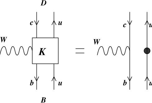
FIG. 1.: Pictorial demonstration of one particle approximation of the irreducible interaction kernel, filled circle denotes the inverse quark propagator

FIG. 2.: Form factors $R_{1}$ (long-dashed), $R_{2}$ (dashed-dotted), and $h_{A_{1}}$ for the $B\rightarrow D^{*}$ transition. The Isgur-Wise function $\xi$ of heavy quark mass limit is shown as solid line. Radiativ corrections not included here.

FIG. 3.: $|V_{cb}|{\cal F}(\omega)$ as a function of $\omega$ for $B\rightarrow D^{*}e\nu$ decays. Data points from CLEO and their linear fit (with $c=0$, dashed-dotted line). Model best fit is displayed as solid line. Long-dashed with the same value for $|V_{cb}|$ at $\omega=1$ but $R_{1,2}$ constant. Dashed line uses $V_{cb}$ from CLEO analysis and $R_{1,2}$ constant (i.e. zero-recoil method) for comparison.

FIG. 4.: $|V_{cb}|{\cal F}(\omega)$ as a function of $\omega$ for $B\rightarrow De\nu$ decays. Data points from CLEO and their linear fit (with $c=0$, dashed-dotted line). Model best fit is displayed as solid line, same $V_{cb}$ as in Fig. 3.

REFERENCES

- [1] R.M. Barnett et al., Phys. Rev. D 54, 1 (1996), and 1997 off-year partial update for the 1998 edition available on the PDG WWW pages (URL: http://pdg.lbl.gov/).
- [2] N. Isgur, M. B. Wise, Phys. Lett. B 232, (1989) 113; B 237, 527 (1990).
- [3] CLEO Collaboration, S. Sanghera et al., Phys. Rev. D 47, 791 (1993); B. Barish et al., Phys. Rev. D 51, 1014 (1995); J.E. Duboscq et al. Phys. Rev. Lett. 76 3898 (1996).
- [4] M. Wirbel, B. Stech, M. Bauer, Z. Phys. C 29, 637 (1985).
- [5] N. Isgur, D. Scora, B. Grinstein, M.B. Wise, Phys. Rev. D 39, 799 (1989).
- [6] W.Jaus, Phys. Rev. D 41 3394 (1990), ebd. D 53, 1349 (1996).
- [7] V.O. Galkin, A.Yu. Mishurov, R.N. Faustov, Sov. J. Nucl. Phys. 55 (1992) 1207, R.N. Faustov, V.O. Galkin, A.Yu. Mishurov, J. Nucl. Phys. 55 (1992) 1080 (english: JINR print Dubna, Russia E2-91-451), R.N. Faustov, V.O. Galkin, A.Yu. Mishurov, Phys. Lett. B 356, 516 (1995); ibid. B367 E391 (1996); R.N. Faustov, V.O. Galkin, Z. Phys. C 66, 119 (1995).
- [8] D. Scora, Nathan Isgur, Phys. Rev. D 52, 2783 (1995).
- [9] G. Zöller, S. Hainzl, C.R. Münz, M. Beyer, Z. Phys. C 68, 103 (1995); G. Zöller, diploma thesis (in German, unpublished, Bonn 1994).
- [10] I.L. Grach, I.M. Narodetskii, S. Simula, Phys. Lett. B 385, 317 (1996).
- [11] D. Melikov, Phys. Lett. B 394, 385 (1997), ibid. B 380 (1996), Phys. Rev. D 53, 2460 (1996).
- [12] H.-Y. Cheng, C.-Y. Cheung, C.-W. Hwang, Phys. Rev. D 55, 1559 (1997).
- [13] A. Le Yaouanc invited plenary talk on IVth International Workshop on Progess in Heavy Quark Physics held in Rostock 1997, to be published in the proceedings (eds. M. Beyer, T. Mannel, H. Schröder, Rostock University Press, 1998).
- [14] V. Braun invited plenary talk on IVth International Workshop on Progess in Heavy Quark Physics held in Rostock 1997, to be published in the proceedings (eds. M. Beyer, T. Mannel, H. Schröder, Rostock University Press, 1998).
- [15] C. Sachrajda invited plenary talk on IVth International Workshop on Progess in Heavy Quark Physics held in Rostock 1997, to be published in the proceedings (eds. M. Beyer, T. Mannel, H. Schröder, Rostock University Press, 1998).
- [16] B. Stech, Z. Phys. C 75, 245 (1997).
- [17] J. Resag, C.R. Münz, B.C. Metsch, H.R. Petry, Nucl. Phys. A 578 397 (1994).
- [18] C.R. Münz, J. Resag, B.C. Metsch, H.R. Petry, Nucl. Phys. A 578, 418 (1994).
- [19] C.R. Münz, J. Resag, B.C. Metsch, H.R. Petry, Phys. Rev. C52, 2110 (1995).
- [20] J. Resag, C.R. Münz, Nucl. Phys. A 590, 735 (1995).
- [21] J.F. Lagaë, Phys. Rev. D 45 305, 317 (1992).
- [22] H. Hersbach, Phys. Rev. A 46 3657 (1992), D 47 3027 (1993).
- [23] E. Hummel, J. Tjon, Phys. Rev. C 42, 423 (1990); G. Rupp, J.A. Tjon, Phys. Rev. C 41, 472 (1990); P.C. Tiemeijer, J.A. Tjon: Phys. Lett. B 277, 38 (1992); Phys. Rev. C49 494 (1993), C 48 896 (1994).
- [24] T. Murota, Progr. Theor. Phys. 69, 181 (1983), ibid. 1498 (1983).
- [25] Yu.L. Kalinovsky, C. Weiss: Z. Phys. C 63, 275 (1994).
- [26] E.E. Salpeter, H.A. Bethe, Phys. Rev. 84, 1232 (1951).
- [27] S. Mandelstam, Proc. Roy. Soc. 233, 248 (1955)
- [28] A. Bilal, P. Schuck, Phys. Rev. D 31, 2045 (1985).
- [29] E. Klempt, B.C. Metsch, C.R. Münz, H.R. Petry, Phys. Lett. B361, 160 (1995), W.I. Giersche, C.R. Münz, Phys. Rev. C 53, 2554 (1996), C.R. Münz, Nucl. Phys. A 609, 364 (1996).
- [30] J.G. Körner, G.A. Schuler, Z. Phys. C 38, 511 (1988) 511 [E C 41, 690 (1989)]; C 46, 93 (1990).
- [31] M. Neubert, Phys. Rep. 245, 259 (1994).
- [32] CLEO collaboration, G. Gollin invited plenary talk on IVth International Workshop on Progess in Heavy Quark Physics held in Rostock 1997, to be published in the proceedings (eds. M. Beyer, T. Mannel, H. Schröder, Rostock University Press, 1998).
- [33] S. Resag, M. Beyer, Z. Phys. C 63 121 (1994).
- [34] D. Lurie, Particles and Fields, (Interscience Publishers, 1968).
- [35] M. Neubert, Phys. Lett. B 264, 455 (1991).
- [36] A. Czarnecki, Phys. Rev. Lett. 76 4124 (1996).
- [37] M.E. Luke, Phys. Lett. B 252, 447 (1990).
- [38] A.F. Falk, M. Neubert, Phys. Rev. D47 2965, 2982 (1993).
- [39] T. Mannel, Phys. Rev., D 50 428 (1994).
- [40] M.A. Shifman, N.G. Uraltsev, A. Vainshtein, Phys. Rev. D51, 2217 (1995).
- [41] G. Martinelli, Nucl. Instrum. Meth. A 384, 241 (1996).