To appear in Phys. Lett. B, hep-ph/9712479

Spontaneous Generation of Pseudoscalar Mass in the U(3)$\times$U(3) Linear Sigma Model

Abstract

A novel, nonperturbative, way to generate chiral symmetry breaking within the linear sigma model for 3 flavours with an interaction term $\lambda{\rm Tr}[\Sigma\Sigma^{\dagger}\Sigma\Sigma^{\dagger}]$ is discussed. After spontaneous chiral symmetry breaking in the vacuum at the tree level the scalar nonet obtains mass, while the pseudoscalars are massless. Then, including quantum loops in a nonperturbative, self-consistent way chiral symmetry is broken by nonplanar graphs in a second step, and also the pseudoscalars become massive. By interpreting the basic symmetry to be a discrete permutation symmetry, in accord with superselection rules, no additional Goldstone bosons are expected.
Pacs numbers:12.39.Ki, 11.30.Hv, 11.30.Qc, 12.15.Ff

1. Introduction and the linear sigma model. Today the detailed experimental data on the light scalar and pseudoscalar mass spectrum and mixings defy any simple phenomenological explanation. It seems obvious that these mesons require a much better understanding of the nonperturbative and nonlinear aspects of QCD at low energies, than we have today. When hopefully in the near future these mesons are understood, we most probably have a much better understanding also of the confinement mechanism. This paper is an attempt to bridge this gap, and to understand hadron mass generation in general.

I shall first argue that a good candidate for an effective meson theory at low energies, when the gluonic degrees of freedom are integrated out, is the generalization of the well known linear sigma model[1, 2] to $U(3)\times U(3)$ including one scalar and one pseudoscalar nonet. I restrict myself generally to 3 light flavours ($N_{f}=3$), although sometimes I keep the $N_{f}$ in the formulas for clarity. Consider the basic $U(3)\times U(3)$ symmetric, classical Lagrangian, which has same flavour and chiral symmetries as QCD:

$${\cal L}=\frac{1}{2}{\rm Tr}[\partial_{\mu}\Sigma\partial_{\mu}\Sigma^{\dagger}]+\frac{1}{2}m^{2}{\rm Tr}[\Sigma\Sigma^{\dagger}]-\lambda{\rm Tr}[\Sigma\Sigma^{\dagger}\Sigma\Sigma^{\dagger}]-\lambda^{\prime}({\rm Tr}[\Sigma\Sigma^{\dagger}])^{2}+{\cal L}^{SB}\ .$$ (1)

Here $\Sigma=\sum_{a=0}^{8}(s_{a}+ip_{a})\lambda_{a}/\sqrt{2}$ are $3\times 3$ matrices, $s_{a}$ and $p_{a}$ stand for the $0^{++}$  and $0^{-+}$  nonets and $\lambda_{a}$ are the Gell-Mann matrices, normalized as ${\rm Tr}[\lambda_{a}\lambda_{b}]=2\delta_{ab}$, and where for the singlet $\lambda_{0}=(2/3)^{1/2}{\bf 1}$ is included. Note that each meson from the start has a definite $SU(3)$ symmetry content, which in the quark model means that it has a definite $q\bar{q}$ content. Thus the potential terms in Eq. (1) can be given a conventional quark line structure shown in Fig. 1.

FIG. 1.: Graphical quark line representation of the $\lambda$ and $\lambda^{\prime}$ terms of Eq. (1). Note the disconnected quark line nature of the $\lambda^{\prime}$ term.

Apart from the symmetry breaking term ${\cal L}^{SB}$, Eq. (1) is clearly invariant under $\Sigma\to U_{L}\Sigma U_{R}^{\dagger}$ of $U(3)\times U(3)$. In Eq. (1) I have contrary to the usual convention defined the sign of $m^{2}$ such that the naive physical squared mass would be $-m^{2}$, and the instability thus occurs when $m^{2}>0$.

If $-m^{2}<0$ and $\lambda>0,\lambda^{\prime}>0$ the potential in Eq. (1) (being of the form of a ”Mexican hat”) gives rise to an instability with vacuum condensate $<s_{0}>=(2/3)^{1/2}f_{\pi}$. Let $\lambda^{\prime}=0$. Then shifting as usual the scalar field, $\Sigma\rightarrow\Sigma+f_{\pi}{\bf 1}$, one finds $f_{\pi}^{2}=m^{2}/(4\lambda)$ (cf. Fig. 2). Furthermore, the squared mass ($-m^{2}$) of the $0^{++}$ nonet is replaced nonperturbatively by $-m^{2}+12\lambda f_{\pi}^{2}=2m^{2}$, while the $0^{-+}$ nonet becomes massless, $-m^{2}+4\lambda f_{\pi}^{2}=0$. The symmetry of the spectrum is broken down to $SU(3)\times U_{A}(1)$. If we had included the $\lambda^{\prime}$ term instead of the $\lambda$ term, then only the scalar singlet would aquire mass while the remaining 17 states would be massless. Then more symmetry remains in the spectrum; O(18) symmetry is broken down to O(17). More generally with both $\lambda$ and $\lambda^{\prime}$ present the scalar octet squared mass is $2m^{2}\lambda/(\lambda+3\lambda^{\prime})$, while the singlet squared mass is $2m^{2}$, and the 9 pseudoscalars are massless.

FIG. 2.: After shifting the field $\Sigma\to\Sigma+f_{\pi}$ (denoted by the blob) the $\lambda$ term in Fig. 1 generates the mass terms in a and b, $[4{\rm Tr}\Sigma\Sigma^{\dagger}+{\rm Tr}(\Sigma\Sigma+h.c.)]\lambda f_{\pi}^{2}$, and the trilinear couplings, $4\lambda f_{\pi}{\rm Tr}[\Sigma\Sigma\Sigma^{\dagger}+h.c.]/2$ shown in c, which are flavour symmetric and obey the OZI rule.

In addition, very importantly, after shifting the scalar singlet field, the $\lambda$ term (keeping $\lambda^{\prime}=0$) generates trilinear $spp$ and $sss$ couplings of the form $g{\rm Tr}[\Sigma\Sigma\Sigma^{\dagger}+h.c]/2$, (cf. Fig. 2c), where g is $g=4\lambda f_{\pi}$. With the flavour indices written out explicitly one has (not including the combinatoric factors)

$$g_{abc}=g{\rm Tr}[\lambda_{a}\lambda_{b}\lambda_{c}+\lambda_{a}\lambda_{c}\lambda_{b}]/(2\sqrt{8})\ .$$ (2)

These couplings obey the simply connected, Okubo-Zweig-Iizuka (OZI) allowed, quark line rules with flavour symmetry exact. One has SU(3)_f predictions relating different couplings constants. Denoting by $\sigma$ the $u\bar{u}+d\bar{d}$ scalar, and by $\sigma_{s}$ the $s\bar{s}$ scalar one has e.g. $g^{2}=2g^{2}_{\sigma\pi^{0}\pi^{0}}=g^{2}_{\sigma\pi^{+}\pi^{-}}=2g^{2}_{\sigma K\bar{K}}=\frac{4}{3}g^{2}_{K^{*}_{0}K\pi}=2g^{2}_{a_{0}K\bar{K}}=g^{2}_{\sigma_{s}K\bar{K}}$, and $g_{\sigma_{s}\pi\pi}=0$ etc. Here we summed over charge states except for the $\sigma\pi\pi$ couplings, since conventionally the $\sigma\pi\pi$ coupling is $g_{\sigma\pi^{0}\pi^{0}}$. If one includes also the $\lambda^{\prime}$ term of Eq. (1) then only the couplings involving the $\sigma$ and $\sigma_{s}$ states would be altered, which would violate the OZI rule at the tree level.

Conventionally one includes into $\cal{L}$ terms which break the symmetries:

$${\cal L}^{SB}=\epsilon_{0}s_{0}+\epsilon_{8}s_{8}+c\cdot[\det\Sigma+\det\Sigma^{\dagger}]\ .$$ (3)

Here $\epsilon_{0}$ gives, by hand, the pseudoscalar nonet a common mass, while $\epsilon_{8}$ breaks explicitly the remaining $SU(3)$   down to isospin. These terms are related to quark masses in QCD. Because of the quantum effects in QCD involving the gluon anomaly the $U_{A}(1)$ symmetry of Eq. (1) is broken. This is represented by the $c$ term in Eq. (3), which gives the $\eta_{1}$ an extra mass[4]. For most of the discussion below we shall neglect the $\epsilon_{8}$ and $c$ terms, except in the discussion of the fit to the scalar mesons below, where they enter through the $0^{-+}$  masses.

2. The U3$\times$U3 sigma model and scalar meson data. In this section I include some results of phenomenology for two reasons: (i) I want to emphasizes the fact that the U3$\times$U3 model discussed above is in fact phenomenologically a very successful model for the scalar mesons, and (ii) I need the parameters determined here in order to estimate the pseudoscalar mass in Eq. (11) below.

The flavour symmetric OZI rule obeying couplings of Eq. (2) together with a near-degenerate bare scalar nonet mass were, in fact, the starting point of our recent analysis of the scalar $q\bar{q}$ nonet [3]. In particular it was crucial that after determining the overall coupling $g$ from a fit to data on $K^{*}_{0}\to K\pi$ and $a_{0}\to\pi\eta$ one essentially predicted the $\pi\pi$ I=0 S-wave phase shift (Fig. 3). This shows that the above relations relating the bare $\sigma$ and $\sigma_{s}$ couplings to the same overall $g$ as those of $K^{*}_{0}K\pi$ and $a_{0}\pi\eta$ must be approximately satisfied experimentally. I.e., one cannot tolerate a very big bare $\lambda^{\prime}$ coupling in Eq. (1) since then these relations would be destroyed. Another argument for that $\lambda^{\prime}$ must be small is that then the bare scalar singlet state would have a very different mass from the other nonet members, not needed in the fit. After the unitarization the scalars aquired finite widths and were strongly shifted in mass by the different couplings to the $0^{-+}$$0^{-+}$ thresholds. The $0^{-+}$  masses in the thresholds were given their experimental values (i.e. we included effectively ${\cal L}^{SB}$ for the $0^{-+}$ states), and consequently the main source of flavour symmetry breaking in the output physical mass spectrum was generated by the vastly different positions of these thresholds. E.g. the large experimental splitting between the $a_{0}(980)$ and $K^{*}_{0}(1430)$ masses came from the large breaking in the sum of loops for the $K^{*}_{0}$ ($K^{*}_{0}\to K\pi,K\eta,K\eta^{\prime}\to K^{*}_{0}$) compared to those for $a_{0}$ ($a_{0}\to\pi\eta,K\bar{K},\pi\eta^{\prime}\to a_{0}$), although in the strict $SU(3)_{f}$ limit these thresholds would lie on top of each others and would then together give the same mass shift to the two resonances.

There were only 6 parameters in [3] out of which two parametrized the bare scalar spectrum (1.42 GeV for the $u\bar{u}$, $d\bar{d}$, $u\bar{d}$, $d\bar{u}$, and an extra 0.1 GeV when an $s$ quark replaces a $u$ or $d$ quark). The overall coupling was parametrized by $\gamma=1.14$, and $k_{0}=0.56$ GeV/c was the cut off parameter. Now, the $\gamma$ parameter can be related to $\lambda$ of Eq. (1) through $\lambda=4\pi\gamma^{2}=16$, by comparing the $\sigma\pi\pi$ coupling of the two schemes. [One has $g^{2}_{\sigma\pi^{0}\pi^{0}}/(4\pi)$ $=\gamma^{2}m^{2}_{\sigma}=\lambda m^{2}_{\sigma}/(4\pi)$. The latter equation follows from $g_{\sigma\pi^{0}\pi^{0}}=g/\sqrt{2}=4f_{\pi}\lambda$ and $f_{\pi}^{2}=m^{2}/(4\lambda)=m_{\sigma}^{2}/(8\lambda)$ given above.]

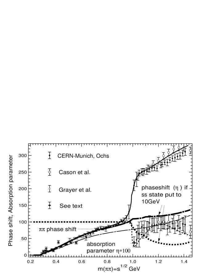
FIG. 3.: The full line curve shows the I=0, S-wave phase shifts for $\pi\pi\rightarrow\pi\pi$, as predicted by the model [3]. If one lets the $s\bar{s}$ meson mass become very large (10 GeV) then the rapid rise at 1 GeV due to the $f_{0}(980)$ vanishes. This shows that $f_{0}(980)$ is the unitarized $s\bar{s}$ state. The remaining phase shift (dot-dashed thick line) is then entirely due to the $u\bar{u}+d\bar{d}$ channel and one sees that what remains can be understood as a very broad resonance. This is the ”$\sigma$”, whose 90^∘ mass value is at 880 MeV, while the pole is at 470-i250 MeV. (The thin dot-dashed curve shows the phase shift if also the $K\bar{K}$ and $\eta\eta$ thresholds are given large values.)

Using the conventional value for $f_{\pi}=93$ MeV and $\lambda=16$ one predicts from (1) at the tree-level that $m_{\sigma}=f_{\pi}(8\lambda)^{1/2}$=1060 MeV as an average mass of the $u\bar{u},\ d\bar{d},\ d\bar{u}$ and $u\bar{d}$ states. Now although strictly speaking there is no exact one-one correspondence between the model of Eq. (1) at the tree level, before unitarization, and the unitarised model of [3], it is remarkable that this prediction is close to the average mass of the $a_{0}(980)$ and $\sigma$ resonances found in the fit. I.e. if we had used $f_{\pi}=93$ MeV to determine the energy scale, we could have eliminated one of the 6 parameters.

An important point observed in the second paper of Ref. [3] was that the model requires the existence of the light and broad $\sigma$ resonance pole. This is explained in more detail in Fig. 3. Recently there has appeared several new papers [5], which through different analyses and models support this same conclusion, i.e. that the light and broad sigma, which has been controversial for so long, really exists, and is here to stay [6].

The important conclusion of this phenomenological section is that the model of [3] can be interpreted as an effective field theory given by Eqs. (1) and (3) with $\lambda=16$ and $\lambda^{\prime}\approx 0$. (For other determinations of $\lambda$ and $\lambda^{\prime}$ where $\lambda^{\prime}$ generally is not small see [7]-[10]). The absence of the $\lambda^{\prime}$ term at the tree level means that the OZI rule holds exactly at the tree level. Of course the unitarization procedure can be improved upon, including u- and t-channel singularities [11], $s\to ss\to s$ loops, higher order diagrams etc., but I am confident that the dominant effects were already included phenomenologically for the scalar states.

3. Spontaneous generation of pseudoscalar mass. Let us now consider loops and renormalization. As is well known the linear sigma model is renormalizable, as first shown by Lee[2]. Crater[12] discussed the renormalization of the $U(3)\times U(3)$ symmetric model, Eq. (1), before spontaneous breaking and without ${\cal L}^{SB}$, and showed that the $\lambda$ term is not alone renormalizable but requires through loops the presence of the $\lambda^{\prime}$ coupling. This is not inconsistent with the result above that the bare $\lambda^{\prime}$ term must be small. Paterson[13] has showed that the Coleman-Weinberg[14] mechanism occurs when $\lambda\neq 0$ i.e, that the symmetry is spontaneously broken also in the case when the bare mass term $m$ is assumed to vanish. Thus the $\lambda$ term generally requires, after radiative corrections, the presence of both a nonvanishing mass term and a small $\lambda^{\prime}$ term in the renormalized Lagrangian. Furthermore, Chan and Haymaker[10] have discussed the renormalizability of the full Lagrangian (1), with the symmetry breaking term (3), and $<s_{0}>\neq 0$ present from the start.

Consider the lowest order loops generated by the Lagrangian (1) after shifting the scalar field, Figs. 4a,b and 5a,b. In these one loop integrals one needs the two familiar functions $A(m^{2})$ and $B(m_{1}^{2},m^{2}_{2})$, given below with a three momentum cut off. The simple function $A(m^{2})$ is the same one-loop function which appears in most gap equations, c.f.[15, 16].

$$A(m^{2}) = \int\frac{id^{4}k}{(2\pi)^{4}}[k^{2}-m^{2}+i\epsilon]^{-1}=\frac{1}{32\pi^{2}}\int^{4(\Lambda^{2}+m^{2})}_{4m^{2}}(1-4m^{2}/s)^{\frac{1}{2}}ds$$ (4)

$$= \frac{\Lambda^{2}}{8\pi^{2}}\Bigl{[}(1+\frac{m^{2}}{\Lambda^{2}})^{\frac{1}{2}}-\frac{m^{2}}{\Lambda^{2}}\ln[\frac{\Lambda}{m}(1+(1+\frac{m^{2}}{\Lambda^{2}})^{\frac{1}{2}})]\Bigr{]}\ .$$ (5)

$$B(m_{1}^{2},m^{2}_{2}) = \int\frac{id^{4}k}{(2\pi)^{4}}[(k^{2}-m_{1}^{2}+i\epsilon)(k^{2}-m_{2}^{2}+i\epsilon)]^{-1}=(m_{1}^{2}-m_{2}^{2})^{-1}[A(m_{1}^{2})-A(m_{2}^{2})]\ .$$ (6)

Denote the degenerate $0^{-+}$ octet masses (i.e. $\pi,K,\eta_{8}$) by $m_{p_{8}}$ and the degenerate $0^{++}$ octet masses ($a_{0},K^{*}_{0},\sigma_{8}$) by $m_{s_{8}}$, while the singlet mases are $m_{p_{0}}$ and $m_{s_{0}}$. When one can neglect the octet singlet splitting the two nonet masses are denoted $m_{s_{9}}$ and $m_{p_{9}}$.

FIG. 4.: The planar tadpole diagram (a) generated from the $\lambda$ term, the planar tadpole diagram (b) with an intermediate scalar singlet and the planar loop diagram (c) generated from the trilinear couplings in Fig. 2c. When flavour symmetry is unbroken these diagrams contribute equally to each member of a nonet, and the internal closed loop simply gives a factor $N_{f}$. Thus they have the same structure as the mass terms in the tree level Lagrangean and can be included in it as renormalization terms.

FIG. 5.: The nonplanar, OZI-rule violating one loop graphs, which contribute only to the singlet channels. These are nonvanishing when $<s_{0}>\neq 0$ and the scalars are massive and nondegenerate with the pseudoscalars. For the $0^{-+}$ singlet the sum of the one-loop digrams cancel (Eq. 7), but for the scalar singlet they add (Eq. 8) renormalizing the scalar singlet quadratic term differently from the rest.

There are two main classes of diagrams: the ”planar” diagrams of Fig. 4 and the disconnected OZI rule violating ”nonplanar” diagrams of Fig. 5. As long as $SU(3)_{f}$ remains unbroken one can sum over flavour in the planar graphs giving simply a factor $N_{f}$. Therefore these planar diagrams at most only renormalize the masses of the two nonets. For the pseudoscalar nonet one gets, (at $s=p^{2}=0$)

$$\Delta m^{2}_{p9}(planar) = N_{f}[(8\lambda-\frac{6g^{2}}{m^{2}_{s0}})A(m^{2}_{s_{9}})+(8\lambda-\frac{2g^{2}}{m^{2}_{s0}})A(m^{2}_{p_{9}})+2g^{2}B(m^{2}_{s_{9}},m^{2}_{p_{9}})]=$$ (7)

$$= \lambda N_{f}[(8-12+4)A(m^{2}_{s9})+(8-4-4)A(m^{2}_{p9})]\to 0\ ,$$ (8)

The loops generated directly from the $\lambda$ term Fig. 4a and 5a have a combinatoric factor of 12 out of which 8 are planar and 4 nonplanar. Therefore the two numbers 8 in Eq. (8). On the other hand the tadpole loops of Fig. 4b contribute the terms with the numbers $-12$ and $-4$ (when one uses the relation $2g^{2}/m^{2}_{s0}=4\lambda$). Finally the planar loops Fig. 4c, which give the $2g^{2}B$ term, contribute with the numbers $-4$ and $+4$, when one furthermore uses the relation (6). Similar cancellations whithin the standard sigma model including $\pi$ and $\sigma$ only have been studied by Bramon et al. [5], who also showed that if one adds quarks to the theory, and considers diagrams like Fig. 4b and 4c, but whithout the inner closed loop, also these diagrams cancel each other.

For the $0^{++}$ nonet one gets in a similar way a common mass shift to the whole nonet, which can be included into the bare nonet mass. One can consider the loop diagrams of Fig. 4c as the driving terms of the instability, which contribute to the negative curvature of the effective potential near the origin, and to the “wrong” sign $m^{2}$ term in Eq. (1). The tadpole terms then corresponds to how the vacuum responds, i.e. to the terms obtained through the vacuum condensate. Thus if we would restrict ourselves to including planar diagrams only, we would have a similar situation as at the tree level, with massless pseudoscalars and a massive scalar nonet.

However, there are of course also nonplanar diagrams, Fig. 5, which contribute only to the flavour singlet channels. Here the situation is more interesting (although in the large $N_{c}$ limit of QCD these would vanish). These diagrams give an extra contribution to the scalar singlet channel or the vacuum channel, which determines the vacuum condensate. There is an important minus sign whenever the nonet in the loop of Fig. 5a has the opposite parity than the external meson. This sign change can be seen from the negative sign of the last term in the expansion (see e.g.[17]) ${\rm Tr}[\Sigma\Sigma^{\dagger}\Sigma\Sigma^{\dagger}]={\rm Tr}[S^{4}]+{\rm Tr}[P^{4}]+4{\rm Tr}[S^{2}P^{2}]-2{\rm Tr}[PSPS]$, where $\Sigma=S+iP$, i.e., $S=\sum_{a}s_{a}\lambda_{a}/\sqrt{2}$ and $P=\sum_{a}p_{a}\lambda_{a}/\sqrt{2}$.

One can sum over scalar and pseudoscalar nonets in the loops of Fig. 5, and find for the $0^{-+}$ singlet:

$$\Delta m^{2}_{p_{0}}(nonplanar)=N_{f}\bigl{[}-4\lambda A(m^{2}_{s_{9}})+4\lambda A(m^{2}_{p_{9}})+2g^{2}B(m^{2}_{p_{9}},m^{2}_{s_{9}})\bigr{]}\to 0\ .$$ (9)

This sum vanishes exactly, when (i) the pseudoscalar masses vanish and (ii) when one neglects the small second order splitting between $s_{8}$ and $s_{1}$, because of the relation $g^{2}=2\lambda m^{2}_{s_{9}}$ (which, by the way, is the same relation which gives the Adler zeroes in $0^{-+}$$0^{-+}$ scattering). Then the contribution from Fig. 5a cancels that from Fig. 5b as seen from the relation between $A$ and $B$ in Eq. (6).

But, for the scalar singlet channel the signs of the two tadpole terms are opposite to that in Eq. (9) (again because of the important minus sign mentioned above) and one finds a nonvanishing result:

$$-\Delta\bar{m}^{2}_{0} = \Delta m^{2}_{s_{0}}(nonplanar)$$ (10)

$$= N_{f}\bigl{[}4\lambda A(m^{2}_{s_{9}})-4\lambda A(m^{2}_{p_{9}})+g^{2}B(m^{2}_{p_{9}},m^{2}_{p_{9}})+9g^{2}B(m^{2}_{s_{9}},m^{2}_{s_{9}})\bigr{]}\neq 0\ .$$ (11)

If one would evaluate this quantity using in the original Lagrangian, before shifting the scalar singlet field, i.e. when still $m_{s_{9}}=m_{p_{9}}$ and $g=0$, one would get zero also for this quantity. But, once the scalars and pseudoscalars are split in mass by the chiral symmetry breaking in the vacuum the loops in Fig. 5 are not anymore vanishing, and contribute to making $\Delta\bar{m}^{2}_{0}\neq 0$. Now I argue this does not only shift the scalars singlet mass slightly down from the scalar octet, but more importantly, because of self-consistency it also increases the instability in the scalar channel and thus also contributes to the shape of the potential, in a “second step of chiral symmetry breaking”:

The renormalized curvature of the potential in the scalar singlet direction will be bigger than in the other directions, i.e., ”the Mexican hat will be warped” by the extra quadratic term $-\frac{1}{2}\Delta\bar{m}^{2}_{0}s_{0}^{2}$.

The nonvanishing of $-\Delta\bar{m}^{2}_{0}$ in Eq. (8) is crucial in the following. It has the right negative sign making the quadratic term for the scalar singlet more negative than the corresponding term for the pseudoscalar nonet, and also more negative than the quadratic term for the scalar octet. This guarantees that the minimum of the renormalized potential will be in the direction of the scalar singlet, and that only chiral symmetry, not flavour nor parity, is violated in the solution.

Including this term into the stability condition that the linear term involving the scalar singlet should vanish one finds for the renormalized $f_{\pi}$.

$$f_{\pi}^{2}=(\bar{m}^{2}+\Delta\bar{m}_{0}^{2})/(4\lambda)\ ,$$ (12)

where all quantities $m^{2},\ \Delta\bar{m}^{2}_{0}$ and $\lambda$ are defined such that they normally are positive, when spontaneos symmetry breaking occurs.

Summing the different contribution to the four masses one finds

$$\begin{array}[]{rlllll}m^{2}_{s_{0}}&=-m^{2}-\Delta\bar{m}^{2}_{0}+12\lambda f_{\pi}^{2}&=2\Delta\bar{m}^{2}_{0}+2m^{2}&=8\lambda f_{\pi}^{2}\ ,\\ m^{2}_{s_{8}}&=-m^{2}+12\lambda f_{\pi}^{2}&=3\Delta\bar{m}^{2}_{0}+2m^{2}&=8\lambda f_{\pi}^{2}+\Delta\bar{m}^{2}_{0}\ ,\\ m^{2}_{p_{0}}\approx m^{2}_{p_{8}}&=-m^{2}+4\lambda f_{\pi}^{2}&=\ \Delta\bar{m}^{2}_{0}\ .\end{array}$$ (13)

Once the $0^{++}$ states are split from the $0^{-+}$ states through the first step of chiral symmetry breaking, then as a second step the nonplanar loops renormalize the potential with an extra quadratic term in the scalar singlet direction, $-\frac{1}{2}\Delta m^{2}_{0}s_{0}^{2}$.

FIG. 6.: The one loop diagram (a) generated from the $\lambda$ term, gives a contribution of the same disconnected flavour structure as the $\lambda^{\prime}$ term of Fig. 1b. Thus renormalization requires the presence of the $\lambda^{\prime}$ term in Eq. (1). Fig. 6b shows the tadpole graph which contributes to the scalar singlet channel. The blob on the internal line indicates that the vacuum insertions of Fig. 2a,b and loops of Fig. 5 should iteratively be included into the internal lines. This diagram is then nonvanishing if $<s_{0}>\neq 0$, when the scalars are massive and consequently the $0^{-+}$ and the $0^{++}$ states in the loop do not cancel. It has near the minimum the same flavour structure as the $\epsilon_{0}s_{0}$ term in Eq. (3). Thus renormalization requires its presence in and it gives the pseudoscalars mass.

It is of course very well known that renormalization deforms the effective potential from that of the tree level. Also, the fact that renormalization often requires the presence of new terms is well known. An example of the latter is provided by the fact that the $\lambda$ term of Eq. (1) requires the presence of a (small) $\lambda^{\prime}$ term [12], which we most easily can see graphically from Fig. 6a. The one loop correction generated from the $\lambda$ term shown in Fig. 6a has the same disconnected flavour structure as the $\lambda^{\prime}$ term of Eq. (1) and Fig. 1b. The unconventional new result presented here is that quantum effects, through the self-consistency condition, can also, nonperturbatively, generate new terms which violate the original symmetries of the tree Lagrangian.

Even this result is not quite new, the breaking of the $U_{A}(1)$ symmetry by the anomaly is another example of symmetry breaking through quantum effects. And in fact, the new mechanism also breaks the $U_{A}(1)$ symmetry albeit in a new and simpler way. The main difference is that not only the $\eta_{1}$, but the whole $0^{-+}$  nonet aquires mass, and that the effective potential obtains a quadratic symmetry breaking term, which warps the potential. Near the minimum the quadratic warping can be replaced by a conventional linear $\epsilon_{0}s_{0}$ term, as in Eq. (3), represented graphically by the nonvanishing diagram in Fig. 6b. Because of this the $0^{-+}$  nonet obtains a mass $\Delta\bar{m}_{0}$. Near the minimum this has the same effect as the conventional explicit symmetry breaking term $\epsilon_{0}s_{0}$ with $\epsilon_{0}\approx\Delta\bar{m}_{0}^{2}(2/3)^{1/2}f_{\pi}$.

4. Predicted pseudoscalar mass. What is the magnitude of the predicted pseudoscalar mass? It is clear that it really should depend only on the dimensionless coupling $\lambda$ evaluated at the appropriate scale, and the scalar mass (or $f_{\pi}$). In a forthcoming publication I shall make a more detailed instability calculation. Here, as a rough approximation choose the same parameters as in the fit to the scalar nonet: $\lambda(\approx 1$ GeV) =16, $\Lambda=560$ MeV/c, for the average nonet mass $m_{s_{9}}\approx 1$ GeV and for the input average pseudoscalar mass a range between 0 and 500 MeV. One finds from Eqs. (8) and Eq. (10) (neglecting the $g^{2}B$ terms which would increase the predicted $0^{-+}$ mass somewhat) for $N_{f}=3$

$$m_{p_{8}}\approx\bigl{[}4N_{f}\lambda[A(m^{2}_{p_{8}})-A(m^{2}_{s_{8}})]\bigr{]}^{1/2}=450\pm 200{\rm MeV}.$$ (14)

Using for the average $0^{-+}$ input mass 450 MeV one gets also 450 MeV for the output. This can be compared with the average experimental pseudoscalar octet mass of 368 MeV. This estimate is probably fortuitous, but already the fact that one gets the right order of magnitude is highly nontrivial, and shows that my mechanism can predict reasonable $0^{-+}$ masses. Certainly, the comparison with experiment can be improved upon by a more detailed calculation, and by including $SU(3)_{f}$ breaking, vector mesons, the running of the coupling $\lambda(\mu)$ etc. Qualitatively one expects that the running of coupling constant, in analogy with $\phi^{4}$ theory, decreases $\lambda$ as one moves from the 1 GeV region where it was determined down to the pseudoscalar masses. This would also reduce the predicted $0^{-+}$ masses. But the calculation of the $\beta$ function for the present model is a complicated matter indeed, especially as one would have to keep the detailed analytical threshold behaviour for the large number of thresholds involved.

5. The self-consistency condition. The essential condition, which I have imposed is that the same physical masses should be used for the ”input” masses in the loops on the r.h.s. of the equations as obtained for the ”output” physical masses on the l.h.s of Eqs. (13). This is as any self-consistency condition ”circular” in the sense that one way of solving it is by iteration, inserting the output masses into the input masses. This generates diagrams with loops and vacuum insertions within loops ad infinitum.

With this condition the potential is deformed by quantum corrections in such a way that the axial vector symmetry in the original tree-level Lagrangian is broken. One obtains when including quantum effects

$${\cal L^{\prime}}={\cal L}+\frac{1}{2}\Delta m_{0}^{2}s_{0}^{2}\ ,$$ (15)

where ${\cal L}$ now does not include ${\cal L}^{SB}$. Instead, the new term is generated through the loops of Fig. 5. It looks just like a term which explicitly breaks the symmetry, but is in fact, generated through the self-consistency condition for the potential. (Formally one could eliminate the new term by adding, by hand, a renormalization counter term adjusted in such a way that the new term is exactly cancelled. But then one would have to again add a similar term, by hand, in order to give the pseudoscalars mass. Such a procedure would of course be ridiculous; it is more natural to consider the tree level Lagrangian (1) to be fundamental, but its symmetries broken by quantum effects.)

Clearly Ward identities involving the divergence of the axial vector current will look different when derived from ${\cal L}$ than from ${\cal L}^{\prime}$. With the new term in ${\cal L}^{\prime}$  the Ward identities for the divergence of the axial vector currents will look just like the conventional ones where a pseudoscalar mass (or quark mass in QCD) is put in by hand. The main difference is that now the symmetry violating term is not put in by hand, but is evaluated through the self-consistency condition from the three level Lagrangian (1). Assuming the usual relations between quark masses and pseudoscalar masses in QCD, this would imply spontaneous generation of quark masses. This mechanism also opens up the door to a better understanding of the next step of symmerty breaking: the spontaneous breaking of $SU(3)$ flavour symmetry discussed in previous papers [18].

6. Spontaneous or explicit symmetry breaking. Goldstone bosons. Above I have called the second step in the symmetry breaking spontaneous, since it follows naturally from the first step once quantum effects are included into the classical Lagrangian (1). However, in the terminology of t’Hooft[4] symmetry breaking should be called spontaneous only if there appears Goldstone bosons, otherwise the symmetry breaking is explicit. Therefore t’Hooft calls the mass generation of the $\eta^{\prime}$ through the quantum effects related to the gluon anomaly an explicit symmetry breaking. If one adopts this convention also our symmetry breaking should be called explicit, i.e. not spontaneous, since also in our case the symmetry breaking is quantum mechanical and no related Goldstone bosons seem to exist.

We know experimentally that no additional scalar massless bosons related to our second step of chiral symmetry breaking have been observed (at least not as free particles, i.e. not counting confined ghosts, schizons or gluons). How then, can the Goldstone theorem be circumvented? We note that the simplest way out is to observe, that in Eq. (1) one really does not need the full continuous U3$\times$U3 symmetry. One can replace it with a discrete permutation symmetry where parity and flavour indices are permuted and still get the same constraints with degenerate mass for the whole scalar and pseudoscalar nonets before any symmetry breaking takes place. It is true that it is practical to embed this permutation symmetry into a larger continuous unitary group, but it is really not necessary.

Furthermore, one should remember that we do have superselection rules[19] of parity, charge, and generally flavour in strong interactions. E.g. superpositions of different charge states, say $\pi^{+}$ and $\pi^{0}$, or superpositions of $\pi^{+}$ and $a_{0}^{+}$, are not physically realizable states, in the same way as, say, different spin states are. I.e., the physical Hilbert space only includes the discrete states of definite flavour and parity, not superpositions of these, which are generated by the full continuous group. With this limitation in mind it is, in fact, more natural to look at flavour and chiral symmetry of strong interactions as a discrete symmetry. Then there is no conflict with the Goldstone theorem, since a discrete symmetry can broken spontaneously (or explicitly) without the appearance of Goldstones.

7. Concluding remarks. Finally my approach has two extra benefits which I find worth mentioning: (i) it puts the ”mysterious” OZI rule and its breaking through loops on a firmer Lagrangian framework through the dominance of the $\lambda$ term at the tree level in Eq. (1), and (ii) it may provide a resolution to the strong CP problem, since a quark mass can be put zero in the original tree level Lagranian, although an effective mass is generated through the spontaneous chiral symmetry breakdown in loops.

Acknowledgements. I thank C. Montonen, D.O. Riska, M. Roos and M. Sainio for useful comments, and H. Leutwyler, E. de Rafael and S. Weinberg for e-mail correspondence emphasizing the problem of Goldstone bosons, which led to the inclusion of section 6.

REFERENCES

- [1] J. Schwinger, Ann. Phys. 2 (1957) 407, M. Gell–Man and M. Levy, Nuovo Cim. XVI (1960) 705.
- [2] B. W. Lee, Nucl. Phys. B9 (1969) 649.
- [3] N. A. Törnqvist, Z. Physik C68 647 (1995); N. A. Törnqvist and M. Roos, Phys. Rev. Lett. 76 (1996) 1575.
- [4] G. t’Hooft, Phys. Rep. 142 (1986) 357, see especially section 6.
-
[5]
J. A. Oller and E. Oset, (hep-ph/971554)
and Nucl. Phys. A620 (1997) 438;
S. Ischida et al. Prog. Theor. Phys. 95 (1995) 745;
R. Kaminski et al. Phys. Rev. D50 (1994) 3145;
L.R. Baboukhadia et al., J. Phys. G23 (1997) 1065;
A. Bramon et al. J. Phys. G 24 (1998) 1;
M. Harada et al. Phys. Rev. Lett. (Comment) 78 (1997) 1603; N.A, Törnqvist and M. Roos, ibid 78 (1997) 1604;
M.D. Scadron, ”Scalar meson via chiral and crossing dynamics” hep-ph/9710317;
See also M. Boglione and M. Pennington, Phys. Rev. Lett. 79 (1997) 1998. - [6] R. M. Barnett et al., (The Particle Data Group), Phys. Rev. D54 (1996) 1.
- [7] R. D. Pisarski and F. Wilczek, Phys. Rev. D29 (1984) 338.
- [8] S. Gavin, et al., Phys. Rev. D49 (1994) R3079.
-
[9]
H. Meyer-Ortmanns et al. Phys. Lett. B 295 (1992) 255;
H. Meyer-Ortmanns and B.-J. Schaefer, Phys.Rev D53 (1996) 6586. - [10] L.-H. Chan and R. W. Haymaker, Phys. Rev. D7 (1973) 402 and 415.
- [11] N. Isgur and J. Speth, Phys. Rev. Lett. (Comment) 77 (1996) 2332; N.A, Törnqvist and M. Roos, ibid 77 (1996) 2333.
- [12] H.C. Crater, Phys. ReV. D 1 (1970) 3313.
- [13] A.J. Paterson, Nucl. Phys. B190 (181) 188.
- [14] S. Coleman and E. Weinberg, Phys. Rev, D7 (1973) 1888.
- [15] Y. Nambu, G. Jona-Lasinio, Phys. Rev. 122 (1961) 345.
- [16] T. Hatsuda and T. Kunihiro, Phys. Rep. 247 (994) 223; S.P Klevansky, Rev. Mod. Physics 64 (1992) 643.
- [17] S. Gasiorowicz and D.A. Geffen, Rev. Mod. Phys. 41 (1969) 531.
- [18] N.A. Törnqvist, Physics Letters B406 (1997) 70; hep-ph/9612238; hep-ph/9703262.
-
[19]
G.C. Wick, A.S. Wightman and E.P. Wigner, Phys.Rev. 88
(1952) 101;
A.S. Wightman, Nuovo Cimento 110 (1995) 751.