Two Pion Correlations as a Possible Experimental Probe for Disoriented Chiral Condensates

Abstract

We discuss two-pion correlations as a possible experimental probe into disoriented chiral condensates. In particular, we point out that the iso-singlet squeezed states of the BCS type have peculiar two-particle correlations in the back-to-back and the identical momentum configurations which should be detectable experimentally. We motivate the examination of the squeezed state by showing that such state naturally appears in a final stage of nonequilibrium phase transitions via the parametric resonance mechanism proposed by Mrówczyński and Müller.

The disoriented chiral condensate (DCC)[1] is an intriguing idea for explaining possible large fluctuations of neutral to charge ratio which might be seen in the cosmic ray experiments [2]. A possible picture of DCC is as follows; The hot debris formed in high-energy hadronic collisions rapidly cools down so that chirally misaligned metastable “vacuum” like states are formed. They then relax to the QCD vacuum configuration by coherently emitting pions, and/or by dynamically producing pions via the parametrically amplified resonance mechanism.

Experimental search for the formation of DCC has been carried out by the MiniMax experiment at Fermilab [3]. Thanks to the well controlled experimental conditions of the accelerator experiments, they have a good chance of seeing the signature of DCC by observing large neutral to charge fluctuations. At least up to this moment, however, a clear signature for DCC does not appear to be found.

The experimental hunting of the signature of DCC so far relies on the analysis of global quantities such as multiplicity distributions and the correlations between charged and neutral particles. Let us consider the following possibility: Suppose that DCC forms in hadronic collisions but with a tiny probability, for example 1% or even 0.1%. Then, one may ask the question “is it possible for such global analysis at hand to signal the DCC formation?”. The answer is likely to be no. This is the real worry because no one ever made attempt to compute, or even estimate, the formation probability of DCC in hadronic collisions.

We propose in this paper that two-pion correlations may serve as a good indicator for DCC. The two-particle correlation functions are experimentally measurable quantities and have been used as a sensitive probe for clustering in multiparticle final states [4], and for measuring size of the clusters by the quantum mechanical interference between identical particles, the Hanbury-Brown-Twiss effect [5].

Two-particle correlations can work as an appropriate measure for DCC formation provided that the two-particle correlations in the DCC events have different characteristic features from those of non-DCC events. We argue that it indeed is the case for broad class of models in which the produced multi-pion states can be described by the squeezed states.

It has been suggested by Amado and Kogan [7] that the quantum pion states produced in DCC can be described by the squeezed state. The global quantities such as multiplicity distributions and correlations are calculated without specifying pion charges in Refs. [7, 8].

We explore in this paper a different mechanism which leads to the iso-singlet squeezed state with momentum correlation of the BCS type. It leads to definite predictions of the two-pion correlations with various charge and momentum combinations. Although not entirely model-independent, measuring the two-pion correlation functions may provide an alternative strategy for hunting the formation of DCC.

Toward the goal we organize this paper in the following two steps:
(A) We discuss a concrete model proposed by Mrówczyński and Müller [9] based on the parametric resonance mechanism to draw a physical picture behind the multi-pion squeezed state.
(B) We then extract the characteristic features of two-pion correlations implied by the squeezed pion state itself which is independent of the dynamical model behind the states. A reader who is keenly interested in relatively model-independent consequences of the iso-singlet pion squeezed state can skip the part (A).

Let us start by introducing the model of multipion production from DCC to make our discussions concrete. We treat the linear $\sigma$ model within the approximation discussed by Mrówczyński and Müller [9]. We define the dynamical variables $\chi$ and $\vec{\pi}$ by expanding the $\sigma$ model fields around the minimum of the tilted wine-bottle potential as $\sigma=v+\chi$ and $\vec{\pi}=\vec{\pi}$. We further expand the dynamical variables around the harmonic background of $\chi$ as

$$\chi(\mbox{\boldmath$x$},t) = \chi_{0}\cos(m_{\sigma}t+\phi)+\hat{\chi}(\mbox{\boldmath$x$},t),$$ (1)

$$\vec{\pi}(\mbox{\boldmath$x$},t) = \hat{\vec{\pi}}(\mbox{\boldmath$x$},t).$$ (2)

By doing this, we take an intuitive semiclassical picture for nonequilibrium phase transition in which the sigma-model fields roll down along the $\sigma$ direction and oscillate around a minimum of the wine-bottle potential.

We use a Fourier transformed variable $Q_{\mbox{\boldmath$k$}}$ defined by

$\displaystyle\hat{\chi}(\mbox{\boldmath$x$},t)=\displaystyle\int\frac{d^{3}k}{(2\pi)^{3}}e^{i\mbox{\boldmath$k$}\cdot\mbox{\boldmath$x$}}Q_{\mbox{\boldmath$k$}}(t).$

For compactness, we always omit the similar expressions for pions whenever they arise in an analogous way of $\sigma$’s. In spite of the continuum notation above and hereafter we will be actually dealing with the theory quantized in a large but finite box. We hope that no confusion occurs with our notation. The Hamiltonian can be expressed in terms of $Q_{\mbox{\boldmath$k$}}$ and its canonical conjugate $P_{\mbox{\boldmath$k$}}=\dot{Q}_{-\mbox{\boldmath$k$}}$ as

$\displaystyle H=\displaystyle\int d^{3}k\left[\frac{1}{2}P_{\mbox{\boldmath$k$}}P_{-\mbox{\boldmath$k$}}+\frac{1}{2}\Omega_{\mbox{\boldmath$k$}}^{\sigma}(t)^{2}Q_{\mbox{\boldmath$k$}}Q_{-\mbox{\boldmath$k$}}\right]+\sum_{a}\int d^{3}k\left[\frac{1}{2}P_{\mbox{\boldmath$k$}}^{a}P_{-\mbox{\boldmath$k$}}^{a}+\frac{1}{2}\Omega_{\mbox{\boldmath$k$}}^{\pi}(t)^{2}Q_{\mbox{\boldmath$k$}}^{a}Q_{-\mbox{\boldmath$k$}}^{a}\right],$

where

$$\Omega_{\mbox{\boldmath$k$}}^{\sigma}(t)^{2} = \mbox{\boldmath$k$}^{2}+m_{\sigma}^{2}+3m_{\sigma}^{2}\left(\frac{\chi_{0}}{v}\right)\cos(m_{\sigma}t+\phi),$$ (3)

$$\Omega_{\mbox{\boldmath$k$}}^{\pi}(t)^{2} = \mbox{\boldmath$k$}^{2}+m_{\pi}^{2}+m_{\sigma}^{2}\left(\frac{\chi_{0}}{v}\right)\cos(m_{\sigma}t+\phi).$$ (4)

The index $a$ runs over 1-3 and we take the adjoint representation for the pion fields.

We restrict ourselves in this paper to the region of small oscillations, $\displaystyle\frac{\chi_{0}}{v}<\left(\frac{m_{\pi}}{m_{\sigma}}\right)^{2}$, so that the time-dependent frequency $\Omega_{\mbox{\boldmath$k$}}^{\pi}(t)$ for pions is always real. Unless this restriction is made $\Omega_{\mbox{\boldmath$k$}}^{\pi}(t)$ becomes imaginary for certain period of time at low momenta and it gives rise to another instability in the system. We will discuss this problem in our forthcoming publication. Under the above restriction the frequency for $\sigma$ automatically stays real.

We follow Shtanov, Traschen and Brandenberger [10] to obtain the quantum description of the multi-pion (and $\sigma$) states produced through the parametric resonance mechanism. The Hamiltonian can be diagonalized by using the time-dependent creation and the annihilation operators

$$a_{\mbox{\boldmath$k$}}(t) = \displaystyle\frac{1}{\sqrt{2\Omega_{\mbox{\boldmath$k$}}}}e^{i\int^{t}dt^{\prime}\Omega_{\mbox{\boldmath$k$}}(t^{\prime})}[\Omega_{\mbox{\boldmath$k$}}Q_{\mbox{\boldmath$k$}}+iP_{-\mbox{\boldmath$k$}}],$$ (5)

$$a_{\mbox{\boldmath$k$}}^{\dagger}(t) = \displaystyle\frac{1}{\sqrt{2\Omega_{\mbox{\boldmath$k$}}}}e^{-i\int^{t}dt^{\prime}\Omega_{\mbox{\boldmath$k$}}(t^{\prime})}[\Omega_{\mbox{\boldmath$k$}}Q_{-\mbox{\boldmath$k$}}-iP_{\mbox{\boldmath$k$}}],$$ (6)

and the analogous expressions for pions with superscript $a$ as

$\displaystyle H=\int d^{3}k(\Omega_{\mbox{\boldmath$k$}}^{\sigma}a_{\mbox{\boldmath$k$}}^{\dagger}a_{\mbox{\boldmath$k$}}+\sum_{a}\Omega_{\mbox{\boldmath$k$}}^{\pi}a_{\mbox{\boldmath$k$}}^{a\dagger}a_{\mbox{\boldmath$k$}}^{a}).$

We now discuss the sigma and the pion sector collectively because they are decoupled with each other. The Heisenberg equation of motion

$\displaystyle\dot{a}_{\mbox{\boldmath$k$}}(t)=\displaystyle\frac{\partial}{\partial t}a_{\mbox{\boldmath$k$}}(t)+i[H,a_{\mbox{\boldmath$k$}}]$

satisfied by the operators $a_{\mbox{\boldmath$k$}}(t)$ and $a_{\mbox{\boldmath$k$}}^{\dagger}(t)$ takes the form

$$\dot{a}_{\mbox{\boldmath$k$}}(t)=\displaystyle\frac{\dot{\Omega}_{\mbox{\boldmath$k$}}}{2\Omega_{\mbox{\boldmath$k$}}}e^{2i\int^{t}dt^{\prime}\Omega_{\mbox{\boldmath$k$}}(t^{\prime})}a_{-\mbox{\boldmath$k$}}^{\dagger}(t)$$ (7)

and its hermitian conjugate for $a_{\mbox{\boldmath$k$}}^{\dagger}$, where the dot implies the time derivative. The solution of these equation can be obtained by introducing the time-independent operators $b_{\mbox{\boldmath$k$}}$ and $b_{\mbox{\boldmath$k$}}^{\dagger}$ as

$$a_{\mbox{\boldmath$k$}}(t) = \alpha_{\mbox{\boldmath$k$}}(t)b_{\mbox{\boldmath$k$}}+\beta_{\mbox{\boldmath$k$}}^{*}(t)b_{-\mbox{\boldmath$k$}}^{\dagger},$$ (8)

$$a_{\mbox{\boldmath$k$}}^{\dagger}(t) = \beta_{\mbox{\boldmath$k$}}(t)b_{-\mbox{\boldmath$k$}}+\alpha_{\mbox{\boldmath$k$}}^{*}(t)b_{\mbox{\boldmath$k$}}^{\dagger}.$$ (9)

The commutation relation $[b_{\mbox{\boldmath$k$}},b_{\mbox{\boldmath$k^{\prime}$}}^{\dagger}]=\delta_{\mbox{\boldmath$k$},\mbox{\boldmath$k^{\prime}$}}$ implies that

$\displaystyle|\alpha_{\mbox{\boldmath$k$}}|^{2}-|\beta_{\mbox{\boldmath$k$}}|^{2}=1.$

It is nothing but the Bogoliubov transformation but one must notice that $b_{\mbox{\boldmath$k$}}$ and $b_{\mbox{\boldmath$k$}}^{\dagger}$ do not diagonalize the Hamiltonian. They are introduced to solve the Heisenberg equation (7) but not to diagonalize the Hamiltonian. The $a_{\mbox{\boldmath$k$}}$ and $a^{\dagger}_{\mbox{\boldmath$k$}}$ in (9) solve the equation (7) if $\alpha_{\mbox{\boldmath$k$}}$ and $\beta_{\mbox{\boldmath$k$}}$ obey the equations

$$\dot{\alpha}_{\mbox{\boldmath$k$}}(t^{\prime}) = \displaystyle\frac{\dot{\Omega}_{\mbox{\boldmath$k$}}}{2\Omega_{\mbox{\boldmath$k$}}}e^{2i\int^{t}dt^{\prime}\Omega_{\mbox{\boldmath$k$}}(t^{\prime})}\beta_{-\mbox{\boldmath$k$}},$$ (10)

$$\dot{\beta}_{\mbox{\boldmath$k$}}(t) = \displaystyle\frac{\dot{\Omega}_{\mbox{\boldmath$k$}}}{2\Omega_{\mbox{\boldmath$k$}}}e^{-2i\int^{t}dt^{\prime}\Omega_{\mbox{\boldmath$k$}}(t^{\prime})}\alpha_{-\mbox{\boldmath$k$}}$$ (11)

We define the vacua $|0\rangle$ and $|0(t)\rangle$ as

$$b_{\mbox{\boldmath$k$}}|0\rangle = 0,$$ (12)

$$a_{\mbox{\boldmath$k$}}(t)|0(t)\rangle = 0,$$ (13)

and require that $|0(t=0)\rangle=|0\rangle$. It leads to the initial conditions

$$\alpha_{\mbox{\boldmath$k$}}(0)=1,\;\beta_{\mbox{\boldmath$k$}}(0)=0.$$ (14)

A physical quantum of momentum $k$ is created (annihilated) by $a_{\mbox{\boldmath$k$}}^{\dagger}(t)$ ($a_{\mbox{\boldmath$k$}}(t)$) out of the vacuum $|0(t)\rangle$ because they are the variables that diagonalize the Hamiltonian at every time $t$. On the other hand, the quantum sigma state in DCC may be identified by $|0\rangle$.

Because of the Bogoliubov transformation (9) the $\sigma$ state $|0\rangle$ in DCC can be expressed by physical $\sigma$ quanta as

$$|0\rangle=\prod_{\mbox{\boldmath$k$}}\displaystyle\frac{1}{\sqrt{|\alpha_{\mbox{\boldmath$k$}}(t)|}}\mbox{exp}\left[\frac{\beta^{*}_{-\mbox{\boldmath$k$}}}{2\alpha^{*}_{\mbox{\boldmath$k$}}}a^{\dagger}_{\mbox{\boldmath$k$}}(t)a^{\dagger}_{-\mbox{\boldmath$k$}}(t)\right]|0(t)\rangle.$$ (15)

It may be appropriate to denote it as the squeezed state of the BCS type, as we do in this paper, because of the pairing between $k$ and $-\mbox{\boldmath$k$}$ modes. The states of the generic type of (15) are the squeezed states that is widely discussed in quantum optics [11]. We also note that the particle production via the parametric resonance has been extensively discussed in the context of reheating in the inflationary universe [10, 12, 13, 14].

We write the solution of the Heisenberg equation

$$\ddot{Q}_{\mbox{\boldmath$k$}}(t)+\Omega^{2}_{\mbox{\boldmath$k$}}(t)Q_{\mbox{\boldmath$k$}}(t)=0$$ (16)

as

$\displaystyle Q_{\mbox{\boldmath$k$}}(t)=Q^{(-)}_{\mbox{\boldmath$k$}}(t)b_{\mbox{\boldmath$k$}}+Q^{(+)}_{\mbox{\boldmath$k$}}(+)b_{-\mbox{\boldmath$k$}}^{\dagger}.$

Where $Q^{(-)}_{\mbox{\boldmath$k$}}$ and $Q^{(+)}_{\mbox{\boldmath$k$}}$ are the solutions of the classical Mathieu equation (16) [15]. They satisfy $Q^{*(-)}_{\mbox{\boldmath$k$}}=Q^{(+)}_{-\mbox{\boldmath$k$}}$. It is easy to show that $\alpha_{\mbox{\boldmath$k$}}$ and $\beta_{\mbox{\boldmath$k$}}$ can be expressed as

$$\alpha_{\mbox{\boldmath$k$}}(t) = \displaystyle\frac{1}{\sqrt{2\Omega_{\mbox{\boldmath$k$}}}}e^{i\int^{t}dt^{\prime}\Omega_{\mbox{\boldmath$k$}}}\left[\Omega_{\mbox{\boldmath$k$}}Q^{(-)}_{\mbox{\boldmath$k$}}+i\dot{Q}^{(-)}_{\mbox{\boldmath$k$}}\right],$$ (17)

$$\beta_{-\mbox{\boldmath$k$}}(t) = \displaystyle\frac{1}{\sqrt{2\Omega_{\mbox{\boldmath$k$}}}}e^{-i\int^{t}dt^{\prime}\Omega_{\mbox{\boldmath$k$}}}\left[\Omega_{\mbox{\boldmath$k$}}Q^{(-)}_{\mbox{\boldmath$k$}}-i\dot{Q}^{(-)}_{\mbox{\boldmath$k$}}\right].$$ (18)

By including the pion degrees of freedom the quantum state of DCC in the Mrówczyński-Müller model can be written as

$$|0\rangle^{\sigma}\otimes|0\rangle^{\vec{\pi}}\equiv|\psi\rangle.$$ (19)

One of the most important feature of the state (19) is that it is the iso-singlet state. It comes from the fact that the frequency $\Omega_{\mbox{\boldmath$k$}}^{\pi}$ is isospin singlet.

Once the state is specified it is easy to compute the expectation values of the number densities of pion and $\sigma$ quanta. We use the collective notation

$\displaystyle\langle n\rangle^{\alpha}_{\mbox{\boldmath$k$}}\equiv\langle\psi|{a_{\mbox{\boldmath$k$}}^{\alpha}}^{\dagger}(t)a_{\mbox{\boldmath$k$}}^{\alpha}(t)|\psi\rangle,$

where $\alpha$ runs $\sigma$ and $\pi^{a}(a=+,-,0)$. Here, we use the representation of pion fields with definite charge states. Then,

$\displaystyle\langle n\rangle^{\alpha}_{\mbox{\boldmath$k$}}=|\beta_{\mbox{\boldmath$k$}}^{\alpha}|^{2}.$

We will comment on the question of how we should interpret the production of $\sigma$ quanta at the end of this paper.

We give in Fig. 1 the single pion momentum distributions calculated by the parametric resonance mechanism. They are identical for $\pi^{+}$, $\pi^{-}$ and $\pi^{0}$ because $|\psi\rangle$ is isospin singlet. The $\sigma$ model parameters are taken as follows: $m_{\pi}=140$ MeV, $m_{\sigma}=600$ MeV and $\displaystyle\frac{\chi_{0}}{v}=\frac{1}{20}$. The function $\beta_{\mbox{\boldmath$k$}}$ is computed by solving the Mathieu equation subject to the boundary condition (14). We observe a sharp peak at around $k=270$ MeV which is attributable to the first instability band of the Mathieu equation. An another peak due to the second resonance band which should exist at around $k=580$ MeV is too sharp to be visible in a finite-size binning. If we take the larger value of $\displaystyle\frac{\chi_{0}}{v}$ the peak widths become wider. If these spikes are not masked by the non-DCC backgrounds then it provides a sensitive experimental signature for the parametric resonance mechanism.

Now we move on to the part (B) to address the observable consequences of the squeezed state of the BCS type (19). We are interested in two-pion correlations. To this goal we first compute the two-particle momentum distributions of pions. They are defined as

$\displaystyle\langle\pi^{a}_{\mbox{\boldmath$k$}},\pi^{b}_{\mbox{\boldmath$k^{\prime}$}}\rangle\equiv\langle\psi|a^{a\dagger}_{\mbox{\boldmath$k$}}(t)a^{a}_{\mbox{\boldmath$k^{\prime}$}}(t)a^{b\dagger}_{\mbox{\boldmath$k^{\prime}$}}(t)a^{b}_{\mbox{\boldmath$k^{\prime}$}}(t)|\psi\rangle.$

Because of the factorized form of the state $|0\rangle^{\vec{\pi}}$ as in (15) we expect that the nontrivial (= not manifestly factorizable) two-pion distributions arise only in the sector of the identical and the back-to-back momentum configurations. In the computation of these quantities we further recognize that the two-pion distributions at zero-momentum can not be obtained by taking the smooth limit $\mbox{\boldmath$k$}\rightarrow 0$ of the expressions of either identical or back-to-back momentum configurations. It is because $a_{\mbox{\boldmath$k$}=0}$ and $a^{\dagger}_{\mbox{\boldmath$k$}=0}$ do not commute, whereas $a_{\mbox{\boldmath$k$}}$ and $a^{\dagger}_{-\mbox{\boldmath$k$}}$ do commute for $\mbox{\boldmath$k$}\neq 0$. Therefore, we have to compute three types of the two-pion distributions separately. We only quote the result leaving the details (which are not difficult to work out) to our forthcoming paper [16].
(a) identical momentum distribution:

$$\langle\pi^{+}_{\mbox{\boldmath$k$}},\pi^{+}_{\mbox{\boldmath$k$}}\rangle = \langle\pi^{0}_{\mbox{\boldmath$k$}},\pi^{0}_{\mbox{\boldmath$k$}}\rangle=\langle n\rangle_{\mbox{\boldmath$k$}}\left(2\langle n\rangle_{\mbox{\boldmath$k$}}+1\right),$$ (20)

$$\langle\pi^{+}_{\mbox{\boldmath$k$}},\pi^{-}_{\mbox{\boldmath$k$}}\rangle = \langle n\rangle^{2}_{\mbox{\boldmath$k$}}.$$ (21)

(b) back-to-back momentum distribution:

$$\langle\pi^{+}_{\mbox{\boldmath$k$}},\pi^{-}_{-\mbox{\boldmath$k$}}\rangle = \langle\pi^{0}_{\mbox{\boldmath$k$}},\pi^{0}_{-\mbox{\boldmath$k$}}\rangle=\langle n\rangle_{\mbox{\boldmath$k$}}\left(2\langle n\rangle_{\mbox{\boldmath$k$}}+1\right),$$ (22)

$$\langle\pi^{+}_{\mbox{\boldmath$k$}},\pi^{+}_{-\mbox{\boldmath$k$}}\rangle = \langle n\rangle^{2}_{\mbox{\boldmath$k$}}.$$ (23)

(c) zero-momentum distribution:

$$\langle\pi^{+}_{\mbox{\boldmath$k$}=0},\pi^{+}_{\mbox{\boldmath$k$}=0}\rangle = \langle\pi^{+}_{\mbox{\boldmath$k$}=0},\pi^{-}_{\mbox{\boldmath$k$}=0}\rangle=\langle n\rangle_{\mbox{\boldmath$k$}=0}\left(2\langle n\rangle_{\mbox{\boldmath$k$}=0}+1\right),$$ (24)

$$\langle\pi^{0}_{\mbox{\boldmath$k$}=0},\pi^{0}_{\mbox{\boldmath$k$}=0}\rangle = \langle n\rangle_{\mbox{\boldmath$k$}=0}\left(3\langle n\rangle_{\mbox{\boldmath$k$}=0}+2\right).$$ (25)

The two-pion correlation function is defined by

$\displaystyle C(\pi^{a}_{\mbox{\boldmath$k$}},\pi^{b}_{\mbox{\boldmath$k^{\prime}$}})\equiv\langle\pi^{a}_{\mbox{\boldmath$k$}},\pi^{b}_{\mbox{\boldmath$k^{\prime}$}}\rangle-\delta_{ab}\delta_{\mbox{\boldmath$k$},\mbox{\boldmath$k^{\prime}$}}\langle\pi^{a}_{\mbox{\boldmath$k$}}\rangle-\langle\pi^{a}_{\mbox{\boldmath$k$}}\rangle\langle\pi^{b}_{\mbox{\boldmath$k^{\prime}$}}\rangle.$

Then, it is straightforward to obtain the following results.

(a) identical momentum correlations:

$$C(\pi^{+}_{\mbox{\boldmath$k$}},\pi^{+}_{\mbox{\boldmath$k$}}) = C(\pi^{0}_{\mbox{\boldmath$k$}},\pi^{0}_{\mbox{\boldmath$k$}})=\langle n\rangle^{2}_{\mbox{\boldmath$k$}},$$ (26)

$$C(\pi^{+}_{\mbox{\boldmath$k$}},\pi^{-}_{\mbox{\boldmath$k$}}) = 0.$$ (27)

(b) back-to-back momentum correlations:

$$C(\pi^{+}_{\mbox{\boldmath$k$}},\pi^{-}_{-\mbox{\boldmath$k$}}) = C(\pi^{0}_{\mbox{\boldmath$k$}},\pi^{0}_{-\mbox{\boldmath$k$}})=\langle n_{\mbox{\boldmath$k$}}\rangle\left(\langle n\rangle_{\mbox{\boldmath$k$}}+1\right),$$ (28)

$$C(\pi^{+}_{\mbox{\boldmath$k$}},\pi^{+}_{-\mbox{\boldmath$k$}}) = 0.$$ (29)

(c) zero-momentum correlations:

$$C(\pi^{+}_{\mbox{\boldmath$k$}=0},\pi^{+}_{\mbox{\boldmath$k$}=0}) = \langle n\rangle^{2}_{\mbox{\boldmath$k$}=0},$$ (30)

$$C(\pi^{+}_{\mbox{\boldmath$k$}=0},\pi^{-}_{\mbox{\boldmath$k$}=0}) = \langle n\rangle_{\mbox{\boldmath$k$}=0}\left(\langle n\rangle_{\mbox{\boldmath$k$}=0}+1\right),$$ (31)

$$C(\pi^{0}_{\mbox{\boldmath$k$}=0},\pi^{0}_{\mbox{\boldmath$k$}=0}) = \langle n\rangle_{\mbox{\boldmath$k$}=0}\left(2\langle n\rangle_{\mbox{\boldmath$k$}=0}+1\right).$$ (32)

As will be discussed in Ref.[16] the features of the correlation functions in (c) can be understood partly as a consequence of the isospin singlet nature of (19).

The distinctive features of the two-pion correlations include:

(i) The back-to-back correlations are stronger than the same-$k$ correlations, as it is natural for the pairing of $k$ and $-\mbox{\boldmath$k$}$ modes in the BCS state (15).

(ii) The results of the back-to-back correlations represent solely the dynamical character of the mechanism. In particular the sharp peaking of the $\pi^{+}$ and $\pi^{-}$ correlation should give an unmistakable signature of the squeezed states formed through dynamical pion production by parametric resonance. On the other hand, the features of the identical momentum correlation may be understood as partly due to the identical particle interference.

(iii) The zero-momentum correlations are most dramatic. We may argue that they are contributed by the dynamical nature of pion correlations due to parametric resonance as well as by the identical particle interference; Only the latter does not explain $C(\pi^{+},\pi^{-})$ and the fact that $C(\pi^{0},\pi^{0})>2C(\pi^{+},\pi^{+})$.

To summarize, we have discussed the possibility that the two-pion correlations of various definite charge/momentum combinations can be used as a new tool for hunting DCC. We also analyzed quantum aspects of the Mrówczyński-Müller model in which pions are produced via the parametric resonance mechanism in the later stage of the nonequilibrium chiral phase transition.

Finally, some remarks are in order:

(1) If the squeezed state is of non-BCS type with paring of identical momentum modes as discussed in [7], the prediction to the two-pion correlations with identical momentum modes follows that of the zero-momentum modes, (c) in our treatment.

(2) In this paper we assumed that the classical background fields which rolls down along the $\sigma$ direction toward the minimum of the wine-bottle potential. This contrasts with the conventional picture of DCC which emphasizes that the rolling-down motion is nearly isotropic in isospin space. The effect of approximate isotropy of the rolling down motion will be discussed in ref. [16]. Our preliminary result seems to indicate that qualitative features of two-pion correlations remain unaffected.

(3) The $\sigma$ degrees of freedom in the linear $\sigma$ model may represent, at least partly, collective multi-pion excitations. It also affects the quantitative features of two-pion correlations. However, we do not know how to implement this effect into our calculation. Rather, we prefer to restrict our discussions into the qualitative features of two-pion correlations in this paper.

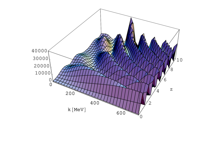
(a) The single pion momentum distribution as a function of the scaled time $z=\frac{1}{2}m_{\sigma}t$. The parameters are taken as $m_{\pi}$=140MeV, $m_{\sigma}$=600MeV, and $\chi_{0}/v=0.05$.

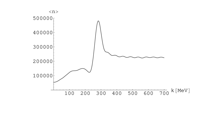
(b) The single pion momentum distribution integrated over time $z$ from 0 to 20, which corresponds to the period of time from $t=0$ to 13 fm.

REFERENCES

• [1] A. A. Anselm, Phys. Lett. B217 (1989) 169; A. A. Anselm and M. G. Ryskin, Phys. Lett. B266 (1991) 482; J. D. Bjorken, Acta Phys. Pol. B23 (1992) 561; J. D. Bjorken, K. L. Kowalski, and C. C. Taylor, Talk at 7th Rencontres de Physique de la Valee d’Aoste, La Thuile Rencontres 1993, page 507. J.-P. Blaizot and A. Krzywicki, Phys. Rev. D46 (1992) 246; Phys. Rev. D50 (1994) 442; K. Rajagopal and F. Wilczek, Nucl. Phys. B404 (1993) 577; S. Gavin, A. Gocksch, and R. D. Pisarski, Phys. Rev. Lett. 72 (1994) 2143; M. Asakawa, Z. Huang, and X.-N. Wang, Phys. Rev. Lett.74 (1995) 3126; K. Rajagopal, Talk at 25th International Workshop on Gross Properties of Nuclei and Nuclear Excitation: QCD Phase Transitions, January 13-18, 1997 Hirschegg, Austria, hep-ph/9703258.
• [2] L. T. Baradzei et al., Nucl. Phys. B370 (1992) 365. J. Lord and J. Iwai, paper submitted to International Conference on High Energy Physics, Dallas, Texas, 1992.
• [3] T. Brooks et al. (MiniMax Collaboration), hep-ph/9609375. J. Street, Talk at Argonne Workshop on Hadron Systems at High Density and/or High Temperature, August 7, 1997.
• [4] R. C. Hwa, Summary Talk at 7th International Workshop on Multiparticle Production; Correlations and Fluctuations, June 30-July 6, Nijmegen, Netherlands, in Multiparticle Physics 1996, page 377.
• [5] R. Hanbury-Brown and R. Q. Twiss, Phil. Mag. 45 (1954) 633; G. Goldhaber, S. Goldhaber, W. Lee, and A. Pais, Phys. Rev. 120 (1960) 300; E. V. Shuryak, Phys. Lett. B44 (1973) 387; Sov. J. Nucl. Phys. 18 (1974) 667; G. I Kopylov and M. I. Podgoretsky, Sov. J. Nucl. Phys. 14 (1971) 1084; 18 (1973) 656; G. I Kopylov, Phys. Lett. B50 (1974) 472.
• [6] C. Greiner, C. Gong, and B. Müller, Phys. Lett. B316 (1993) 226.
• [7] I. I. Kogan, JETP Lett. 59 (1994) 312; R. D. Amado and I. I. Kogan, Phys. Rev. D51 (1995) 190.
• [8] I. M. Dremin and R. C. Hwa, Phys. Rev. D53 (1996) 1216.
• [9] S. Mrówczyński and B. Müller, Phys. Lett. B363 (1995) 1.
• [10] Y. Shtanov, J. Traschen and R. Brandenberger, Phys. Rev. D51 (1995) 5438.
• [11] H. P. Yuen, Phys. Rev. A13 (1976) 2226; D. F. Walls, Nature 306 (1983) 141; D. F. Smirnov and A. S. Troshin, Sov. Phys. Usp. 30 (1987) 851.
• [12] L. Kofman, A. Linde, and A. A. Starobinsky, Phys. Rev. Lett. 73 (1994) 3195; Phys. Rev. D56 (1997) 3258.
• [13] D. Boyanovsky, H. J. de Vega, R. Holman, D.- S. Lee, and A. Singh, Phys. Rev. D51 (1995) 4419; D. Boyanovsky, H. J. de Vega, R. Holman, and J. F. J. Salgado, Phys. Rev. D54 (1996) 7570.
• [14] M. Yoshimura, Prog. Theor. Phys. 94 (1995) 873. H. Fujisaki et al., Phys. Rev. D53 (1996) 6805; D54 (1996) 2494.
• [15] M. Abramowitz and I. A. Stegun, Handbook of Mathematical Functions (Dover Publication, New York, 1965).
• [16] H. Hiro-Oka and H. Minakata, in preparation.
Refer to caption