The Mystery of Flavor

Abstract

After outlining some of the issues surrounding the flavor problem, I present three speculative ideas on the origin of families. In turn, families are conjectured to arise from an underlying preon dynamics; from random dynamics at very short distances; or as a result of compactification in higher dimensional theories. Examples and limitations of each of these speculative scenarios are discussed. The twin roles that family symmetries and GUTs can have on the spectrum of quarks and leptons is emphasized, along with the dominant role that the top mass is likely to play in the dynamics of mass generation.

I The Question of Flavor

Flavor is an old problem. I. I. Rabi’s famous question about the muon: “who ordered that?” has now been replaced by an equally difficult question to answer: “why do we have three families of quarks and leptons?” Although qualitatively we understand the issues connected to flavor a lot better now, quantitatively we are as puzzled as when the muon was discovered.

When thinking of flavor, it is useful to consider the standard model Lagrangian in a sequence of steps. At the roughest level, neglecting both gauge and Yukawa interactions, the Standard Model Lagrangian ${\cal{L}}_{o}={\cal{L}}_{\rm SM}(g_{i}=0;\Gamma_{ij}=0)$ has a $U(48)$ global symmetry corresponding to the freedom of being able to interchange any of the 16 fermions of the 3 families of quarks and leptons with one another. If we turn on the gauge interactions, the Lagrangian ${\cal{L}}_{1}={\cal{L}}_{\rm SM}(g_{i}\not=0;\Gamma_{ij}=0)$ has a much more restricted symmetry $[U(3))]^{6}$ corresponding to interchanging fermions of a given type (e.g. the $(u,d)_{\rm L}$ doublet) from one family to the other. When also the Yukawa interactions are turned on, ${\cal{L}}_{2}={\cal{L}}_{\rm SM}(g_{i}\not=0;\Gamma_{ij}\not=0)$, then the only remaining symmetry of the Lagrangian is $U(1)_{\rm B}\times U(1)_{\rm L}$. In fact, because of the chiral anomalyABJ , at the quantum level the symmetry of ${\cal{L}}_{2}$ is just $U(1)_{\rm B-L}$.

The above classification scheme serves to emphasize that there are really three distinct flavor problems. There is a matter problem , a family problem and a mass problem. The first of these problems is simply that of understanding the origin of the different species of quarks and leptons (i.e. why does one have a $\nu^{c}_{\rm L}$ and a $u^{c}_{\rm L}$ state?). The second problem is related to the triplication of the quarks and leptons. What physics forces such a triplication? Finally, the last problem is related to understanding the origin of the observed peculiar mass pattern of the known fermions.

The usual approach when thinking about flavor is to try to decouple the above three problems from one another. Thus, for example, one assumes the existence of the quarks and leptons in the Standard Model and asks for the physics behind the replication of families. Although it is difficult to argue cogently on this point, it is certainly true in the examples which we will discuss that the matter problem seems to be unrelated to the question of family replication. Indeed, quite often one also assumes the reverse, namely, that the family replication question is independent of the types of quarks and leptons one has. In fact, it is possible that there is other matter besides the known quarks and leptons and that this matter is also replicated. Certainly, even in the minimal Standard Model there is other matter besides the quarks and leptons, connected to the symmetry breaking sector. This raises a host of questions including that of possible family replication of the ordinary Higgs doublet. One knows, empirically, that this cannot happen if one is to avoid flavor changing neutral currents (FCNC)GW . However, some replication is needed if there is supersymmetry, but the two different Higgs doublets needed in supersymmetry are connected with different quark charges and need not replicate as families.

The above remarks suggests that there are some perils associated with trying to seek the origin for family replication independently from that of the quarks and leptons themselves. Nevertheless, that is the approach usually taken and the one I will follow here. Similarly, one also usually tries to disconnect the problem of mass from that of matter and family. That is, one generally assumes the existence of the three observed families of quarks and leptons, and then tries to postulate (approximate) symmetries of the mass matrices for quarks and leptons which will give interrelations among the masses and mixing parameters for some of these states.

This approach usually involves some kind of family symmetry and is sensible provided that:

i) There is some misalignment between the mass matrix basis and the gauge interaction basis for the quarks and leptons. Only through such a misalignment will there result a nontrivial mixing matrix: $V_{\rm CKM}\not=1$.

ii) The family symmetries of the mass matrices are broken (otherwise $V_{CKM}\equiv 1$) either explicitly or spontaneously. Furthermore, if the breaking is spontaneous, it must occur at a sufficiently high scale to have escaped detection so far.

Although the origin of flavor remains a mystery, I want to discuss here three speculative ideas for the origin of families. These ideas are realized up to now only in incomplete ways, in what amount essentially to toy models. Thus, for instance, the issue of family generation is in general disconnected from the question of $SU(2)\times U(1)$ breaking and, often, also from trying to explicitly calculate the Yukawa couplings. As a result, in all of these attempts at trying to understand flavor, the question of mass is approached from a much more phenomenological viewpoint. One guesses certain family or GUT symmetries, and their possible patterns of breaking, and then one checks out these guesses by testing their predictions experimentally. In all of these considerations, the top mass, because it is the dominant mass in the spectrum, plays a fundamental role.

In my lectures RDP , I will begin by describing three speculative ideas for the origin of families. Specifically, I will consider in turn the generation of families dynamically; through short distance chaotic dynamics; and as a result of geometry. After this speculative tour, I will discuss briefly the issue of mass generation. In particular, I will illustrate the twin roles that family symmetries and GUTs can have for the spectrum of quarks and leptons. I will conclude by commenting on the profound role that the top mass is likely to have on the detailed dynamics of mass generation.

II Generating Families Dynamically

The underlying idea behind this approach to the flavor problem is that familiies of quarks and leptons result because they are themselves composites of yet more fundamental ingredients–preons. There is a nice isotope analogyKLS which serves to illustrate this point. Think of the three isotopes of Hydrogen as three distinct families. Just like the families of quarks and leptons, all three isotopes have the same interactions–their chemistry being determined by the electromagnetic interactions of the proton. Deuterium and tritium, however, have different masses than the proton because they have, respectively, 1 and 2 neutrons. Of course, the analogy is not perfect since ${}^{1}H$ and ${}^{3}H$ are fermions and ${}^{2}H$ is a boson! Nevertheless, it is tempting to suppose that the 3 families of quarks and leptons, just like the Hydrogen isotopes, result from the presence of different “neutral” constituents.

I will illustrate how to generate families dynamically by using as an example some recent work of Kaplan, Lepeintre and SchmaltzKLS . By using essentially the isotope analogy, these authors constructed an interesting toy model of flavor. Their simplest toy model is based on an underlying supersymmetric gauge theory based on the symplectic group $Sp(6)$. The fundamental constituents in this model are 6 preons $Q_{\alpha}$ transforming according to the fundamental representation of $Sp(6)$ and one preon $A_{\alpha\beta}$ transforming according to the 2-rank antisymmetric representation. Such a theory has three families of bound states distinguished by their $A_{\alpha\beta}$ content, plus a pair of (neutral) exotic states. To wit, the bound states of the model are the 15 flavor states

$$F_{3}^{[i,j]}\sim Q^{i}_{\alpha}Q^{j}_{\alpha};~{}~{}F_{2}^{[i,j]}\sim Q^{i}_{\alpha}A_{\alpha\beta}Q_{\beta}^{j};~{}~{}F_{1}^{[i,j]}\sim Q^{i}_{\alpha}A_{\alpha\beta}A_{\beta\gamma}Q_{\gamma}^{j}$$ (1)

plus the two neutral exotic states

$$T_{2}\sim{\rm Tr}A^{2}~{};~{}~{}~{}T_{3}\sim{\rm Tr}A^{3}~{}.$$ (2)

The six $Q_{\alpha}$ preons act as the protons in the isotope analogy. In principle, one could imagine having the $SU(3)\times SU(2)\times U(1)$ interactions act on the $Q_{\alpha}$ states, while the $A_{\alpha\beta}$ preons act as the neutrons. Furthermore, there is clearly a family $U(1)_{\rm F}$ in the spectrum which counts the number of $A_{\alpha\beta}$ fields. Finally, one should note that, because of the supersymmetry, each of the states in Eqs. (1) and (2) contain both fermions and bosons.

Although the number of bound states per family (15) is encouraging, these states cannot really be the ordinary quarks and leptons (minus the right-handed neutrinos). It turns out that one cannot properly incorporate the $SU(3)\times SU(2)\times U(1)$ gauge interactions with only 6 $Q_{\alpha}$ preons. To do that, in fact, one has to at least triplicate the underlying gauge theoryKLS from $Sp(6)$ to $Sp(6)_{\rm L}\times Sp(6)_{\rm R}\times Sp(6)_{\rm H}$. Each of these $Sp(6)$ groups has again six $Q_{\alpha}$ and one $A_{\alpha\beta}$ preon. To obtain the desired quarks and leptons the $Q$ preons are assumed to have the following $SU(3)\times SU(2)\times U(1)$ assignments:

$$Q_{\rm L}: (3,1)_{0}\oplus(1,2)_{1/6}\oplus(1,1)_{-1/3}$$ (3)

$$Q_{\rm R}: (\bar{3},1)_{0}\oplus(1,1)_{-2/3}\oplus 2(1,1)_{1/3}$$

$$Q_{\rm H}: (1,2)_{-1/6}\oplus(1,1)_{1/3}\oplus(1,1)_{2/3}\oplus 2(1,1)_{-1/3}$$

Because of the preon group triplication, instead of having 15 $F^{[i,j]}$ bound states per family, one now has 45 such states. Per family, these states now include 16 states with the quantum numbers of the observed quarks and leptons, plus 29 exotic states which, however, sit in vector-like representations of the Standard Model group. Specifically, the quark doublet $(u,d)_{\rm L}$ is a bound state of $Sp(6)_{\rm L}$; $u^{c}_{\rm L}$ and $d^{c}_{\rm L}$ are bound states of $Sp(6)_{\rm R}$; while the lepton states $(\nu,e)_{\rm L}$, $\nu^{c}_{\rm L}$ and $e^{c}_{\rm L}$ are bound states of $Sp(6)_{\rm H}$. Among the exotic states one finds as bound states of $Sp(6)_{\rm H}$ two states with the quantum numbers of the Higgs doublets of a supersymmetric theory: $H_{1}\sim(h_{1}^{o},h_{1}^{-})$ and $H_{2}\sim(h_{2}^{+},h_{2}^{o})$. So, in this model, there is a natural family repetition of the Higgs states. Naively, this could cause problems with FCNC. It turns out, however, that when one calculates the dynamical superpotential of the theorySeiberg one can showKLS that there is a ground state where only one of the three families of Higgs states are left light. So, in fact, there are no FCNC problems.

This nice result is tempered by other troublesome features of the model which render it unrealistic–but not uninteresting. For example, to break the $[U_{\rm F}(1)]^{3}$ family symmetry of the model, it is necessary to introduce by hand some heavy fields (with masses $\mu>\Lambda$–the dynamical scale of the preon theories) which serve to couple the preon groups together. The simplest possibility is afforded by having 3 such fields: $v^{1}_{\alpha_{\rm H}\beta_{\rm R}},~{}v^{2}_{\alpha_{\rm R}\beta_{\rm L}},~{}v^{3}_{\alpha_{\rm L}\beta_{\rm H}}$ with indices spanning 2 of the preon groups, interacting through a superpotential

$$W = av^{1}v^{2}v^{3}+b^{1}_{\rm H}v^{1}v^{1}A_{\rm H}+b^{1}_{\rm R}v^{1}v^{1}A_{\rm R}+b^{2}_{\rm R}v^{2}v^{2}A_{\rm R}+b^{2}_{\rm L}v^{2}v^{2}A_{\rm L}$$ (4)

$$\mbox{}+b^{3}_{\rm L}v^{3}v^{3}A_{\rm L}+b^{3}_{\rm H}v^{3}v^{3}A_{\rm H}$$

The $a$-term above ties the preon theories together, while the various $b$-terms serve to break the family symmetries. Although Eq. (4) is introduced by hand, integrating out the effects of the heavy $v^{i}$ fields gives effective Yukawa couplings of different strengths, much in the way originally suggested by Froggatt and NielsenFN . This is illustrated schematically in Fig. 1 for the Yukawa coupling of $u^{c}_{\rm L}$ with $(c,s)_{\rm L}$ via the Higgs state $H^{(3)}_{2}$ of the third family–which is the only one which is assumed to get a VEV. One findsKLS

$$\Gamma^{(3)}_{12}\sim a~{}b_{\rm R}^{1}b_{\rm R}^{2}b_{\rm L}^{3}(\Lambda/\mu)^{6}\sim\epsilon^{6}$$ (5)

Although the various elements in the up-and-down quark mass matrices are hierarchial, unfortunately there is no resulting quark mixing since $M_{u}\sim M_{d}$. This follows because the model has an unbroken global $SU(2)$ symmetry at the preon level corresponding to the interchange of the $(1,1)_{-2/3}$ and $(1,1)_{1/3}$ assignments in Eq. (3). Furthermore, for the lepton sectors there is a dynamically generated set of Yukawa couplingsSeiberg which are typically unsuppressed. As a result, naively, one expects $m_{\tau}\gg m_{t}$. Both of these results make the $[Sp(6)]^{3}$ model as presented above unrealistic. By further complicating the model, Kaplan, Lepeintre and SchmaltzKLS are able to obtain both a non-trivial CKM matrix and re-establish the top as the heaviest bound state. However, these “improved” models are not particularly attractive and represent, more than anything else, a “proof of principle”. In addition, even after these problems are resolved, the models still lack mechanisms for breaking $SU(2)\times U(1)$ and supersymmetry, features which must be understood to make contact with reality.

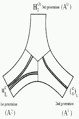
Figure 1: Effective Yukawa coupling generated in the $[Sp(6)]^{3}$ preon model.

These negative remarks should not obscure the considerable achievement of these dynamical models for understanding the origin of flavor. Families in these models arise as a result of hidden degrees of freedom in some underlying confining dynamics. Furthermore, the presence of heavy excitations in this same dynamics can result in hierarchial patterns of Yukawa couplings, once all family symmetries are explicitly broken. Unfortunately, it is difficult to see how one can obtain real evidence for these kinds of schemes, barring the discovery of some of the exotic bound states they predict–in the example discussed, the $T_{2}$ and $T_{3}$ states or the vector-like partners of the quarks and leptons.

III Families from Short-Distance Random Dynamics

A radically different scheme for the origin of families has been proposed and elaborated by Holgar Nielsen and his collaboratorsRD . The basic idea that Nielsen has put forth is that there exist both order and chaos at very short distances. He imagines that at scales much smaller than the inverse of the Planck mass there is actually a lattice structure of scale length $a\ll 1/M_{\rm Planck}$. However, both the dynamics on the lattice as well as the structure of the lattice is random. In particular, the lattice is amorphous with sites at random positions. Furthermore, characteristic of the random dynamics, the interactions on each of the links are governed by different groups, with the groups varying from link to link.

Remarkably, even starting from these very general assumptions, one can arrive at some conclusions. Generally, one naively would imagine that no group could survive the random dynamics. That is, that the gauge group will end up by breaking down spontaneously, producing supermassive fields of mass $M\sim a^{-1}\gg M_{\rm Planck}$. In fact, as Brene and NielsenBN showed, there are special groups $G_{\rm surv.}$ on the links which survive the random dynamics–i.e., the associated vector bosons are massless. What Brene and NielsenBN showed is that the groups which survive must have a center which is non-trivial and connected. By taking values in the center the links are effectively gauge-invariant. However, the center cannot be simply the unit matrix because the random nature of the dynamics would then end up by averaging out the effects of all links. The connectedness of the center, finally, is necessary to insure that the Bianchi identities are satisfied. Specifically, it turns out that $G_{\rm surv.}$ is a product of “prime” groups with a certain discrete group $D_{\rm prime}$, generated from the center, removed:

$$G_{\rm surv.}=U(1)\times SU(2)\times SU(3)\times SU(5)\times~{}\ldots~{}SU(\rm prime)/D_{\rm prime}$$ (6)

From the above, it appears that Nielsen’s random dynamics allows the Standard Model group to survive, with a restriction:

$$G^{*}_{\rm SM}=SU(3)\times SU(2)\times U(1)/D_{3}~{}.$$ (7)

Here the discrete group $D_{3}$ is given by powers of the center element $h=\left\{e^{\frac{2\pi i}{3}}I_{3},-I_{2},e^{\frac{2\pi i}{6}}\right\}$:

$$D_{3}=\left\{h^{n}|n\subset Z_{6}\right\}$$ (8)

In practice, this imposes a restriction on the matter states which are placed on the random lattice sites

$$h\psi=\psi~{},$$ (9)

which fixes the hypercharge of the quarks relative to the leptons. Eq. (9) effectively imposes the familiar charge quantization, giving the quarks third-integral charges. This is a very nice result!

In this scheme the origin of family replication occurs through what Bennett, Nielsen and PicekBNP call “confusion” in the random dynamic processes. This can be understood as follows. At some step in the random dynamics what survives is not simply the group $G^{*}_{\rm SM}$ but a number $N_{\rm F}$ of copies of $G^{*}_{\rm SM}$, each with one family of quarks and leptons. Subsequently, this product group collapses to its diagonal subgroup $[G^{*}_{\rm SM}]_{\rm diag}$. This collapse, through “confusion”, results in $N_{\rm F}$ replicas of a Standard Model family of quarks and leptons. Thus, schematically, family generation occurs in random dynamics when $N_{\rm F}$ Standard Model surviving groups collapse:

$$G^{*}_{\rm SM}\times G^{*}_{\rm SM}\times~{}\ldots~{}\times G^{*}_{\rm SM}\to[G^{*}_{\rm SM}]_{\rm diag}$$ (10)

Bennett, Nielsen and PicekBNP try to estimate $N_{\rm F}$–the number of families–which arise from random dynamics confusion by making a number of assumptions. Although some of these assumptions are questionable, they are not unreasonable. First, Bennett et al. suppose that the lattice scale associated with the random dynamics is of order of the Planck scale: $a=M_{\rm P}^{-1}$. This allows the calculation of the coupling constants of the Standard Model group $[G^{*}_{\rm SM}]_{\rm diag}$ from their low energy values via the renormalization group:

$$[g_{i}]_{\rm diag}\simeq g_{i}[M_{\rm P}]$$ (11)

Second, by identifying the gauge fields in $[G^{*}_{\rm SM}]_{\rm diag}$ with the individual fields in each of the SM groups in Eq. (10), it follows that the individual couplings of each of the groups in the “confused” configuration $G^{*}_{\rm SM}\times G^{*}_{\rm SM}\times~{}\ldots~{}\times G^{*}_{\rm SM}$ is given by

$$g_{i}^{\rm conf}=\sqrt{N_{\rm F}}[g_{i}]_{\rm diag}$$ (12)

A knowledge of $g_{i}^{\rm conf}$ then provides an estimate for $N_{\rm F}$. What Bennett, Nielsen and PicekBNP assume is that

$$g_{i}^{\rm conf}=g_{i}^{*}~{},$$ (13)

with $g_{i}^{*}$ being the mean field theory critical coupling for each of the groups in the Standard Model. This assumption guarantees that in the confusion stage there is no confinement of quark and lepton states at Planck length scales–a reasonable boundary condition.

The result for $N_{\rm F}$ which follows from the three assumptions (11)-(13) are rather remarkable, given the spare theoretical framework! One findsRD

$$N_{\rm F}=\left\{\begin{array}[]{ll}3.4&{\rm U(1)}\\ 3.5&{\rm SU(2)}\\ 3.1&{\rm SU(3)}\end{array}\right.$$ (14)

This result notwithstanding, however, it is not clear how one proceeds further in developing a consistent theoretical framework from random dynamics. For instance, it is totally unclear how through this scheme one induces the breakdown of the $SU(2)\times U(1)$ electroweak group at scales of $O(100~{}{\rm GeV})$, or how one even generates the Yukawa couplings which can provide the quarks and leptons eventually with some mass.

IV A Geometrical Origin for Families

Perhaps the most interesting way to get family replications is through the compactification of extra dimensions. One starts with a theory in $d>4$ dimensions but then assumes that the extra dimensions somehow compactify, leaving a 4-dimensional theory. The earliest example of such a theory was the 5-dimensional Kaluza-Klein theory of gravityKK , which when compactified to 4 dimensions gave rise, in addition to gravity, also to electromagnetic interactions. More modern examples are superstring theoriesGSW which are known to be consistent only in $d>4$ dimensions, but where again the extra dimensions can compactify leaving an effective 4-dimensional theory.

It is quite easy to understand how one can generate families in these types of theories. The general idea was first sketched out by WetterichWetterich and WittenWitten in the early 1980’s. Consider chiral fermions in a d-dimensional space-time. Such fermions, by definition, obey a massless Dirac equation

$$\Gamma^{\alpha}D_{\alpha}\psi=0$$ (15)

Here $\alpha=1,2,\ldots d$ and $D_{\alpha}$ is the Dirac operator in the background of whatever other fields (gravity, Yang-Mills) are present in the theory. Suppose now ($d-4$) dimensions compactify. Then Eq. (15) can be written as

$$(\Gamma^{\mu}D_{\mu}+\Gamma^{a}D_{a})\psi=0$$ (16)

with $\mu=0,1,2,3$ and $a=4,~{}\ldots~{},~{}d-1$. Clearly the ($d-4$) operator $\Gamma^{a}D_{a}$ in Eq. (16) acts as a 4-dimensional mass $[\Gamma^{a}D_{a}\equiv M]$ unless it vanishes when applied on $\psi$:

$$\Gamma_{a}D^{a}\psi=0$$ (17)

If Eq. (17) holds, corresponding to a chirality constraint on the ($d-4$)-dimensional compact space $K$, then also the 4-dimensional fermions will be chiral. If (17) does not hold, then the resulting 4-dimensional fermions have a mass.

Since the quarks and leptons are chiral, if they are produced from $d>4$ chiral fermions via compactification of the extra dimension, a constraint equation like (17) on the compact space $K$ must hold. Now, in general, such constraint equations have a number of solutions, which depend on the intrinsic properties of the compact space $K$. So, in these kinds of theories, families and family number are intrinsically related to the topological properties of compact spaces associated with the original $d>4$ theory.

Perhaps the best known example of family replication using these ideas is the one considered by Candelas, Horowitz, Strominger, and WittenCHSW involving the Calabi-Yau compactification of the $d=10$ heterotic superstring. This string theoryheterotic has an associated $E_{8}\times E_{8}$ gauge symmetry and is supersymmetric. The chiral fermions in the $d=10$ theory are gauginos of one of the $E_{8}$ groups (the other $E_{8}$ acts as a hidden sector), sitting in the 248 dimensional adjoint representation. Candelas et al.CHSW assumes that the 10-dimensional space of the theory compactifies down to $d=4$ Minkowski space times a 6-dimensional Calabi-Yau space, whose principal property for our purposes is that it possesses an $SU(3)$ holonomy. This means that the chiral zero modes in $K$–those that obey the constraint equations (17)–have non-trivial $SU(3)$ properties, even though this $SU(3)$ is broken in the compactification. By decomposing $E_{8}$ into its $E_{6}\times SU(3)$ subgroup one identifies the chiral zero modes in the gauginos which are candidates for the surviving chiral matter in 4 dimensions. Since, under this decomposition,

$$248=(78,1)\oplus(27,3)\oplus(2\bar{7},\bar{3})+(1,8)$$ (18)

one sees that, after Calabi-Yau compactification, the 4-dimensional chiral matter involve fermions in either the 27 or $2\bar{7}$ reprentations of $E_{6}$. So, in general, one expects to have $n_{\rm F}$ 27 plus $\delta(27+2\bar{7})$ states in the spectrum. The numbers $n_{\rm F}$ and $\delta$ are related to topological indices characteristic of the Calabi-Yau space $K$ which compactified. In particular, Candelas et al.CHSW showed that $n_{\rm F}$–the number of families–is connected to the Euler number of $K$:

$$n_{\rm F}=\frac{1}{2}~{}n_{\rm Euler}$$ (19)

Note that, in this example, the families one obtains have the right stuff. The 27-dimensional representation of $E_{6}$ when decomposed in terms of its $SO(10)$ subgroup contains the 16-dimensional representation, appropriate for a family of quarks and leptons, plus a 10 and a singlet. The 10 itself, since the theory is supersymmetric, contains the two needed Higgs doublets, which in this case also come in family repetitions. In principle, the $\delta(27+2\bar{7})$ states (as well as the 10 and 1) are vectorlike, and one can imagine these states getting masses of the order of the compactification scale–presumably of $O(M_{\rm P})$. So in this example, the light states are just $n_{\rm F}$ replications of the chiral quarks and leptons!

Connecting family replication to the geometry of a compact space is a beautiful idea. Furthermore, there is another advantage. Through compactification, Yukawa couplings are naturally produced, arising from the fermion-gauge field interactions in $d>4$ dimension along the gauge field components in the $(d-4)$ compact dimensions. Unfortunately, however, one cannot in general compute these couplings explicitly. Nevertheless, often one can infer some useful symmetry restrictions among the Yukawa couplings in these schemesGKR .

In my view, obtaining families from compactification is the most appealing solution to the origin of the mysterious repetitions we see in nature. It is not, however, easy to arrive at the correct theory. Basically, even believing that superstrings are the right theory, we still do not understand how to choose among the many possible compactifications available for these theories, since we have no idea of what is the underlying physics principle that drives the compactification. At the same time, we are also ignorant of how these schemes can give rise to terms which break supersymmetry and eventually $SU(2)\times U(1)$. Until such problems are solved, these ideas will just remain ideas which are appealing but untested.

V Navigating through the Mass Maze

Even if one were to eventually understand the origin for families and their matter content, the mystery of flavor will not be solved until one is able also to decipher the physics which leads to the peculiar mass spectrum of quarks and leptons. Lacking a complete theory, most physicists have taken a very pragmatic approach to the mass generation problem. Basically, what has been assumed is that this problem is essentially decoupled from that of families and matter. Therefore, it makes sense to pursue a quite phenomenological strategy to get some insights into the problem of mass.

Following the lead set by some early work of WeinbergWeinberg and FritzschFritzsch , the strategy has been to assume that the mass matrices for the fermions have certain “textures”, imposed on them by some underlying symmetries. These textures, in turn, allow one to derive some interesting “predictions” which can then be compared with experiment. Typically, one obtains in this way certain interrelations among the quark mixing angles and the quark masses–relations which go beyond the standard model.

Perhaps the most famous “prediction” of this type of approach is the following formula for the Cabibbo angle, expressed as a function of quark mass ratios:

$$\sin\theta_{c}=\sqrt{\frac{m_{d}}{m_{s}}}-\sqrt{\frac{m_{u}}{m_{c}}}$$ (20)

Equation (20) follows directly, in the case of two generations, if the quark mass matrices have the Fritzsch patternFritzsch

$$M_{u}=\left(\begin{array}[]{cc}O&A\\ A&B\end{array}\right)~{};~{}~{}~{}~{}M_{D}=\left(\begin{array}[]{cc}O&C\\ C&D\end{array}\right)$$ (21)

which display a texture zero in the 11 matrix element. Given that Eq. (20) is rather successful phenomenologically, the natural question to ask in this context is the underlying reason for the appearance of the texture zero in Eq. (21).

The appearance of texture zero or other interrelations between the elements in the quark and lepton mass matrices are generally assumed to arise at some high scale $M$ where new physics connected with mass generation comes into play. In models where the breakdown of $SU(2)\times U(1)$ is dynamical like TechnicolorTC , the scale $M$ is generally assumed to be not too far from the TeV scale. However, in general, one has to be careful with FCNC induced through the process of mass generationDE and one must appeal to dynamical properties of the underlying theoryWTC to avoid contradiction with experiment. The resulting theories are quite complicatedHoldom and, as a result, many physicists think it more likely that the scale $M$ connected with mass generation is likely to be of order of the Planck or GUT scale. In what follows, I shall concentrate only on this latter possibility and discuss two different, but complementary, mechanisms which can provide mass matrices with interesting textures: family symmetries and GUTs.

I will illustrate the first of these possibilities by discussing briefly a model introduced by Ibañez and RossIR , which makes use of a $U(1)_{\rm F}$ family symmetry. In the Ibañez-Ross model, the quarks and antiquarks of each generation have the opposite $U(1)_{\rm F}$ charge, while the two Higgs bosons $H_{1}$ and $H_{2}$ of the model carry twice the $U(1)_{\rm F}$ charge of the third generation:

$$\left(\begin{array}[c]{c}u\\ d\end{array}\right)^{i}_{\rm L}\to e^{i\alpha_{i}}\left(\begin{array}[]{c}u\\ d\end{array}\right)^{i}_{\rm L};\begin{array}[c]{c}\left(u^{c}_{L}\right)^{i}\to e^{-i\alpha_{i}}\left(u^{c}_{L}\right)^{i}\\ \left(d^{c}_{L}\right)^{i}\to e^{-i\alpha_{i}}\left(d^{c}_{L}\right)^{i}\end{array};\begin{array}[c]{c}H_{1}\to e^{2i\alpha_{3}}H_{1}\\ H_{2}\to e^{2i\alpha_{3}}H_{2}\end{array}$$ (22)

As a result of this symmetry, clearly the quark mass matrices only have a non-zero 33 element:

$$M_{\rm 0}^{u,d}=m_{t,b}\left(\begin{array}[]{ccc}0&0&0\\ 0&0&0\\ 0&0&1\end{array}\right)$$ (23)

This provides a reasonable starting point for model building.

To proceed, Ibañez and RossIR need to introduce both a way to break the $U(1)_{\rm F}$ symmetry and some interactions which physically will serve to generate the integenerational mass splittings. They accomplish the second point by imagining that at some high scale $M$ some $SU(2)\times U(1)$ singlet fields $\theta$ and $\bar{\theta}$, with $U(1)_{\rm F}$ charges of +1 and -1, respectively, acquire some effective interactions with the quark and Higgs fields. How these effective interactions come about need not be specified, but the $U(1)_{\rm F}$ symmetry will fix their form. Ibañez and Ross essentially make use of the Froggatt-NielsenFN mechanism we illustrated earlier with the $[Sp(6)]^{3}$ preon model. For example, there will be a $U(1)_{\rm F}$ preserving effective interaction among the $u$ and $t$ quarks and the two scalar fields $H_{2}$ and $\theta$ of the form

$${\cal{L}}_{ut}^{\rm eff}\sim\left(\frac{\theta}{M}\right)^{\alpha_{1}-\alpha_{3}}~{}~{}\bar{u}_{\rm L}H_{2}t_{\rm L}^{c}$$ (24)

Ibañez and RossIR , in addition, assume that the $U(1)_{\rm F}$ family symmetry is itself spontaneously broken at high scales by VEVs of the $\theta$ and $\bar{\theta}$ fields. Once $\theta$ acquires a VEV a term like (24) becomes an effective Yukawa interaction, which can give rise to small corrections to the mass matrix (23) if $\epsilon=\frac{\langle\theta\rangle}{M}\ll 1$. Of course, within this approach, one is not able to predict precisely these corrections. Nevertheless, if one assumes that the proportionality constants in the Froggatt-Nielsen terms are of $O(1)$, the magnitude of the different matrix elements will be governed by powers of $\epsilon$, reflecting the original $U(1)_{\rm F}$ symmetry. In the case of the Ibañez and Ross model, for example, the modified up-quark mass matrix under these assumptions takes the form

$$M_{1}^{u}\sim m_{t}\left(\begin{array}[]{ccc}\epsilon^{|-4\alpha_{1}-2\alpha_{2}|}&\epsilon^{|-3\alpha_{1}|}&\epsilon^{|-\alpha_{2}-2\alpha_{1}|}\\ \epsilon^{|-3\alpha_{1}|}&\epsilon^{2|\alpha_{2}-\alpha_{1}|}&\epsilon^{|\alpha_{2}-\alpha_{1}|}\\ \epsilon^{|-\alpha_{2}-2\alpha_{1}|}&\epsilon^{|\alpha_{2}-\alpha_{1}|}&1\end{array}\right)$$ (25)

Not only is this mass matrix hierarchial if $\epsilon\ll 1$, but there are interesting interrelations among the matrix elements; for example

$$(M_{1}^{u})_{11}\simeq\frac{\left[(M_{1}^{u})^{2}_{13}\right]^{2}}{(M_{1}^{u})_{33}}~{};~{}~{}~{}~{}(M_{1}^{u})_{22}\simeq\frac{\left[(M_{1}^{u})_{23}\right]^{2}}{(M_{1}^{u})_{33}}$$ (26)

In general, the detailed comparison of a mass matrix like that in Eq. (25), which holds at a large scale $M$, with experiment is complicated by the evolution of the Yukawa couplings with energy. This evolution, for example, can change zeros in a mass matrix at a given scale into small, but non-vanishing, contributions at a different scale. This is easy to understand since, for example, a non-vanishing Yukawa coupling to quarks of the second generation can induce at one loop an effective Yukawa coupling to quarks of the first generation, provided there is also a non-vanishing Yukawa coupling between the first two generations.

The effect of the renormalization group evolution of the couplings is to further obscure possible mass matrix patterns. For instance, the mass matrix $M^{u}$ of Eq. (25) is connected to the Yukawa couplings $\Gamma_{u}$ via the familiar equation $M^{u}=\frac{\Gamma_{u}}{\sqrt{2}}\langle H_{2}\rangle$. However, $\Gamma_{u}$ at one scale is different from $\Gamma_{u}$ at another scale, with the evolution between scales governed by the renormalization group. At one loop, this evolution is given by the equation:

$$16\pi^{2}\frac{d\Gamma_{u}}{d\ln M/\mu}= \left\{{\rm Tr}~{}(3\Gamma_{u}\Gamma_{u}^{\dagger}+3a\Gamma_{d}\Gamma_{d}^{\dagger}+a\Gamma_{\ell}\Gamma_{\ell}^{\dagger})\right.$$ (27)

$$\left.-G_{u}^{2}+\frac{3}{2}(b\Gamma_{u}\Gamma_{u}^{\dagger}+c\Gamma_{d}\Gamma_{d}^{\dagger})\right\}\Gamma_{u}$$

In the above, the coefficients $a,b,c$ and $G_{u}^{2}$ depend on the assumptions one makes on the matter content between the scale $M$ and the scale $\mu$. As a result, patterns set by physics at a high scale $M\sim O(M_{\rm Planck})$ at lower energies $\mu$ are smudged. In particular, the measured mass matrix at $\mu\sim M_{\rm Z}$ is influenced by the assumptions one makes on the matter content in the region between $\mu$ and $M$–a region for which one has no information! Nevertheless, once one fixes this matter content through some model assumptions, one can either validate or exclude specific mass matrix models by comparing their, renormalization group evolved, predictions with precision electroweak data.

Rather than illustrating this for the model of Ibañez and Ross sketched above, I prefer instead to examine the predictions of a specific class of SUSY GUT models, based on $SO(10)$ studied by Anderson, Dimopoulos, Hall, Raby and StarkmanADHRS . These models illustrate a second way in which theoretical input at a high scale may help fix the patterns of the quark and lepton masses and mixing we observe. These SUSY $SO(10)$ models have texture zeros and matrix element interrelations set by $SO(10)$, with hierarchies among these elements produced by insertion of higher dimensional operators much along the lines of what transpired in the Ibañez and Ross model. The best model of ADHRS with three texture zeros has the following Yukawa couplings:

$$\Gamma_{u} = \left(\begin{array}[]{ccc}0&C&0\\ C&0&-\frac{B}{3}\\ 0&-\frac{4B}{3}&A\end{array}\right)~{};~{}~{}~{}~{}\Gamma_{d}=\left(\begin{array}[]{ccc}0&-27C&0\\ -27C&Ee^{i\phi}&\frac{B}{9}\\ 0&-\frac{4B}{9}&A\end{array}\right)~{};$$ (34)

$$\Gamma_{\ell} = \left(\begin{array}[]{ccc}0&-27C&0\\ -27C&3Ee^{i\phi}&B\\ 0&2B&A\end{array}\right)$$ (38)

The parameters $A,B,C$ and $E$ have the following hierarchy

$$A\gg B\gg E>C$$ (39)

and the model Clebsch-Gordan coefficients have a Georgi-JarlskogGJ pattern for $\Gamma_{22}:~{}[u;d;\ell]=[0;1;3]$, which produces the nice result

$$\frac{m_{s}}{m_{d}}\simeq\frac{m_{\mu}}{9m_{e}}$$ (40)

Although these and other results provide an acceptable fit to the low-energy data, a recent analysis by Blacek, Carena, Raby and WagnerBCRW has shown that these models do not fit the data as well as models with just one texture zero, like the Lucas-Raby modelLR .

The Lucas-Raby model adds two non-zero matrix elements to the Yukawa coupling of Eq. (28), with strength $D\sim O(C)$. Specifically one has:

$$(\Gamma_{u})_{13}=-\frac{4D}{3}e^{i\delta}~{}~{} ;(\Gamma_{u})_{31}=-\frac{D}{3}e^{i\delta}~{}~{} ;(\Gamma_{d})_{13}=\frac{2D}{3}e^{i\delta}~{}~{};$$

$$(\Gamma_{d})_{31}=-9De^{i\delta}~{}~{} ;(\Gamma_{\ell})_{13}=-54De^{i\delta}~{}~{} ;(\Gamma_{\ell})_{31}=-De^{i\delta}$$ (41)

Table 1 displays a comparison of the fits provided by these two models of all the extant low-energy data. As can be seen, perhaps not surprisingly, the data clearly favors the Lucas-Raby model with all predictions within one standard deviation from the data. In contrast, the best of the Anderson et al.ADHRS models has four observables about $3\sigma$ away from the data:

Observable	Central Value	$\sigma$		Result ofADHRS		Result ofLR
$M_{\tau}$	175.0	6.0		173.9		175.7
$m_{b}(M_{t})$	4.26	0.11		4.360		4.287
$M_{b}-M_{c}$	3.4	0.2		3.146		3.440
$m_{s}$	180	50		162.6		189.0
$m_{d}/m_{s}$	0.05	0.015		0.0461		0.0502
$Q^{-2}$	0.00203	0.00020		0.00173		0.00204
$M_{\tau}$	1.777	0.0089		1.777		1.776
$M_{\mu}$	105.66	0.53		105.6		105.7
$M_{e}$	0.5110	0.0026		0.5113		0.5110
$V_{us}$	0.2205	0.0026		0.2215		0.2205
$V_{cb}$	0.0392	0.003		0.0450		0.0400
$V_{ub}/V_{cb}$	0.08	0.02		0.0463		0.0772
$B_{K}$	0.8	0.1		0.9450		0.8140

Table 1: Comparison of the Models of Ref.ADHRS and Ref.LR with Experiment: Adapted fromBCRW

$Q^{-2}=\frac{m_{d}^{2}-m_{u}^{2}}{m_{s}^{2}}~{};~{}~{}~{}V_{cb}~{};~{}~{}V_{ub}/V_{cd}~{}~{}\hbox{and}~{}~{}\hat{B}_{K}$ –the parameter characterizing the strength of the $K^{o}-\bar{K}^{o}$ matrix element which enters in the CP violating $\epsilon$ parameter.

I should remark that, besides fitting the extant data, these models are predictive. Once all the parameters (A-E and the phases) in Eqs. (28) and (31) are fixed from the global fit, one can extract further information from these ansatze, both on the CKM matrix as well as on the spectrum of Higgs and supersymmetric states. For example, the Lucas-Raby model predicts the following values for the parameters associated with the CKM unitary triangle, so important for studies of CP violation in the B systemLR .

$$\sin 2\alpha=0.96~{};~{}~{}\sin 2\beta=0.52~{};~{}~{}~{}\sin\gamma=0.93~{};\rho=-0.125~{};~{}~{}~{}\eta=0.32$$ (42)

The angles $\alpha,\beta$ and $\gamma$ will be soon measured and Eq. (32) will be tested experimentally. At the same time, the Lucas-Raby model also predicts that the lightest Higgs bosons are a pair of CP odd and CP even states nearly degenerate with each other with mass around 74 GeV–a prediction which should be tested already by LEP 200.

VI Lessons from the Top Mass.

Because $m_{t}\gg m_{i}$, many of the important features of the Yukawa matrices are crucially dependent on how the top coupling behaves. Theoretically, rather than considering the physical mass for the top measured by the CDF and DO CollaborationsPDG $M_{t}=(175\pm 6)$ GeV, it is more useful to consider the running mass

$$m_{t}(M_{t})\sim\frac{M_{t}}{1+\frac{4}{3\pi}\alpha_{s}(m_{t})}=(167\pm 6)~{}{\rm GeV}$$ (43)

The running mass is directly related to the diagonal Yukawa coupling of the top $\lambda_{t}(m_{t})$

$$m_{t}(m_{t})=\lambda_{t}(m_{1})\langle H_{2}\rangle$$ (44)

This coupling, keeping only the dominant 3rd generation couplings in Eq. (27) obeys the RG equationOP

$$\frac{d\lambda_{t}(\mu)}{d\ln\mu}=\frac{1}{(4\pi)^{2}}\left\{a_{t}\lambda_{t}^{2}(\mu)+a_{b}\lambda_{b}^{2}(\mu)+a_{\tau}\lambda_{\tau}^{2}(\mu)-4\pi c_{i}\alpha_{i}(\mu)\right\}\lambda_{t}(\mu)$$ (45)

The coefficients $a_{i},c_{i}$, as we discussed earlier, depend on the matter content of the theory. For instance, for the SM one has

$$a_{t}=\frac{9}{2}~{};~{}~{}a_{b}=\frac{3}{2}~{};~{}~{}a_{\tau}=1~{};~{}~{}c_{i}=\left(\frac{17}{20}~{};~{}~{}\frac{9}{4}~{};~{}~{}8\right)~{},$$ (46)

while for the minimal supersymmetric extension of the Standard Model (MSSM) one has

$$a_{t}=6~{};~{}~{}a_{b}=1~{};~{}~{}a_{\tau}=0~{};~{}~{}c_{i}=\left(\frac{13}{5}~{};~{}~{}3~{};~{}~{}\frac{16}{3}\right)$$ (47)

Knowing the value for $\lambda_{t}(m_{t})$ one can compute the value for $\lambda_{t}(\mu)$ at any scale $\mu$ by using the RG equation (35). Because $a_{t}>0$, for $\mu$ large enough eventually $\lambda_{t}(\mu)\to\infty$. The location of this, so called, Landau poleLandau is theory-dependent. As we shall see, $\mu_{\rm Landau}$ is an uninteresting scale in the SM, but for the MSSM $\mu_{\rm Landau}\sim M_{\rm Planck}$–a result which may be quite significant. At any rate, it is worthwhile to explore these differences in a bit more detailSW .

For the Standard Model, because one has only one Higgs boson, one has $\langle H_{2}\rangle\equiv\langle H\rangle\simeq\frac{1}{2^{3/4}G_{F}^{1/2}}\simeq 174~{}{\rm GeV}$ and $\lambda_{t}(m_{t})=0.96\pm 0.04$. Furthermore, in this case, because top is so heavy $\lambda_{t}^{2}\gg\lambda_{b}^{2}~{},~{}\lambda_{\tau}^{2}$ and these other couplings can be safely dropped from Eq. (35). The solution of the RG equation

$$\frac{d\lambda_{t}(\mu)}{d\ln\mu}=\frac{1}{(4\pi)^{2}}\left\{a_{t}\lambda_{t}^{2}(\mu)-4\pi c_{i}\alpha_{i}(\mu)\right\}\lambda_{t}(\mu)$$ (48)

is easily found to be

$$\lambda_{t}^{2}(\mu)=\frac{\eta(\mu)\lambda_{t}^{2}(m_{t})}{\left[1-\frac{a_{t}}{8\pi^{2}}\lambda^{2}_{t}(m_{t})I(\mu)\right]}~{}.$$ (49)

Here $\eta(\mu)$ and $I(\mu)$ are functions determined by the running of the gauge coupling constants

$$\frac{d\alpha_{i}(\mu)}{d\ln\mu}=\frac{b_{i}}{2\pi}\alpha_{i}^{2}(\mu)$$ (50)

with $b_{i}\equiv\left(\frac{41}{10}~{},~{}~{}-\frac{19}{6}~{},~{}~{}-7\right)$ and one finds

$$\eta(\mu)=\Pi_{i}\left[\frac{\alpha_{i}(m_{t})}{\alpha_{i}(\mu)}\right]^{c_{i}/b_{i}}~{};I(\mu)=\int^{\ln(\mu)}_{\ln(m_{t})}\eta(\mu^{\prime})d\ln\mu^{\prime}.$$ (51)

From Eq (39) one sees that the Landau pole for the SM model occurs at a value of $\mu$ where

$$I(\mu_{\rm Landau})\biggr{|}_{\rm SM}=\frac{8\pi^{2}}{a_{t}\lambda_{t}^{2}(m_{t})}\simeq 18.9$$ (52)

Using Eq. (36) one finds $\mu_{\rm Landau}\simeq 10^{32}$ GeV a scale well beyond the Planck mass, which has clearly no physical significance. At the Planck mass, $I(M_{\rm Planck})\sim 12.2$, so one is still far away from the Landau pole. Indeed $\lambda_{t}(M_{\rm Planck})\sim 0.7<\lambda_{t}(m_{t})$. So the top Yukawa coupling in the SM remains perturbative $(\lambda_{t}^{2}/4\pi\ll 1)$ up to the Planck scale.

The situation is quite different if there is supersymmetry. Because there are now two Higgs doublets, $\lambda_{t}(m_{t})$ is not fixed by $m_{t}(m_{t})$ but depends also on the ratio of the two Higgs VEV, $\tan\beta$. One has $\langle H_{2}\rangle=\frac{1}{2^{3/4}G_{F}^{1/2}}\sin\beta$, so that

$$\lambda_{t}(m_{t})=\frac{0.96\pm 0.04}{\sin\beta}$$ (53)

There are two interesting regions for $\tan\beta$. The first of these has $\tan\beta\sim O(1)$, in which case one can again neglect $\lambda_{b}$ with respect to $\lambda_{t}$ in Eq. (35). In the second region $\tan\beta\gg 1$, but $\lambda_{t}(m_{t})\simeq\lambda_{b}(m_{t})$. That is, there is a unification of the top and bottom Yukawa couplings. In either of these two regions Eq. (35) reduces to the same approximate form (38). However, now one has either

$$a_{t}=6~{};~{}~{}~{}\lambda_{t}(m_{t})=\frac{0.96\pm 0.04}{\sin\beta}$$ (54)

if $\tan\beta\sim O(1)$. If $\tan\beta\gg 1$ instead, one has

$$a_{t}=7~{};~{}~{}~{}\lambda_{t}(m_{t})=0.96\pm 0.04$$ (55)

The form of the solution for $\lambda_{t}^{2}(\mu)$ in these two cases is again given by Eq. (39). However, here the running of the gauge couplings which enter in $\eta(\mu)$ and $I(\mu)$ is governed by a different set of coefficients $b_{i}$ and $c_{i}$, appropriate to having supersymmetric matter above the weak scale. In particular, $b_{i}=\left(\frac{33}{5}~{},~{}~{}1~{},~{}~{}-3\right)$. Given Eqs. (44) and (45), it is clear that the Landau pole will occur at the same place in both cases, provided that in the first case $\sin\beta=\sqrt{\frac{6}{7}}~{}(\tan\beta\simeq 2.45)$. In what follows, therefore, we concentrate only on the second case, corresponding to Yukawa unification of couplings.

The Landau pole in this case occurs at

$$I(\mu_{\rm Landau})\biggr{|}_{\rm MSSM}=\frac{8\pi^{2}}{a\lambda^{2}_{t}(m_{t})}=12.15\pm 1.00$$ (56)

Using the MSSM coupling evolution, it is easy to check that such values for I obtain when $\mu_{\rm Landau}\sim O(M_{\rm Planck})$. Indeed, the error on $\lambda_{t}$ is large enough not to permit a more accurate determination. In fact, it is much more sensible to turn the argument around. If there is supersymmetry and $\lambda_{t}$ becomes strong around $M_{\rm Planck}$, then at low energy $\lambda_{t}$ will be driven to an infrared fixed point at $\lambda_{t}(m_{t})\simeq 1$ This is illustrated by Fig. 2, calculated using the two-loop MSSM RGE equation for $\tan\beta=2$, where the “focusing” effect at low scales of couplings which are strong around $\mu=M_{\rm Planck}$ is clearly demonstrated.

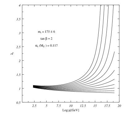
Figure 2: Focusing of the Yukawa couplings as $\lambda_{t}\to\lambda_{t}^{*}$.

The results displayed in Fig. 2 are perfectly consistent with having the ratio $m_{b}/m_{\tau}=1$, as SO(10) unification suggests, at scales of $O(M_{\rm Planck})$. An analysis similar to the one we did for Eq. (38) relates this ratio at a scale of $m_{t}$ to that at the unification scale $M_{X}\sim M_{\rm Planck}$:

$$\frac{m_{b}(m_{t})}{m_{\tau}(m_{t})}=\frac{m_{b}(M_{X})}{m_{\tau}(M_{X})}\left[\frac{\eta(M_{X})}{\hat{\eta}(M_{X})}\right]^{1/2}\left[\frac{\lambda_{t}(M_{X})}{\lambda_{t}(m_{t})}\right]^{-1/6}~{}.$$ (57)

Here $\hat{\eta}(\mu)$ is a quantity similar to $\eta(\mu)$, detailing the running of the coupling constants in the quark to lepton mass ratio:

$$\hat{\eta}(\mu)=\Pi_{i}\left(\frac{\alpha_{i}(m_{t})}{\alpha_{i}(\mu)}\right)^{\hat{c}_{i}/b_{i}}$$ (58)

with the coefficients $\hat{c}_{i}=\left(-\frac{4}{3}~{},~{}~{}0~{},~{}~{}\frac{16}{3}\right)$ for the MSSM. The ratio $[\eta(M_{X})/\hat{\eta}(M_{X})]^{1/2}\simeq 1.68$ is above the experimental ratio $m_{b}(m_{t})/m_{\tau}(m_{t})=1.58\pm 0.08$, suggesting that $\lambda_{t}(M_{X})\gg\lambda_{t}(m_{t})$. That is, the top coupling is stronger at the GUT scale than at low energy, much as indicated in Fig. 2.

The upshot of this discussion is that the assumption that supersymmetric matter exists above the weak scale gives a consistent picture, with a large top Yukawa coupling at the Planck scale being driven by an infrared fixed point to a value $\lambda_{t}(m_{t})\sim 1$. This behavior obtains in two regimes of $\tan\beta$. Either $\tan\beta\sim O(1)$ and $\lambda_{t}$ is the dominant coupling. Or $\lambda_{b}\sim\lambda_{t}$ and $\tan\beta$ is large. The second possibility is natural in the SO(10) models discussed earlier where all quarks and leptons of one family are in the 16-dimensional representation. Furthermore, at least intuitively, having a large Yukawa coupling at the Planck scale fits in well with the ideas that families are generated either dynamically or through geometry in supersymmetric theories.

VII Concluding Remarks

In my opinion, one probably will not be able to unravels the mystery of flavor without some new experimental information. In particular, I believe that ascertaining whether or not low energy supersymmetry exists will have a profound impact on this question. The discovery of low energy supersymmetry would, of course, provide a tremendous boost for superstring theories. At the same time, it would also signal the death knell of the random dynamics ideas of Nielsen. These ideas, if one is to believe in them, require that there should be a real desert up to $M_{\rm Planck}$, with no physics beyond the Standard Model between the weak and the Planck scale.

If supersymmetry is found, perhaps it is sensible to imagine that some of the ideas discussed in the previous section are true. That is, that there is indeed a large Yukawa coupling of top at energies of $O(M_{\rm Planck})$, which results in the mass of the top being determined essentially by the infrared fixed point of the Yukawa evolution equations. Furthermore, it is easy to imagine then that the quark and lepton mass spectrum is a result of a combination of a broken family symmetry–which sets up the hierarchy among the masses–and of a GUT–which interrelates the quark and lepton mass tapestries.

Even in this very favorite circumstance, however, it will be difficult to get real evidence for the origin of flavor. Is it due to dynamics or to some primordial compactification? Perhaps the tell-tale sign will emerge from the discovery of some exotic states, besides the quarks and leptons and their superpartners. In fact, the most characteristic signals of models for flavor is the inevitable presence of exotic states. Recall the exotic $T_{2}$ and $T_{3}$ states in the $Sp(6)$ model, or the extra $10\oplus 1$ states in the 27 produced through a Calabi-Yau compactification. In this respect, I should note that certain exotic states seem to be quite generic. In particular, the presence of extra $(3,1)_{-1/3}$ states is very natural.

On a more pedestrian level, our undestanding of flavor and mass will be aided by a continuous experimental (and theoretical) refinement of the values for the quark and lepton masses and mixing parameters. Precise values for these parameters are crucial if one wants to sort out alternative tapestries, signalling different origins for flavor. Eventually, it is going to be important to know that $V_{cb}=0.038$ rather than 0.040!

Acknowledgements

I am grateful to Ikaros Bigi and Luigi Moroni for their hospitality at the Varenna School. A condensed version of these lectures was presented in Chicago, Illinois, at the Symposium “20 Years of Beauty Physics”, while a more popular version was given as the first Abdus Salam Memorial Lecture in Islamabad, Pakistan. I thank Dan Kaplan and Ahmed Ali, respectively, for their kind invitations. This work is supported in part by the Department of Energy under Grant # DE-FOO3-91ER40662, Task C.

References

- (1) S. L. Adler, Phys. Rev. 177, 2426 (1969); J. Bell and R. Jackiw, Nuovo Cimento 51A, 47 (1969); W. A. Bardeen, Phys. Rev. 184, 1848 (1969).
- (2) S. Glashow and S. Weinberg, Phys. Rev. D15, 1958 (1977).
- (3) A shorter version of these lectures was presented at the symposium Twenty Years of Bottom Physics, Chicago, Illinois, July 1997, and will be published in the proceedings of this symposium.
- (4) D. B. Kaplan, F. Lepeintre and M. Schmaltz, hep-ph 9705411.
- (5) P. Cho and P. Kraus, Phys. Rev. D54, 7640 (1996); C. Czaki, W. Skiba, and M. Schmaltz, Nucl. Phys. B487, 128 (1997).
- (6) C. D. Froggatt and H. B. Nielsen, Nucl. Phys. B147, 727 (1979).
- (7) These ideas are discussed in considerable detail in the monograph Origin of Symmetries by C. D. Froggatt and H. B. Nielsen (World Scientific, Singapore, 1991).
- (8) H. B. Nielsen and N. Brene, Nucl. Phys. B236, 167 (1984); see also, Proceedings of the XVIII International Ahrenshoop Symposium (Akademie der Wissenschaften der DDR, Berlin-Zeuthen, 1985).
- (9) D. L. Bennett, H. B. Nielsen, and I. Picek, Phys. Lett. 208B, 275 (1988).
- (10) Th. Kaluza, Sitzungber Preuss. Akad. Wiss Berlin, Math. Phys. K1, 966 (1921); O. Klein, Nature 118, 516 (1926).
- (11) M. Green, J. Schwarz, and E. Witten Superstring Theory, Vols. 1 & 2 (Cambridge University Press, Cambridge, U.K. 1987).
- (12) C. Wetterich, Nucl. Phys. B223, 109 (1983).
- (13) E. Witten, in Proceedings of the 1983 Shelter Island Conference II (MIT Press, Cambridge, Mass., 1984).
- (14) A. Candelas, G. Horowitz, A. Strominger, and E. Witten, Nucl. Phys. B258, 46 (1985).
- (15) D. Gross, J. Harvey, E. Martinec, and R. Rohm, Nucl. Phys. B255, 257 (1985); B267, 75 (1986).
- (16) See. for example, B. R. Greene, K. H. Kirklin, P. J. Miron, and G. G. Ross, Nucl. Phys. B278, 667 (1986); B292, 606 (1987).
- (17) S. Weinberg, Transaction of the New York Academy of Sciences, Series II, 38, 185 (1977).
- (18) H. Fritzsch, Phys. Lett. 70B, 436 (1977).
- (19) S. Weinberg, Phys. Rev. D13, 974 (1976); L. Susskind, Phys. Rev. D20, 2619 (1979).
- (20) S. Dimopoulos and J. Ellis, Nucl. Phys. B182, 505 (1981).
- (21) B. Holdom, Phys. Rev. D24, 1441 (1981); Y. Yamamoto, M. Bando, and K. Matsumoto, Phys. Rev. Lett. 56, 1335; (1986); T. Akiba and T. Yanagida, Phys. Lett. 169B, 432 (1986); T. Appelquist, D. Karabali and L. Wijewardhana, Phys. Rev. Lett. 57, 982 (1986).
- (22) See, for example, B. Holdom, Phys. Lett. B246, 169 (1990); see also B. Holdom in Dynamical Symmetry Breaking, ed. K. Yamawaki (World Scientific, Singapore, 1992).
- (23) L. Ibañez and G. G. Ross, Phys. Lett. B332, 100 (1994).
- (24) See, for example, Y. Nir and N. Seiberg, Phys. Lett. B309, 337 (1993); M. Leurer, Y. Nir, and N. Seiberg, Nucl. Phys. B420, 468 (1994).
- (25) G. Anderson, S. Dimopoulos, L. J. Hall, S. Raby and G. Starkman, Phys. Rev. D49, 3660 (1974).
- (26) H. Georgi and C. Jarlskog, Phys. Lett. B86, 297 (1979).
- (27) T. Blazek, M. Carena, S. Raby and C. E. M. Wagner, hep-ph/9611217, Phys. Rev. (to be published).
- (28) V. Lucas and S. Raby, Phys. Rev. D55, 6986 (1997).
- (29) Particle Data Group, R. M. Barnett et al., Phys. Rev. D54, 1 (1995).
- (30) M. Olechowski and S. Pokorski, Phys. Lett. B257, 388 (1991).
- (31) L. Landau in Niels Bohr and the Development of Physics, ed. W. Pauli (McGraw Hill, New York,1955).
- (32) B. Schrempp and M. Wimmer, Progr. in Part. and Nucl. Phys. 37, 1 (1996).