We investigate numerical solution of the Dokshitzer-Gribov-Lipatov-Altarelli-Parisi (DGLAP) $Q^{2}$ evolution equation for the transversity distribution $\Delta_{{}_{T}}q$ or the structure function $h_{1}$. The leading-order (LO) and next-to-leading-order (NLO) evolution equations are studied. The renormalization scheme is $MS$ or $\overline{MS}$ in the NLO case. Dividing the variables $x$ and $Q^{2}$ into small steps, we solve the integrodifferential equation by the Euler method in the variable $Q^{2}$ and by the Simpson method in the variable $x$. Numerical results indicate that accuracy is better than 1% in the region $10^{-5}<x<0.8$ if more than fifty $Q^{2}$ steps and more than five hundred $x$ steps are taken. We provide a FORTRAN program for the Q² evolution and devolution of the transversity distribution $\Delta_{{}_{T}}q$ or $h_{1}$. Using the program, we show the LO and NLO evolution results of the valence-quark distribution $\Delta_{{}_{T}}u_{v}+\Delta_{{}_{T}}d_{v}$, the singlet distribution $\sum_{i}(\Delta_{{}_{T}}q_{i}+\Delta_{{}_{T}}\bar{q}_{i})$, and the flavor asymmetric distribution $\Delta_{{}_{T}}\bar{u}-\Delta_{{}_{T}}\bar{d}$. They are also compared with the longitudinal evolution results.

 

* Email: 96sm18@edu.cc.saga-u.ac.jp, kumanos@cc.saga-u.ac.jp, and

96td25@edu.cc.saga-u.ac.jp. Information on their research is available

at http://www.cc.saga-u.ac.jp/saga-u/riko/physics/quantum1/structure.html.

submitted for publication

Program Summary

Title of program: H1EVOL

Computer: AlphaServer 2100 4/200 (SUN-IPX); Installation: The Research Center for Nuclear Physics in Osaka (Saga University Computer Center)

Operating system: OpenVMS V6.1 (SunOS 4.1.3)

Programming language used: FORTRAN 77

Peripherals used: Laser printer

No. of lines in distributed program: 1203

Keywords: Polarized parton distribution, transversity distribution, chiral-odd structure function, Q² evolution, numerical solution.

Nature of physical problem

This program solves the DGLAP $Q^{2}$ evolution equation with or without next-to-leading-order (NLO) $\alpha_{s}$ effects for a transversely polarized parton distribution, so called transversity distribution $\Delta_{{}_{T}}q$ or chiral-odd structure function $h_{1}$.

Method of solution

The DGLAP integrodifferential equation is solved by dividing the variables $x$ and $Q^{2}$ into very small steps. The integrodifferential equation is solved step by step by the Euler method (“brute-force” method) in the variable $Q^{2}$ and by the Simpson method in the variable $x$.

Restrictions of the program

This program is used for calculating the $Q^{2}$ evolution of various transversity distributions $\Delta_{{}_{T}}q$ ($h_{1}$). The $Q^{2}$ evolution equation is the DGLAP equation. The double precision arithmetic is used. The minimal subtraction ($MS$) or the modified minimal subtraction ($\overline{MS}$) scheme is used in the NLO evolution. The NLO evolution is identical in both schemes. A user provides the initial distribution as a subroutine or as a data file. Examples are explained in Section 4. Then, the user inputs seventeen parameters in Section 4.

Typical running time

Approximately forty seconds on AlphaServer 2100 4/200 and two and a half minutes on SUN-IPX.

LONG WRITE-UP

1 Introduction

The European Muon Collaboration (EMC) shed light on the proton spin structure by measuring the longitudinally polarized structure function $g_{1}$. Its conclusion seemed startling: almost none of the proton spin is carried by quarks. Since then, many investigations have been done for understanding the internal spin structure of the proton. However, we should wait for refined experiments in order to determine each parton polarization, in particular polarized sea-quark and gluon distributions [1].

In addition to the abovementioned studies on the longitudinal polarization, it is interesting to test the spin structure in the transverse polarization. There exists a leading-twist structure function which will be measured in the transversely polarized Drell-Yan processes [2, 3, 4]. It is now named as the $h_{1}$ structure function [3], which measures the transversity distribution, $\Delta_{{}_{T}}q$ or often denoted as $\delta q$. It has a chiral-odd property so that it cannot be found in inclusive deep inelastic electron scattering. The $h_{1}$ structure function is expected to be measured in the Relativistic Heavy Ion Collider (RHIC) Spin project [5] at Brookhaven National Laboratory. The experimental results will provide us a good opportunity to understand unexplored transverse spin physics at high energies. Furthermore, semi-inclusive electron deep inelastic scattering could also reveal the $h_{1}$ although there is a complication of unknown fragmentation functions [6]. With these experimental possibilities in mind, theoretical physicists should investigate detailed properties of $h_{1}$ [7] as far as they can before the completion of the RHIC facility.

There are, in general, two variables in the structure functions: $Q^{2}$ and the momentum fraction $x$. In the transversity distribution measured by the Drell-Yan, $Q^{2}$ is the dimuon-mass square: $Q^{2}=m_{\mu\mu}^{2}$. The $x$ distribution is associated with nonperturbative physics, which can be handled only in certain quark models at this stage because there is no experimental information on $h_{1}$. The lattice QCD calculation is not still very reliable as far as the $x$ distribution is concerned [8]. On the other hand, the $Q^{2}$ dependence can be predicted in perturbative Quantum Chromodynamics (QCD) unless $Q^{2}$ is small. This scaling violation is described by the Dokshitzer-Gribov-Lipatov-Altarelli-Parisi (DGLAP) equation [9], which is an integrodifferential equation. The leading-order (LO) DGLAP equation for $h_{1}$ was derived in Ref. [10] and its numerical analysis is discussed in Ref. [11]. In addition, the next-to-leading order (NLO) analysis for its anomalous dimensions and splitting function was completed recently for the transversity distribution $\Delta_{{}_{T}}q$. The NLO evolution of $\Delta_{{}_{T}}q$ was studied in the Feynman gauge [12] and in the light-cone gauge [13]. It was also investigated in the Feynman gauge in a subsequent paper [14, 15]. The results made it possible to investigate the details of NLO evolution effects in the structure function $h_{1}$ [16, 17, 18]. In particular, the NLO analysis is usually used in the unpolarized structure functions and in the longitudinally polarized structure function $g_{1}$. The NLO studies can be extended now to the $h_{1}$ case. In this paper, we report our studies on the numerical solution.

Our group has been investigating the numerical solution in the unpolarized structure functions and also in the polarized structure function $g_{1}$. So far, we employed the Laguerre-polynomial [19] and the brute-force [20] methods. Other methods with the Mellin transformation are, for example, discussed in Ref. [21]. The variables $Q^{2}$ and $x$ are divided into small steps, then the integrodifferential equation is solved step by step in Ref. [20]. Because the scaling violation is a small logarithmic effect, the integration over $Q^{2}$ is accurately done with a small number of steps. In this paper, we change the brute-force integration over $x$ to the Simpson method with expectation of better accuracy. The transversity evolution is rather simple in the sense that the gluon does not couple to the distribution $\Delta_{{}_{T}}q$ because of the chiral-odd nature. Therefore, the evolution equation is a single integrodifferential equation without mixing with the gluon distribution. It is the same form as the nonsinglet evolution equation. This fact simplifies our numerical analysis. The transversity evolution is completed by solving only the “nonsinglet-type” evolution equation.

The purpose of our study is to provide a useful $Q^{2}$ evolution program for the distribution $\Delta_{{}_{T}}q$ (or $h_{1}$). It should be very useful for theoretical and experimental researchers who are involved in the RHIC-Spin type project or in semi-inclusive lepton scattering one for finding $h_{1}$. We explain the details of our studies in the following. In Section 2, the transversity DGLAP $Q^{2}$ evolution equation is explained. Then, our numerical-solution method is described in Section 3. Input parameters and input distributions are discussed in Section 4, and subroutines in the program are explained in Section 5. Numerical results and their comparison with longitudinally polarized distributions are discussed in Section 6. Summary is given in Section 7. Explicit forms of splitting functions are listed in Appendices.

2 $\bf Q^{2}$ evolution equation for the transversity
distribution $\bf\Delta_{{}_{T}}q$

The transversity distribution $\Delta_{{}_{T}}q_{i}$, which is equivalently denoted as $h_{1}^{i}$ or $\delta q_{i}$, with the quark flavor $i$ can be measured, for example, in the double transverse-spin asymmetry $A_{TT}$ in the Drell-Yan process [2, 3, 4]:

$$A_{TT}=\frac{\sin^{2}\theta\,\cos 2\phi}{1+\cos^{2}\theta}\frac{\sum_{i}e_{i}^{2}\,\Delta_{{}_{T}}q_{i}(x_{1})\,\Delta_{{}_{T}}\bar{q}_{i}(x_{2})}{\sum_{i}e_{i}^{2}\,q_{i}(x_{1})\,\bar{q}_{i}(x_{2})}\ .$$ (2.1)

The factor $a_{{}_{TT}}=\sin^{2}\theta\,\cos 2\phi/(1+\cos^{2}\theta)$ is the parton’s double asymmetry. The angles $\theta$ and $\phi$ are the polar and azimuthal angles of the lepton momentum with respect to the beam and proton polarization directions respectively. According to the above equation, the distribution combination $\Delta_{{}_{T}}q_{i}\,\Delta_{{}_{T}}\bar{q}_{i}$ weighted by the charge square can be measured with information on the unpolarized distributions $q_{i}$ and $\bar{q}_{i}$. The spin asymmetry $A_{TT}$ will be measured in the RHIC-Spin project [5], and the transversity distributions could be obtained by Eq. (2.1).

The distribution $\Delta_{{}_{T}}q$ is interpreted in a parton model: it is the probability to find a quark with spin polarized along the transverse spin of a polarized proton minus the probability to find it polarized oppositely ($\Delta_{{}_{T}}q=q_{\uparrow}-q_{\downarrow}$). The LO evolution equation for $\Delta_{{}_{T}}q$ was derived in Ref. [10], and the NLO evolution of $\Delta_{{}_{T}}q$ was recently obtained in Refs. [12, 13, 14]. Because of the chiral-odd nature of the transversity distribution $\Delta_{{}_{T}}q$ or the structure function $h_{1}$, the gluon does not participate in the evolution equation. Therefore, the DGLAP equation is a single integrodifferential equation:

$$\frac{\partial}{\partial\ln Q^{2}}\,\Delta_{{}_{T}}q^{\pm}(x,Q^{2})\,=\frac{\alpha_{s}(Q^{2})}{2\pi}\,\Delta_{{}_{T}}P_{q^{\pm}}(x)\otimes\Delta_{{}_{T}}q^{\pm}(x,Q^{2})\ ,$$ (2.2)

where $\Delta_{{}_{T}}P_{q^{\pm}}$ is the splitting function for the transversity distribution. The convolution $\otimes$ in Eq. (2.2) is defined by

$$f(x)\otimes g(x)=\int^{1}_{x}\frac{dz}{z}f\left(\frac{x}{z}\right)g(z)\ .$$ (2.3)

The notation $q^{\pm}$ in the splitting function indicates the $\Delta_{{}_{T}}q^{+}=\Delta_{{}_{T}}q+\Delta_{{}_{T}}\bar{q}$ or $\Delta_{{}_{T}}q^{-}=\Delta_{{}_{T}}q-\Delta_{{}_{T}}\bar{q}$ distribution type. The $\alpha_{s}(Q^{2})$ is the running coupling constant. Both LO and NLO evolution calculations can be handled by Eq. (2.2); however, there are differences between the LO and NLO splitting functions and also between the coupling constants. The LO and NLO expressions for $\Delta_{{}_{T}}P_{q^{\pm}}$ [13] and $\alpha_{s}$ are listed in Appendix A. In the following numerical analysis, we use the variable $t$ which is defined by

$$t\equiv\ln Q^{2}$$ (2.4)

instead of $Q^{2}$. Furthermore, the parton distribution and the splitting function multiplied by $x$,

$$\widetilde{f}(x)=xf(x)\ ,$$ (2.5)

are used throughout this paper because they satisfy the same integrodifferential equation. Then, Eq. (2.2) becomes

$$\frac{\partial}{\partial t}\,\Delta_{{}_{T}}\widetilde{q}^{\,\,\pm}(x,t)=\frac{\alpha_{s}(t)}{2\pi}\,\Delta_{{}_{T}}\widetilde{P}_{q^{\pm}}(x)\otimes\Delta_{{}_{T}}\widetilde{q}^{\,\,\pm}(x,t)\ .$$ (2.6)

3 Simpson method

There are various numerical methods for solving the DGLAP equations [21]. We have investigated two methods, the Laguerre-polynomial [19] and the brute-force [20] methods. The splitting functions and parton distributions are expanded by the Laguerre polynomials in the first method. Even though the Laguerre method has an advantage of computing time, it may not be very accurate in the spin-independent nonsinglet case at small $x$. In the brute-force method, the variables $t$ and $x$ are divided into small steps, then the integral is calculated in the simplest manner. This method is accurate if a large number of steps is taken. However, it inevitably takes much computing time. In order to resolve these problems, the Simpson method [22] is employed in the $z$ integration of Eq. (2.3). Here, we report its numerical analysis.

In the following numerical solution, the brute-force method is still used in the variable $t$ and the Simpson method is introduced in calculating the $z$ integration. The brute-force method for solving a differential equation is often called Euler method [22], so that we use this terminology in this paper. The variables $t$ and $z$ are divided into $N_{t}$ and $N_{z}$ steps, then differentiation and integration are defined by

$$\frac{df(t)}{dt}= \,\frac{f(t_{j+1})-f(t_{j})}{\delta t}\ ,$$ (3.1)

$$\int g(z)\ dz= \sum_{k=2}^{N_{z}}\,\frac{\delta z}{3}\,[\,g(z_{k-1})+4g(z_{k})+g(z_{k+1})\,]\ ,$$

$$where\ \ k=2,\,4,\,\cdot\cdot\cdot,\,N_{z}\ \ \ \ \ .$$ (3.2)

The $k$ summation is taken over the even numbers from 2 to $N_{z}$, so that $N_{z}$ has to be an even number.

With these replacements, the evolution equation can be solved rather easily. Equation (2.6) is written in the following form:

$$\Delta_{{}_{T}}\widetilde{q}^{\,\,\pm}(x_{m},t_{j+1})= \,\Delta_{{}_{T}}\widetilde{q}^{\,\,\pm}(x_{m},t_{j})+\delta t\,\frac{\alpha_{s}(t_{j})}{2\pi}\,\sum_{k=2m}^{N_{z}}\frac{\delta z}{3z_{k}}\,F(z_{k},x_{m},t_{j})$$

$$k=2m,\,2m+2,\,\cdot\cdot\cdot,\,N_{z}\ \ \ \ \ \ ,$$ (3.3)

where the variable $x$ is divided into $N_{x}=N_{z}/2$ steps. The function $F$ is defined by the following:

$$F(z_{k},x_{m},t_{j})=\, \Delta_{{}_{T}}\widetilde{P}_{q^{\pm}}(z_{k-1})\,\Delta_{{}_{T}}\widetilde{q}^{\,\,\pm}\left(\frac{x_{m}}{z_{k-1}},t_{j}\right)+4\ \Delta_{{}_{T}}\widetilde{P}_{q^{\pm}}(z_{k})\,\Delta_{{}_{T}}\widetilde{q}^{\,\,\pm}\left(\frac{x_{m}}{z_{k}},t_{j}\right)$$

$$\ +\Delta_{{}_{T}}\widetilde{P}_{q^{\pm}}(z_{k+1})\,\Delta_{{}_{T}}\widetilde{q}^{\,\,\pm}\left(\frac{x_{m}}{z_{k+1}},t_{j}\right)\ .$$ (3.4)

First, the evolution from $t_{1}=\ln Q_{0}^{2}$ to $t_{2}=t_{1}+\delta t$ is calculated in the above equation by providing the initial distribution $\Delta_{{}_{T}}\widetilde{q}^{\,\,\pm}(x_{m}/z_{k},t_{j=1})$. Repeating this step $N_{t}-1$ times, we obtain the final distribution at $t=t_{N_{t}+1}$. However, the small $x$ region is often important practically. If the accurate results are required in the small $x$ region, $x$ and $z$ should be replaced by $\log_{10}x$ and $\log_{10}z$. Then, the evolution equation Eq. (2.6) is replaced by

$$\frac{\partial}{\partial t}\Delta_{{}_{T}}\widetilde{q}^{\,\,\pm}(\log_{10}x,t)=\ln 10\ \frac{\alpha_{s}(t)}{2\pi}\int_{\log_{10}x}^{0}\!\!\!\!\!\!\!\!d(\log_{10}z)\Delta_{{}_{T}}\widetilde{P}_{q^{\pm}}(\log_{10}z)\Delta_{{}_{T}}\widetilde{q}^{\,\,\pm}\left(\log_{10}\frac{x}{z},t\right)\,.$$ (3.5)

In order to apply the Simpson method to this equation, $\log_{10}x$ and $\log_{10}z$ are divided into $N_{x}$ and $N_{z}$ steps. Our FORTRAN code supports both the linear-step and the logarithmic-step cases, and the details are explained in the following sections.

4 Description of input parameters and initial
distribution

For running the FORTRAN-77 program H1EVOL, a user should supply seventeen input parameters from the file #10. In addition, an input distribution(s) should be given in a function subroutine(s) in the end of the FORTRAN program or in an input data file(s). The $i$-th initial distribution is written in the output file #30+$i$ (#31 – #38). Evolution results for the distribution-$i$ are written in the output file #20+$i$ (#21 – #28). The maximum number of the input distributions is eight. We explain the input parameters and the initial distributions in the following.

4.1 Input parameters

There are following seventeen parameters.

IREP	1	finish the program after this evolution
	2	proceed to the next evolution with new input parameters
IOUT	1	write $x$ and $x\Delta_{{}_{T}}q(x)$ at fixed $Q^{2}$ (=Q2) in the file(s) #21 – #28
	2	write $Q^{2}$ and $x\Delta_{{}_{T}}q(Q^{2})$ at fixed $x$ (=XX) in the file(s) #21 – #28
IREAD	1	give initial distribution(s) in function subroutine(s)
	2	give initial distribution(s) from the file(s) #11 – #18
INDIST	1	do not write initial distribution(s)
	2	write initial distribution(s) in the file(s) #31 – #38
	3	write initial distribution(s) in the file(s) #31 – #38
		without calculating evolution
IORDER	1	leading order (LO) in $\alpha_{s}$
	2	next-to-leading order (NLO)
IMORP	1	$x\Delta_{{}_{T}}q_{i}-x\Delta_{{}_{T}}\bar{q}_{i}$ type distribution
	2	$x\Delta_{{}_{T}}q_{i}+x\Delta_{{}_{T}}\bar{q}_{i}$ type distribution
ILOG	1	linear-$x$ and linear-$z$ steps are taken in calculating the evolution
		and in writing the $x$-dependent output.
	2	logarithmic-$x$ and logarithmic-$z$ steps
		(We recommend to use ILOG=2 in a general case.)

Q02	initial $Q^{2}$ ($\equiv Q_{0}^{2}$ in GeV2 ) at which an initial distribution is supplied
Q2	$Q^{2}$ to which the distribution is evolved ($Q^{2}\neq Q_{0}^{2}$, $Q^{2}>Q_{0}^{2}$ or $Q^{2}<Q_{0}^{2}$)
DLAM	QCD scale parameter $\Lambda_{QCD}$ in GeV
NF	number of quark flavors $N_{f}$
XX	$x$ at which $Q^{2}$ dependent distributions are written (IOUT=2 case)
NX	number of $x$ steps $N_{x}$ (NX $\leq$ 3000)
NT	number of $t$ steps $N_{t}$ (NT $\leq$ 3000)
NSTEP	number of $x$ steps or $t$ steps for writing output distribution(s)
XMIN	minimum of $x$, $x_{min}$ (0 $<$ XMIN $<$ XX)
NFI	number of distributions which are evolved simultaneously (NFI $\leq$ 8)

Numerical values of the parameters should be supplied in the file #10, then these are read in the program through the subroutine GETPA1. It should be noted that the first four lines of the file #10 are comments. Therefore, the parameters are given from the fifth line as shown in the following example. There are irrelevant parameters in some cases:

$$IOUT=1 case \cdot\cdot\cdot\ \ XX$$

$$INDIST=3 case \cdot\cdot\cdot\ \ IORDER,IMORP,Q2,DLAM,NF,XX,NT$$

$$IORDER=1 case \cdot\cdot\cdot\ \ IMORP\ \ .$$

Although they are not used in running the evolution part, their numerical values should be supplied in the file #10 within the allowed ranges.

The meaning of IREAD is explained in Section 4.2. The parameter IMORP indicates a plus or minus type distribution $\sum_{i}a_{i}x(\Delta_{{}_{T}}q_{i}\pm\Delta_{{}_{T}}\bar{q}_{i})$, where $a_{i}$ are some constants. In the NFI $\geq$ 2 case, distributions with the same $\pm$ type can be evolved at the same time. The maximum number of the distributions is set up as eight in the program. For example, if one would like to evolve two $\Delta_{{}_{T}}q^{+}$ type initial distributions at $Q^{2}$=4.0 GeV² to the distributions at $Q^{2}$=200.0 GeV² by the NLO DGLAP equation with $N_{f}$=4 and $\Lambda$=0.231 GeV, the input parameters could be IREP=1, IOUT=1, IREAD=1, INDIST=1, IORDER=2, IMORP=2, ILOG=2, Q02=4.0, Q2=200.0, DLAM=0.231, NF=4, XX=0.1, NX=500, NT=50, NSTEP=50, XMIN=0.0001, and NFI=2. In this case, the input file #10 is:

———————————————————————

IREP,IOUT,IREAD,INDIST,IORDER,IMORP,ILOG

Q02,Q2,DLAM,NF,XX,NX,NT,NSTEP,XMIN,NFI

———————————————————————

1, 1, 1, 1, 2, 2, 2

4.0, 200.0, 0.231, 4, 0.1, 500, 50, 50, 0.0001, 2

The first four lines are comments. The parameter values from IREP to ILOG should be written in the fifth line and the remaining ones in the next line. If one would like to repeat the evolution, for example if the LO evolution is also needed, the input file is the following:

———————————————————————

IREP,IOUT,IREAD,INDIST,IORDER,IMORP,ILOG

Q02,Q2,DLAM,NF,XX,NX,NT,NSTEP,XMIN,NFI

———————————————————————

2, 1, 1, 1, 2, 2, 2

4.0, 200.0, 0.231, 4, 0.1, 500, 50, 50, 0.0001, 2

1, 1, 1, 1, 1, 2, 2

4.0, 200.0, 0.231, 4, 0.1, 500, 50, 50, 0.0001, 2

In the same way, one can repeat the evolution further by choosing IREP=2. The evolved results are written continuously in the same output file(s).

4.2 Initial distributions supplied by function subroutines
(IREAD=1)

If IREAD=1 is chosen, an input distribution(s) at $Q_{0}^{2}$ should be supplied in the end of the FORTRAN program H1EVOL as a function subroutine(s) H1IN1(X) – H1IN8(X). For example, three distributions (e.g. $x\Delta_{{}_{T}}u^{+}$, $x\Delta_{{}_{T}}d^{+}$, and $x\Delta_{{}_{T}}s^{+}$) can be evolved at the same time in the NFI=3 case. These initial distributions should be supplied in the function subroutines H1IN1(X), H1IN2(X), and H1IN3(X). The remaining functions H1IN4(X) – H1IN8(X) may be set to zero. The evolution results for the initial distribution-i, which is given by the function H1INi(X) (i=1, 2, $\cdot\cdot\cdot$, NFI), are written in the output file #20+i. If INDIST=2 or 3 is chosen, the initial distribution(s) is written in the file #30+i.

To be exact, there is no information on the input transversity distribution because experimental data do not exist. We discuss this point in Section 6.1. In our program, the Gehrmann-Stirling (GS) type-A [23] singlet distribution $x\Delta_{{}_{T}}q_{{}_{S}}\equiv\sum_{i}^{N_{f}}(x\Delta_{{}_{T}}q_{i}+x\Delta_{{}_{T}}\bar{q}_{i})$ is given in the function H1IN1(X), and the distribution $[(x\Delta_{{}_{T}}u+x\Delta_{{}_{T}}\bar{u})-(x\Delta_{{}_{T}}d+x\Delta_{{}_{T}}\bar{d})]/2$ is given in H1IN2(X). Additionally, the valence-quark distribution $x\Delta_{{}_{T}}u_{{}_{V}}+x\Delta_{{}_{T}}d_{{}_{V}}$ is given in the function H1IN1(X) and the distribution $[(x\Delta_{{}_{T}}u-x\Delta_{{}_{T}}\bar{u})-(x\Delta_{{}_{T}}d-x\Delta_{{}_{T}}\bar{d})]/2$ is given in H1IN2(X) as comments.

4.3 Initial distributions supplied by data files
(IREAD=2)

If IREAD=2 is chosen, an input distribution(s) at $Q_{0}^{2}$ should be supplied in a separate data file(s) # 11 – #18 as shown in the following. We give the singlet distribution as an example.

0.000100	0.001721
0.000110	0.001612
0.000120	0.001485
0.000132	0.001339
0.000145	0.001172
…	…
…	…
…	…
1.000000	0.000000

The first column is the $x$ values and the second one is the corresponding distribution values. The data should be sorted from the smallest $x$ to larger ones, and the data at $x\leq x_{min}$ and at $x$=1.0 must be supplied. The last line number should be smaller than three thousand. The evolution results for the initial distribution in the file #10+i (i=1, 2, $\cdot\cdot\cdot$, NFI) are written in the file #20+i. If INDIST=2 or 3 is chosen, the initial distribution(s) at NSTEP+1 points is written in the file(s) #30+i.

5 Description of the program H1EVOL

5.1 Main program H1EVOL

The seventeen input parameters are read by calling the subroutine GETPA1 and these parameters are checked by the subroutine ERR1. If there is an error, the program writes the error message in the output file #6 and stops. Color constants and other necessary constants are calculated in the subroutine GETPA2. Then, $t$, $x$, $z$, and the splitting function are evaluated at each step point by the subroutines GETT, GETX, GETZ, and GETP respectively. If IOUT=2 is chosen, the XMIN is replaced by XX and $x$ values in the array X(I) are shifted in the subroutine GETMIN so as to have X(1)=XX, $\cdot\cdot\cdot$, X(NX+1)=1.0. The initial distribution(s) is calculated in the subroutine GETINI or is read from the data file(s) by the subroutine REDINI, then it is stored in the array H1(IN,I). Here, the argument IN is the distribution number from 1 to NFI. The initial distribution(s) is written in the file(s) #30+IN by the subroutine OUTXD if INDIST$\neq$1.

Since all the necessary values are ready in the above procedures, we start the evolution calculation. First, the initial distribution(s) is stored in the array WH1(IN,I) and $\alpha_{s}$ at $t_{1}$ is calculated by the subroutine GETALP. The evolved distribution(s) at $t_{2}=t_{1}+\delta t$ is calculated by the subroutines GETINT and GETH1, and the results are stored in H1(IN,I). If IOUT=2, the result(s) at $x$ = XX is stored in the array H1Q2(IN,I). Next, the evolution results are stored in WH1(IN,I) and $\alpha_{s}$ at $t_{2}$ is evaluated. Then, the evolution from $t_{2}$ to $t_{3}=t_{2}+\delta t$ is calculated in the same way. Repeating this step, we obtain the final distribution(s) at $t=t_{N_{t}+1}$. The calculated values are interpolated either in $t$ or in $x$ depending on IOUT by using the subroutine SPLINE and the function SEVAL. The final results at NSTEP+1 points are written in the output file(s) #10+IN by the subroutines OUTXD or OUTQ2D.

5.2 Subroutines GETPA1(IREP,IEORD,IERR), GETPA2,
and ERR1(IREP,IERR)

The subroutine GETPA1 reads the seventeen input parameters from the input file #10. These parameters are checked whether they are within the valid ranges by the subroutine ERR1. If there is an error, IERR=1 is returned from the subroutine ERR1 and the program stops with warning notification in the file #6. The subroutine GETPA2 calculates necessary color constants, $\pi$, $\beta_{0}$, and $\beta_{1}$.

5.3 Subroutines GETT(Q02,Q2,NT,T,DT)
and GETX(XMIN,XMAX,NX,ILOG,X,DX)

These subroutines evaluate the values of $t=\ln Q^{2}$ and $x$ at $N_{t}+1$ and $N_{x}+1$ points, and they are stored in the arrays T(I) with I=1, 2, $\cdot\cdot\cdot$, $N_{t}+1$ and X(I) with I=1, 2, $\cdot\cdot\cdot$, $N_{x}+1$. In the subroutine GETX, either the linear-$x$ (ILOG=1 case) or logarithmic-$x$ (ILOG=2 case) step is chosen. These subroutines also return the value of $\delta t=[t(Q^{2})-t(Q_{0}^{2})]/N_{t}=DT$ and $\delta x=DX$, where $\delta x$ is defined by $\delta x=(1-x_{min})/N_{x}$ in the ILOG=1 case or $\delta x=(0-\log_{10}x_{min})/N_{x}$ in the ILOG=2 case.

5.4 Subroutine GETMIN(XX,X,NX,XMIN)

In the IOUT=2 case, the subroutine GETMIN is called after getting X(I). This subroutine replaces the XMIN value by XX because the distribution information at $x<XX$ is not necessary in the evolution calculation. Then, the values in the array X(I) are shifted. For example, if XX is in the region X(M) $<$ XX $<$ X(M+1), X(1) is replaced by XX and X(2), X(3), $\cdot\cdot\cdot$, X(NX$-$M+2) are replaced by X(M+1), X(M+2), $\cdot\cdot\cdot$, X(NX+1). The number of steps $N_{x}$ is also replaced by $N_{x}-M+1$.

5.5 Subroutine GETZ(ILOG,X,NX,DX,Z,NZ,DZ)

The subroutine GETZ calculates the values of $z$ at $N_{z}+1$ $(N_{z}=2N_{x})$ points and stores these values into the array Z(K), K=1, 2, $\cdot\cdot\cdot$, $N_{z}+1$. The first one is given by $\rm Z(1)=X(1)$, and the second one Z(2) is calculated by ${\rm Z(2)}={\rm Z(1)}+[{\rm X(2)}-{\rm X(1)}]/2$ in ILOG=1 case or ${\rm Z(2)}={\rm Z(1)}+[\log_{10}{\rm X(2)}-\log_{10}{\rm X(1)}]/2$ in ILOG=2 case. The subsequent ones are given by Z(3)=X(2), Z(4)=Z(3)+$\delta x$/2, Z(5)=X(3), Z(6)=Z(5)+$\delta x$/2, $\cdot\cdot\cdot$ in the ILOG=1 case or by Z(3)=X(2), $\log_{10}$Z(4)=$\log_{10}$Z(3)+$\delta x$/2, Z(5)=X(3), $\log_{10}$Z(6)=$\log_{10}$Z(5)+$\delta x$/2, $\cdot\cdot\cdot$ in the ILOG=2 case.

5.6 Subroutine GETP(IORDER,SIGN)

The subroutine GETP calculates the LO and NLO splitting functions at the $N_{z}+1$ points and stores the calculated values in the arrays P0(K), P0PF(K), P1(K) and P1PF(K). The splitting functions are calculated by the functions PLO, P0PL, PNLO, and P1PL. Additionally, the extra factors associated with the ‘+’ function or $\delta$ function are also evaluated by calling the subroutines P0DL and P1DL.

5.7 Subroutines GETINI(NFI,H1) and REDINI(NFI,H1,IERR)

If IREAD=1 is chosen, the subroutine GETINI calculates the initial distribution(s) by calling the function(s) H1IN1(X) – H1IN8(X). The subroutine REDINI reads the initial distribution(s) from the input data file(s) and interpolates the distributions(s) by using SPLINE and SEVAL if IREAD=2.

5.8 Subroutine GETALP(T,IORDER,ALP2PI)

The subroutine GETALP calculates the $\alpha_{s}/2\pi$=ALP2PI at given $t$.

5.9 Subroutines GETINT(DINTEG), FUN(K,I,IN),
and SIMPS(FUN,I,IN,DZ)

The subroutine GETINT calculates the integral by calling the subroutine SIMPS. The SIMPS integrates the integrand FUN by using the Simpson method. The integral results in the array DINTEG are then returned. The factor IN is the input distribution number, IN=1, 2, $\cdot\cdot\cdot$, or NFI. The factors K and I represent the $z$ and $x$ positions, Z(K) and X(I).

5.10 Subroutine GETH1(DT1,DINTEG,H11)

The subroutine GETH1 calculates the distribution at $t=t_{j}$ from the one at $t=t_{j-1}$ with the integral obtained by GETINT. The evolution results are stored in H11(IN,I). The factor DT1 is the $t$ step.

5.11 Subroutines OUTXD(ILOG,H1,NFILE)
and OUTQ2D(Q2T,H1Q2)

These subroutines interpolate the final evolution results and write the distribution(s) at NSTEP+1 points in the output file(s). The OUTXD (OUTQ2D) writes the $x$ ($Q^{2}$) dependent results. The OUTXD is also used for writing the initial distribution(s) in the INDIST=2 or 3 case. The NFILE is the factor for writing either the initial distribution (NFILE=1) or the final one (NFILE=2).

5.12 Subroutine SPLINE(N,X,Y,B,C,D,IN)
and function SEVAL(N,XX,X,Y,B,C,D,IN)

The subroutine SPLINE calculates the coefficients, B(IN,I), C(IN,I), and D(IN,I) ($I=1,2,\cdot\cdot\cdot,N$) by the cubic Spline interpolation for the distribution type IN. The interpolated points Y(IN,I) at X(I) ($I=1,2,\cdot\cdot\cdot,N$) should be supplied. This interpolation program is taken from Ref. [24]. Using the obtained Spline coefficients, the function SEVAL calculates the value of Y at given XX.

5.13 Functions PLO(Z), P0PL(Z), PNLO(Z,SIGN),
and P1PL(Z)

The functions PLO and PNLO calculate the LO and NLO splitting functions. The functions P0PL and P1PL calculate the LO and NLO ‘+’ function parts in the splitting functions. If IMORP=1 (SIGN=$-$1.0), the PNLO calculates the $\Delta_{{}_{T}}q-\Delta_{{}_{T}}\bar{q}$ type splitting function, and it calculates the $\Delta_{{}_{T}}q+\Delta_{{}_{T}}\bar{q}$ type if IMORP=2 (SIGN=+1.0).

5.14 Subroutines P0DL(PLUS0,DEL0) and P1DL(PLUS1,DEL1)

The subroutines P0DL and P1DL calculate the extra factors which are related to the ‘+’ function [see the second term of Eq. (A.8)] and the $\delta$ function. These factors are taken out from the integral.

5.15 Functions S2(Z), SPENCE(X), and DGAUSS(EXTERN,A,B)

The function S2 calculates $S_{2}(x)$ which appears in the splitting function. The $S_{2}(x)$ is expressed in terms of the Spence function in Eq. (A.12). The Spence function is defined by the integral form in Eq. (A.13), and it is numerically calculated by the function DGAUSS in the Gauss-Legendre method with the integrand SPENCE.

5.16 Function GS(X,A,B,C,D,E,F)

This function calculates the GS type parton distribution with the parameters A, B, C, D, E, and F as $ABx^{C}(1-x)^{D}(1+Ex+F\sqrt{x})$.

5.17 Functions H1IN1(X), H1IN2(X), $\cdot\cdot\cdot$, and H1IN8(X)

These functions calculate the initial distributions. For example, three initial distributions should be provided in the NFI=3 case by H1IN1(X), H1IN2(X), and H1IN3(X), and the remaining functions should be set to zero.

6 Numerical analysis

6.1 Accuracy of $\bf Q^{2}$ evolution results

There are two parameters which determine the accuracy of our numerical results. They are the numbers of steps: $N_{x}$ and $N_{t}$. Another number of steps $N_{z}$ is fixed by the relation $N_{z}=2N_{x}$. In this subsection, we discuss how the evolution results depend on these parameters and how long it takes for calculating the evolution.

There is a practical problem in the transversity evolution in the sense that there is no input distribution. For example, the input parton distributions are obtained by fitting various experimental data in the unpolarized distribution studies. At this stage, there is no experimental information on the transversity distribution, so that the initial distribution could not be supplied. An item of good news is that the lattice QCD studies started producing a $x$ distribution [8] although it is still somewhat away from the very reliable one. Therefore, we may use the initial distribution calculated by a bag model [3], a nonrelativistic quark model [16, 25], or the Glück-Reya-Stratmann-Vogelsang distribution [26, 11] at very small $Q^{2}$. It is known that the transversity distribution and the corresponding longitudinally polarized one are almost the same at small $Q^{2}$ according to Ref. [3]. However, the applicability of perturbative QCD becomes dubious in the small $Q^{2}$ region. Therefore, instead of stepping into the nonperturbative region, we decided to use a longitudinally polarized distribution at larger $Q^{2}$ as the input transversity distribution. The Gehrmann-Stirling (GS) type-A distributions [23] are used throughout this paper. They are given at $Q^{2}$=4 GeV². We warn the reader that the assumption $\Delta q=\Delta_{{}_{T}}q$ would not be valid in the $Q^{2}$=4 GeV² region even though it would work at small $Q^{2}$ ($\sim\Lambda_{QCD}^{2}$). Future experimental data will clarify the difference between the two distributions.

We show the dependence on $N_{x}$ and $N_{t}$ by taking the singlet distribution. First, we fix the $x$-step number at $N_{x}$=1000, then the $t$-step number $N_{t}$ is varied as 10, 50, 200, and 1000. The input distribution is the GS-A singlet distribution at $Q^{2}$=4 GeV² [23]. Because there is little information on each antiquark distribution [27], flavor symmetric distributions are assumed for the antiquark distributions. Calculated evolution results for the distribution $x\Delta_{{}_{T}}q_{{}_{S}}\equiv x\sum_{i}^{N_{f}}(\Delta_{{}_{T}}q_{i}+\Delta_{{}_{T}}\bar{q}_{i})$ are shown in Fig. 1. We use $N_{f}=$4 and $\Lambda$=231 MeV in calculating the evolution. The GS-A singlet distribution is evolved to the one at $Q^{2}$=200 GeV² by our NLO program. The initial distribution is supplied at the end of the program as the subroutine H1IN1(X). The input parameters are IREP=1, IOUT=1, IREAD=1, INDIST=1, IORDER=2, IMORP=2, ILOG=2, Q02=4.0, Q2=200.0, DLAM=0.231, NF=4, XX=0.1, NX=1000, NT=10, 50, 200, or 1000, NSTEP=100, XMIN=0.0001, and NFI=1. There is almost no difference between the various results in Fig. 1 except for the $N_{t}$=10 case. It means that merely fifty steps are enough for the getting the accurate evolution. The small number of steps is enough because the scaling violation is a small logarithmic effect.

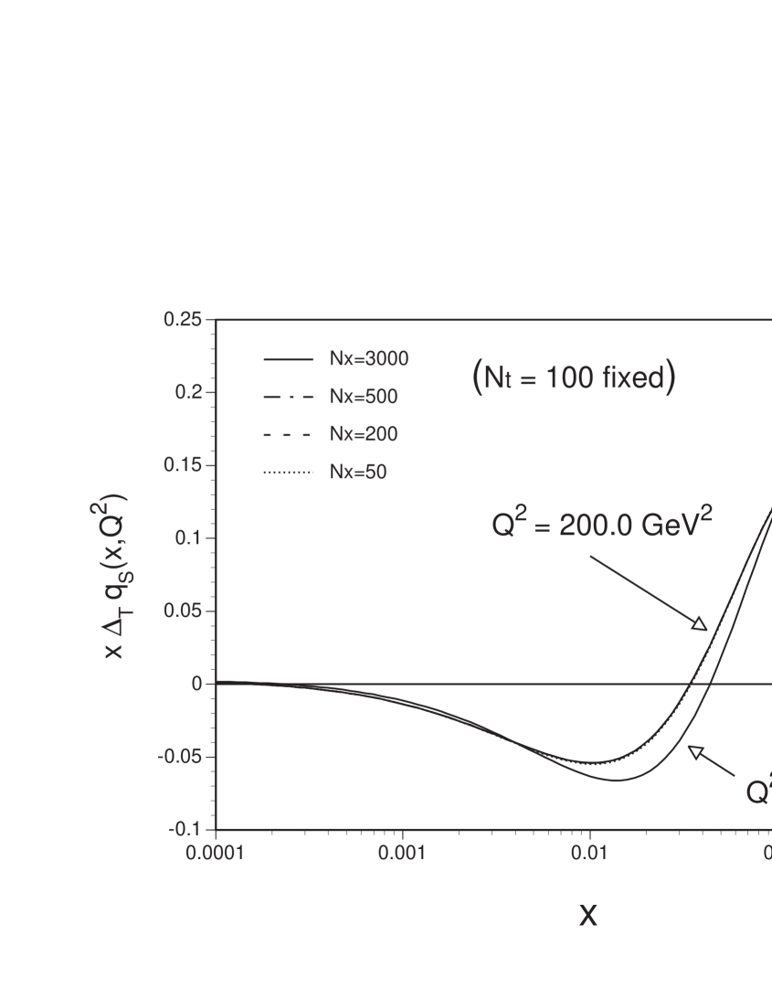
Figure 2: $N_{x}$ dependence of evolution results is shown for the singlet transversity distribution. The initial distribution is the same as the one in Fig. 1. $N_{t}$=100 is fixed and $N_{x}$ is varied as 50, 200, 500, and 1000. There are dotted, dashed, dot-dashed, and solid curves at $Q^{2}$=200 GeV² for $N_{x}$=50, 200, 500, and 1000 respectively.

Next, the step $N_{x}$ is varied with fixed $N_{t}$=100 in Fig. 2, where $N_{x}$=50, 200, 500, and 3000 are taken. Numerical accuracy is slightly worse in the $N_{x}$=50 case; however, the accurate results are obtained by taking the five hundred steps. Defining the evolution accuracy by $|\,[\Delta_{{}_{T}}q(N_{x},N_{t})-\Delta_{{}_{T}}q(N_{x}=3000,N_{t}=1000)]/\Delta_{{}_{T}}q(N_{x}=3000,N_{t}=1000)\,|$, we find that the accuracy is better than 1% in the region $10^{-5}<x<0.8$ with $N_{x}=500$ and $N_{t}=50$ in the logarithmic-$x$ steps (ILOG=2). If one is more interested in the large-$x$ region, one had better take the linear-$x$ steps (ILOG=1). However, we recommend the user to use the logarithmic steps in a general case.

Finally, we discuss a typical running CPU time. If one initial distribution is evolved with $N_{x}=500$ and $N_{t}=50$, it is about forty seconds on the AlphaServer 2100 4/200 and two and a half minutes on the SUN-IPX. From these analyses, we find that our program can be run on a typical workstation or possibly on a personal computer without spending much computing time. However, if one would like to calculate the evolution repeatedly or to evolve several distributions simultaneously, a reasonably powerful machine is recommended.

6.2 $\bf Q^{2}$ evolution of transversity distributions

There are some studies on the transversity evolution [11, 16, 17, 18]; however, it is not a well investigated topic. Therefore, we show evolution results of various transversity distributions in this subsection. In particular, the LO and NLO evolution differences are shown, then they are compared with those of the corresponding longitudinally polarized distributions by using the BFP1 program [20]. The transversity NLO evolution is the same in the $MS$ [12, 14] and $\overline{MS}$ [13] schemes.

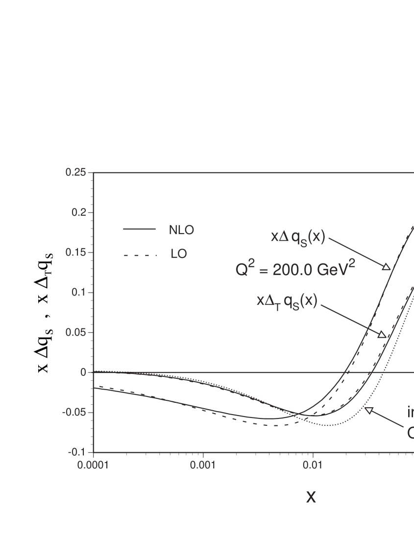
Figure 3: The singlet transversity evolution results are compared with those of longitudinally polarized singlet distribution. The longitudinal evolution is calculated by the BFP1 program [20]. The same GS-A distribution is assumed at $Q^{2}$=4 GeV², and it is shown by the dotted curve. It is evolved to the distributions at $Q^{2}$=200 GeV². The dashed and solid curves are the LO and NLO evolution results respectively.

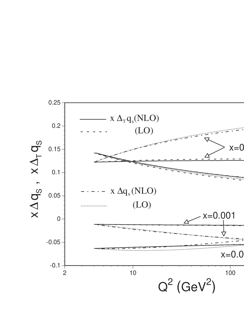
Figure 4: $Q^{2}$ dependent results of the transversity distribution are compared with those of the longitudinally polarized one. They are shown at $x$=0.001, 0.01, 0.1, and 0.5. The solid (dashed) curves are the NLO (LO) evolution results of $x\Delta_{{}_{T}}q_{s}$. The dot-dashed (dotted) curves are the NLO (LO) evolution results of $x\Delta q_{s}$.

First, the singlet evolution results are shown in Fig. 3. The same GS-A distribution is assumed for the transversity and longitudinally-polarized parton distributions at $Q^{2}$=4 GeV². Furthermore, the LO and NLO distributions are assumed the same in both cases. The initial distribution is shown by the dotted curve. It is evolved to the distributions at $Q^{2}$=200 GeV² by the transverse or longitudinal evolution equation. The transversity NLO effects increase the evolved distribution at medium-large $x$ and also at small $x$ ($<$0.01), and they decrease the distribution in the intermediate $x$ region ($0.01<x<0.1$). The NLO contributions are rather different from those of the longitudinal evolution. The transversity evolution differs significantly from the longitudinal one either in the LO case or in the NLO. The evolved transversity distribution $\Delta_{{}_{T}}q_{s}$ is significantly smaller than the longitudinal one $\Delta q_{s}$ in the region $x\sim 0.1$. The magnitude of $\Delta_{{}_{T}}q_{s}$ itself is also smaller than that of $\Delta q_{s}$ at very small $x$ ($<0.07$). Therefore, one should be careful about the $Q^{2}$ evolution difference between the two distributions in extracting information on $\Delta_{{}_{T}}q_{s}$ from experimental data. The explicit $Q^{2}$ dependence is shown in Fig. 4, where the distributions are shown at $x$=0.001, 0.01, 0.1, and 0.5.

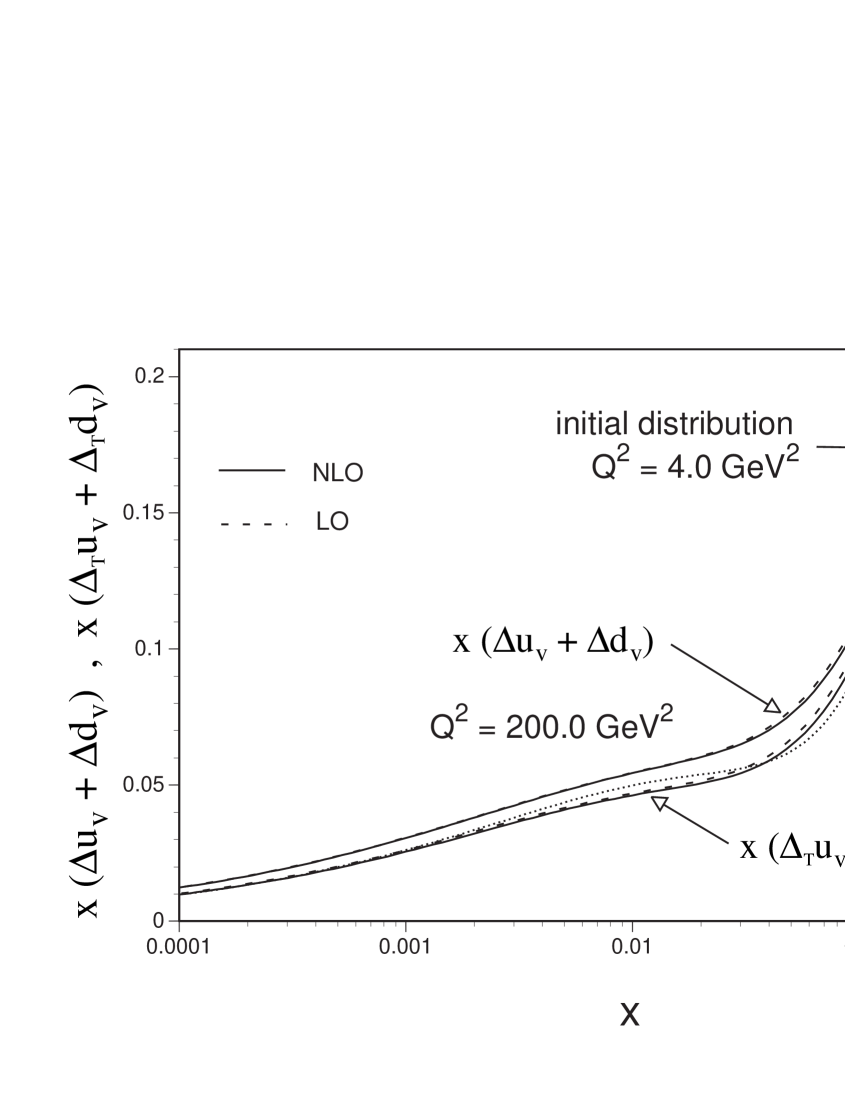
Figure 5: Evolution results of the valence-quark transversity distribution $x(\Delta_{{}_{T}}u_{v}+\Delta_{{}_{T}}d_{v})$ are compared with those of the longitudinally polarized one. The initial GS-A distribution at $Q^{2}$=4 GeV² is shown by the dotted curve, and it is evolved to the distributions at $Q^{2}$=200 GeV². The dashed and solid curves are the LO and NLO evolution results respectively.

In parametrizing the parton distributions [1], it is natural to provide the valence and sea quark distributions separately. We expect that future parametrizations on $\Delta_{{}_{T}}q_{s}$ will be given in the same manner. Therefore, it is important to show the evolution results of a valence-quark distribution. The evolution calculations are done in the same way as those in Fig. 3 except that the initial distribution is the nonsinglet one $x(\Delta u_{v}+\Delta d_{v})=x(\Delta_{{}_{T}}u_{v}+\Delta_{{}_{T}}d_{v})$. The evolution results are shown in Fig. 5. The dotted curve is the initial distribution, and evolved distributions are solid and dashed curves. The evolved transversity distributions are significantly smaller than the longitudinally polarized ones, in particular at small $x$.

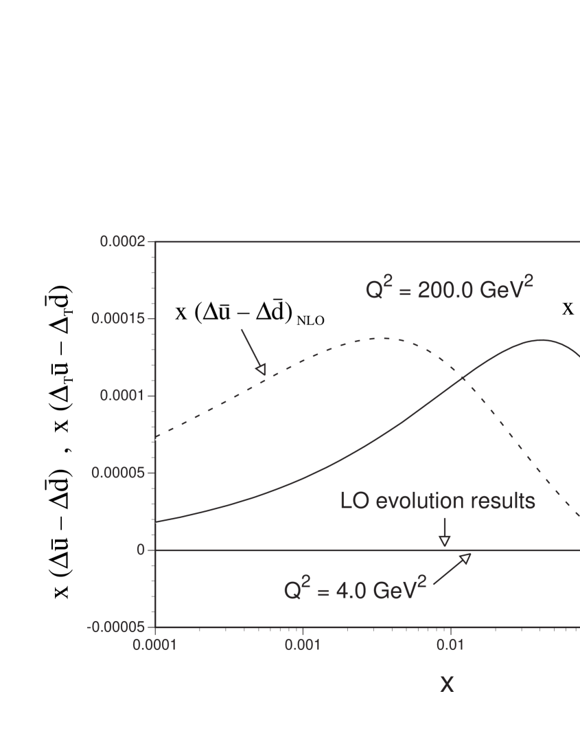
Figure 6: Evolution results of the flavor asymmetric transversity distribution $x(\Delta_{{}_{T}}\bar{u}-\Delta_{{}_{T}}\bar{d})$ are compared with those of the longitudinally polarized one. There is no flavor asymmetry in the initial GS-A distribution at $Q^{2}$=4 GeV² [$x(\Delta_{{}_{T}}\bar{u}-\Delta_{{}_{T}}\bar{d})$= $x(\Delta\bar{u}-\Delta\bar{d})$=0]. In the LO evolution, the evolved distributions are identically zero [$x(\Delta_{{}_{T}}\bar{u}-\Delta_{{}_{T}}\bar{d})_{LO}$= $x(\Delta\bar{u}-\Delta\bar{d})_{LO}$=0]. The NLO evolution results at $Q^{2}$=200 GeV² are shown by the solid and dashed curves for the $x(\Delta_{{}_{T}}\bar{u}-\Delta_{{}_{T}}\bar{d})$ and $x(\Delta\bar{u}-\Delta\bar{d})$ distributions respectively.

The other interesting distribution is the flavor asymmetric distribution $\Delta_{{}_{T}}\bar{u}-\Delta_{{}_{T}}\bar{d}$. Although the unpolarized version $\bar{u}-\bar{d}$ is rather well known [27] due to the measurements of the Gottfried-sum-rule violation and the Drell-Yan p-n asymmetry, the longitudinally polarized one $\Delta\bar{u}-\Delta\bar{d}$ is not investigated experimentally. Because of the difference between the splitting functions for the $\Delta_{{}_{T}}q+\Delta_{{}_{T}}\bar{q}$ and $\Delta_{{}_{T}}q-\Delta_{{}_{T}}\bar{q}$ type distributions, a finite $\Delta_{{}_{T}}\bar{u}-\Delta_{{}_{T}}\bar{d}$ could be obtained through the $Q^{2}$ evolution [18] as it appears also in the unpolarized case [27]. We show the evolution results of $\Delta_{{}_{T}}\bar{u}-\Delta_{{}_{T}}\bar{d}$ and $\Delta\bar{u}-\Delta\bar{d}$ in Fig. 6. As it is obvious from the figure, the obtained distributions are fairly small. In order to get the accurate evolution in Fig. 6, large numbers of $x$ and $t$ steps should be chosen: for example $N_{x}$=3000 and $N_{t}$=500. There is no flavor asymmetry in the GS-A antiquark distributions, so that the initial distributions are $\Delta_{{}_{T}}\bar{u}-\Delta_{{}_{T}}\bar{d}=\Delta\bar{u}-\Delta\bar{d}=0$. Because the difference between the $q^{\pm}$ splitting functions does not appear in the LO, the evolved distributions show no asymmetry $(\Delta_{{}_{T}}\bar{u}-\Delta_{{}_{T}}\bar{d})_{LO}=(\Delta\bar{u}-\Delta\bar{d})_{LO}=0$ at $Q^{2}$=200 GeV². The situation is completely different in the NLO. The NLO evolution results are shown by the solid and dashed curves. It is interesting to find the finite distributions in the NLO evolution. The evolved transversity distribution $x(\Delta_{{}_{T}}\bar{u}-\Delta_{{}_{T}}\bar{d})$ is concentrated in the $x\sim 0.04$ region, and the longitudinal one is distributed in the smaller $x$ ($\sim$0.004) region. However, we should note the magnitude. The distributions are typically 0.0001, which is too small to be found experimentally in the near future. The situation is the same in the unpolarized: the perturbative QCD correction to the Gottfried sum is typically 0.3% with respect to the 30% experimental violation. The $\Delta_{{}_{T}}\bar{u}-\Delta_{{}_{T}}\bar{d}$ as well as $\Delta\bar{u}-\Delta\bar{d}$ will be measured in the W-charge-asymmetry experiments at RHIC [28]. Even if finite distributions are found, they are unlikely to be explained by the perturbative mechanism.

7 Summary

We investigated numerical solution of the $Q^{2}$ evolution equation for the transversity distribution $\Delta_{{}_{T}}q$ or the structure function $h_{1}$. A useful FORTRAN program was created for calculating the evolution in the LO and NLO cases. The renormalization scheme is $MS$ or $\overline{MS}$ in the NLO. The numerical solution was obtained by dividing the variables $x$ and $t=\ln\,Q^{2}$ into small steps with the numbers of steps, $N_{x}$ and $N_{t}$. The Euler and Simpson methods are used for solving the integrodifferential equation. We find that the evolution accuracy is better than 1% with $N_{x}\geq 500$ and $N_{t}\geq 50$ in the $x$ region $10^{-5}<x<0.8$  .

Using the program, we showed the evolution results of the valence-quark distribution $x(\Delta_{{}_{T}}u_{v}+\Delta_{{}_{T}}d_{v})$, the singlet distribution $x\sum_{i}^{N_{f}}(\Delta_{{}_{T}}q_{i}+\Delta_{{}_{T}}\bar{q}_{i})$, and the flavor asymmetric distribution $x(\Delta_{{}_{T}}\bar{u}-\Delta_{{}_{T}}\bar{d})$. The evolution results are compared with those calculated by the longitudinal DGLAP evolution equations. Because the transverse and longitudinal evolution results are significantly different, we should be careful in analyzing experimental data. The $Q^{2}$ variations of the flavor asymmetric distribution are fairly small so that a nonperturbative mechanism should be explored if a finite distribution is found experimentally. The transversity evolution of these distributions should be tested by future experimental projects such as the RHIC-Spin.

Appendix A. Splitting functions and running
                  coupling constants

The running coupling constant in the leading order (LO) is given by

$$\alpha_{s}^{LO}(Q^{2})=\frac{4\pi}{\beta_{0}\ln(Q^{2}/\Lambda^{2})}\ ,$$ (A.1)

and the one in the next-to-leading order (NLO) is

$$\alpha_{s}^{NLO}(Q^{2})=\frac{4\pi}{\beta_{0}\ln(Q^{2}/\Lambda^{2})}\left[1-\frac{\beta_{1}\ln\{\ln(Q^{2}/\Lambda^{2})\}}{\beta_{0}^{2}\ln(Q^{2}/\Lambda^{2})}\right]\ .$$ (A.2)

The constants $\beta_{0}$ and $\beta_{1}$ are defined by the color constants $C_{G}$, $C_{F}$, and $T_{R}$ as

$$\beta_{0}=\frac{11}{3}C_{G}-\frac{4}{3}T_{R}N_{f}\ ,\ \ \ \ \beta_{1}=\frac{34}{3}C^{2}_{G}-\frac{10}{3}C_{G}N_{f}-2C_{F}N_{f}\ ,$$ (A.3)

where

$$C_{G}=N_{c}\ ,\ \ \ C_{F}=\frac{N_{c}^{2}-1}{2N_{c}}\ ,\ \ \ T_{R}=\frac{1}{2}\ ,$$ (A.4)

with the number of color ($N_{c}$=3) and the number of flavor ($N_{f}$).

The splitting function is expressed by the LO and NLO splitting functions as

$$\Delta_{{}_{T}}P_{q^{\pm}}(x)=\Delta_{{}_{T}}P_{qq}^{(0)}(x)+\frac{\alpha_{s}(Q^{2})}{2\pi}\,\Delta_{{}_{T}}P_{q^{\pm}}^{(1)}(x)\ .$$ (A.5)

The second term is the NLO contribution. We use the expressions in Ref. [13] for the transversity splitting functions. The LO splitting function is given by [10]

$$\Delta_{T}P_{qq}^{(0)}(x)=C_{F}\Bigg{[}\frac{2\,x}{(1-x)_{+}}+\frac{3}{2}\,\delta(1-x)\Bigg{]}\ ,$$ (A.6)

where the ‘+’ function is defined by

$$\int_{0}^{1}dz\,{\frac{f(z)}{(1-z)_{+}}}\ =\ \int_{0}^{1}dz\,{\frac{f(z)-f(1)}{1-z}}\ .$$ (A.7)

It should be noted that the above integration is defined in the region $0\leq z\leq 1$. However, the integration is given in the region $x\leq z\leq 1$ in the actual evolution calculation. In such a case, the integral with ‘+’ function is calculated by the following equation:

$$\int_{x}^{1}dz\,{\frac{f(z)}{(1-z)_{+}}}\ =\ \int_{x}^{1}dz\,{\frac{f(z)-f(1)}{1-z}}\ +\ f(1)\ln(1-x)\ .$$ (A.8)

The NLO splitting function is [13]

$$\Delta_{T}P_{q^{\pm}}^{(1)}(x) \equiv\Delta_{T}P_{qq}^{(1)}(x)\pm\Delta_{T}P_{q\bar{q}}^{(1)}(x)\ ,$$ (A.9)

$$\Delta_{T}P_{qq}^{(1)}(x) =C_{F}^{2}\Bigg{[}1-x-\left(\frac{3}{2}+2\ln(1-x)\right)\ln x\;\delta_{T}P_{qq}^{(0)}(x)$$

$$\!\!\!\!\!\!\!\!\!\!\!\!\!\!\!\!\!\!\!\!\!\!\!\!\!\!\!+\left.\left(\frac{3}{8}-\frac{\pi^{2}}{2}+6\zeta(3)\right)\delta(1-x)\right]+\frac{1}{2}C_{F}C_{G}\bigg{[}-(1-x)$$

$$\!\!\!\!\!\!\!\!\!\!\!\!\!\!\!\!\!\!\!\!\!\!\!\!\!\!\!\left.+\left(\frac{67}{9}+\frac{11}{3}\ln x+\ln^{2}x-\frac{\pi^{2}}{3}\right)\delta_{T}P_{qq}^{(0)}(x)+\left(\frac{17}{12}+\frac{11\pi^{2}}{9}-6\zeta(3)\right)\delta(1-x)\right]$$

$$\!\!\!\!\!\!\!\!\!\!\!\!\!\!\!\!\!\!\!\!\!\!\!\!\!\!\!+\frac{2}{3}C_{F}T_{R}N_{f}\left[\left(-\ln x-\frac{5}{3}\right)\delta_{T}P_{qq}^{(0)}(x)-\left(\frac{1}{4}+\frac{\pi^{2}}{3}\right)\delta(1-x)\right]\ ,$$ (A.10)

$$\Delta_{T}P_{q\bar{q}}^{(1)}(x) =C_{F}\left(C_{F}-\frac{1}{2}C_{G}\right)\Bigg{[}-(1-x)+2S_{2}(x)\,\delta_{T}P_{qq}^{(0)}(-x)\Bigg{]}\ ,$$ (A.11)

where $\delta_{T}P_{qq}^{(0)}(x)=2x/(1-x)_{+}$. The $\zeta$ function is defined by $\zeta(k)=\sum_{n=1}^{\infty}1/n^{k}$, and $\zeta(3)$ is given by the numerical value ($\zeta(3)$=1.2020569…). The $\pm$ factor in Eq. (A.9) indicates “$\Delta_{{}_{T}}q\pm\Delta_{{}_{T}}\bar{q}$ type” distribution $\sum_{i}a_{i}(\Delta_{{}_{T}}q_{i}\pm\Delta_{{}_{T}}\bar{q}_{i})$. The $S_{2}$ function is expressed in terms of the Spence function $S(x)$ as

$$S_{2}(x) \equiv\int_{x/(1+x)}^{1/(1+x)}\frac{dz}{z}\ln{\frac{1-z}{z}}$$

$$=S\left({\frac{x}{1+x}}\right)-S\left({\frac{1}{1+x}}\right)-\frac{1}{2}\left[\ln^{2}\frac{1}{1+x}-\ln^{2}\frac{x}{1+x}\right]\ ,$$ (A.12)

where $S(x)$ is defined by

$$S(x)\,=\,\int_{x}^{1}dz\,\frac{\ln z}{1-z}\ .$$ (A.13)

The NLO splitting function or anomalous dimensions are the same in the $MS$ scheme [12, 14] and in the $\overline{MS}$ scheme [13]. Therefore, our evolution program can be used in both schemes.

TEST RUN OUTPUT

IOUT= 1   IREAD= 1   INDIST= 1   IORDER= 2   IMORP= 2   ILOG= 2
Q02= 4.0000   Q2= 200.000   DLAM= 0.2310   NF= 4   NFI= 1
XX= 0.1000000   NX= 500   NT= 50   NSTEP= 50   XMIN= 0.0001000

0.000100	0.001041
0.000120	0.000710
0.000145	0.000292
0.000174	–0.000226
0.000209	–0.000860
0.000251	–0.001628
0.000302	–0.002547
0.000363	–0.003638
0.000437	–0.004921
0.000525	–0.006418
0.000631	–0.008149
0.000759	–0.010137
0.000912	–0.012398
0.001096	–0.014949
0.001318	–0.017798
0.001585	–0.020945
0.001905	–0.024379
0.002291	–0.028073
0.002754	–0.031979
0.003311	–0.036023
0.003981	–0.040097
0.004786	–0.044055
0.005754	–0.047704
0.006918	–0.050799
0.008318	–0.053040
0.010000	–0.054072
0.012023	–0.053492
0.014454	–0.050863
0.017378	–0.045742
0.020893	–0.037724
0.025119	–0.026499
0.030200	–0.011925
0.036308	0.005892
0.043652	0.026521
0.052481	0.049165
0.063096	0.072675
0.075858	0.095662
0.091201	0.116708
0.109648	0.134650
0.131826	0.148836
0.158489	0.159176
0.190546	0.165818
0.229087	0.168430
0.275423	0.165410
0.331131	0.153773
0.398107	0.130477
0.478630	0.095291
0.575440	0.053977
0.691831	0.018859
0.831764	0.001962
1.000000	0.000000

Figures

Figure 1: $N_{t}$ dependence of evolution results is shown for the singlet transversity distribution. The initial distribution is assumed to be the longitudinally polarized GS-A distribution at Q²=4 GeV². It is evolved to the one at Q²=200 GeV² by the next-to-leading-order DGLAP evolution equation with $\Lambda_{QCD}$=231 MeV and $N_{f}$=4. $N_{x}$=1000 is fixed and $N_{t}$ is varied as 10, 50, 200, and 1000. There are dotted, dashed, dot-dashed, and solid curves at $Q^{2}$=200 GeV² for $N_{t}$=10, 50, 200, and 1000 respectively.

References

- [1] RHIC-SPIN-J working group on parametrization: Y. Goto, N. Hayashi, M. Hirai, H. Horikawa S. Kumano, M. Miyama, T. Morii, N. Saito, T.-A. Shibata, E. Taniguchi, and T. Yamanishi, research in progress.
- [2] J. P. Ralston and D. E. Soper, Nucl. Phys. B152 (1979) 109.
- [3] R. L. Jaffe and X. Ji, Phys. Rev. Lett. 67 (1991) 552; Nucl. Phys. B375 (1992) 527; X. Ji, Phys. Lett. B284 (1992) 137.
- [4] J. L. Cortes, B. Pire, and J. P. Ralston, Z. Phys. C55 (1992) 409; J. C. Collins, S. F. Heppelmann, and G. A. Ladinsky, Nucl. Phys. B420 (1994) 565; B. Kamal, Phys. Rev. D53 (1996) 1142; R. L. Jaffe and N. Saito, Phys. Lett. B382 (1996) 165.
- [5] Proposal on Spin Physics Using the RHIC Polarized Collider (RHIC-Spin collaboration), August 1992; update, Sept. 2, 1993.
- [6] P. J. Mulders and R. D. Tangerman, Nucl. Phys. B461 (1996) 197.
- [7] B. L. Ioffe and A. Khodjamirian, Phys. Rev. D51 (1995) 3373; J. Soffer, Phys. Rev. Lett. 74 (1995) 1292; S. Aoki, M. Doui, T. Hatsuda, and Y. Kuramashi, Phys. Rev. D56 (1997) 433; A. Y. Umnikov, H. He, and F. C. Khanna, Phys. Lett. B398 (1997) 6; R. Kirschner, L. Mankiewicz, A. Schäfer, and L. Szymanowski, Z. Phys. C74 (1997) 501; M. Meyer-Hermann and A. Schäfer, hep-ph/9709349; K. Suzuki and T. Shigetani, hep-ph/9709394; R. L. Jaffe, X. Jin, and J. Tang, hep-ph/9709322.
- [8] M. Göckeler, R. Horsley, H. Perlt, P. Rakow, G. Schierholz, A. Schiller, and P. Stephenson, hep-ph/9711245.
- [9] V. N. Gribov and L. N. Lipatov, Sov. J. Nucl. Phys. 15 (1972) 438 and 675; G. Altarelli and G. Parisi, Nucl. Phys. B 126 (1977) 298; Yu. L. Dokshitzer, Sov. Phys. JETP 46 (1977) 641.
- [10] X. Artru and M. Mekhfi, Z. Phys. C45 (1990) 669.
- [11] V. Barone, T. Calarco, and A. Drago, Phys. Lett. B390 (1997) 287.
- [12] S. Kumano and M. Miyama, Phys. Rev. D56 (1997) 2504.
- [13] W. Vogelsang, hep-ph/9706511, Phys. Rev. D in press.
- [14] A. Hayashigaki, Y. Kanazawa, and Y. Koike, hep-ph/9707208, Phys. Rev. D in press; numerical analysis in progress.
- [15] The NLO evolution was first reported in Ref. [12] as the Los Alamos preprint hep-ph/9706420. The first version had some typing and calculation mistakes. The correct final result was reported in the subsequent preprint hep-ph/9707208 [14] within the same formalism as well as in Ref. [12].
- [16] S. Scopetta and V. Vento, hep-ph/9707250.
- [17] C. Bourrely, J. Soffer, and O. V. Teryaev, hep-ph/9710224.
- [18] O. Martin, A. Schäfer, M. Stratmann, and W. Vogelsang, hep-ph/9710300.
- [19] G. P. Ramsey, J. Comput. Phys. 60 (1985) 97; J. Blümlein, G. Ingelman, M. Klein, and R. Rückl, Z. Phys. C 45 (1990) 501; S. Kumano and J. T. Londergan, Comput. Phys. Commun. 69 (1992) 373; R. Kobayashi, M. Konuma, and S. Kumano, Comput. Phys. Commun. 86 (1995) 264.
- [20] M. Miyama and S. Kumano, Comput. Phys. Commun. 94 (1996) 185; M. Hirai, S. Kumano, and M. Miyama, hep-ph/9707220, Comput. Phys. Commun. in press.
- [21] J. Blümlein, B. Geyer, and D. Robaschik, hep-ph/9711405.
- [22] B. Carnahan, H. A. Luther, and J. O. Wilkes, Applied Numerical Methods (John Wiley & Sons, 1969).
- [23] T. Gehrmann and W. J. Stirling, Phys. Rev. D. 53 (1996) 6100.
- [24] G. E. Forsythe, M. A. Malcolm, and C. B. Moler, Computer Methods for Mathematical Computations (Prentice-Hall, 1977).
- [25] B.-Q. Ma, I. Schmidt, and J. Soffer, hep-ph/9710247.
- [26] M. Glück, E. Reya, M. Stratmann, and W. Vogelsang, Phys. Rev. D53 (1996) 4775.
- [27] S. Kumano, hep-ph/9702367.
- [28] N. Saito, pp.40–49 in Spin Structure of the Nucleon, edited by T.-A. Shibata, S. Ohta, and N. Saito, (World Scientific, 1996); J. Soffer and J.-M. Virey, hep-ph/9706229; B. Kamal, hep-ph/9710374.