NEW RESULTS IN VECTOR MESON DOMINANCE AND RHO MESON PHYSICS

Abstract

Recent results by Benayoun et al. comparing the predictions of a range of existing models based on the Vector Meson Dominance hypothesis are summarized and discussed. These are compared with data on $e^{+}e^{-}\rightarrow\pi^{+}\pi^{-}$ and $e^{+}e^{-}\rightarrow\mu^{+}\mu^{-}$ cross-sections and the phase and near-threshold behavior of the timelike pion form factor, with the aim of determining which (if any) of these models is capable of providing an accurate representation of the full range of experimental data. We find that, of the models considered, only Hidden Local Symmetry (HLS) model proposed by Bando et al. is able to consistently account for all information, provided one allows its parameter $a$ to vary from the usual value of 2 to 2.4. Our fit with the HLS model gives a point–like coupling $\gamma\pi^{+}\pi^{-}$ of magnitude $\simeq-e/6$, while the common formulation of VMD excludes such a term. The resulting values for the $\rho$ mass and $\pi^{+}\pi^{-}$ and $e^{+}e^{-}$ partial widths as well as the branching ratio for the decay $\omega\rightarrow\pi^{+}\pi^{-}$ obtained within the context of this model are consistent with previous results.

1 Introduction.

A recent detailed study [2] by Benayoun et al. of a variety of models of vector meson dominance and associated descriptions of the $\rho^{0}$ meson is reviewed and summarized. The aim is to find an optimum modelling able to account most precisely for the known features of the physics involving this meson. It is important to emphasise that our philosophy is to look for the simplest models as these are the most useful in application to other systems, due to their ease of implementation. Naturally, such models should, as much as possible, respect basic general principles such as gauge invariance and unitarity. One must keep in mind that any parameters quoted for a given model are relevant only to that model. Indeed, a study of the model-dependence of resonance parameters is one of the principal goals of this work.

We study the strong interaction corrections to one-photon mediated processes in the low energy region where QCD is non-perturbative. To do this we shall look at two related processes, $e^{+}e^{-}\rightarrow\pi^{+}\pi^{-}\;$and $e^{+}e^{-}\rightarrow\mu^{+}\mu^{-}\;$. The effect of the strong interaction is obvious in the first reaction and provides a large enhancement to the production of pions in the vector meson resonance region [3, 4, 5, 6]. This enhancement, relative to what would be expected for a structureless, pointlike pion, is reflected in the deviation of the pion form factor, $F_{\pi}(q^{2})$, from $1$, and is primarily associated with the $\rho$ meson (where $q_{\mu}$ is the four momentum of the virtual photon). This form factor is successfully modelled in the intermediate energy region using the vector meson dominance (VMD) model [7]. VMD assumes that the photon interacts with physical hadrons through vector mesons and it is these mesons that give rise to the enhancement, through their resonant (possessing a complex pole) propagators of the form

$$D_{\mu\nu}(q^{2})=\frac{-g_{\mu\nu}}{q^{2}-{m}_{V}^{2}+i{m}_{V}\Gamma_{V}(q^{2})},$$ (1)

where ${m}_{V}$ and $\Gamma_{V}$ are the (real valued) mass and the momentum-dependent width. (Here we have included only that part of the propagator which survives when coupled to conserved currents.)

Traditionally, VMD assumes that all photon–hadron coupling is mediated by vector mesons. However, from an empirical point of view, one has the freedom, motivated by Chiral Perturbation Theory (ChPT) to include other contributions to such interactions. The values extracted from $F_{\pi}(q^{2})$ for the $\rho$ mass, $m_{\rho}$, and width, $\Gamma_{\rho}$, are model-dependent and in quoting values for them, the model used should be clearly stated.

We thus turn our attention to $e^{+}e^{-}\rightarrow\mu^{+}\mu^{-}\;$. In modelling the strong interaction correction to the photon propagator, VMD assumes that the strong interaction contribution is saturated by the spectrum of vector meson resonances [8]. Therefore, in principle, we can extract information on the vector meson parameters (independently of the $e^{+}e^{-}\rightarrow\pi^{+}\pi^{-}\;$fit) without having to worry about non-resonant processes. However, as the vector mesons enter in $e^{+}e^{-}\rightarrow\mu^{+}\mu^{-}\;$with an extra factor of $\alpha$ compared with $e^{+}e^{-}\rightarrow\pi^{+}\pi^{-}\;$, their contributions are considerably suppressed, making their extraction difficult. For this reason, we shall perform a simultaneous fit to both sets of data, in order to impose the best possible constraint on the vector meson parameters, and see if existing muon data are already precise enough in order to constrain the $\rho^{0}$ parametrisation.

Another way to constrain the descriptions of the $\rho^{0}$ meson is to compare the strong interaction $\pi\pi$ phase obtained using the various VMD parametrisations determined in fitting $e^{+}e^{-}\rightarrow\pi^{+}\pi^{-}\;$with the corresponding phase [9] obtained using $\pi\pi$ scattering data and the general principles of quantum field theory, as well as the near–threshold predictions of ChPT. This happens to be more fruitful and conclusive in showing how VMD should be dealt with in order to reach an agreement with a large set of data and with the basic principles of quantum field theory.

2 Vector meson models

We shall now provide a description of the various models we will use to fit the data for both $e^{+}e^{-}\rightarrow\pi^{+}\pi^{-}\;$and $e^{+}e^{-}\rightarrow\mu^{+}\mu^{-}\;$. The cross-section for $e^{+}e^{-}\rightarrow\pi^{+}\pi^{-}\;$is given by (neglecting the electron mass)

$$\sigma=\frac{\pi\alpha^{2}}{3}\frac{(q^{2}-4m_{\pi}^{2})^{3/2}}{(q^{2})^{5/2}}|F_{\pi}(q^{2})|^{2},$$ (2)

where the form factor, $F_{\pi}(q^{2})$ is determined by the specific model. Similarly, $F_{\mu}(q^{2})$ is defined to be the form factor for the muon, and the cross-section for $e^{+}e^{-}\rightarrow\mu^{+}\mu^{-}\;$is given by,

$$\sigma=\frac{4\pi\alpha^{2}}{3q^{2}}\sqrt{1-\frac{4m_{\mu}^{2}}{q^{2}}}\left(1+\frac{2m_{\mu}^{2}}{q^{2}}\right)|F_{\mu}(q^{2})|^{2}.$$ (3)

It is worth noting that these standard definitions of $F_{\pi}(q^{2})$ and $F_{\mu}(q^{2})$ contain all non-perturbative effects, including for example the photon vacuum polarisation, since Eqs. (2) and (3) are written assuming a perturbative photon propagator.

We shall use VMD, the Hidden Local Symmetry (HLS) model [10] and what we will refer to as the WCCZW model (a phenomenological modification of the general framework of Ref. [11], based on work by Birse[12]), as well as modifications of these models, which cover or underlie a large class of effective Lagrangians describing the interactions of photons, leptons and pseudoscalar and vector mesons. Birse [12] has shown that typical effective theories involving vector mesons based on a Lagrangian approach, such as “massive Yang-Mills” and “hidden gauge” (i.e., HLS-type) are equivalent. We therefore consider our following examination to be reasonably comprehensive. Numerical approaches to the strong interaction in the vector meson energy region [13], which are not based on an effective Lagrangian involving meson degrees of freedom do not yet possess the required calculational accuracy for our task.

2.1 VMD

The simplest model is VMD itself. As has been discussed in detail elsewhere [7, 14, 15] VMD has two equivalent formulations, which we shall call VMD1 and VMD2. The VMD1 model has a momentum-dependent coupling between the photon and the vector mesons and a direct coupling of the photon to the hadronic final state. The resulting form factor is (to leading order in isospin violation and $\alpha=e^{2}/4\pi$):

$$F_{\pi}^{\rm VMD1}(q^{2}) = 1-g^{\rm VMD1}_{\rho\gamma}(q^{2})\frac{g_{\rho\pi\pi}}{[q^{2}-m^{2}_{\rho}+im_{\rho}\Gamma_{\rho}(q^{2})]}$$ (4)

$$-g^{\rm VMD1}_{\omega\gamma}(q^{2})\frac{1}{[q^{2}-m^{2}_{\omega}+im_{\omega}\Gamma_{\omega}(q^{2})]}Ae^{i\phi_{1}}.$$

The $\omega$ enters into the isospin 1 $e^{+}e^{-}\rightarrow\pi^{+}\pi^{-}\;$interaction with an attenuation factor specified by the pure real $A$ and the Orsay phase, $\phi$ [16]; these can be extracted from experiment For VMD2 we have,

$$F_{\pi}^{\rm VMD2}(q^{2})=-g^{\rm VMD2}_{\rho\gamma}\frac{g_{\rho\pi\pi}}{[q^{2}-m^{2}_{\rho}+im_{\rho}\Gamma_{\rho}(q^{2})]}-g^{\rm VMD2}_{\omega\gamma}\frac{1}{[q^{2}-m^{2}_{\omega}+im_{\omega}\Gamma_{\omega}(q^{2})]}Ae^{i\phi_{2}}.$$ (5)

The form factor for the muon, however, in both representations (i=1, 2) is given by

$$F_{\mu}^{\rm VMDi}=1+\sum_{V}e^{2}[g_{V\gamma}^{\rm VMDi}(q^{2})]^{2}\frac{1}{q^{2}-{m}_{V}^{2}+i{m}_{V}\Gamma_{V}(q^{2})}\frac{1}{q^{2}},$$ (6)

which is consistent with previous expressions for the $\phi$-meson [3, 17]. In higher order (i.e., in all but the minimal VMD picture) there will also be contributions from non–resonant processes (such as two–pion loops), but these are expected to be small near resonance and the non–resonant background is, in any case, fitted in extractions of resonance parameters from the experimental data. The photon–meson coupling, $eg_{V\gamma}$ is fixed in VMD2 by [17]

$$\Gamma_{V\rightarrow e^{+}e^{-}}=\frac{4\pi\alpha^{2}}{3{m}_{V}^{3}}g^{2}_{V\gamma}.$$ (7)

The (dimensionless) universality coupling, $g_{V}$, is then defined by

$$g_{V\gamma}^{\rm VMD2}={m}_{V}^{2}/g_{V}$$ (8)

for VMD2 [14, 16]. This coupling (and universality) has been most closely studied for the $\rho$ meson. A gauge-like argument [7, 18] suggests that the $\rho$ couples to all hadrons with the same strength $g_{V}$ (universality) [14]. However, experimentally, universality is observed to be not quite exact [19], so we introduce the quantity $\epsilon$ (to be fitted) through

$$g_{\rho\gamma}^{\rm VMD2}=\frac{{m}_{\rho}^{2}}{g_{\rho\pi\pi}}(1+\epsilon)$$ (9)

where $g_{\rho\pi\pi}$ and $\epsilon$ are to be extracted from the fit to $e^{+}e^{-}\rightarrow\pi^{+}\pi^{-}\;$. For VMD1, it can be seen that the photon-meson coupling results from replacing the mass term in Eq. (8) by $q^{2}$ (see Ref.[7, 18]). In this case Eq (9) should be replaced by

$$g_{V\gamma}^{\rm VMD1}=\frac{q^{2}}{g_{\rho\pi\pi}}(1+\epsilon)~{}~{}.$$ (10)

One can easily see that in VMD1 the hadronic correction to the photon propagator goes like $q^{4}$ and so maintains the photon pole at $q^{2}=0$. For VMD2, it is not obvious [20] that gauge invariance is maintained until one considers the inclusion of a bare photon mass term in the VMD Lagrangian that exactly cancels the hadronic correction at $q^{2}=0$. This argument [21] assumes a $\rho-\gamma$ coupling of the form $em_{\rho}^{2}/g_{\rho}$ and a bare photon mass ($e^{2}m_{\rho}^{2}/g_{\rho}^{2}$) (the calculation is presented in detail in Ref. [7]). In the presence of a finite $\epsilon$, as in Eq. (9), gauge invariance is similarly preserved by including a photon mass term ($e^{2}m_{\rho}^{2}(1+\epsilon)^{2}/g_{\rho}^{2}$) leading to a massless photon as expected [22].

The presence of a finite $\epsilon$ does affect the charge normalisation condition $F_{\pi}(0)=1$, but this is merely an artifact of the simple $\rho$ propagators we are considering. A more sophisticated version, such as used by Gounaris and Sakurai [23] which fully accounts for below threshold behaviour, maintains $F_{\pi}(0)=1$ in the presence of $\epsilon\neq 0$. One could, alternatively, include an $s$ dependence to $\epsilon$ such that $\epsilon(0)=0$. In any case, the phenomenological significance for the physical $\rho$ (for the data region we are fitting) is negligible, we achieve an excellent fit to the data with the simple form we use but are not advocating its use outside this fitting region, namely above the two-pion threshold.

The choice of the detailed form of the momentum-dependent width, $\Gamma_{V}(q^{2})$, allows one certain amount of freedom. As the complex poles of the amplitude are field-choice and process-independent properties of the S-matrix [24] one could, on the one hand, expand the propagator as a Laurent series in which the non-pole terms go into the background [25]. Alternatively, one could use the $l-$wave momentum-dependent width to account for the branch point structure of the propagator above threshold ($q^{2}=4m_{\pi}^{2}$) [27, 23, 26]. This form for the momentum dependent width arises naturally from the dressing of the $\rho$ propagator in an appropriate Lagrangian based model (see Sec. 5.1 of Klingl et al. for a detailed treatment [19]) and, for such models, is given by

$$\Gamma_{\rho}(q^{2})=\Gamma_{\rho}\left[\frac{p_{\pi}(q^{2})}{p_{\pi}(m_{\rho}^{2})}\right]^{3}\left[\frac{m_{\rho}^{2}}{q^{2}}\right]^{\lambda/2},$$ (11)

introducing the fitting parameters $\Gamma_{\rho}$ (the width of the $\rho^{0}$ meson at $q^{2}=m_{\rho}^{2}$) and $\lambda$, which generalises the usual $l$–wave expression [27] to model the fall–off of the $\rho$ mass distribution; the usual case (i.e. $\lambda=1$) is associated with a $\rho$ coupling to pions of the form $g_{\rho\pi\pi}\rho^{\mu}(\pi^{+}\partial_{\mu}\pi^{-}-\pi^{-}\partial_{\mu}\pi^{+})$, with $g_{\rho\pi\pi}$ independent of $q^{2}$, as shown in Ref. [19]. Note that the parameters $\lambda$, $m_{\rho}$ and $\Gamma_{\rho}$ are model-dependent (as we see in the tables of results, different models yield different values for these parameters). Note that in Eq. (11) we have defined the pion momentum in the centre of mass system

$$p_{\pi}(q^{2})=\frac{1}{2}\sqrt{q^{2}-4m_{\pi}^{2}}.$$ (12)

Before closing this section, let us remark that the pion form factor associated with VMD1 (Eq. (4)) fulfills automatically the condition $F_{\pi}(0)=1$ whatever the value of the universality violating parameter $\epsilon$ (see Eq. (10)). This is not the case for the pion form factor associated with VMD2 (Eq. (5)), as can be seen from Eqs. (5) and (9). Here, we will concern ourselves exclusively with fitting data in the above threshold region and simply note it is a relatively straightforward matter to generalise the VMD models considered to satisfy this condition. Detailed considerations of this issue are left for future work.

While of course VMD1 and VMD2 are equivalent in the limit of exact universality if one keeps all diagrams, (i.e., if one works to infinite order in perturbation theory), in any practical calculation one cannot do that and so, in practice, these two expressions of VMD can give different predictions in general, even if exact universality is imposed. Moreover, if one releases (as we do) this last constraint, equivalence of VMD1 and VMD2 is not guaranted, even in principle.

2.2 The Hidden Local Symmetry Model

The HLS model [7, 10] introduces a parameter $a$ for the $\rho$ meson within a dynamical symmetry breaking model framework. This $a$ relates the constant $g_{\rho\pi\pi}$ to the universality coupling $g_{\rho}$ via

$$g_{\rho\pi\pi}=\frac{ag_{\rho}}{2}.$$ (13)

The resulting form factor for the pion is

$$F_{\pi}(q^{2})=-\frac{a}{2}+1-g_{\rho\gamma}\frac{g_{\rho\pi\pi}}{(q^{2}-m_{\rho}^{2}+im_{\rho}\Gamma_{\rho}(q^{2}))}-g_{\omega\gamma}\frac{1}{q^{2}-m^{2}_{\omega}+im_{\omega}\Gamma_{\omega}(q^{2})}Ae^{i\phi}.\\$$ (14)

The original HLS model preserved isospin symmetry and so did not include the $\omega$. Isospin breaking has recently been studied in a generalisation of the HLS model [28], however, here we have for simplicity employed the same $\omega$ terms as used for VMD. The relations equivalent to Eqs. (8) and (9) for the $\rho$ meson are now

$$g_{\rho\gamma}=\frac{a}{2}\frac{m_{\rho}^{2}}{g_{\rho\pi\pi}}=\frac{m_{\rho}^{2}}{g_{\rho}}\ .$$ (15)

We see that setting $a=2$ reproduces VMD2 in the limit of exact universality. However, we wish to keep $a$ as a free parameter which we can fit to the data. Note that in the HLS model universality violation and the existence of a non–resonant coupling $\gamma\pi^{+}\pi^{-}$ are related. Note also that universality violation can be introduced in the HLS model without violating the constraint $F_{\pi}(0)=1$, in a natural way.

The muon form factor for the HLS model is exactly the same as for VMD2 (see Eqs. (6) and (15)).

2.3 WCCWZ Lagrangian

Birse has recently discussed [12] the pion form factor arising from the WCCWZ Lagrangian [11] in which the vector and axial vector fields transform homogeneously under non-linear chiral symmetry. The scheme imposes no constraints on the couplings of the spin 1 particles beyond those of approximate chiral symmetry. Birse’s version of the form factor is (isospin violation is not considered)

$$F_{\pi}(q^{2})=1-\frac{g_{1}f_{1}}{f_{\pi}^{2}}\frac{q^{4}}{q^{2}-m^{2}_{\rho}+im_{\rho}\Gamma_{\rho}(q^{2})}+\frac{f_{2}}{f_{\pi}^{2}}q^{2},$$ (16)

where the first two terms on the RHS are those arising from the WCCWZ Lagrangian. The $q^{4}$ piece grows at large $q^{2}$ in a way incompatible with QCD predictions (for a discussion of matching the asymptotic prediction to a low energy model see Geshkenbein [29]). The $f_{2}$ contribution has been added by Birse to modify this high energy behaviour toward that expected in QCD. To this end, Birse sets

$$f_{2}=g_{1}f_{1}=\frac{f_{\pi}^{2}}{m^{2}_{\rho}}$$ (17)

and recovers the universality limit of the form factor in which VMD1 and VMD2 are equivalent (in the zero width approximation). Note that a $q^{2}$-dependence of the non-resonant background is what one would, in general, obtain from the WCCWZ framework, implemented in its most general form, which relies only on the symmetries of QCD. In constructing a phenomenological implementation we have, however, simplified the most general form, adding what amounts to a minimal $q^{2}$-dependence to the background term of VMD1. The resulting form factor, which we will refer to as the WCCWZ model, is then

$$F_{\pi}(q^{2})=1+bq^{2}-\frac{g_{\rho\gamma}^{\rm WCCWZ}(q^{2})g_{\rho\pi\pi}}{q^{2}-m^{2}_{\rho}+im_{\rho}\Gamma_{\rho}(q^{2})}-g_{\omega\gamma}\frac{Ae^{i\phi}}{q^{2}-m_{\omega}^{2}+im_{\omega}\Gamma_{\omega}(q^{2})},$$ (18)

where we keep $b$ as an independent parameter to be fit.

The WCCWZ model, thus, has one more free parameter than VMD1. We have added the $\omega$ contribution as above for all other models. The muon form factor is exactly the same as for VMD1 (see Eq. (6)).

It is important to note that the WCCWZ model allows one to have a non–resonant term which can be mass dependent, cf., VMD2 which carries only resonant contributions or VMD1 or the HLS models which both exhibit only constant non–resonant contributions to the pion form factor. The expression in Eq. (18) exhibits an unphysical high energy behaviour; however, as we are only interested in the pion form factor at low energies (below 1 GeV), this feature is not relevant. Of course, one can consider that such a polynomial structure at low energies represents an approximation in the resonance region to a function going to zero at high energies .

The model VMD2 contains only resonant contributions, whereas VMD1, HLS and WCCWZ also contain a non–resonant part. For VMD1 and HLS, this term is constant ( i.e., pointlike) as in standard lowest order QED. We shall frequently refer to this term as a direct $\gamma\pi\pi$ contribution or coupling. In the case of WCCWZ, this non–resonant term also contains a $q^{2}$–dependent piece which clearly indicates a departure from a point–like coupling; nevertheless, we shall also refer to it as a direct $\gamma\pi\pi$ coupling for convenience.

2.4 Elastic Unitarity

When $\lambda\neq 1$ the pion form factor described above in the VMD, HLS and WCCWZ models does not in general exactly fulfill unitarity. This is because one employs simultaneously a bare, undressed $\rho^{0}\pi^{+}\pi^{-}$ coupling (given by the tree–level coupling, $g_{\rho\pi\pi}$) and a dressed $\rho^{0}$ propagator, as signalled by the presence of a momentum–dependent width in Eq. (11) (see, e.g., Ref. [19]).

One can then show[27] that unitarity can be restored to the model treatments above by replacing the coupling $g_{\rho\pi\pi}$ in Eqs. (4), (5), (14) and (18) with

$$G_{\rho}(q^{2})=\displaystyle\sqrt{6\pi\frac{m_{\rho}q}{p_{\pi}^{3}(q^{2})}\Gamma_{\rho\rightarrow\pi^{+}\pi^{-}}(q^{2})}$$ (19)

where $q\equiv\sqrt{q^{2}}$. This replacement leads to the unitarised versions of our VMD models. The connection between this “dressed” vertex function and $g_{\rho\pi\pi}$ gives (cf., Eq. (4.16) of Ref. [19])

$$g_{\rho\pi\pi}=\sqrt{6\pi\frac{m_{\rho}^{2}}{p_{\pi}^{3}(m_{\rho}^{2})}\Gamma_{\rho}},$$ (20)

from which we see that

$$g_{\rho\pi\pi}=G_{\rho}(m_{\rho}^{2}).$$ (21)

It should be noted that the left hand side of Eq. (19) becomes constant – and then coincides with $g_{\rho\pi\pi}$ – if and only if $\lambda=1$ (see Eq. (11)). Therefore, if $\lambda\equiv 1$ Eqs. (4), (5), (14) and (18) are already unitarised.

2.5 Phase of $F_{\pi}(q^{2})$ and Phase of the $\pi\pi\rightarrow\pi\pi$ Amplitude

From general properties of field theory (mainly, unitarity and $T$–invariance), it can be shown [32] that for $s\equiv q^{2}$ real above threshold, we have

$$F_{\pi}(s)=\exp{[2i\delta_{1}^{1}]}~{}~{}F_{\pi}^{*}(s)~{}~{}~{},$$ (22)

up to the first open inelastic threshold. Therefore the phase of $F_{\pi}(s)$ allows us to extract the exact behaviour of the $\pi\pi\rightarrow\pi\pi$ phase ($\delta_{1}^{1}$) in the region just above threshold .

3 Simultaneous Fits of $e^{+}e^{-}\rightarrow\pi^{+}\pi^{-}$ and $\mu^{+}\mu^{-}$ Data

Fitting the $e^{+}e^{-}$ data from threshold to about 1 GeV involves three well-known resonances, $\rho^{0}$, $\omega$ and $\phi$. As the last two are narrow, their parametrisation is relatively simple. But, due to its broadness, the $\rho^{0}$ meson has given rise to long standing problems of parametrisation (see Refs. [27, 23, 26] and previous references quoted therein). Moreover, as we have mentioned, one can ask whether experimental data require the existence of a non–resonant $\gamma\pi^{+}\pi^{-}$ coupling. The conclusion of Refs. [27, 31] is that data on $F_{\pi}(q^{2})$ alone are insufficient to answer this question.

In addition to the mass and width, in the context of the class of models having widths of the form given in Eq. (11), one requires only one additional parameter, $\lambda$, to define the $\rho$ shape. The resulting fit turns out to depend not only on the non-resonant coupling, but also on whether unitarisation is used or not. One approach [33] to this problem is to perform a simultaneous fit of all $e^{+}e^{-}\rightarrow\pi^{+}\pi^{-}$ data [5] and $e^{+}e^{-}\rightarrow\mu^{+}\mu^{-}$ data [34]. Indeed, if the data are precise enough, we could see a non–resonant coupling in $e^{+}e^{-}\rightarrow\pi^{+}\pi^{-}$, which will (of course) be small in $e^{+}e^{-}\rightarrow\mu^{+}\mu^{-}$. Therefore, from first principles, a simultaneous fit to both data allows us to decouple the $\rho$ from any non–resonant $\gamma\pi^{+}\pi^{-}$ coupling. Naturally, to be of any use in this, the $e^{+}e^{-}\rightarrow\mu^{+}\mu^{-}\;$data would have to be very good. Until recently relatively precise measurements were available only for the region around the $\phi$ mass [3, 6]. However, a new data set [34] collected by the olya collaboration is available and covers a large invariant mass interval from 0.65 GeV up to 1.4 GeV. We shall see shortly whether it is precise enough to constrain the $\rho$ parameters. Thus, the data sets which will be used for our fits are those collected by dm1, olya and cmd which are tabulated in [5] (for $e^{+}e^{-}\rightarrow\pi^{+}\pi^{-}\;$) and only the olya data of [34] for $e^{+}e^{-}\rightarrow\mu^{+}\mu^{-}\;$; these data sets do not cover the $\phi$ peak region.

4 Results of $e^{+}e^{-}$ data analysis

In all of the previously described models, except for WCCWZ, the fit to $e^{+}e^{-}\rightarrow\pi^{+}\pi^{-}$ and $e^{+}e^{-}\rightarrow\mu^{+}\mu^{-}$ data depends on only five parameters. The first four are the three $\rho$ meson parameters (${m}_{\rho}$, $\Gamma_{\rho}$ and $\lambda$) and the Orsay phase ($\phi$). These are common to both VMD and HLS. In the VMD models an additional parameter, $\epsilon$, has been introduced in order to account for universality violation (see Eqs. (9) and (10)), while in the HLS model this parameter is replaced by $a$ (see Eq. (15)). These last parameters allow us to fit the branching fraction $\rho^{0}\rightarrow e^{+}e^{-}$ within each model in a consistent way. The WCCWZ model depends on one additional parameter, $b$, which permits a more flexible form for the non–resonant contribution, as compared with the VMD1 or HLS models. Let us note that introducing $e^{+}e^{-}\rightarrow\mu^{+}\mu^{-}\;$in our fit procedure together with $e^{+}e^{-}\rightarrow\pi^{+}\pi^{-}\;$does not require further free parameters.

Generally speaking, the parameter named $A$ in the VMD models above determines the branching ratio Br$(\omega\rightarrow\pi^{+}\pi^{-})$ and should be set free since its value is strongly influenced by the data on $e^{+}e^{-}\rightarrow\pi^{+}\pi^{-}\;$we are fitting. However, in order to minimise the number of fit parameters at the stage when different models are still considered, we fix its value from the corresponding world average value [35] of Br$(\omega\rightarrow\pi^{+}\pi^{-})$. We shall set $A$ free for our last fit, in order to get an optimum estimate of Br$(\omega\rightarrow\pi^{+}\pi^{-})$; this will be done only for the model which survives all selection criteria.

Finally the fits have been performed for both the standard VMD, HLS and WCCWZ models and their unitarised versions, for both $e^{+}e^{-}\rightarrow\pi^{+}\pi^{-}$ data alone and simultaneously with $e^{+}e^{-}\rightarrow\mu^{+}\mu^{-}$. As all measurements in the region of the $\phi$ resonance for each of these final states are not published as cross sections [3, 6], they are not taken into account in our fits. When fitting the data, we take into account the statistical errors given in [5] for each $e^{+}e^{-}\rightarrow\pi^{+}\pi^{-}\;$data set. dm1 and cmd claim negligible systematic errors (2.2% for dm1 and 2% for cmd, while the statistical errors are typically 6% or greater); these errors can thus be neglected with respect to the quoted statistical errors. olya claims smaller statistical errors but larger systematic errors: these two errors have comparable magnitudes from the $\rho^{0}$ peak to the $\phi$ mass. We do not expect a dramatic influence from neglecting these systematic errors, except that this would somewhat increase the $\chi^{2}$ value at minimum and hence worsen slightly the fit quality.

The results are displayed in Table 1 (non–unitarised models) and in Table 2 (unitarised models). We show the fitted parameters in the upper section of each table, while in the lower part we provide the corresponding values for derived parameters of relevance.

Parameter	VMD1	VMD2	HLS	PDG
$\epsilon$	$0.210^{+0.016}_{-0.018}$	$0.163^{+0.007}_{-0.008}$	–	–
HLS $a$	–	–	$2.399^{+0.028}_{-0.012}$	–
$m_{\rho}$ (MeV)	$751.4^{+3.7}_{-2.8}$	776.74$\pm$2.2	$755.1^{+4.9}_{-2.8}$	$769.1\pm 0.9$
$\Gamma_{\rho}$ (MeV)	$146.0\pm 2.2$	$145.10^{+2.1}_{-1.9}$	$143.32^{+1.8}_{-2.0}$	151.0 $\pm$ 2.0
$\phi$ (degrees)	$113.8^{+5.2}_{-6.9}$	$106.3\pm 4.5$	$120.6^{+4.6}_{-5.7}$	–
$\lambda$	$4.49^{+0.35}_{-0.43}$	$1.61^{+0.34}_{-0.31}$	$3.92^{+0.34}_{-0.72}$	–
$\chi^{2}/{\rm dof}$ ($\pi\pi$)	63/77	148/77	64/77	–
$\chi^{2}/{\rm dof}$ ($\pi\pi+\mu\mu$)	105/115	194/115	108/115	–
$g_{\rho\gamma}$ (GeV2)	$0.113\pm 0.003$	$0.119\pm 0.002$	$0.115\pm 0.003$	0.120 $\pm$ 0.003
$g_{\omega\gamma}$ (GeV2)	–	–	–	0.036 $\pm$ 0.001
$g_{\rho\pi\pi}^{2}/4\pi$	$2.91\pm 0.05$	$2.76\pm 0.03$	$2.84\pm 0.05$	–
$\Gamma(\rho\rightarrow e^{+}e^{-})$ (keV)	$6.72^{+0.38}_{-0.33}$	$6.74\pm 0.20$	$6.34^{+0.45}_{-0.27}$	$6.77\pm 0.32$

Table 1: Results from fits to $F_{\pi}(q^{2})$ and $F_{\mu}(q^{2})$ without unitarisation for the VMD1, VMD2, and HLS models. Shown for comparison are the Particle Data Group quoted values [35].

Parameter	VMD1	VMD2	HLS	WCCWZ
$\epsilon$	$0.167\pm 0.008$	$0.215\pm 0.010$	–	$0.142\pm 0.014$
HLS $a$	–	–	$2.364\pm 0.015$	–
WCCWZ $b$ (GeV-2)	–	–	–	$-0.319^{+0.139}_{-0.117}$
$m_{\rho}$ (MeV)	$774.67\pm 0.65$	$780.37\pm 0.65$	$775.15\pm 0.65$	$770.89^{+1.75}_{-1.51}$
$\Gamma_{\rho}$ (MeV)	$147.11\pm 1.60$	$155.44\pm 1.95$	$147.67\pm 1.47$	$140.6^{+3.2}_{-2.9}$
$\phi$ (degrees)	$94.7\pm 4.3$	$98.8\pm 4.4$	$105.1\pm 4.3$	$101.7\pm 5.3$
$\lambda$	$1.038^{+0.080}_{-0.085}$	$0.567\pm 0.055$	$1.056\pm 0.042$	$1.623^{+0.231}_{-0.269}$
$\chi^{2}/{\rm dof}$ ($\pi\pi$)	65/77	81/77	65/77	61/76
$\chi^{2}/{\rm dof}$ ($\pi\pi+\mu\mu$)	104/115	128/115	111/115	103/114
$g_{\rho\gamma}$ (GeV2)	$0.118\pm 0.001$	$0.122\pm 0.001$	$0.114\pm 0.001$	$0.133\pm 0.007$
$g_{\rho\pi\pi}^{2}/4\pi$	$2.81\pm 0.03$	$2.94\pm 0.04$	$3.08\pm 0.03$	$2.08\pm 0.04$
$\Gamma(\rho\rightarrow e^{+}e^{-})$ (keV)	$6.70\pm 0.11$	$6.99\pm 0.16$	$6.23\pm 0.11$	$8.62\pm 0.46$

Table 2: Results from fits to $F_{\pi}(q^{2})$ and $F_{\mu}(q^{2})$ for the unitarised VMD1, VMD2, HLS and WCCWZ models.

We find that, disappointingly, the new muon data[34] places no practical constraint on the $\rho$ parameters extracted from $F_{\pi}(q^{2})$. Another striking conclusion is that it is generally possible to achieve a very good fit to the pion data whichever model is used, unitarised or not; the single exception to this being non-unitarised VMD2 (which is the usual model for $\rho$ physics). Correspondingly, the significant model dependence of the extracted $\rho$ mass should be noted.

As far as one relies only on the statistical quality of fits for the cross section $e^{+}e^{-}\rightarrow\pi^{+}\pi^{-}$, the existing data do not allow one to determine the most suitable way to implement vector meson dominance, except to discard the non–unitarised version of VMD2 which is clearly disfavoured by the data. On the other hand, the possible values for the $\rho^{0}$ mass cover a wide mass range: from 750 MeV to 780 MeV. The single firm conclusion which can be drawn from the above analysis is that, whichever is the VDM parametrisation chosen, unitarised or not, one always observes a small but statistically significant signal of universality violation: $\epsilon\simeq 0.20$ (instead of 0) or $a\simeq 2.4$ (instead of 2).

The question, therefore, remains as to whether it is possible to find other criteria to distinguish between the various ways of building effective Lagrangians involving the vector mesons.

5 Comparison with $\pi\pi$ Phase shift Analysis

It is of some interest to compare the phase shifts predicted from the versions of VMD obtained after fitting to the $e^{+}e^{-}\rightarrow\pi^{+}\pi^{-}$ data to the values of $\delta^{1}_{1}$ as tabulated by Ref. [9] (see their Table 1). In this way, it is possible to check the consistency of the information deduced assuming each VMD formulation with the results of Ref. [9] which were derived under completely independent assumptions (namely, unitarity, analyticity and crossing symmetry).

A sensitive way to carry on the comparison of the $F_{\pi}(q^{2})$ phases with the Froggatt–Petersen phase shift, is to superimpose the various model predictions for $\sin{\delta^{1}_{1}}/p_{\pi}^{3}$. This function is connected with the isospin 1 $P$–wave scattering length $a_{1}^{1}$ through:

$$a_{1}^{1}=\displaystyle\lim_{q^{2}\rightarrow 4m_{\pi}^{2}}\frac{\sin{\delta^{1}_{1}(q^{2})}}{p_{\pi}^{3}(q^{2})}$$ (23)

and has the characteristic of highly magnifying differences due to the phases in the low energy region (up to, say, 600 MeV). The curves corresponding to the various unitarised models are shown in Fig. 1.

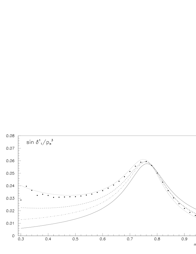
Figure 1: Function $\sin{\delta^{1}_{1}}/p_{\pi}^{3}$ deduced from $\pi^{+}\pi^{-}$ phase shifts; the function is given in units of $m_{\pi}^{-3}$. The dots correspond to the points of Ref. [9]. Full line is VMD1, dashed line is VMD2, dotted line is HLS (the best description of expected phase) and dashed–dotted is WCCWZ.

6 Summary and Conclusions

We have studied a variety of vector meson dominance models in both non–unitarised and unitarised forms. They depend on a few parameters (mass of the $\rho$ meson, its coupling constants to $\pi\pi$ and $e^{+}e^{-}$, the shape parameter $\lambda$ and the Orsay phase needed in order to describe the $\rho-\omega$ mixing). We have fitted these to both $e^{+}e^{-}\rightarrow\pi^{+}\pi^{-}$ and $e^{+}e^{-}\rightarrow\mu^{+}\mu^{-}$. In order to study the behaviour of each solution, we have studied how they match the $\pi\pi$ phase shift obtained under general model independent assumptions from threshold up to 1 GeV. We have also examined [2] the value they provide for threshold parameters ($F_{\pi}$ at threshold and the scattering length $a^{1}_{1}$), which can be estimated accurately from ChPT.

This represents the largest set of independent data and cross–checks done so far. It happens that, of the models considered, only the unitarised HLS model is able to account for all examined effects. We also find that the standard value $\lambda=1$, corresponding to a point-like $\rho\pi\pi$ coupling, is well accepted by the data for $\rho$ parametrisation.

Unlike the standard formulation of VMD, fits with this model return a significant non–resonant contribution to the electromagnetic pion form factor. This was found to have a value $\simeq-e/6$. This term is governed by a small universality violation which changes the HLS parameter $a$ from 2 to 2.4. All other models considered, even if they are able to describe $e^{+}e^{-}$ annihilations quite well, are unable to account satisfactorily for the other available information. It should be mentioned that, within the class of models considered, our results tend to favor a constant $g_{\rho\gamma}$ over a $q^{2}$ dependent one.

We conclude that, of the models considered, the HLS model with $a\simeq 2.4$ is the most favoured version for implementing the VMD ansatz. Thus, it is interesting to consider whether the success of its predictions for the magnitude and phase of $F_{\pi}(q^{2})$, could be obtained in a way which does not need the assumption that the $\rho$ is a dynamical gauge boson of a hidden local gauge symmetry. Hence, looking for other models able to describe, as successfully as the HLS model, the same large set of data is useful in order to know whether the conceptual motivation for this model should be interpreted as having any underlying significance.

References

References

- [1]
- [2] M. Benayoun, S. Eidelman, K. Maltman, H.B. O’Connell, B. Schwartz, and A.G. Williams, preprint ADP-97-14/T251, hep-ph/9707509. To appear in Zeit. Phys. C.
- [3] J.E. Augustin et al., Phys. Rev. Lett. 30 (1973) 462.
- [4] D. Benaksas et al., Phys. Lett. B39 (1972) 289.
- [5] L.M. Barkov et al., Nucl. Phys. B256 (1985) 365.
- [6] L. M. Kurdadze et al., Sov. Journ. of Nucl. Phys. 35 (1982) 201; I.B. Vasserman et al., Phys. Lett. B99 (1981) 62.
- [7] H.B. O’Connell, B.C. Pearce, A.W. Thomas and A.G. Williams, Prog. Part. Nucl. Phys. 39 (1997) 201.
- [8] W. Weise, Phys. Rep. 13 (1974) 53.
- [9] C.D. Froggatt and J.L. Petersen, Nucl. Phys. B129 (1977) 89.
- [10] M. Bando et al., Phys. Rev. Lett. 54 (1985) 1215.
- [11] S. Weinberg, Phys. Rev. 166 (1968) 1568; S. Coleman, J. Wess and B. Zumino, Phys. Rev. 177 (1969) 2239; C. Callan, S. Coleman, J. Wess and B. Zumino, ibid. 2247.
- [12] M. Birse, Zeit. Phys. A355 (1996) 231.
- [13] K. Mitchell, P. Tandy, C. Roberts and R. Cahill, Phys. Lett. B335 (1994) 282; M.R. Frank and P.C. Tandy, Phys. Rev.C49 (1994) 478; M.R. Frank, Phys. Rev. C51 (1995) 987.
- [14] H.B. O’Connell, A.G. Williams, M. Bracco and G. Krein, Phys. Lett. B370 (1996) 12.
- [15] H.B. O’Connell, B.C. Pearce, A.W. Thomas and A.G. Williams, Phys. Lett. B354 (1995) 14.
- [16] K. Maltman, H.B. O’Connell and A.G. Williams, Phys. Lett. B376 (1996) 19.
- [17] J.P. Perez-y-Jorba and F.M. Renard, Phys. Rep. 31 (1977) 1.
- [18] J.J. Sakurai, Currents and Mesons, University of Chicago Press, 1969.
- [19] F. Klingl, N. Kaiser and W. Weise, Zeit. Phys. A356 (1996) 193.
- [20] J.J. Sakurai, Ann. Phys. 11 (1960) 1.
- [21] N.M. Kroll, T.D. Lee and B. Zumino, Phys. Rev. 157 (1967) 1376.
- [22] C.J. Burden, J. Praschifka and C.D. Roberts, Phys. Rev. D46 (1992) 2695.
- [23] G. Gournaris and J. Sakurai, Phys. Rev. Lett. 21 (1968) 244.
- [24] R. Eden et al., The Analytic S Matrix, Cambridge University Press, 1966.
- [25] A. Bernicha, J. Pestieau and G. Lopez Castro, Phys. Rev. D50 (1994) 4454.
- [26] J. Pisut and M. Roos, Nucl. Phys. B6 (1968) 325.
- [27] M. Benayoun et al., Zeit. Phys. C58 (1993) 31.
- [28] M. Hashimoto, Phys. Rev. D54 (1996) 5611; Phys. Lett. B381 (1996) 465.
- [29] B.V. Geshkenbein, Zeit. Phys. C45 (1989) 351.
- [30] P.L. Chung et al., Phys. Lett. B205 (1988) 545.
- [31] M. Benayoun et al., Zeit. Phys. C65 (1995) 399.
- [32] S. Gasiorowicz, “Elementary Particle Physics”, John Wiley and Sons, New York, 1966, Chapter 26 (“Form Factors”).
- [33] S. Iwao and M. Shako, Lett. Nuovo Cim. 9 (1974) 693.
- [34] L.M. Kurdadze et al., Sov. Journ. of Nucl. Phys. 40 (1984) 286; B. Shwartz, “Investigation of the reaction at Energies up to 1400 MeV”, PhD Thesis, Novosibirsk, 1983.
- [35] R.M. Barnett et al., Review of Particle Physics, Phys. Rev. D54 (1996) 1.