1814: Search for SUSY at LHC: Precision Measurements

Abstract.

Methods to make precision measurements of SUSY masses and parameters at the CERN Large Hadron Collider are described.

1 Introduction

It is quite easy to find signals for SUSY at the LHC.[1, 2] But every SUSY event contains two missing $\tilde{\chi}_{1}^{0}$’s, so it is not possible to reconstruct masses directly. A strategy developed recently[3, 4] is to start at the bottom of the SUSY decay chain and work up it, partially reconstructing specific final states and using kinematic endpoints to determine combinations of masses. These are then fit to a model to determine the SUSY parameters. This paper is limited to discussion of this approach; search limits and inclusive measurements are discussed by Abdullin.[5]

Table 1.: Parameters for the five LHC SUGRA points.

	$m_{0}$	$m_{1/2}$	$A_{0}$	$\tan\beta$	$\mathop{\rm sgn}{\mu}$
	(GeV)	(GeV)	(GeV)
1	400	400	0	02.0	$+$
2	400	400	0	10.0	$+$
3	200	100	0	02.0	$-$
4	800	200	0	10.0	$+$
5	100	300	300	02.1	$+$

Table 2.: Representative masses for the five LHC SUGRA points in Table1.

	$M_{\tilde{g}}$	$M_{\tilde{u}_{R}}$	$M_{\tilde{W}_{1}}$	$M_{\tilde{e}_{R}}$	$M_{h}$
	(GeV)	(GeV)	(GeV)	(GeV)	(GeV)
1	1004	925	325	430	111
2	1008	933	321	431	125
3	0298	313	096	207	068
4	0582	910	147	805	117
5	0767	664	232	157	104

The LHCC (LHC Program Committee) selected five points in the minimal SUGRA model[2] for detailed study. The parameters of this model are $m_{0}$, the common scalar mass; $m_{1/2}$, the common gaugino mass; $A_{0}$, the common trilinear coupling; $\tan\beta=v_{2}/v_{1}$, the ratio of Higgs vacuum expectation values; and $\mathop{\rm sgn}\mu$, the sign of the Higgsino mass. These parameters are listed in Table1, and representative masses are listed in Table2. Point3 is the “comparison” point; LEP would have already found the light Higgs at this point. Point5 is constructed to give the right cold dark matter. Points1 and 2 have heavy masses, while Point4 has heavy squarks.

2 Specific Final States

This section describes only a few of the final states that have been studied. For all of these studies, signal and background events were generated using ISAJET[6] or PYTHIA[7], the response of the detector was simulated, and an analysis was done to select the signal from the background.

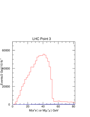
Fig. 1.: Dilepton mass distribution at Point3 and Standard Model background (shaded).[4]

$M({\tilde{\chi}}_{2}^{0})-M(\tilde{\chi}_{1}^{0})$: The prototype of precision measurements[3] is based on the decay ${\tilde{\chi}}_{2}^{0}\to\tilde{\chi}_{1}^{0}\ell^{+}\ell^{-}$ at Point3. Point3 has unusual branching ratios:

$$B({\tilde{g}}\to{\tilde{b}}_{1}\bar{b}+{\rm h.c.}) = 89\%$$

$$B({\tilde{b}}_{1}\to{\tilde{\chi}}_{2}^{0}b) = 86\%$$

$$B({\tilde{\chi}}_{2}^{0}\to\tilde{\chi}_{1}^{0}\ell^{+}\ell^{-}) = 2\times 17\%$$

Events were selected with an $\ell^{+}\ell^{-}$ pair with $p_{T,\ell}>10\,{\rm GeV}$ and $\eta<2.5$ and at least two jets tagged as $b$’s with $p_{T}>15\,{\rm GeV}$ and $\eta<2$. Efficiencies of 60% for tagging $b$’s and 90% for lepton identification were included. No $\hbox to0.0pt{\hbox to7.95831pt{\hfil/\hfil}\hss}E_{T}$ cut was used. The resulting dilepton mass distribution, Figure1, has a spectacular edge at the $M({\tilde{\chi}}_{2}^{0})-M(\tilde{\chi}_{1}^{0})$ endpoint with almost no Standard Model background. Determining the position of the edge is much easier than measuring $M_{W}$ at the Tevatron, and the statistics are huge. The estimated error for $10\,{\rm fb}^{-1}$ is $\mathchar 257\relax(M({\tilde{\chi}}_{2}^{0})-M(\tilde{\chi}_{1}^{0}))=50\,{\rm MeV}$.

The low masses and unusual branching ratios make Point3 particularly easy. But there is a similar edge at Point4 plus a $Z$ peak coming from decays of the heavier gauginos, as can be seen in Figure2.[8] In this case the estimated error is $\mathchar 257\relax\left(M({\tilde{\chi}}_{2}^{0})-M({\tilde{\chi}}_{1}^{0})\right)=\pm 1\,{\rm GeV}$. A scan of the SUGRA parameter space[10] finds an observable signal for $m_{1/2}\mathrel{\hbox to0.0pt{\raise 2.20013pt\hbox{$<$}\hss}{\lower 2.20013pt\hbox{$\sim$}}}200\,{\rm GeV}$ and for a region of small $m_{0}$ in which the sleptons are light.

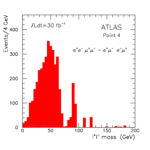
Fig. 2.: Dilepton mass distribution for Point4.[8]

${\tilde{g}}$ and ${\tilde{b}}_{1}$: The next step at Point3 is to combine an $\ell^{+}\ell^{-}$ pair near edge with jets. Events are selected as before. If the $\ell^{+}\ell^{-}$ pair has a mass near the endpoint, then the $\tilde{\chi}_{1}^{0}$ must be soft in ${\tilde{\chi}}_{2}^{0}$ rest frame, so

$$\mathchoice{\mbox{\boldmath$\bf\displaystyle p$}}{\mbox{\boldmath$\bf\textstyle p$}}{\mbox{\boldmath$\bf\scriptstyle p$}}{\mbox{\boldmath$\bf\scriptscriptstyle p$}}({\tilde{\chi}}_{2}^{0})\approx\left(1+{M(\tilde{\chi}_{1}^{0})\over M(\ell\ell)}\right)\mathchoice{\mbox{\boldmath$\bf\displaystyle p$}}{\mbox{\boldmath$\bf\textstyle p$}}{\mbox{\boldmath$\bf\scriptstyle p$}}{\mbox{\boldmath$\bf\scriptscriptstyle p$}}(\ell\ell)$$

where $M(\tilde{\chi}_{1}^{0})$ must be determined. Lepton pairs were selected with masses within $10\,{\rm GeV}$ of the endpoint and were combined with one $b$ to make $M({\tilde{b}}_{1})$ and then with a second $b$ to make $M({\tilde{g}})$. Figure3 shows a scatter plot of all combinations. Since the $\bar{b}$ jet from ${\tilde{g}}\to{\tilde{b}}\bar{b}$ is soft, there is good resolution on the $M({\tilde{g}})-M({\tilde{b}}_{1})$ mass difference — c.f. $D^{*}\to D\pi$. Varying the assumed $\tilde{\chi}_{1}^{0}$ mass gives $\mathchar 257\relax M({\tilde{b}}_{1})=\pm 1.5\mathchar 257\relax M(\tilde{\chi}_{1}^{0})\pm 3\,{\rm GeV}$ and $\mathchar 257\relax(M({\tilde{g}})-M({\tilde{b}}_{1}))=\pm 2\,{\rm GeV}$.

Fig. 3.: Scatter plot of $M({\tilde{g}})-M({\tilde{b}})$ vs. $M({\tilde{b}})$. [4]

$h\to b\bar{b}$: For Point5, ${\tilde{\chi}}_{2}^{0}\to\tilde{\chi}_{1}^{0}h$ is kinematically allowed. Events are selected with at least four jets with $p_{T}>50\,{\rm GeV}$, $p_{T,1}>100\,{\rm GeV}$, transverse sphericity $S_{T}>0.2$, $M_{\rm eff}=\hbox to0.0pt{\hbox to7.95831pt{\hfil/\hfil}\hss}E_{T}+\sum_{i=1}^{4}\,p_{T,i}>800\,{\rm GeV}$, and $\hbox to0.0pt{\hbox to7.95831pt{\hfil/\hfil}\hss}E_{T}>\max(100\,{\rm GeV},0.2M_{\rm eff})$. Then $M_{bb}$ is plotted for jets tagged as $b$’s with $p_{T,b}>25\,{\rm GeV}$ and $\eta_{b}<2$. There is a clear peak with a substantial SUSY background and small Standard Model background.

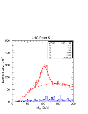
Fig. 4.: $M(bb)$ at Point5 and Standard Model background (shaded).[4]

The two jets from $h\to b\bar{b}$ can be combined with one of the two hardest jets in the event to determine the squark mass: the smaller of the two $b\bar{b}q$ masses must be less than a function of the squark mass and the other masses in the decay $\tilde{q}\to{\tilde{\chi}}_{2}^{0}q\to\tilde{\chi}_{1}^{0}hq$.

$\ell^{+}\ell^{-}$ Again: For Point5 after standard cuts one finds an edge in Figure5[9] for $>M_{Z}$. Since the two-body decay ${\tilde{\chi}}_{2}^{0}\to\tilde{\chi}_{1}^{0}h$ has been reconstructed at this point, this edge cannot come from the three-body decay ${\tilde{\chi}}_{2}^{0}\to\tilde{\chi}_{1}^{0}\ell^{+}\ell^{-}$, since the phase space is much smaller. It must come instead from ${\tilde{\chi}}_{2}^{0}\to{\tilde{\ell}}^{\pm}\ell^{\mp}\to\tilde{\chi}_{1}^{0}\ell^{\pm}\ell^{\mp}$. Thus the edge determines

$$M_{{\tilde{\chi}}_{2}^{0}}\sqrt{1-{M_{\tilde{\ell}}^{2}\over M_{\tilde{\chi}_{2}^{0}}^{2}}}\sqrt{1-{M_{\tilde{\chi}_{1}^{0}}^{2}\over M_{\tilde{\ell}}^{2}}}$$

with an error of $\pm 1\,{\rm GeV}$.

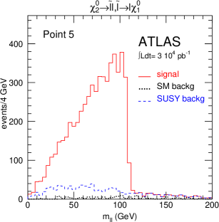
Fig. 5.: $\ell^{+}\ell^{-}$ mass distribution for Point5.[9]

It is possible to have both ${\tilde{\chi}}_{2}^{0}\to{\tilde{\ell}}_{R}\ell$ and ${\tilde{\chi}}_{2}^{0}\to\tilde{\chi}_{1}^{0}\ell\ell$ edges for some choices of the SUGRA parameters. An example is shown in Figure6.[10]

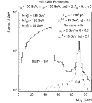
Fig. 6.: SUGRA $\ell^{+}\ell^{-}$ distribution showing edges from both ${\tilde{\chi}}_{2}^{0}\to{\tilde{\ell}}\ell$ and direct ${\tilde{\chi}}_{2}^{0}\to\tilde{\chi}_{1}^{0}\ell\ell$ decays.[10]

It should in principle be possible to extract the ${\tilde{\chi}}_{2}^{0}$, ${\tilde{\ell}}$, and $\tilde{\chi}_{1}^{0}$ masses from a fit to all the dilepton data. This has not been studied, but as a first step the distribution for the ratio $p_{T,2}/p_{T,1}$ of lepton $p_{T}$’s has been examined for $m_{0}=100,120\,{\rm GeV}$. This distribution is clearly exhibits sensitivity to the slepton mass. The same distribution can also be used to distinguish two-body and three-body decays.

$M({\tilde{g}})-M({\tilde{\chi}}_{2}^{0}),M({\tilde{\chi}}_{1}^{\pm})$: Gluino production dominates at Point4. Previously, an $\ell^{+}\ell^{-}$ edge was found at this point, determining $M({\tilde{\chi}}_{2}^{0})-M(\tilde{\chi}_{1}^{0})$. The strategy for this analysis is to select

$${\tilde{g}}+{\tilde{g}}\to{\tilde{\chi}}_{2}^{0}q\bar{q}+{\tilde{\chi}}_{1}^{\pm}q\bar{q}$$

using leptonic decays to identify ${\tilde{\chi}}_{2}^{0}$ and ${\tilde{\chi}}_{1}^{\pm}$ and so to reduce the combinatorial background. Then the jet-jet mass should have a common endpoint since $M({\tilde{\chi}}_{2}^{0})\approx M({\tilde{\chi}}_{1}^{\pm})$.

The analysis[8] requires three isolated leptons with $p_{T}>20$, 10, $10\,{\rm GeV}$ and$|\eta|<2.5$, one opposite-sign, same-flavor pair with $M_{\ell\ell}<72\,{\rm GeV}$, four jets with $p_{T}>150$, 120, 70, $40\,{\rm GeV}$, $|\eta|<3.2$, and no additional jets with $p_{T}>40\,{\rm GeV}$ and $|\eta|<5$ to minimize combinatorics. There are three pairings per event. The pairing of the two highest and the two lowest $p_{T}$ jets is unlikely and is discarded. The distribution for the remaining pairings, Figure7, shows an edge at about the right endpoint.

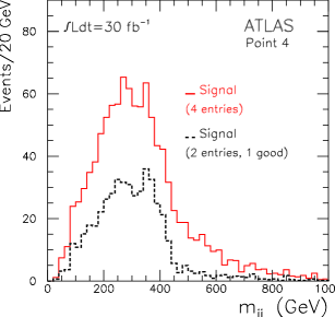
Fig. 7.: Jet-jet mass distribution for Point4 after cuts described in the text and corresponding distribution for correct pairing (dotted).[8]

3 Fitting SUGRA Parameters

Points were generated in SUGRA parameter space, and the masses were calculated and compared with the combinations of masses determined by precision measurements. FitI[4] uses a smaller set of such measurements, assumes that the Higgs mass can be related to the SUGRA parameters with an error of $3\,{\rm GeV}$, and uses an integrated luminosity of $10\,{\rm fb}^{-1}$. FitII[11] uses a larger set of precision measurements plus a few other measurements, e.g., from changing squark mass and seeing the effect on the highest $p_{T}$ jet, assumes a negligible theoretical error on the Higgs mass, and uses an integrated luminosity of $300\,{\rm fb}^{-1}$.

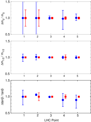
Fig. 8.: Results for FitI (circles) and Ultimate FitII (squares).

For both fits the SUGRA parameter space was scanned to determine the 68% confidence interval for each parameter. The results are summarized in Figure8. Clearly the parameters are quite well determined. No disconnected regions of parameter space were found. In particular, $\mathop{\rm sgn}\mu$ could always be determined. The gluino and squark masses are insensitive to $m_{0}$ at Points1 and 2, so FitI gives large $m_{0}$ errors. Finally, $A_{0}$ is poorly constrained in all cases. It is possible to determine the weak scale parameters $A_{t}$ and $A_{b}$, but these are insensitive to $A_{0}$.

4 $\tau$ Modes at Large $\tan\beta$

For large $\tan\beta$ the ${\tilde{\tau}}_{1}$ can be relatively light. At the SUGRA point $m_{0}=m_{1/2}=200\,{\rm GeV}$, $A_{0}=0$, $\tan\beta=45$, $\mu<0$, the decays ${\tilde{\chi}}_{2}^{0}\to{\tilde{\tau}}_{1}^{\pm}\tau^{\mp}$ and ${\tilde{\chi}}_{1}^{\pm}\to{\tilde{\tau}}_{1}^{\pm}\nu_{\tau}$ are dominant. Discovery is still straightforward, but all the analyses discussed in Section2 do not apply. One possible approach is to select 3-prong $\tau$ decays to enhance the visible $\tau$-$\tau$ mass. This is shown in Figure9; it has a clear endpoint at $M({\tilde{\chi}}_{2}^{0})-M(\tilde{\chi}_{1}^{0})$ plus a continuum from heavier gauginos. This example shows that the five LHCC points do not exhaust the possibilities even of the minimal SUGRA model.

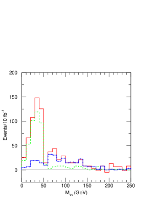
Fig. 9.: Visible $\tau$-$\tau$ mass at a large $\tan\beta$ point and contributions from ${\tilde{\chi}}_{2}^{0}$ decays (dashed) had heavy gaugino decays (dash-dotted).

5 Summary

If SUSY exists at electroweak scale, it should be easy to find signals for it at the LHC. The new result described here is that it is possible in many cases to make precision measurements of combinations of SUSY masses, and these measurements can at least in favorable cases determine the underlying SUSY parameters. While these results are quite encouraging, it seems likely that some SUSY particles — including heavy gauginos, sleptons unless ${\tilde{\chi}}_{2}^{0}\to\tilde{\ell}\ell$ or $M(\tilde{\ell})\mathrel{\hbox to0.0pt{\raise 2.20013pt\hbox{$<$}\hss}{\lower 2.20013pt\hbox{$\sim$}}}200\,{\rm GeV}$ to allow substantial Drell-Yan production, and heavy Higgs bosons — will be hard to study at the LHC, so a future lepton-lepton collider could make an important contribution.

This work was supported in part by the United States Department of Energy under Contract DE-AC02-76CH00016.

References

- [1] For general reviews of SUSY, see H.P. Nilles, Phys. Rep. 111, 1 (1984); H.E. Haber and G.L. Kane, Phys. Rep. 117, 75 (1985).
- [2] For a review of SUSY phenomenology see H.Baer, et al., FSU-HEP-950401 (1995).
- [3] A. Bartl, et al., in New Directions for High Energy Physics (Snowmass, 1996) p.693.
- [4] I. Hinchliffe, et al., Phys. Rev. D55, 5520 (1997).
- [5] S. Abdullin, these Proceedings.
- [6] H. Baer, F.E. Paige, S.D. Protopopescu, and X. Tata, Physics at Current Accelerators and Supercolliders, ed. J. Hewett, A. White and D. Zeppenfeld, (Argonne National Laboratory, 1993).
- [7] T. Sjostrand, LU-TP-95-20 (1995); S. Mrenna, Comput. Phys. Comm. 101, 232 (1997).
- [8] F. Gianotti, ATLAS Phys-No-110 (1997).
- [9] G.Polesello, L. Poggioli, E.Richter-Was, and J. Soderqvist, ATLAS Phys-No-111 (1997).
- [10] A. Kharchilava, CMS CR 1997/012 (1997).
- [11] D. Froidevaux, ATLAS Phys-No-112 (1997).