MADPH-97-1027

December, 1997

QCD CORRECTIONS TO ASSOCIATED HIGGS BOSON PRODUCTION

S. Dawson
Physics Department, Brookhaven National Laboratory,
Upton, NY 11973, USA

L. Reina
Physics Department, University of Wisconsin,
Madison, WI 53706, USA

We compute QCD corrections to the processes $e^{+}e^{-}\rightarrow t\bar{t}h^{0}$ and $pp\rightarrow t{\overline{t}}h^{0}$ by treating the Higgs boson as a parton which radiates off a heavy quark. This approximation is valid in the limits $M_{h}<<M_{t}$ and $M_{h},M_{t}<<\sqrt{s}$. The corrections increase the rate for $pp\rightarrow t{\overline{t}}h^{0}$ at the LHC by a factor of $1.2$ to $1.5$ over the lowest order rate for an intermediate mass Higgs boson, $M_{h}\!<\!180$ GeV. The QCD corrections are small for $e^{+}e^{-}\rightarrow t\bar{t}h^{0}$ at $\sqrt{s}\!=\!1$ TeV.

1 Introduction

The search for the Higgs boson is one of the most important objectives of present and future colliders. A Higgs boson or some object like it is needed in order to give the $W^{\pm}$ and $Z$ gauge bosons their observed masses and to cancel the divergences which arise when radiative corrections to electroweak observables are computed. However, we have few clues as to the expected mass of the Higgs boson, which ${\it a~{}priori}$ is a free parameter of the theory. Direct experimental searches for the Standard Model Higgs boson at LEP and LEPII yield the limit, [1]

$$M_{h}>77.5\,\,\mbox{GeV}\,\,\,\,,$$ (1)

with no room for a very light Higgs boson. LEPII will eventually extend this limit to around $M_{h}>95$ GeV. Above the LEPII limit and below the $2Z$ threshold is termed the intermediate mass region and is the most difficult Higgs mass region to probe experimentally.

In the intermediate mass region, the Higgs boson decays predominantly to $b{\overline{b}}$ pairs. Since there is an overwhelming QCD background, it appears hopeless to discover the Higgs boson through the $b{\overline{b}}$ channel alone. The associated production of the Higgs boson could offer a tag through the leptonic decay of the associated $W$ boson or top quark,[2]

$$pp \rightarrow Wh^{0}$$

$$pp \rightarrow t{\overline{t}}h^{0}\,\,\,\,.$$ (2)

Both of these production mechanisms produce a relatively small number of events, making it important to have reliable predictions for the rates.

The QCD radiative corrections to the process $pp\rightarrow Wh^{0}$ have been computed and increase the rate significantly, ($\sim 30-40\%$ at the LHC) [3, 4]. The QCD radiative corrections to the processes $e^{+}e^{-}\rightarrow t\bar{t}h^{0}$ and $pp\rightarrow t{\overline{t}}h^{0}$ do not yet exist and are the subject of this paper.

There is considerable expertise available concerning QCD corrections to Higgs production. The radiative corrections of ${\cal O}(\alpha_{s}^{3})$ to $gg\rightarrow h^{0}$ involve two-loop diagrams and have been calculated with no approximations [5]. They have also been computed in the limit in which $M_{h}/M_{t}\rightarrow 0$, where an effective Lagrangian can be used and the problem reduces to a one-loop calculation [6]. In the intermediate mass region, one expects this to be a reasonable approximation. The QCD corrections to the process $gg\rightarrow h^{0}$ can be conveniently described in terms of a $K$ factor,

$$K(\mu)_{pp\rightarrow h}\equiv{\sigma(pp\rightarrow h^{0}X)^{NLO}\over\sigma(pp\rightarrow h^{0})^{LO}}\,\,\,\,,$$ (3)

where $\mu$ is an arbitrary renormalization scale, which we take to be $\mu=M_{h}$. Fig. 1 shows the $K$ factor at the LHC computed exactly and in the $M_{h}/M_{t}\rightarrow 0$ limit. The important point is that the $M_{h}/M_{t}\rightarrow 0$ limit is extremely accurate and reproduces the exact result for the $K$ factor to within $10\%$ for all $M_{h}<1$ TeV,[4] although the small $M_{h}/M_{t}$ limit does not accurately give the total cross section for $M_{h}>M_{t}$. The reason the $K$ factor for this process is so accurately computed in the small $M_{h}/M_{t}$ limit is that a significant portion of the $K$ factor comes from a constant rescaling of the lowest order result, along with a universal contribution from the soft and collinear gluon radiation which is independent of masses [5, 6],

$$K(\mu)_{pp\rightarrow h}\sim 1+{\alpha_{s}(\mu)\over\pi}\biggl{(}\pi^{2}+{11\over 2}+....\biggr{)}\quad.$$ (4)

Hence an accurate prediction for the rate to ${\cal O}(\alpha_{s}^{3})$ can be obtained by calculating the $K$ factor in the large $M_{t}$ limit and multiplying this by the lowest order rate computed using the full mass dependence.

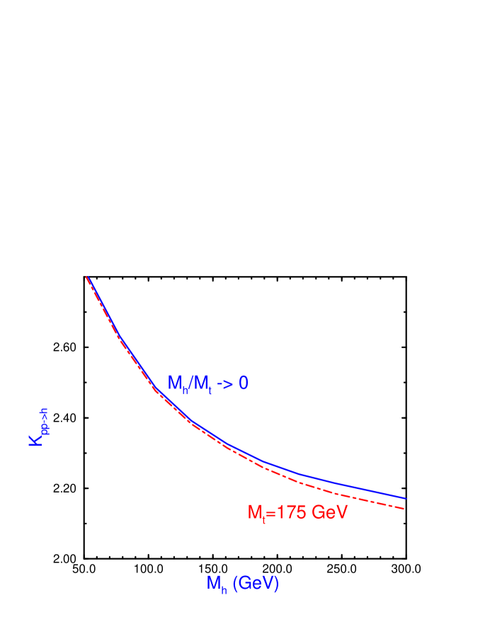
Figure 1: Ratio of the radiatively corrected cross section to the lowest order result for $pp\rightarrow h^{0}$ at the LHC, $\sqrt{s}=14$ TeV, with $\mu=M_{h}$. This figure uses the $2-$loop value of $\alpha_{s}(\mu)$ for both the lowest order and the NLO predictions.

Along this line, we compute the QCD corrections to the processes $e^{+}e^{-}\rightarrow t\bar{t}h^{0}$ and $pp\rightarrow t{\overline{t}}h^{0}$ in the $M_{h}/M_{t}\rightarrow 0$ and high energy limits, which we expect to be reasonably accurate from our experience with the $gg\rightarrow h^{0}$ process. In these limits the Higgs boson can be treated as a parton bremsstrahlung off a heavy quark. Section 2 computes the distribution of Higgs bosons in a heavy quark, $f_{t\rightarrow h}$, to leading order in ${M_{h}\over M_{t}}$, ${M_{t}\over\sqrt{s}}$, ${M_{h}\over\sqrt{s}}$ and to ${\cal O}(\alpha_{s})$ in the QCD coupling. In Section 3, we use the results of Section 2 to compute the QCD corrections to the process $e^{+}e^{-}\rightarrow t{\overline{t}}h^{0}$. We then combine the ${\cal O}({\alpha_{s}^{3}})$ corrections to $pp\rightarrow t{\overline{t}}$ [7, 8] with the ${\cal O}(\alpha_{s})$ corrections to $f_{t\rightarrow h}$ to compute the $K$ factor for $pp\rightarrow t{\overline{t}}h^{0}$ in the high energy and large $M_{t}$ limits. Just as is the case for the $gg\rightarrow h^{0}$ process, this $K$ factor can be combined with the lowest order result computed with the full mass dependences to obtain an accurate estimate of the radiatively corrected cross section. Section 4 contains some conclusions.

2 Higgs Boson Distribution Function: The Effective Higgs Approximation

2.1 Lowest Order

For a Higgs boson which has a mass much lighter than all of the relevant energy scales in a given process, $M_{h}<<M_{t}$, the Higgs boson can be treated as a parton which radiates off of the top quark. This approach was first proposed by Ellis, Gaillard, and Nanopoulos [9], and we will refer to it as to the Effective Higgs Approximation (EHA). The process $q{\overline{q}}(gg)\rightarrow t{\overline{t}}h^{0}$ can be thought of in this approximation as $q{\overline{q}}(gg)\rightarrow t{\overline{t}}$, followed by the radiation of the Higgs boson from the final state heavy quark line. This procedure is guaranteed to correctly reproduce the collinear divergences associated with the emission of a massless Higgs boson. We expect that treating the Higgs boson as a massless parton should be a good approximation for the purpose of computing radiative corrections and the $K$ factor.

The distribution function, $f_{t\rightarrow h}$, of a Higgs boson in a heavy quark, $t$, can be found from the diagram of Fig. 2 using techniques which were originally derived to find the distribution of photons in an electron [10]. This approach has also been successfully used to compute the distribution of $W$ bosons in a light quark [11].

Figure 2: The scattering process $te^{-}\rightarrow tX$ can be used to extract the Higgs boson structure function $f_{t\rightarrow h}(x_{h})$, assuming that the amplitude is dominated by the t-channel Higgs pole.

The spin- and color-averaged cross section for the scattering process $te\rightarrow tX$ through $t-$channel Higgs ($h^{0}$) exchange is,

$$\sigma(te\rightarrow tX) = {1\over 48EE_{e}}{1\over\mid{\vec{v}}_{t}-{\vec{v}}_{e}\mid}\int{{d^{3}{\vec{p}}^{~{}\prime}}\over(2\pi)^{3}}{1\over 2E^{\prime}}(2\pi)^{4}\delta^{(4)}(k+p_{e}-P_{X})$$ (5)

$$\qquad\qquad\cdot\mid{\cal A}(te\rightarrow tX)\mid^{2}d\Gamma_{X}\,\,\,\,,$$

where the kinematics are given in Fig. 2, ${\vec{v}}_{t}$ and ${\vec{v}}_{e}$ are the velocities of the incoming particles, and $d\Gamma_{X}$ is the Lorentz invariant phase space of the final state $X$. We factorize the amplitude as

$$\mid{\cal A}(te\rightarrow tX)\mid^{2}=\mid{\cal A}(eh^{0}\rightarrow X)\mid^{2}\biggl{(}{1\over k^{2}-M_{h}^{2}}\biggr{)}^{2}\mid{\cal A}(t\rightarrow th^{0})\mid^{2}.$$ (6)

This factorization is the crucial step in defining the Higgs distribution function and assumes that the dominant contribution comes from an on-shell Higgs boson.

We define the energy carried by the Higgs boson to be

$$E_{h}\equiv x_{h}E\,\,\,\,,$$ (7)

and neglect all masses, except when they lead to a logarithmic singularity. Using

$$\sigma(eh^{0}\rightarrow X)={1\over 8E_{h}E_{e}}d\Gamma_{X}(2\pi)^{4}\delta^{4}(k+p_{e}-P_{X})\mid{\cal A}(eh^{0}\rightarrow X)\mid^{2}\quad,$$ (8)

and $d^{3}{\vec{p}}^{~{}\prime}=(1-x_{h})^{2}E^{3}dx_{h}d\Omega^{\prime}$ we find

$$\sigma(te\rightarrow tX)={E^{2}\over 96\pi^{3}}\int dx_{h}~{}x_{h}(1-x_{h})\int{d\Omega^{\prime}\over k^{4}}\mid{\cal A}(t\rightarrow th^{0})\mid^{2}\sigma(eh^{0}\rightarrow X)\quad.$$ (9)

We now define the Higgs boson structure function by the relation,

$$\sigma(te\rightarrow tX)\equiv\int f_{t\rightarrow h}(x_{h})\sigma(eh^{0}\rightarrow X)dx_{h}\quad.$$ (10)

This is a Lorentz invariant definition which can be used beyond the leading order. We use the notation $f^{0}_{t\rightarrow h}(x_{h})$ to denote the lowest order result,

$$f^{0}_{t\rightarrow h}(x_{h})={E^{2}\over 96\pi^{3}}x_{h}(1-x_{h})\int{d\Omega^{\prime}\over k^{4}}\mid{\cal A}(t\rightarrow th^{0})\mid^{2},$$ (11)

where ${\cal A}(t\rightarrow th^{0})\equiv-ig_{t}\delta_{ij}\bar{u}(p^{\prime})u(p)$.

We now consider a Higgs boson which couples to heavy quarks with the Yukawa interaction,

$${\cal L}=-g_{t}{\overline{t}}th^{0}\,\,\,.$$ (12)

In the Standard Model, $g_{t}={M_{t}\over v}$, with $v=246$ GeV. Our calculation is, however, valid in any model where $M_{h}<<M_{t}$, such as a SUSY model.

Performing the integral of Eq. (11), we obtain our primary result,

$$f^{0}_{t\rightarrow h}(x_{h}) = {g_{t}^{2}\over 16\pi^{2}}\biggl{\{}{4(1-x_{h})\over x_{h}}+x_{h}\log\biggl{(}{4E^{2}(1-x_{h})^{2}\over M_{t}^{2}x_{h}^{2}}\biggr{)}\biggr{\}}$$ (13)

$$+{\cal O}\biggl{(}{M_{t}\over E},{M_{h}\over E},{M_{h}\over M_{t}}\biggr{)}\,\,\,\,.$$

The dominant numerical contribution comes from the $(1-x_{h})/x_{h}$ term, i.e. from the infrared part of the Higgs distribution function. In fact, we can also reproduce the first term in Eq. (13) if we calculate, in the eikonal approximation, the bremsstrahlung of a soft Higgs from the final state of the $e^{+}e^{-}\rightarrow t\bar{t}$ process. This provides us with an independent check of the leading behavior of the Higgs structure function we are going to use in the following.

It is instructive to compute the neglected mass dependent terms using a different approach. The cross section for $q{\overline{q}}\rightarrow t{\overline{t}}h^{0}$ has been computed many years ago [12],

$${d\sigma(q{\overline{q}}\rightarrow t{\overline{t}}h^{0})\over dx_{h}} = {\alpha_{s}^{2}g_{t}^{2}\over 27\pi s}\biggl{\{}\biggl{[}x_{h}+2\biggl{(}{4M_{t}^{2}-M_{h}^{2}\over s}\biggr{)}$$ (14)

$$+{2\over x_{h}}{(4M_{t}^{2}-M_{h}^{2})(2M_{t}^{2}-M_{h}^{2})\over s^{2}}+{8M_{t}^{2}\over sx_{h}}\biggl{]}\log\biggl{(}{x_{h}+{\hat{\beta}}\over x_{h}-{\hat{\beta}}}\biggr{)}$$

$$+{4{\hat{\beta}}\over x_{h}^{2}-{\hat{\beta}}^{2}}\biggl{(}1+{2M_{t}^{2}\over s}\biggr{)}\biggr{(}{4M_{t}^{2}-M_{h}^{2}\over s}\biggr{)}\biggr{\}}\,\,\,\,,$$

where $x_{h}=2E_{h}/\sqrt{s}$ is the exact equivalent of the quantity defined in Eq. (7) and varies in the range between

$$x_{h}^{min}=\frac{2M_{h}}{\sqrt{s}}\,\,\,\,\,\,\,\,\,\mbox{and}\,\,\,\,\,\,\,\,x_{h}^{max}=1-\frac{4M_{t}^{2}}{s}+\frac{M_{h}^{2}}{s}\,\,\,\,\,,$$ (15)

while $\hat{\beta}$ is defined to be

$$\hat{\beta}=\left[\frac{(x_{h}^{2}-(x_{h}^{min})^{2})(x_{h}^{max}-x_{h})}{(x_{h}^{max}-x_{h}+4M_{t}^{2}/s)}\right]^{1/2}\,\,\,\,.$$ (16)

We can define the distribution of Higgs bosons in a heavy quark by the relation,

$$\sigma(q{\overline{q}}\rightarrow t{\overline{t}}h^{0})=2\int dx_{h}\sigma(q{\overline{q}}\rightarrow t{\overline{t}}){\hat{f}}_{t\rightarrow h}(x_{h})\,\,\,\,,$$ (17)

where the factor of $2$ reflects the fact that the Higgs boson can radiate from either quark. Using Eq. (17) we find an alternate definition of the Higgs distribution function,

$${\hat{f}}_{t\rightarrow h}(x_{h})=\biggl{[}{1\over 2\sigma(q{\overline{q}}\rightarrow t{\overline{t}})}\biggr{]}{d\sigma(q{\overline{q}}\rightarrow t{\overline{t}}h)\over dx_{h}}\,\,\,\,.$$ (18)

Taking the limit $s>>M_{t}^{2}>>M_{h}^{2}$ of Eq. (14), we find

$${\hat{f}}_{t\rightarrow h}(x_{h})={g_{t}^{2}\over 16\pi^{2}}\biggl{\{}x_{h}\log\biggl{(}{s(1-x_{h})\over M_{t}^{2}}\biggr{)}+4\biggl{(}{1-x_{h}\over x_{h}}\biggr{)}\biggr{\}}\,\,\,\,.$$ (19)

Except for the argument of the logarithm, this agrees with Eq. (13). It is easy to convince ourselves that this discrepancy can only introduce a difference of the same order of magnitude as the effects we are neglecting and is therefore irrelevant in our approximation. We have explicitely checked that the use of $f_{t\rightarrow h}(x_{h})$ in the form of Eq. (13) or of Eq. (19) is numerically irrelevant for an intermediate mass Higgs boson and parton sub-energies above around $1$ TeV.

2.2 QCD Corrections

The utility of the results of the previous section is that it is straightforward to compute the ${\cal O}(\alpha_{s})$ corrections to $f_{t\rightarrow h}$. The discussion here parallels that of Ref. [13].

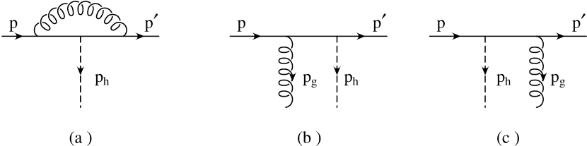
Figure 3: Virtual (a) and real (b,c) QCD corrections to be computed in order to obtain the $O(\alpha_{s})$ corrections to the structure function $f_{t\rightarrow h}(x_{h})$ in the EHA.

2.2.1 Virtual Corrections

The virtual corrections include contributions from the vertex renormalization of Fig. 3a, from the top quark wavefunction renormalization, and from the top quark mass renormalization. The virtual correction from Fig. 3a is given by,

$${\cal A}_{V} = {\cal A}^{0}(t\rightarrow th^{0})\frac{\alpha_{s}}{4\pi}C_{F}\left[\left(\frac{4\pi\mu^{2}}{M_{t}^{2}}\right)^{\epsilon}4(1+2\epsilon)\Gamma_{UV}(\epsilon)-6\,\right.$$ (20)

$$+\left.\left(\frac{4\pi\mu^{2}}{M_{t}^{2}}\right)^{\epsilon}(2-r_{h})\left(\Gamma_{IR}(\epsilon)+\frac{r_{h}}{6}(1-\epsilon)\Gamma_{IR}(\epsilon)+O(r_{h}^{2})\right)\right],$$

where we define $r_{h}=M_{h}^{2}/M_{t}^{2}$ and $C_{F}={4\over 3}$. ${\cal A}^{0}(t\rightarrow th^{0})$ denotes the tree level amplitude for $t\rightarrow th^{0}$, and can be directly read from Eq. (12). We have explicitely separated the infrared ($\epsilon_{IR}$) and ultraviolet ($\epsilon_{UV}$) divergences and we have defined

$$\Gamma(\epsilon)=\frac{1}{\epsilon}-\gamma_{E}\equiv\frac{1}{\epsilon^{\prime}}\,\,\,.$$ (21)

The wave function renormalization ($Z_{2}$) contributes to the virtual amplitude,

$$Z_{2}{\cal A}^{0}(t\rightarrow th^{0}) = -{\cal A}^{0}(t\rightarrow th^{0})\frac{\alpha_{s}}{4\pi}\left(\frac{4\pi\mu^{2}}{M_{t}^{2}}\right)^{\epsilon}C_{F}\biggl{[}(1+2\epsilon)\Gamma_{UV}(\epsilon)+2(1+\epsilon)\Gamma_{IR}(\epsilon)\biggr{]}$$ (22)

$$= -{\cal A}^{0}(t\rightarrow th^{0})\frac{\alpha_{s}}{4\pi}\left(\frac{4\pi\mu^{2}}{M_{t}^{2}}\right)^{\epsilon}C_{F}\left(\frac{1}{\epsilon_{UV}^{\prime}}+\frac{2}{\epsilon_{IR}^{\prime}}+4\right).$$

The sum of (22) and (20) has both an UV pole and an IR pole. The UV pole in fact is cancelled by the renormalization of the mass term in the Higgs-fermion coupling ($g_{t}=M_{t}/v$), while the IR pole will be cancelled by the soft gluon bremsstrahlung contribution (see Fig. 3b and 3c). To complete the calculation of the virtual part, we add to (22) and (20) the mass renormalization, i.e.

$$\delta{M_{t}}=-M_{t}\frac{\alpha_{s}}{4\pi}C_{F}\left(\frac{4\pi\mu^{2}}{M_{t}^{2}}\right)^{\epsilon}\Gamma_{UV}(\epsilon)(3+4\epsilon)\,\,\,\,,$$ (23)

and we obtain,

$${\cal A}_{virt}\equiv{\cal A}^{0}(t\rightarrow th^{0})\frac{\alpha_{s}}{4\pi}C_{F}\left[-\frac{2}{3}r_{h}\Gamma_{IR}(\epsilon)\left(\frac{4\pi\mu^{2}}{M_{t}^{2}}\right)^{\epsilon}-6-\frac{1}{3}r_{h}+O(r_{h}^{2})\right].$$ (24)

Therefore, the virtual processes contribute to the QCD corrected Higgs distribution function,

$$f_{t\rightarrow h}^{virt}(x_{h})=f^{0}_{t\rightarrow h}(x_{h})\left\{1+\frac{\alpha_{s}}{2\pi}C_{F}\left[-\frac{2}{3}r_{h}\Gamma_{IR}(\epsilon)\left(\frac{4\pi\mu^{2}}{M_{t}^{2}}\right)^{\epsilon}-6-\frac{1}{3}r_{h}+O(r_{h}^{2})\right]\right\}\,\,\,\,.$$ (25)

In the limit $r_{h}\rightarrow 0$ we have

$$f_{t\rightarrow h}^{virt}(x_{h})\rightarrow f^{0}_{t\rightarrow h}(x_{h})\left\{1-\frac{3\alpha_{s}}{\pi}C_{F}\right\}.$$ (26)

2.2.2 Real Corrections

The gluon bremsstrahlung diagrams are shown in Fig. 3b and 3c. In the soft gluon limit, the amplitude is given by,

$${\cal A}(t\rightarrow th^{0}g)^{soft}=g_{s}T^{a}_{ij}{\cal A}^{0}(t\rightarrow th^{0})\biggl{(}{p^{\prime}\cdot\epsilon_{g}\over p^{\prime}\cdot p_{g}}-{p\cdot\epsilon_{g}\over p\cdot p_{g}}\biggr{)}\,\,\,\,.$$ (27)

The contribution to the Higgs distribution function is found by integrating over the gluon phase space,

$$(PS)_{g}=\int_{0}^{\delta}dE_{g}{E_{g}^{1-2\epsilon}\over(2\pi)^{3-2\epsilon}}\int_{0}^{\pi}\sin^{1-2\epsilon}\theta_{1}d\theta_{1}\int^{\pi}_{0}\sin^{-2\epsilon}\theta_{2}d\theta_{2},$$ (28)

where $E_{g}$ is the gluon energy. The integral of Eq. (28) is cut off at an arbitrary energy scale, $\delta$, and the dependence on $\delta$ must vanish when the hard gluon terms are included. Performing the integrals of Eq. (28), the soft gluon bremsstrahlung term is given by

$$f_{t\rightarrow h}^{brem}(x_{h})=f_{t\rightarrow h}^{0}(x_{h})\frac{\alpha_{s}}{2\pi}C_{F}\left\{\frac{2}{3}r_{h}\Gamma(\epsilon_{IR})\left(\frac{4\pi\mu^{2}}{\delta^{2}}\right)^{\epsilon}+\Delta+O(r_{h}^{2})\right\}\,\,\,\,,$$ (29)

In Eq. (29), $\Delta$ is the sum of all the remaining finite contributions,

$$\Delta = -\frac{2}{3}r_{h}\log(4)+\frac{1}{\beta_{p}}\log\left(\frac{1+\beta_{p}}{1-\beta_{p}}\right)+\frac{1}{\beta_{p^{\prime}}}\log\left(\frac{1+\beta_{p^{\prime}}}{1-\beta_{p^{\prime}}}\right)$$ (30)

$$-(2-r_{h})\int_{0}^{1}{du\over\beta_{v}(u)}\frac{\log\left(\frac{1+\beta_{v}(u)}{1-\beta_{v}(u)}\right)}{[1-u(1-u)r_{h}]}\,\,\,\,,$$

and we have denoted by

$$\beta_{p}=\left(1-\frac{M_{t}^{2}}{E^{2}}\right)^{1/2}\,\,\,\,\,\,\mbox{and}\,\,\,\,\,\,\beta_{p^{\prime}}=\left(1-\frac{M_{t}^{2}}{E^{\prime 2}}\right)^{1/2}$$ (31)

the velocities of the incoming ($p$) and of the outgoing ($p^{\prime}$) t-quark respectively, while

$$\beta_{v}(u)=\left(1-\frac{m_{v}(u)^{2}}{E_{v}(u)^{2}}\right)^{1/2}$$ (32)

is the $\beta$-term velocity for the $4-$vector $v\equiv up+(1-u)p^{\prime}$, which we use in the integration of the interference term between the two real emission diagrams. In the limit $r_{h}\rightarrow 0$ and $M_{t}<<E,E^{\prime}$,

$$\Delta\rightarrow\frac{1}{2}\left\{4\biggl{(}{E+E^{\prime}\over E-E^{\prime}}\biggr{)}\log\biggl{(}{E^{\prime}\over E}\biggr{)}+8\right\}\,\,\,\,.$$ (33)

We can see that in the sum of (25) and (29) the residual IR divergences cancel.

The final QCD corrected result is

$$f_{t\rightarrow h}(x_{h}) = f_{t\rightarrow h}^{0}(x_{h})\biggl{\{}1+{\alpha_{s}(\mu)\over{\pi}}C_{F}\biggl{[}-1+{2-x_{h}\over x_{h}}\log(1-x_{h})\biggr{]}\biggr{\}}+f^{hard}+{\cal O}(r_{h})$$ (34)

$$\equiv f_{t\rightarrow h}^{0}(x_{h})\biggl{\{}1+{\alpha_{s}(\mu)\over\pi}f_{t\rightarrow h}^{1}(x_{h})\biggr{\}}\,\,\,\,.$$

The hard gluon terms cannot be reproduced in this approximation and they would require the full calculation of the bremsstrahlung of a hard gluon in the final state of $e^{+}e^{-}\rightarrow t\bar{t}h^{0}$ or $pp\rightarrow t\bar{t}h^{0}$. Note that to leading order in $r_{h}$ there is no dependence on the gluon energy cut-off $\delta$ in the soft bremsstrahlung contribution of Eq. (29) and so $f^{hard}$ can contain only finite terms. In addition, there can be no $1/x_{h}$ singularities in $f^{hard}$ and so we expect this term to be small. The emission of a hard gluon should have a very distinguishable experimental signature and should not affect the study of $e^{+}e^{-}\rightarrow t\bar{t}h^{0}$ or $pp\rightarrow t\bar{t}h^{0}$. Therefore we do not include the study of hard gluon emission in this context and drop the $f^{hard}$ part of the structure function $f_{t\rightarrow h}(x_{h})$.

Figure 4 shows the lowest order and radiatively corrected results for 2 typical energy scales. It is clear that the dominant contribution is from the $(1-x_{h})/x_{h}$ term with little energy dependence and that the order ${\cal O}(\alpha_{s})$ contributions are small.

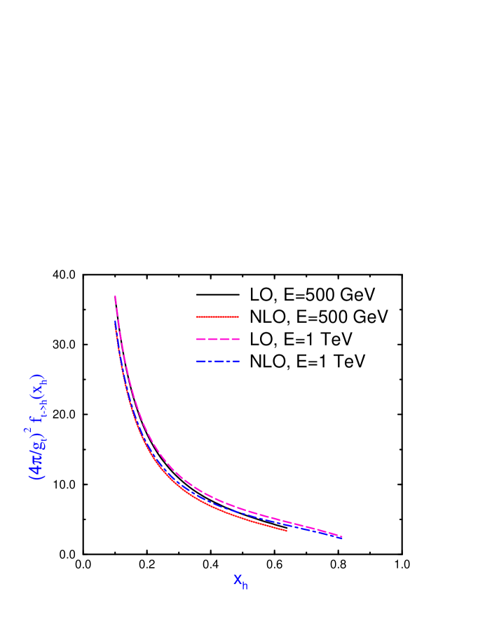
Figure 4: The Higgs distribution function $f_{t\rightarrow h}(x_{h})$ in units of $g_{t}^{2}/(4\pi)^{2}$.

3 Cross Sections

3.1 $e^{+}e^{-}\rightarrow t{\overline{t}}h^{0}$

As a first application of the formalism previously derived, we want now to estimate the impact of QCD corrections on the cross section for $e^{+}e^{-}\rightarrow t\bar{t}h^{0}$. This will require us to use the QCD corrected distribution function derived in Eq. (34) together with the NLO expression for the cross section for $e^{+}e^{-}\rightarrow t\bar{t}$.

Let us start testing the validity of the EHA approach in the absence of QCD corrections. For this purpose, we evaluate and compare the cross section for $e^{+}e^{-}\rightarrow t\bar{t}h^{0}$ in the exact theory (i.e. the Standard Model) and in the EHA, for an intermediate mass Higgs boson.

The cross section for $e^{+}e^{-}\rightarrow t\bar{t}h^{0}$ has been first calculated in [14] (photon-exchange contribution only) and then completed in [15] (both photon and $Z$-exchange contributions). To make the comparison with the formalism explained in Section 2 easier, we will write the cross section in the form

$$\sigma(e^{+}e^{-}\rightarrow t\bar{t}h^{0})=\int_{x_{h}^{min}}^{x_{h}^{max}}dx_{h}\frac{d\sigma(e^{+}e^{-}\rightarrow t\bar{t}h^{0})}{dx_{h}}\,\,\,\,,$$ (35)

where $x_{h}=2E_{h}/\sqrt{s}$ and the integration bounds have been defined in Eq. (15). The differential distribution in Eq. (35) can be written as

$$\frac{d\sigma(e^{+}e^{-}\rightarrow t\bar{t}h^{0})}{dx_{h}} = N_{c}\frac{\sigma_{0}}{(4\pi)^{2}}\left\{\left[Q_{e}^{2}Q_{t}^{2}+\frac{2Q_{e}Q_{t}V_{e}V_{t}}{1-M_{Z}^{2}/s}+\frac{(V_{e}^{2}+A_{e}^{2})(V_{t}^{2}+A_{t}^{2})}{(1-M_{Z}^{2}/s)^{2}}\right]G_{1}+\right.$$ (36)

$$\left.\frac{V_{e}^{2}+A_{e}^{2}}{(1-M_{Z}^{2}/s)^{2}}\left[A_{t}^{2}\sum_{i=2}^{6}G_{i}+V_{t}^{2}(G_{4}+G_{6})\right]+\frac{Q_{e}Q_{t}V_{e}V_{t}}{1-M_{Z}^{2}/s}G_{6}\right\}\,\,\,\,,$$

where $\sigma_{0}\!=\!4\pi\alpha_{e}^{2}/3s$, $\alpha_{e}$ is the QED fine structure constant, and $Q_{i}$, $V_{i}$ and $A_{i}$ ($i\!=\!e$, $t$) denote the electromagnetic and weak couplings of the electron and of the top quark respectively,

$$V_{i}=\frac{2I_{3L}^{i}-4Q_{i}s_{W}^{2}}{4s_{W}c_{W}}\,\,\,\,\,\,\,\,,\,\,\,\,\,\,\ A_{i}=\frac{2I_{3L}^{i}}{4s_{W}c_{W}}\,\,\,\,,$$ (37)

with $I_{3L}^{i}\!=\!\pm 1/2$ being the weak isospin of the left-handed fermions and $s_{W}^{2}\!=\!1-c_{W}^{2}=0.23$.

The coefficients $G_{1}$ and $G_{2}$ describe the radiation of the Higgs boson off the top quark (both photon and $Z$ boson exchange), while $G_{3},\ldots,G_{6}$ represent the radiation of the Higgs boson off the $Z$ boson. Explicit expressions for the coefficients $G_{1},\ldots,G_{6}$ are given in the Appendix.

As already observed in Ref. [15], the most relevant contributions are those in which the Higgs boson is emitted from a top quark leg, i.e. those proportional to $G_{1}$ and $G_{2}$ in Eq. (36). This is further confirmed when we calculate the same process in the EHA and we see that it is numerically consistent with the exact result to within a factor of $1.5-1.8$ for $50\leq M_{h}\leq 150$ GeV and $\sqrt{s}\!=\!1$ TeV (the agreement is clearly improved when we go to higher values of $\sqrt{s}$).

In fact, according to Section 2, the cross section for $e^{+}e^{-}\rightarrow t\bar{t}h^{0}$ is evaluated in the EHA as the convolution of the Higgs boson distribution function with the cross section for $e^{+}e^{-}\rightarrow t\bar{t}$, i.e.

$$\sigma(e^{+}e^{-}\rightarrow t\bar{t}h^{0})_{EHA}=2\int_{x_{h}^{min}}^{x_{h}^{max}}dx_{h}f^{0}_{t\rightarrow h}(x_{h})\sigma(e^{+}e^{-}\rightarrow t\bar{t})\,\,\,\,,$$ (38)

and therefore only the emission of a Higgs boson from a top quark is taken into account.

In the absence of QCD corrections, $f^{0}_{t\rightarrow h}(x_{h})$ is given by Eq. (13), while $\sigma(e^{+}e^{-}\rightarrow t\bar{t})$ can be easily calculated and reads [16, 17]

$$\sigma(e^{+}e^{-}\rightarrow t\bar{t})=\beta_{t}\left(1+\frac{1}{2}\mu_{t}^{2}\right)\sigma_{VV}+\beta_{t}^{3}\sigma_{AA}\,\,\,\,,$$ (39)

where $\mu_{t}\!=\!2M_{t}/\sqrt{s}$, $\beta_{t}^{2}\!=\!(1-\mu_{t}^{2})$, and $\sigma_{VV}$ and $\sigma_{AA}$ correspond respectively to the product of two vector or two axial currents (the interference between the two gives zero upon angular integration),

$$\sigma_{VV} = N_{c}\sigma_{0}\left[Q_{e}^{2}Q_{t}^{2}+2Q_{e}Q_{t}V_{e}V_{t}\frac{s}{s-M_{Z}^{2}}+V_{t}^{2}(V_{e}^{2}+A_{e}^{2})\left(\frac{s}{s-M_{Z}^{2}}\right)^{2}\right]$$

$$\sigma_{AA} = N_{c}\sigma_{0}\,A_{t}^{2}(V_{e}^{2}+A_{e}^{2})\left(\frac{s}{s-M_{Z}^{2}}\right)^{2}\,\,\,\,,$$ (40)

using the same notation we introduced before. We notice that $\sigma(e^{+}e^{-}\rightarrow t\bar{t})$ does not depend on $x_{h}$ and the associated Higgs production, in the EHA, is obtained by simply multiplying $\sigma(e^{+}e^{-}\rightarrow t\bar{t})$ by a prefactor, as can be seen from Eq. (38).

In Figure 5 we compare the exact cross section of Eq. (35) to the EHA one of Eq. (38), in terms of their ratio

$$R=\frac{\sigma(e^{+}e^{-}\rightarrow t\bar{t}h^{0})_{EHA}}{\sigma(e^{+}e^{-}\rightarrow t\bar{t}h^{0})_{EXACT}}\quad.$$ (41)

As we can see, the EHA reproduces the exact cross section to a good level of approximation and we are entitled to use it in the estimate of the impact of QCD corrections on the associated production of an intermediate mass Higgs boson in $t\bar{t}$ events.

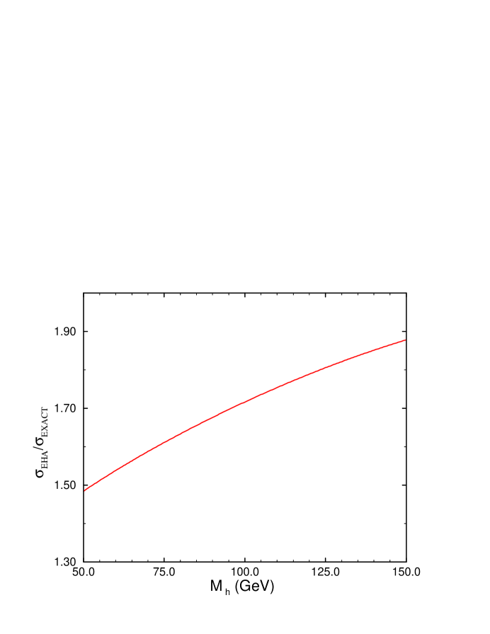
Figure 5: Ratio of the lowest order cross section computed in the EHA for $e^{+}e^{-}\rightarrow t\bar{t}h^{0}$ to the same quantity computed exactly, for intermediate mass Higgs bosons at $\sqrt{s}=1$ TeV.

Within the EHA formalism, we can parameterize the effect of QCD corrections as

$$\sigma(e^{+}e^{-}\rightarrow t\bar{t}h^{0})=2\left[\int_{x_{h}^{min}}^{x_{h}^{max}}dx_{h}f^{0}_{t\rightarrow h}(x_{h})\left(1+\frac{\alpha_{s}(\mu)}{\pi}f^{1}_{t\rightarrow h}(x_{h})\right)\right]\left(\hat{\sigma}^{0}+\frac{\alpha_{s}(\mu)}{\pi}\hat{\sigma}^{1}\right)\,\,\,\,,$$ (42)

where $f^{0}_{t\rightarrow h}$ is the Higgs boson distribution function without QCD corrections, as in Eq. (13), while the exact expression of $f^{1}_{t\rightarrow h}(x_{h})$ can be derived from Eq. (34). Moreover, we have schematically represented the QCD corrected cross section $\sigma(e^{+}e^{-}\rightarrow t\bar{t})$ in the form

$$\sigma(e^{+}e^{-}\rightarrow t\bar{t})=\hat{\sigma}_{0}+\frac{\alpha_{s}(\mu)}{\pi}\hat{\sigma}^{1}\,\,\,\,,$$ (43)

where $\hat{\sigma}_{0}$ is given in Eq. (39).

Numerical expressions for $\hat{\sigma}^{1}$ at various energies can be found in the literature [17] and we refer to these numbers in our discussion. The impact of QCD corrections on the prediction of the cross section for $e^{+}e^{-}\rightarrow t\bar{t}h^{0}$ is described by the K-factor,

$$K(\mu)_{e^{+}e^{-}\rightarrow t\bar{t}h}=\frac{\sigma(e^{+}e^{-}\rightarrow t\bar{t}h^{0})^{NLO}}{\sigma(e^{+}e^{-}\rightarrow t\bar{t}h^{0})^{LO}}\quad.$$ (44)

In the EHA, using Eq. (38) and Eq. (42), the K-factor can be written as

$$K(\mu)_{e^{+}e^{-}\rightarrow t\bar{t}h} = \frac{\left[\int_{x_{h}^{min}}^{x_{h}^{max}}dx_{h}f^{0}_{t\rightarrow h}(x_{h})\left(1+\frac{\alpha_{s}(\mu)}{\pi}f^{1}_{t\rightarrow h}(x_{h})\right)\right]\left(\hat{\sigma}^{0}+\frac{\alpha_{s}(\mu)}{\pi}\hat{\sigma}^{1}\right)}{\left[\int_{x_{h}^{min}}^{x_{h}^{max}}dx_{h}f^{0}_{t\rightarrow h}(x_{h})\right]\hat{\sigma}^{0}}$$ (45)

$$= 1+\frac{\alpha_{s}(\mu)}{\pi}\left(\frac{\hat{\sigma}^{1}}{\hat{\sigma}^{0}}+\frac{\int_{x_{h}^{min}}^{x_{h}^{max}}dx_{h}f^{0}_{t\rightarrow h}(x_{h})f^{1}_{t\rightarrow h}(x_{h})}{\int_{x_{h}^{min}}^{x_{h}^{max}}dx_{h}f^{0}_{t\rightarrow h}(x_{h})}\right)\,\,\,\,.$$

Using the results of Ref. [17], we can estimate that $\hat{\sigma}^{1}/\hat{\sigma}^{0}\!\simeq\!1.7$ at $\sqrt{s}\!=\!1$ TeV (taking $\mu=\sqrt{s}$ and $\alpha_{s}(s)\!=\!0.088$), while the second term in parenthesis is roughly $-4$ for $M_{h}<180$ GeV. Therefore $K(s)\!\simeq.94$ and the impact of QCD corrections is estimated in the EHA to be very mild for $e^{+}e^{-}$ initial states.

3.2 $pp\rightarrow t{\overline{t}}h^{0}$

The QCD corrections to the process $pp\rightarrow t{\overline{t}}h^{0}$ can be estimated using the EHA and the results of Ref. [7, 8] for the NLO corrections to $pp\rightarrow t{\overline{t}}$. The NLO cross section for $t{\overline{t}}$ production at a hadron collider can be conveniently parameterized at the parton level as,

$$\sigma(ij\rightarrow t{\overline{t}}X)={\alpha_{s}^{2}(\mu)\over M_{t}^{2}}\biggl{\{}f_{ij}^{0}({\hat{\rho}})+4\pi\alpha_{s}(\mu)\biggl{[}f_{ij}^{1}({\hat{\rho}})+{\overline{f}}_{ij}^{1}({\hat{\rho}})\log\biggl{(}{\mu^{2}\over M_{t}^{2}}\biggr{)}\biggr{]}\biggr{\}}\,\,\,\,,$$ (46)

where $ij$ corresponds to the $gg$, $q{\overline{q}}$, $qg$, and ${\overline{q}}g$ initial states and

$${\hat{\rho}}={4M_{t}^{2}\over{\hat{s}}}\,\,\,\,,$$ (47)

with ${\hat{s}}$ the parton sub-energy. Analytic results for the $f_{ij}^{0}({\hat{\rho}})$ and ${\overline{f}}_{ij}^{1}({\hat{\rho}})$ and numerical parameterizations of $f_{ij}^{1}({\hat{\rho}})$ can be found in Ref. [7].

In the EHA, the cross section for $pp\rightarrow t{\overline{t}}h^{0}$ production at lowest order is then,

$$\sigma^{0}(pp\rightarrow t\bar{t}h^{0})={2\alpha_{s}^{2}(\mu)\over M_{t}^{2}}\int dx_{1}dx_{2}\sum_{ij}F_{i}(x_{1})F_{j}(x_{2})f_{ij}^{0}({\hat{\rho}})\int dx_{h}f_{t\rightarrow h}^{0}(x_{h}),$$ (48)

where $F_{i}(x)$ are the parton distribution functions and $x_{1}$ and $x_{2}$ are the momentum fractions carried by the incoming partons. Again, the over-all factor of $2$ reflects the fact that the Higgs boson can be radiated off either top quark leg. The parton sub-energy is ${\hat{s}}=x_{1}x_{2}s$. Note that because of the dependence on ${\hat{s}}$ in $f_{t\rightarrow h}(x_{h})$, the effect of the Higgs emission is not a simple prefactor as was the case for $e^{+}e^{-}$, (although the energy dependence is very small).

At lowest order, the process $pp\rightarrow t{\overline{t}}h^{0}$ includes both the $q{\overline{q}}$ and $gg$ initial states. As was the case for $e^{+}e^{-}$, the contribution from the $q{\overline{q}}$ initial state is well approximated at lowest order in the intermediate mass Higgs region by the EHA calculation. However, the process $gg\rightarrow t{\overline{t}}h^{0}$ also contains the $t$ -channel emission of a Higgs boson which is not included in the EHA approximation and so the EHA is a much poorer approximation to the lowest order hadronic cross section than it is to the $e^{+}e^{-}$ cross section. We will therefore use the EHA only to calculate the $K$ factor. The best estimate of the rate for $pp\rightarrow t\bar{t}h^{0}$ will then be obtained by using the exact calculation for the lowest order rate and then multiplying by the $K$ factor obtained using the EHA.

The cross section to NLO can easily be found using the EHA,

$$\sigma^{1}(pp\rightarrow t{\overline{t}}h^{0}) = {2\alpha_{s}^{2}(\mu)\over M_{t}^{2}}\int dx_{1}dx_{2}\sum_{ij}F_{i}(x_{1})F_{j}(x_{2})\int dx_{h}f^{0}_{t\rightarrow h}(x_{h})\biggl{\{}f_{ij}^{0}(\hat{\rho})$$ (49)

$$+{\alpha_{s}(\mu)\over\pi}\biggl{(}f^{1}_{t\rightarrow h}(x_{h})+(4\pi^{2})\biggl{[}f_{ij}^{1}(\hat{\rho})+{\overline{f}}_{ij}^{1}(\hat{\rho})\log\biggl{(}{\mu^{2}\over M_{t}^{2}}\biggr{)}\biggl{]}\biggr{)}\biggr{\}}\,\,\,\,.$$

The $K$ factor is then given as usual by,

$$K(\mu)_{pp\rightarrow t{\overline{t}}h}\equiv{\sigma^{1}(pp\rightarrow t{\overline{t}}h^{0})\over\sigma^{0}(pp\rightarrow t{\overline{t}}h^{0})}\,\,\,\,.$$ (50)

In Fig. 6, we show the $K$ factor using structure functions derived by Morfin and Tung.[18] It is clear from this figure that using the lowest order cross section with the $2-$loop evolution of $\alpha_{s}(\mu)$ overestimates the size of the corrections. (This is also true for the $pp\rightarrow h^{0}$ process.[4]) The $K$ factor varies between around $1.2$ and $1.5$ for the intermediate mass Higgs boson. Since the dominant production mechanism is gluon fusion, the exact value of the $K$ factor is sensitive to the choice of structure functions. We have found that changing the set of structure functions induces a $10-20~{}\%$ uncertainty in the $K$ factor shown in Fig. 6.

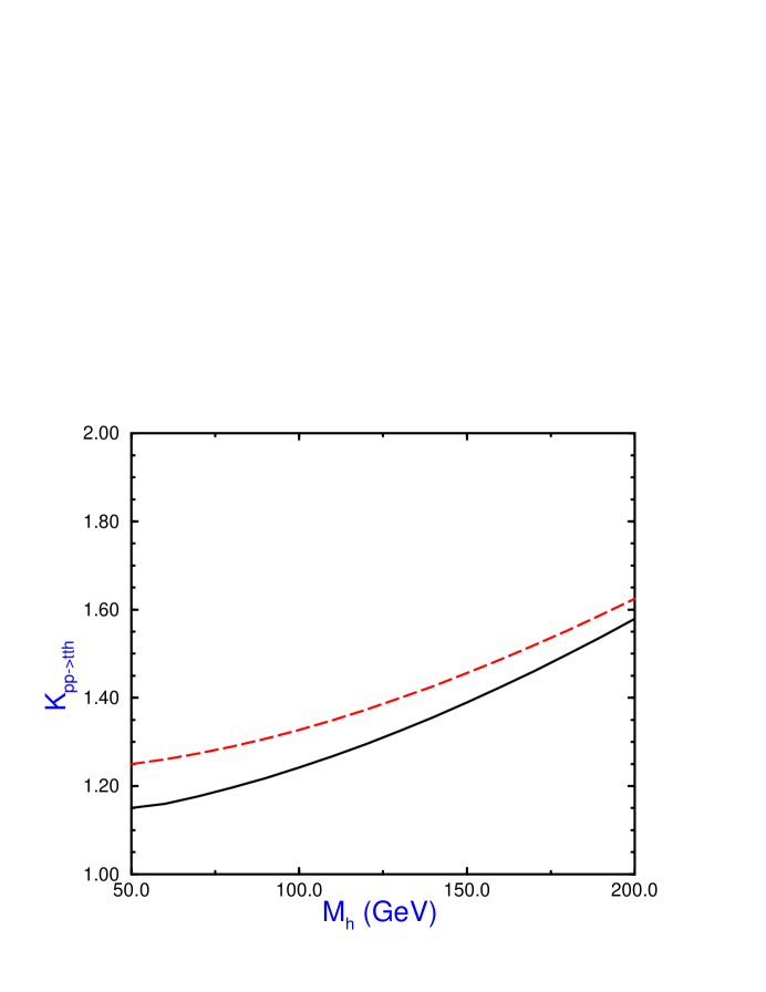
Figure 6: K factor for $pp\rightarrow t\bar{t}h^{0}$ production at the LHC, $\sqrt{s}=14$ TeV, for $\mu=M_{t}$, using Morfin-Tung [18] structure functions. The solid curve uses the $1-$ loop evolution of $\alpha_{s}(\mu)$ and lowest order structure functions for $\sigma^{0}$, and the $2-$loop evolution of $\alpha_{s}(\mu)$ and NLO structure functions for $\sigma^{1}$. The dashed curve uses the $2-$loop evolution of $\alpha_{s}(\mu)$ and the LO structure functions for both $\sigma^{0}$ and $\sigma^{1}$.

4 Conclusions

We have computed the next-to-leading order QCD corrections to $e^{+}e^{-}\rightarrow t\bar{t}h^{0}$ and to $pp\rightarrow t\bar{t}h^{0}$ in the high energy limit and the limit in which $M_{h}<<M_{t}$. We expect this to be a reasonable approximation in the intermediate mass region. The corrections to $e^{+}e^{-}\rightarrow t\bar{t}h^{0}$ are small and can safely be neglected. The corrections to $pp\rightarrow t\bar{t}h^{0}$, however, increase the rate at the LHC by a factor of between $1.2$ to $1.5$ for $M_{h}<180$ GeV, although the numbers are sensitive to the choice of structure functions. Within the context of the EHA, the bulk of these corrections can be identified with the ${\cal O}(\alpha_{s}^{3})$ corrections to the $pp\rightarrow t\bar{t}$ sub-process. The significant size of the corrections underscores the need for a complete calculation.

Appendix A Coefficients for $\sigma(e^{+}e^{-}\rightarrow t\bar{t}h^{0})$

As we have seen in Eq. (36), the differential cross section for $e^{+}e^{-}\rightarrow t\bar{t}h^{0}$ can be expressed in terms of six coefficients $G_{1},\ldots,G_{6}$. Two of them, $G_{1}$ and $G_{2}$ account for the emission of a Higgs from a top quark and are explicitely given by

$$G_{1} = \frac{2\,g_{t}^{2}}{s^{2}\left(\hat{\beta}^{2}-x_{h}^{2}\right)x_{h}}\left(\phantom{\frac{1}{2}}\!\!\!\!-4\hat{\beta}\,\left(4M_{t}^{2}-M_{h}^{2}\right)\,\left(2M_{t}^{2}+s\right)x_{h}+\right.$$

$$\!\!\!\!\!\!\!\!\!\!\!\!\!\!\!\!\!\left.\left(\hat{\beta}^{2}-x_{h}^{2}\right)\left(16M_{t}^{4}+2M_{h}^{4}-2M_{h}^{2}sx_{h}+s^{2}x_{h}^{2}-4M_{t}^{2}\left(3M_{h}^{2}-2s-2sx_{h}\right)\right)\,\log\left({\frac{x_{h}+\hat{\beta}}{x_{h}-\hat{\beta}}}\right)\right)\,\,\,,$$

$$G_{2} = \frac{-2\,g_{t}^{2}}{s^{2}\,\left(\hat{\beta}^{2}-x_{h}^{2}\right)x_{h}}\left(\phantom{\frac{1}{2}}\!\!\!\!\hat{\beta}\,x_{h}\left(-96M_{t}^{4}+24M_{t}^{2}M_{h}^{2}-s\left(-M_{h}^{2}+s+sx_{h}\right)\left(-\hat{\beta}^{2}+x_{h}^{2}\right)\right)\right.+$$

$$\!\!\!\!\!\!\!\!\!\!\!\!\!\!\!\!\!\left.2\left(\hat{\beta}^{2}-x_{h}^{2}\right)\left(24M_{t}^{4}+2\left(M_{h}^{4}-M_{h}^{2}sx_{h}\right)+M_{t}^{2}\left(-14M_{h}^{2}+12sx_{h}+sx_{h}^{2}\right)\right)\log\left(\frac{x_{h}+\hat{\beta}}{x_{h}-\hat{\beta}}\right)\right)\,\,\,,$$

while the other four coefficients, $G_{3},\ldots,G_{6}$ describe the emission of a Higgs from the $Z$-boson and can be written in the following form,

$$G_{3} = \frac{-2\,\hat{\beta}g_{Z}^{2}M_{t}^{2}}{M_{Z}^{2}\left(M_{h}^{2}-M_{Z}^{2}+s-sx_{h}\right)^{2}}\left(4M_{h}^{4}+12M_{Z}^{4}+2M_{Z}^{2}sx_{h}^{2}+s^{2}\left(-1+x_{h}\right)x_{h}^{2}-\right.$$

$$\left.M_{h}^{2}\left(8M_{Z}^{2}+s\left(-4+4x_{h}+x_{h}^{2}\right)\right)\right)\,\,\,,$$

$$G_{4} = \frac{\hat{\beta}g_{Z}^{2}M_{Z}^{2}}{6\left(M_{h}^{2}-M_{Z}^{2}+s-sx_{h}\right)^{2}}\left(48M_{t}^{2}+12M_{h}^{2}-s\left(-24+\hat{\beta}^{2}+24x_{h}-3x_{h}^{2}\right)\right)\,\,\,,$$ (52)

$$G_{5} = \frac{-4\,g_{t}\,g_{Z}\,M_{t}}{M_{Z}\,s\left(-M_{h}^{2}+M_{Z}^{2}+s\left(-1+x_{h}\right)\right)}\left(\phantom{\frac{1}{2}}\!\!\!\!\hat{\beta}\,s\left(6M_{Z}^{2}+x_{h}\left(-M_{h}^{2}-s+sx_{h}\right)\right)+\right.$$

$$\left.2\left(M_{h}^{2}\left(M_{h}^{2}-3M_{Z}^{2}+s-sx_{h}\right)+M_{t}^{2}\left(-4M_{h}^{2}+12M_{Z}^{2}+sx_{h}^{2}\right)\right)\,\log\left({\frac{x_{h}+\hat{\beta}}{x_{h}-\hat{\beta}}}\right)\right)\,\,\,,$$

$$G_{6} = \frac{8\,g_{t}\,g_{Z}\,M_{t}\,M_{Z}}{s\left(-M_{h}^{2}+M_{Z}^{2}+s\,\left(-1+x_{h}\right)\right)}\left(\hat{\beta}\,s+\left(4M_{t}^{2}-M_{h}^{2}+2s-sx_{h}\right)\log\left({\frac{x_{h}+\hat{\beta}}{x_{h}-\hat{\beta}}}\right)\right)\,\,\,\,.$$

In both Eq. (A) and Eq. (A), $g_{t}$ and $g_{Z}$ denote the Yukawa couplings of the top quark ($g_{t}\!=\!M_{t}/v$) and of the $Z$ boson ($g_{Z}\!=\!M_{Z}/v$) respectively, while the quantity $\hat{\beta}$ is defined in Eq. (16). Ref. [15] presents the result for $d\sigma/dx_{1}dx_{2}$, where $x_{1}$ and $x_{2}$ are the fractional energies of the top quarks. After making a change of variables and integrating over $\mid x_{1}-x_{2}\mid$, their expressions for the $G_{i}$ agree with ours.

References

- [1] A. Sopczak, Proceedings of The First International Workshop on Non-Accelerator Physics, Dubna, July, 1997, hep-ph/9712283.
- [2] Z. Kunszt, Nucl. Phys. B247 (1984) 339; D. Dicus and S. Willenbrock, Phys. Rev. D39 (1989) 751; J. Gunion, Phys. Lett. B261 (1991) 510; W. Marciano and F. Paige, Phys. Rev.‘Lett. 66 (1991) 2433; A. Stange, W. Marciano, and S. Willenbrock, Phys. Rev. D50 (1994) 4491.
- [3] T. Han, S. Willenbrock, and G. Valencia, Phys. Rev. Lett. 69 (1992) 3274.
- [4] M. Spira, CERN-TH-97-068, hep-ph/9705337.
- [5] M. Spira, A. Djouadi, D. Graudenz and P. Zerwas, Nucl. Phys. B453 (1995) 17; D. Graudenz, M. Spira, and P. Zerwas, Phys. Rev. Lett. 70 (1993) 1372.
- [6] A. Djouadi, M. Spira, and P. Zerwas, Phys. Lett. B264 1991) 440; S. Dawson, Nucl. Phys. B359 (1991) 283.
- [7] P. Nason, S. Dawson, and R.K. Ellis, Nucl. Phys. B303 (1988) 607.
- [8] W. Beenakker, W. van Neerven, R. Meng, G. Schuler, and J. Smith, Nucl. Phys. B351 (1991) 507; W. Beenakker, H. Kuijf, W. van Neerven, and J. Smith, Phys. Rev. D40 (1989) 54.
- [9] J. Ellis, M. K. Gaillard, and D. Nanopoulos, Nucl. Phys. B106 (1976) 292.
- [10] S. Brodsky, T. Kinoshita, and H. Terazawa, Phys. Rev. D4 (1971) 1532.
- [11] S. Dawson, Nucl. Phys. B249 (1985) 42 ; M. Chanowitz and M. K. Gaillard, Phys. Lett. B142 (1984) 85 ; G. Kane, W. Repko, and W. Rolnick, Phys. Lett. B148 (1984) 367 .
- [12] J.N. Ng and P. Zakarauskas, Phys. Rev. D29 (1984) 876.
- [13] S. Dawson, Phys. Lett. B217 (1989) 347.
- [14] K.J.F. Gaemers and G.J. Gounaris, Phys. Lett. B77 (1978) 379.
- [15] A. Djouadi, J. Kalinowski and P.M. Zerwas, Zeit. Phys. C54 (1992) 255.
- [16] J. Jersák, E. Laermann and P.M. Zerwas, Phys. Rev. D25 (1982) 1218.
- [17] R. Harlander and M. Steinhauser, hep-ph/9710413.
- [18] J. Morfin and W. Tung, Zeit. Phys. C52 (1991) 13.