hep-ph/9712388
JLAB-THY-97-46 Photo– and Electroproduction of $J^{PC}=1^{-+}$ exotics

Abstract

We estimate the kinematic dependence of the exclusive photo– and electroproduction of $J^{PC}=1^{-+}$ exotic mesons due to $\pi$ exchange. We show that the kinematic dependence is largely independent of the exotic meson form factor, which is explicitly derived for a $1^{-+}$ isovector hybrid meson in the flux–tube model of Isgur and Paton. The relevance to experiments currently planned at Jefferson Lab is indicated.

PACS number(s): 12.39.Mk   12.39.Jh   12.40.Nn   12.40.Vv    13.40.Gp   13.60.Le

1 Introduction

Evidence for a $J^{PC}=1^{-+}$ isovector state at 1.4 GeV has been published most recently in $\pi^{-}p\rightarrow\eta\pi^{-}p$ by E852 [2]. Since the $J^{PC}$ of this state is “exotic”, i.e. it implies that it is not a conventional meson, this has raised significant interest in further experimental clarification. Specifically, the advent of high luminosity electron beam facilities like CEBAF at Jefferson Lab have raised the possibility of photo– or electroproducing a $J^{PC}=1^{-+}$ state, leading to two conditionally approved proposals [3, 4].

Experimentally, herculean efforts have been devoted to photoproduce $J^{PC}=1^{-+}$ states, but no partial wave analyses have been reported which would confirm the $J^{PC}$ of the state. Condo et al. claimed an isovector state in $\rho\pi$ with a mass of 1775 MeV and a width of $100-200$ MeV with $J^{PC}$ either $1^{-+},\;2^{-+}$ or $3^{++}$ using a 19.3 GeV photon beam [5]. Enhancements in $b_{1}\pi$ have been reported in a similar mass region with a photon beam of $25-50$ GeV [6] and 19.3 GeV [7].

In this work we perform the first detailed calculation of the photo– and electroproduction of $1^{-+}$ states.

2 Cross–sections

Since diffractive t–channel exchange is usually taken to be C–parity even, it follows by conservation of charge conjugation for electromagnetic and strong interactions that $J^{PC}=1^{-+}$ neutral states cannot be produced by (virtual) photons $\gamma^{\ast}$ via a diffractive mechanism. However, to eliminate the possibility of diffractive exchange completely, we shall specialize to charge exchange, i.e. to $\gamma^{\ast}p\rightarrow{\hat{\rho}}^{+}n$, where ${\hat{\rho}}^{+}$ is an isovector state of mass $M_{{\hat{\rho}}}$ with a neutral isopartner with $J^{PC}=1^{-+}$.

We shall assume in this first orientation that s–channel and u–channel production of states in the mass range of interest are suppressed, since very heavy $\approx M_{{\hat{\rho}}}+M_{p}=2.5-3$ GeV excited nucleons need to be produced for this mechanism to be viable. This leaves us with t–channel meson exchange. The lowest OZI allowed mass exchanges allowed by isospin conservation are $\pi^{+},\;\rho^{+},\;a_{1}^{+}$ and $b_{1}^{+}$. Utilizing vector meson dominance, we note that the $\rho^{+}$ and $b_{1}^{+}$ exchanges require coupling of $\gamma^{\ast}$ to $\omega$, which is suppressed by $(0.30)^{2}=9\%$ relative to the coupling to the $\rho^{0}$ which occurs for the other exchanges [8]. Of the remaining exchanges, $a_{1}^{+}$ is likely to be suppressed due to the large mass of the $a_{1}^{+}$ in its propagator. On the other side, $\pi^{+}$ exchange remains possible, and is generally expected to be especially relevant for a photon at CEBAF energies. The case is further strengthened by noting that there is a large $p\pi^{+}n$ coupling and that there is already experimental evidence from E852 for the $\rho^{0}\pi^{+}$ coupling of a $1^{-+}$ state at 1.6 GeV [9, 10]. In contrast, $\rho^{+}$ exchange is expected to be highly suppressed, at least for hybrid ${\hat{\rho}}$ in the flux–tube model, since the relevant coupling ${\hat{\rho}}^{+}\rightarrow\omega\rho^{+}$, where the photon is regarded as on $\omega$ within VDM, is almost zero [11]. We henceforth restrict to $\pi^{+}$ exchange. At CEBAF energies a single particle rather than a Reggeon picture is appropriate. Nevertheless, we have verified that a Regge theory motivated $t$ dependence does not introduce more sizable corrections to our predicted cross–sections than variations of parameters do.

We write the Lorentz invariant amplitude as [12]

$${\cal M}=eF_{{\hat{\rho}}\gamma\pi}g_{p\pi n}F_{p\pi n}(t)\frac{i}{M_{\pi}^{2}-t}\epsilon_{\mu\nu\alpha\beta}\epsilon_{\mu}^{\gamma}\epsilon_{\nu}^{{\hat{\rho}}\ast}q_{\alpha}^{\gamma}q_{\beta}^{{\hat{\rho}}}{\bar{u}}_{p}\gamma_{5}u_{n}$$ (1)

where $\epsilon$ denotes the polarization vectors of the incoming $\gamma^{\ast}$ and outgoing ${\hat{\rho}}$, $q$ is the corresponding 4–momentum, and $u$ is a bispinor for the initial proton and outgoing neutron. The $\pi$ propagator has the form $i/(M_{\pi}^{2}-t)$, where $t=(q_{p}-q_{n})^{2}$, and we assume a conventional monopole form for the cut–off form factor $F_{p\pi n}(t)=\Lambda^{2}/(\Lambda^{2}-t)$ with $\Lambda=1.2$ GeV. We take the nucleon–$\pi$ coupling constant $g_{p\pi n}=13.5$ [13]. Eq. 1 is the only Lorentz invariant structure that can couple the nucleon to a pseudoscalar exchange (via ${\bar{u}}_{p}\gamma_{5}u_{n}$), and the pseudoscalar to $\gamma^{\ast}$ and ${\hat{\rho}}$ vector particles. As far as the Lorentz structure is concerned, the $\pi$ exchange amplitude for virtual Compton scattering [12], vector meson (e.g. $\rho$) and ${\hat{\rho}}$ production is identical, since the amplitude is not dependent on the C–parity or G–parity of the state. This is the central observation that enables us to link ${\hat{\rho}}$ production with virtual Compton scattering. In fact, we suggest that $\rho^{+}$ photo– and electroproduction should be able to test the results in this work directly in the near future, since diffractive exchange is not possible.

Define four (dimensionless) structure functions for the (unpolarized) $ep\rightarrow e^{{}^{\prime}}{\hat{\rho}}n$ electroproduction cross–section as [12]

$$\frac{d^{5}\sigma}{dE^{{}^{\prime}}d\Omega_{e}d\Omega_{{\hat{\rho}}}}=\frac{\alpha^{2}}{64\pi^{3}}\frac{E^{{}^{\prime}}}{E}\frac{|{\bf q}^{{\hat{\rho}}}|}{M_{p}W}\frac{1}{Q^{2}}\frac{1}{1-\epsilon}[\sigma_{T}+\epsilon\sigma_{L}+\epsilon\cos 2\phi\;\sigma_{TT}+\sqrt{2\epsilon(1+\epsilon)}\cos\phi\;\sigma_{LT}]$$ (2)

$$\epsilon^{-1}=1+2\;\frac{Q^{2}+(E-E^{{}^{\prime}})^{2}}{4EE^{{}^{\prime}}-Q^{2}}$$

where $E(E^{{}^{\prime}})$ is the initial (final) electron energy and $\theta_{e}$ the electron scattering angle in the frame where the proton is at rest. $M_{p}$ is the mass of the proton and $\epsilon$ the virtual photon polarization parameter. $W^{2}=(q_{p}+q_{\gamma})^{2}$ and $Q^{2}=-q_{\gamma}^{2}$. The azimuthal angle $\phi$ and the ${\hat{\rho}}$ angle relative to $\gamma^{\ast}$, $\theta_{c.m.}$, are defined in the centre of mass frame of the target proton and $\gamma^{\ast}$. ¿From Eqs. 1 and 2 the structure functions are

$$\sigma_{T}=[(q_{0}^{{\hat{\rho}}}|{\bf q}^{\gamma}|-|{\bf q}^{{\hat{\rho}}}|q_{0}^{\gamma}\cos\theta_{c.m.})^{2}+(|{\bf q}^{{\hat{\rho}}}|q_{0}^{\gamma}-q_{0}^{{\hat{\rho}}}|{\bf q}^{\gamma}|\cos\theta_{c.m.})^{2}+(q_{0}^{{\hat{\rho}}})^{2}|{\bf q}^{\gamma}|^{2}\sin^{2}\theta_{c.m.}]\;X$$ (3)

$$\sigma_{L}=2|{\bf q}^{{\hat{\rho}}}|^{2}Q^{2}\sin^{2}\theta_{c.m.}\;X$$

$$\sigma_{LT}=2|{\bf q}^{{\hat{\rho}}}|\sqrt{Q^{2}}\;(q_{0}^{{\hat{\rho}}}|{\bf q}^{\gamma}|-|{\bf q}^{{\hat{\rho}}}|q_{0}^{\gamma}\cos\theta_{c.m.})\;\sin\theta_{c.m.}\;X$$

$$\sigma_{TT}=-|{\bf q}^{{\hat{\rho}}}|^{2}(q_{0}^{\gamma})^{2}\sin^{2}\theta_{c.m.}\;X$$

$$X=\frac{-t}{(t-M_{\pi}^{2})^{2}}[F_{{\hat{\rho}}\gamma\pi}g_{p\pi n}F_{p\pi n}]^{2}$$

where $q_{0}$ represents the energies of ${\hat{\rho}}$ and $\gamma^{\ast}$, and ${\bf q}$ the 3–momentum of ${\hat{\rho}}$ and $\gamma^{\ast}$; all in the centre of mass frame of the incoming proton and photon.

As we shall see later, the kinematical dependence of cross–sections will depend only weakly on the ${\hat{\rho}}$ form factor $F_{{\hat{\rho}}\gamma\pi}$. Hence most of the conclusions of this work depend weakly on the details of the (unknown) form factor, and are hence independent of the detailed model assumptions made in the next section. One crucial exception is the absolute magnitude of cross–sections, which depend strongly on the form factor.

3 Flux–tube model form factor for a $1^{-+}$ isovector hybrid

A $1^{-+}$ state cannot be a conventional meson due to its quantum numbers. One possibility is that it is a hybrid meson. This possibility will be further explored here. Extensive hybrid meson decay calculations have been done in the flux–tube model of Isgur and Paton [8, 11]. The model is non–relativistic and is formulated in the rest frame of the hybrid. Since the hybrid form factor is Lorentz invariant it can be evaluated in any frame, particularly the hybrid rest frame. The Lorentz invariant relativistic amplitude, evaluated in the hybrid rest frame for a hybrid of polarization 1, is [13]

$${\cal M}_{R}=eF_{{\hat{\rho}}\gamma\pi}\epsilon_{\mu\nu\alpha\beta}\epsilon_{\mu}^{\gamma}\epsilon_{\nu}^{{\hat{\rho}}\ast}q_{\alpha}^{\gamma}q_{\beta}^{{\hat{\rho}}}=-ieF_{{\hat{\rho}}\gamma\pi}M_{{\hat{\rho}}}|{\bf p}_{\gamma}|$$ (4)

$${\cal M}_{R}=\sqrt{2E_{\pi}\;2E_{\rho}\;2M_{{\hat{\rho}}}}\;{\cal M}_{NR}$$

where we wrote the relativistic amplitude in terms of the non–relativistic amplitude which we shall compute. The meson wave functions are normalized differently in a non–relativistic model than in a relativistic case as shown in Eq. 4. Here $E_{\pi}$ and $E_{\rho}$ (from $\gamma^{\ast}$ via VDM) are the on–shell energies of the $\pi$ and $\rho$, each with momentum $|{\bf p}_{\gamma}|$ in the hybrid rest frame.

The evaluation of the non–relativistic amplitude proceeds as follows. It is taken to be the product of the VDM coupling of $\gamma^{\ast}$ to the $\rho$, the propagator of the $\rho$ and the flux–tube model amplitude for the decay of a $1^{-+}$ hybrid to $\rho\pi$

$${\cal M}_{NR}=\frac{e}{2\gamma_{\rho}}\frac{M_{\rho}^{2}}{M_{\rho}^{2}+Q^{2}}\;\;\mbox{Flux--tube model amplitude}$$ (5)

where $\gamma_{\rho}=2.52$ [8]. The flux–tube model amplitude is evaluated as enunciated in by Close and Page [11], i.e. we assume S.H.O. wave functions for the $\rho$ and $\pi$, with the hybrid wave function and the flux–tube overlap as in ref. [11], except that the small quark–antiquark seperation $r$ behaviour of the hybrid wave function is $\sim r$.

Utilizing Eq. 4 to express the form factor in terms of the relativistic amplitude, and to write this in terms of the non–relativistic amplitude; and using Eq. 5, we obtain

$$F_{{\hat{\rho}}\gamma\pi}=\frac{32\;\pi^{\frac{3}{4}}}{\gamma_{\rho}}\left(\frac{\sqrt{{\bf p}_{\gamma}^{2}+M_{\pi}^{2}}\sqrt{{\bf p}_{\gamma}^{2}+M_{\rho}^{2}}}{M_{{\hat{\rho}}}}\right)^{\frac{1}{2}}\frac{M_{\rho}^{2}}{M_{\rho}^{2}+Q^{2}}\;\frac{0.62\;\gamma_{0}}{(1+\frac{0.2}{\beta_{\pi}^{2}+\beta_{\rho}^{2}})^{2}}$$ (6)

$$\times\frac{(\beta_{\pi}\beta_{\rho})^{\frac{3}{2}}\;\beta_{{\hat{\rho}}}^{\frac{5}{2}}\;(\beta_{\pi}^{2}-\beta_{\rho}^{2})}{(\beta_{\pi}^{2}+\beta_{\rho}^{2})^{\frac{5}{2}}\;\xi^{\frac{5}{2}}}\exp(-\frac{{\bf p}_{\gamma}^{2}}{4\xi})$$

$$\xi=2\beta_{{\hat{\rho}}}^{2}+\frac{1}{2}(\beta_{\pi}^{2}+\beta_{\rho}^{2})-\frac{1}{2}\frac{(\beta_{\pi}^{2}-\beta_{\rho}^{2})^{2}}{\beta_{\pi}^{2}+\beta_{\rho}^{2}}$$

up to a sign. Notice that the pair creation constant $\gamma_{0}$ of the ${}^{3}P_{0}$ model enters explicitly in Eq. 6. This is because the flux–tube model, within the assumptions made for the wave functions, gives a prediction for the couplings of a hybrid in terms of couplings for mesons in the ${}^{3}P_{0}$ model [11]. We use $\gamma_{0}=0.53$ which reproduces conventional meson decay phenomenology [14]. In Eq. 6, $\beta$ refers to the inverse radius of the state, the parameter that enters in the wave function. Due to the $\beta_{\pi}^{2}-\beta_{\rho}^{2}$ term, we note that if $\beta_{\pi}=\beta_{\rho}$ the form factor vanishes, which explicitly exforces the selection rule that hybrid coupling to two S–wave mesons is suppressed [11].

Figure 1: Structure function $\sigma_{T}$ at $W=3$ GeV with standard parameters. $Q^{2}$ is varied within its kinematically allowed range for $E=6$ GeV.

4 Electroproduction results

We utilize the “standard parameters” $M_{{\hat{\rho}}}=1.8$ GeV, $\beta_{{\hat{\rho}}}=0.27$ GeV [11], $\beta_{\rho}=0.31$ GeV and $\beta_{\pi}=0.54$ GeV [15].

All the kinematical variables that the structure functions depend on, introduced in Eqs. 2, 3 and 6, can be expressed as functions of the Lorentz invariant variables $Q^{2}$ and $W$, and $\theta_{c.m.}$ (see Appendix).

Figure 2: Structure function $\sigma_{T}$ for $Q^{2}=0$ and the $\Sigma$ asymmetry of photoproduction with standard parameters. $W$ is varied within its kinematically allowed range for $E=6$ GeV.

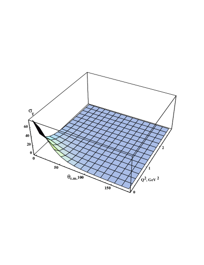
The structure function $\sigma_{T}$ is plotted in Figure 1 for $W=3$ GeV. $\sigma_{T}$ is the most dominant structure function: it peaks strongly at small $Q^{2}$ and $\theta_{c.m.}$. Physically, $Q^{2}=0$ corresponds to the incoming and outgoing electrons moving in the same direction. $\theta_{c.m.}=0$ corresponds to the photon and the ${\hat{\rho}}$ moving in the same direction. Hence $\sigma_{T}$ peaks where the ${\hat{\rho}}$ goes in the same direction as the incoming electron, i.e. towards the beam pipe. This becomes especially critical when there is a sizable “hole” in the detector, which is the case for the CLAS spectrometer at CEBAF. The other three structure functions are small when compared to $\sigma_{T}$, with a suppression factor of about $10^{-3}$ for $\sigma_{L}$ and $10^{-2}$ for $\sigma_{LT}$ and $\sigma_{TT}$. These three structure functions also peak at small $Q^{2}$ and $\theta_{c.m.}$. Experiments should be optimized to enable detection at small $Q^{2}$ and $\theta_{c.m.}$. According to the Appendix (Eq. 14), $\theta_{c.m.}=0$ corresponds to the minimal value of $|t|$, so that peaking of cross–sections at small $|t|$ would be a strong experimental test for the $\pi^{+}$ exchange explored here, especially since other exchanges are expected to be more substantial at larger $|t|$.

As we pointed out, the structure function due to longitudinal photons $\sigma_{L}$ is tiny. Correspondingly, $\sigma_{LT}$ which is due to interference between longitudinal and transverse photons is smaller than $\sigma_{T}$. The reason for this is that longitudinal photons give no contribution to the process in a typical case: when ${\hat{\rho}}$ is at rest the amplitude $\epsilon_{\mu\nu\alpha\beta}\epsilon_{\mu}^{\gamma}\epsilon_{\nu}^{{\hat{\rho}}\ast}q_{\alpha}^{\gamma}q_{\beta}^{{\hat{\rho}}}$ in Eq. 1 vanishes. The suppression of contributions from longitudinal photons need not be true for exchanges other than $\pi^{+}$ exchange.

Figure 3: Structure function $\sigma_{T}$ for $\theta_{c.m.}=0$ with standard parameters. If a curve is drawn from the top to the bottom corner described by $Q^{2}=Q^{2}_{max}$ (see Eq. A), then the region to the left of the curve corresponds to the physically accessible region of parameter space for $E=6$ GeV.

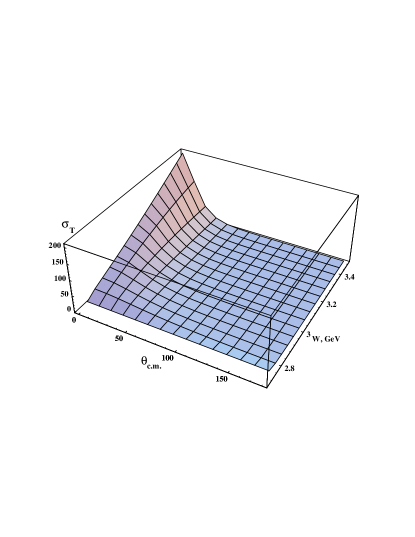
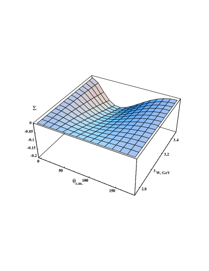
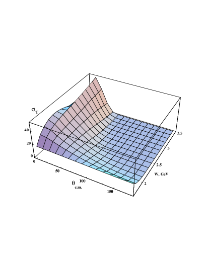
In Figure 2 we show the non–zero structure functions for $Q^{2}=0$ corresponding to real (transversely polarized) photons. Again $\sigma_{T}$ is dominant. Both $\sigma_{T}$ and $\sigma_{TT}$ peak at large $W$ as would be expected because large $W$ corresponds to an increase of phase space for the production of the ${\hat{\rho}}$. We also plot the photoproduction asymmetry parameter $\Sigma=\sigma_{TT}/\sigma_{T}$, which can be accessed by using linearly polarized photons. Note that $\Sigma=0$ at the reaction threshold.

Figure 4: The difference (in percent) between the structure function $\sigma_{T}$ with the test form factor (denoted $\sigma_{T}^{{{test}}}$) and $\sigma_{T}$ with the flux–tube model form factor for standard parameters as a function of $Q^{2},W$ and $\theta_{c.m.}$, varied within their kinematically allowed ranges for $E=6$ GeV. We normalize the test form factor to agree with the flux–tube model form factor at points where $\sigma_{T}$ is maximal, denoted $\sigma_{{{max}}}$. For the first graph $W=3$ GeV, and for the second $Q^{2}=0$. The “difference” is defined as $(\sigma_{T}^{{{test}}}\;\sigma_{{{max}}}/\sigma_{{{max}}}^{{{test}}}\;-\sigma_{T})/\sigma_{{{max}}}$.

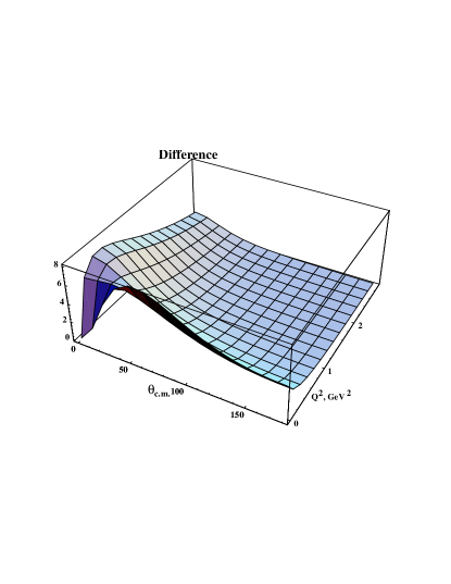
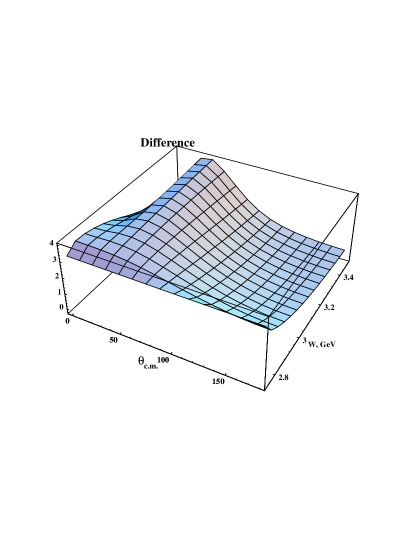
Figure 3 shows the non–zero structure function for $\theta_{c.m.}=0$, where $\sigma_{T}$ attains its maximum and the negative value $t\neq 0$ is nearest to $0$.

We define a typical test form factor based on $\rho$ dominance as

$$F_{{\hat{\rho}}\gamma\pi}\propto\frac{1}{M_{\rho}^{2}+Q^{2}}$$ (7)

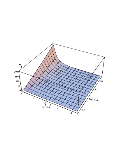
We have evaluated the structure functions for the test form factor in Eq. 7. Remarkably, for all values of $Q^{2},W$ and $\theta_{c.m.}$ the form of the structure functions are very similar, even though the form factors in Eqns. 6 and 7 have different functional dependence on different parameters. This is demonstrated for the dominant structure function $\sigma_{T}$ in Figure 4, where we see that the difference is a few percent. Thus the $Q^{2},W$ and $\theta_{c.m.}$ dependence of the cross–section in Eq. 2 is very weakly dependent on models for $F_{{\hat{\rho}}\gamma\pi}$, so that the kinematic dependence of total cross–sections, and hence many conclusions of this work, are independent of the details of specific models. This happens because the Lorentz structure of one $\pi$ exchange (Eq. 1), and not the form factor, governs kinematical dependence.

We shall now evaluate the total cross–section by integrating over all kinematical variables in their allowed ranges, except for the following. The electron scattering angle $\theta_{e}$ is assumed to be larger than $\theta_{e}^{min}$, and $E^{{}^{\prime}}$ is assumed to be larger than $0.1$ GeV. From a theoretical viewpoint, these conditions ensure that we do not reach $\theta_{e}=0$ and $E^{{}^{\prime}}=0$ where the cross–section in Eq. 2 diverges. Experimentally, the outgoing electron is usually detected for $\theta_{e}>\theta_{e}^{min}$. There are also experimental limits on detection of small outgoing electron energies.

For the total cross–section, the results are shown in Table 1. The decrease of cross–section for increased ${\hat{\rho}}$ mass is due to the decrease in available phase space. The decrease of cross–section with increasing electron energy is due to the “hole” in the forward direction through which an ever increasing number of electrons pass. The qualitative dependence of the cross–section on $E$ is also found for the test form factor, and is hence mostly model independent. One of the implications of Table 1 is that for the CLAS detector at CEBAF, an electron beam towards the lower end of the range (e.g. 5.5 GeV) appears to be preferable. Another implication is that at DESY HERA with a 27.52 GeV proton beam and 820 GeV electron beam, corresponding to $E=48.1$ TeV, $1^{-+}$ ${\hat{\rho}}$ production should be negligible.

Table 1: Total electroproduction cross–section in $pb$ for $\theta_{e}^{min}=12^{o}$ and $E^{{}^{\prime}}$ larger than $0.1$ GeV, relevant to the CLAS detector at CEBAF. We utilize the standard parameters.

Electron Energy	${\hat{\rho}}$ Mass
(GeV)	1.4 GeV	1.8 GeV	2.2 GeV
5.5	62	29	3.7
6	50	28	6.5
6.5	41	25	7.9
8	21	16	7.8
20	0.6	0.5	0.4

We have also computed the total cross–section for various values of $\theta_{e}^{min}$ and obtain

$\theta_{e}^{min}$	Total cross–section ($pb$)
$12^{o}$	28
$5^{o}$	110
$1^{o}$	360

so that the cross–section increases substantially as the “hole” in the detector becomes smaller. This implies that improved statistics for ${\hat{\rho}}$ should result from the ability to put detectors as near as possible to the beam pipe in the forward direction.

It is of interest to check the total cross–section as a function of the wave function parameters of the participating conventional mesons for $\theta_{e}^{min}=12^{o}$.

	Total cross–section ($pb$)
Standard parameters	28
$\beta_{\rho}=0.45$ GeV and $\beta_{\pi}=0.75$ GeV [16]	15

We note that the cross–section changed by a factor of two if the two conventional meson wave function parameters are changed to reasonable values. Also, we chose a value of $\gamma_{0}$ towards the upper end of the range in the literature [14]. In calculations of excited mesons, values of $\gamma_{0}^{2}$ that are 50% lower have been used. Hence, within this model, revisions in the $\beta$’s and $\gamma_{0}$ can make the cross–sections $\sim 30\%$ of the values quoted for electroproduction cross–sections in this section and Table 1. Hence absolute cross–sections should be regarded with more caution than kinematic dependence.

To summarize this section, we stress that the $t$-channel $\pi$ exchange mechanism of $1^{-+}$ electroproduction leads to dominance of transverse photoabsorption. Therefore a Rosenbluth–type separation of different structure functions contributing to the cross section would be necessary in order to understand the ${\hat{\rho}}$ electroproduction mechanism.

5 Photoproduction results

The photoproduction cross–section ($Q^{2}=0$) is

$$\frac{d\sigma_{\gamma}}{d\Omega_{c.m.}}=\frac{\alpha}{16\pi}\frac{|{\bf q}^{{\hat{\rho}}}|}{M_{p}(W^{2}-M_{p}^{2})}(\sigma_{T}+\epsilon\cos 2\phi\sigma_{TT}),$$ (8)

where $\phi$ is the angle defined by the planes of photon linear polarization and ${\hat{\rho}}$ production; and the parameter $\epsilon$ defines the degree of photon linear polarization. The total photoproduction cross–section may be obtained by integrating the preceding formula over $\Omega_{c.m.}$,

$$\sigma_{\gamma}=\frac{\alpha}{8}\frac{|{\bf q}^{{\hat{\rho}}}|}{M_{p}(W^{2}-M_{p}^{2})}\int\sigma_{T}\sin\theta_{c.m.}\ d{\normalsize\theta_{c.m.}},$$ (9)

Figure 5: Photoproduction cross–section in $nb$ as a function of photon energy (in GeV) for various ${\hat{\rho}}$ masses for standard parameters. From top to bottom on the vertical axis this corresponds to ${\hat{\rho}}$ masses of 1.4, 1.8 and 2.2 GeV.

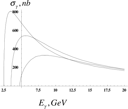
The photoproduction cross–section $\sigma_{\gamma}$ is shown in Figure 5. The cross–section peaks not far from the ${\hat{\rho}}$ production threshold. The shape of the cross–section as a function of photon energy is very similar for the test form factor.

The reason for the fall in the photoproduction cross–section with increasing photon energy is firstly that, as the photon energy increases, the smallest allowed $|t|$ (where the cross–sections peak) decreases, so that $q_{\alpha}^{\gamma}\approx q_{\beta}^{{\hat{\rho}}}$ and the factor $\epsilon_{\mu\nu\alpha\beta}\epsilon_{\mu}^{\gamma}\epsilon_{\nu}^{{\hat{\rho}}\ast}q_{\alpha}^{\gamma}q_{\beta}^{{\hat{\rho}}}$ in the amplitude vanishes. Secondly, the $\gamma_{5}$ coupling of the $\pi^{+}$ to the proton and neutron is such that it flips the spin of the nucleon. As $t\rightarrow 0$ the proton and neutron 4–momenta become identical and the spin flip would become zero, so that the amplitude $\sim t$ (as can be seen explicitly in Eq. 3). This means that with increasing photon energy the spin flip of the nucleon suppresses the cross–section.

We check the total cross–section as a function of the wave function parameters of the participating conventional mesons for 6 GeV photons and ${\hat{\rho}}$ of mass 1.8 GeV.

	Total cross–section ($nb$)
Standard parameters	540
$\beta_{\rho}=0.45$ GeV and $\beta_{\pi}=0.75$ GeV [16]	250

Hence, within this model revisions in the $\beta$’s and $\gamma_{0}$ can make the cross–sections $\sim 25\%$ of the values quoted for photoproduction cross–sections in Figure 5.

We have already suggested that $\rho^{+}$ electro– and photoproduction can test the ideas in this work. Unfortunately the relevant data for $\rho^{+}$ has not yet been taken and only $\rho^{+}$ inclusive photoproduction data exist [17]. Photoproduction data is the most likely to be forthcoming, and we show the dominant structure function $\sigma_{T}$ in Figure 6. It may be observed that the structure function is somewhat different from the ${\hat{\rho}}$ structure function in Figure 2. This is mainly due to the fact that the mass of the $\rho$ is very different from the ${\hat{\rho}}$. We find that the $\rho$ structure functions $\sigma_{L},\;\sigma_{LT}$ and $\sigma_{TT}$ have similar parameter dependence to their ${\hat{\rho}}$ analogues.

Figure 6: The $W$ and $\theta_{c.m.}$ dependence of the structure function $\sigma_{T}$ for $\rho^{+}$ production at $Q^{2}=0$. We vary $W$ within its kinematically allowed range for $E=6$ GeV. Within the framework of VDM, $\gamma^{\ast}$ couples to an $\omega$, and the $\omega$ couples to the $\rho^{+}$ and $\pi^{+}$ via G-parity allowed OZI allowed couplings. The structure functions are those of Eq. 3 with all references to ${\hat{\rho}}$ replaced by $\rho$. The flux–tube model form factor for $\rho^{+}$ production is proportional to the form factor in Eq. 6 with the understanding that all reference to $\rho$ is replaced by $\omega$, and all reference to ${\hat{\rho}}$ is replaced with $\rho$. We use Eq. 6 with $\beta_{\rho}=\beta_{\omega}=0.31$ GeV and $\beta_{\pi}=0.54$ GeV. The normalization of the structure function has hence been chosen to coincide with its analogue in Figure 2 to facilitate comparison; and has no physical significance.

6 Summary

$\bullet$ We found that the electroproduction cross–section peaks at small $Q^{2}$, $\theta_{c.m.}$ and large $W$, with the consequence that it is strongly enhanced for small–angle electron scattering.

$\bullet$ The kinematical dependence of cross–sections only weakly depends on the model–dependent form factor of the $\gamma\pi\to 1^{-+}$ transition. The conclusions drawn can also be tested in $\rho^{+}$ electro– and photoproduction.

$\bullet$ A Rosenbluth–type separation of electroproduction cross section and $\Sigma$–asymmetry measurements in photoproduction are necessary to verify the ${\hat{\rho}}$ production mechanism.

$\bullet$ The $1^{-+}$ photoproduction cross–section peaks at energies near to the reaction threshold and reaches values around 0.3 to 0.8 $\mu$b depending on model parameters and the assumed mass of the ${\hat{\rho}}$ meson.

7 Conclusion

We conclude that electro- and photoproduction of $1^{-+}$ exotic mesons from a proton target has high enough cross sections to be observed in forthcoming Jefferson Lab experiments. Optimal conditions to study ${\hat{\rho}}$ photoproduction would require a high intensity beam of real (or quasi–real) photons with variable energies between 2.5 and 10 GeV, assuming that the (still unknown) ${\hat{\rho}}$ mass is within the range of 1.4 to 2.2 GeV.

Acknowledgements

Helpful discussions with G. Adams, A. Donnachie and S. Stepanyan are acknowledged. We specifically thank Nathan Isgur for encouragement. The work of A.A. was supported by the US Department of Energy under contract DE–AC05–84ER40150. P.R.P. acknowledges a Lindemann Fellowship from the English Speaking Union.

Appendix A Appendix: Relationships between kinematical variables

$Q^{2}$ and $W$ are related to $E^{{}^{\prime}}$ and $\theta_{e}$ by

$$Q^{2}=2EE^{{}^{\prime}}(1-\cos\theta_{e})\hskip 28.45274ptW^{2}=-2EE^{{}^{\prime}}(1-\cos\theta_{e})+2M_{p}(E-E^{{}^{\prime}})+M_{p}^{2}$$ (10)

where $0\leq Q^{2}\leq Q^{2}_{max}$ and $M_{n}+M_{{\hat{\rho}}}\leq W\leq\sqrt{M_{p}(M_{p}+2E)}$; and $0\leq\theta_{e}\leq\pi$ and $0\leq E^{{}^{\prime}}\leq E_{max}^{{}^{\prime}}$, with

$$Q^{2}_{max}=\frac{2E}{M_{p}+2E}(M_{p}^{2}+2M_{p}E-W^{2})$$

$$E_{max}^{{}^{\prime}}=\frac{M_{p}E+\frac{1}{2}M_{p}^{2}-\frac{1}{2}(M_{n}+M_{{\hat{\rho}}})^{2}}{E(1-\cos\theta_{e})+M_{p}}$$ (11)

The variables $q_{0}^{{\hat{\rho}}},|{\bf q}^{{\hat{\rho}}}|$ and $q_{0}^{\gamma},|{\bf q}^{\gamma}|$ are defined in terms of $W$ and $Q^{2}$ by

$$q_{0}^{{\hat{\rho}}}=\sqrt{|{\bf q}^{{\hat{\rho}}}|^{2}+M_{{\hat{\rho}}}^{2}}=\frac{W^{2}+M_{{\hat{\rho}}}^{2}-M_{n}^{2}}{2W}$$

$$q_{0}^{\gamma}=\sqrt{|{\bf q}^{\gamma}|^{2}-Q^{2}}=\frac{-Q^{2}+W^{2}-M_{p}^{2}}{2W}$$ (12)

${\bf p}_{\gamma}$ can be written in terms of $Q^{2},\;W$ amd $t$ as

$${\bf p}_{\gamma}^{2}=\frac{M_{{\hat{\rho}}}^{4}+Q^{4}+t^{2}+2M_{{\hat{\rho}}}^{2}Q^{2}-2M_{{\hat{\rho}}}^{2}t+2Q^{2}t}{4M_{{\hat{\rho}}}^{2}}$$ (13)

where

$$t=(-q_{0}^{\gamma}+q_{0}^{{\hat{\rho}}})^{2}-(|{\bf q}^{\gamma}|^{2}+|{\bf q}^{{\hat{\rho}}}|^{2}-2|{\bf q}^{\gamma}||{\bf q}^{{\hat{\rho}}}|\cos\theta_{c.m.})$$ (14)

For photoproduction, the photon energy is

$$E_{\gamma}=\frac{W^{2}-M_{p}^{2}}{2M_{p}}$$ (15)