Four-jet angular distributions and color charge measurements: leading order versus next-to-leading order

Abstract

We present the next-to-leading order perturbative QCD prediction to the four-jet angular distributions used by experimental collaborations at LEP for measuring the QCD color charge factors. We compare our results to ALEPH data corrected to parton level. We perform a leading order “measurement” of the QCD color factor ratios by fitting the leading order perturbative predictions to the next-to-leading order result. Our result shows that in an experimental analysis for measuring the color charge factors the use of the O($\alpha_{s}^{3}$) QCD predictions instead of the O($\alpha_{s}^{2}$) results may shift the center of the fit by a relative factor of $1+2{\alpha_{s}}$ in the $T_{R}/C_{F}$ direction.

I Introduction

In the first phase of operation of the Large Electron Positron Collider (LEP) four-jet events were primarily used for measuring the eigenvalues of the Casimir operators of the underlying symmetry group, the QCD color factors [1, 2, 3, 4, 5]. The values of these color charges test whether the dynamics is indeed described by an SU(3) symmetry. The dependence of jet cross sections on the adjoint color charge appear at O($\alpha_{s}^{2}$). Several test variables with perturbative expansion starting at O($\alpha_{s}^{2}$) — so called four-jet angular distributions — were proposed as candidate observables with particular sensitivity to the gauge structure of the theory [2, 6, 7, 8]. For a long time, however, perturbative QCD prediction for these variables at O($\alpha_{s}^{3}$) had not been available, therefore the absolute normalization of the perturbative prediction could not be fixed. In order to circumvent this problem the experimental collaborations either fitted the strong coupling as well, or used normalized angular distributions of four jet events that were expected to be insensitive to renormalization scale dependence. The small scale dependence however, is but an indication and not a proof of negligible radiative corrections: in principle the shape of the distribution can change from O($\alpha_{s}^{2}$) to O($\alpha_{s}^{3}$). Therefore, it is desirable to check explicitly the effect of the next-to-leading order corrections on these normalized angle distributions.

Recently the next-to-leading order corrections to various four-jet observables have been calculated [9, 10, 11]. These works depend crucially on the matrix elements for the relevant QCD subprocesses, i.e. for the $e^{+}e^{-}\to{\bar{q}}qgg$ and $e^{+}e^{-}\to{\bar{q}}q{\bar{Q}}Q$ processes at one loop and for the $e^{+}e^{-}\to{\bar{q}}qggg$ and $e^{+}e^{-}\to{\bar{q}}q{\bar{Q}}Qg$ processes at tree level. The loop results became available due to the effort of two groups. In refs. [12, 13] Campbell, Glover and Miller made FORTRAN programs for the next-to-leading order squared matrix elements of the $e^{+}e^{-}\to\gamma^{*}\to{\bar{q}}q{\bar{Q}}Q$ and ${\bar{q}}qgg$ processes publicly available. In refs. [14, 15] Bern, Dixon, Kosower and Wienzierl gave analytic formulæ for the helicity amplitudes of the same processes with the $e^{+}e^{-}\to Z^{0}\to$ four partons channel included as well. The helicity amplitudes for the five-parton processes have been known for a long time [16]. Using the helicity amplitudes in refs. [14, 15, 16], Dixon and Signer calculated the next-to-leading order corrections to four-jet fractions for various clustering algorithms [9], as well as to the $\chi_{\rm BZ}$ angle distribution [10]. In previous publications we calculated several four-jet shape variables at the next-to-leading order accuracy [11]. In this paper we calculate the radiative corrections to the distributions of the commonly used angular shape variables $\phi_{{\rm KSW}}$, $\theta^{*}_{{\rm NR}}$, $\alpha_{{\rm 34}}$, and repeat the calculation for the distribution of $\chi_{{\rm BZ}}$. We use the matrix elements of refs. [14, 15] for the loop corrections, while calculated the helicity amplitudes of the relevant tree-level processes ourselves.

Knowing the next-to-leading order corrections to these angular distributions, one would like to quantify their effect on the measurement of the QCD color charges. We estimate the systematic error coming from the use of leading order results instead of the next-to-leading order one in the fits for the color charge ratios $x=C_{A}/C_{F}$ and $y=T_{R}/C_{F}$ in the following way. We assume that next-to-leading order QCD is the true theory that describes the data. We fit the leading order prediction of the angular distributions with $x$ and $y$ left free to our next-to-leading order QCD results and determine these charge ratios from this fit. The central value of the “measured” charge ratios differs from the SU(3) values $x=9/4$ and $y=3/8$. This shift is the systematic bias that comes from the use of leading order fits in experimental analyses instead of the next-to-leading order ones.

The rest of the paper is organized as follows. In section II we outline the structure of the numerical calculation and describe how we parametrise our results. In section III we present the complete O($\alpha_{s}^{3}$) predictions for the four standard angular distributions using two different jet algorithms: the Durham algorithm [17] and the Cambridge algorithm proposed recently [18]. In section IV we perform the leading order fit of the color charges to our next-to-leading order results. Section V contains our conclusions.

II The structure of the numerical calculation

It is well known that the next-to-leading order correction is a sum of two integrals — the real and virtual corrections — that are separately divergent (in the infrared) in $d=4$ dimensions. For infrared safe observables, for instance the four-jet angular distributions used in this work, their sum is finite. In order to obtain this finite correction, we use a slightly modified version of the dipole method of Catani and Seymour [19] that exposes the cancellation of the infrared singularities directly at the integrand level. The formal result of this cancellation is that the next-to-leading order correction is a sum of two finite integrals,

$$\sigma^{\rm NLO}=\int_{5}{\rm d}\sigma_{5}^{\rm NLO}+\int_{4}{\rm d}\sigma_{4}^{\rm NLO}\>,$$ (1)

where the first term is an integral over the available five-parton phase space (as defined by the jet observable) and the second one is an integral over the available four-parton phase space.

Once the phase space integrations in eq. (1) are carried out, the next-to-leading order differential cross section for the four-jet observable $O_{4}$ takes the general form

$$\frac{1}{\sigma_{0}}\frac{{\rm d}\sigma}{{\rm d}O_{4}}(O_{4})=\left(\frac{{\alpha_{s}}(\mu)C_{F}}{2\pi}\right)^{2}B_{O_{4}}(O_{4})+\left(\frac{{\alpha_{s}}(\mu)C_{F}}{2\pi}\right)^{3}\left[B_{O_{4}}(O_{4})\frac{\beta_{0}}{C_{F}}\ln\frac{\mu^{2}}{s}+C_{O_{4}}(O_{4})\right]\>.$$ (2)

In this equation $\sigma_{0}$ denotes the Born cross section for the process $e^{+}e^{-}\to{\bar{q}}q$, $s$ is the total c.m. energy squared, $\mu$ is the renormalization scale, while $B_{O_{4}}$ and $C_{O_{4}}$ are scale independent functions, $B_{O_{4}}$ is the Born approximation and $C_{O_{4}}$ is the radiative correction. We use the two-loop expression for the running coupling,

$${\alpha_{s}}(\mu)=\frac{{\alpha_{s}}(M_{Z})}{w(\mu)}\left(1-\frac{\beta_{1}}{\beta_{0}}\frac{{\alpha_{s}}(M_{Z})}{2\pi}\frac{\ln(w(\mu))}{w(\mu)}\right)\>,$$ (3)

with

$$w(\mu)=1-\beta_{0}\frac{{\alpha_{s}}(M_{Z})}{2\pi}\ln\left(\frac{M_{Z}}{\mu}\right)\>,$$ (4)

$$\beta_{0}=\frac{11}{3}C_{A}-\frac{4}{3}T_{R}{N_{\rm f}}\>,$$ (5)

$$\beta_{1}=\frac{17}{3}C_{A}^{2}-2C_{F}T_{R}{N_{\rm f}}-\frac{10}{3}C_{A}T_{R}{N_{\rm f}}\>,$$ (6)

with the normalization $T_{R}=1/2$ in ${\rm Tr}(T^{a}T^{{\dagger}b})=T_{R}\delta^{ab}$. The numerical values presented in this letter were obtained at the $Z^{0}$ peak with $M_{Z}=91.187$ GeV, $\Gamma_{Z}=2.49$ GeV, $\sin_{W}^{2}\theta=0.23$, ${\alpha_{s}}(M_{Z})=0.118$ and ${N_{\rm f}}=5$ light quark flavors.

The Born approximation and the higher order correction are linear and quadratic forms of ratios of the color charges [20]:

$$B_{4}=B_{0}+B_{x}\,x+B_{y}\,y\>,$$ (7)

and

$$C_{4}=C_{0}+\,C_{x}\,x+C_{y}\,y+C_{z}\,z+\,C_{xx}\,x^{2}+C_{xy}\,x\,y+C_{yy}\,y^{2}\>.$$ (8)

At next-to-leading order the ratio $z$ appears that is related to the square of a cubic Casimir,

$$C_{3}=\sum_{a,b,c=1}^{N_{A}}{\rm Tr}(T^{a}T^{b}T^{{\dagger}c}){\rm Tr}(T^{{\dagger}c}T^{b}T^{a})\>,$$ (9)

via $z=\frac{C_{3}}{{N_{C}}C_{F}^{3}}$. The Born functions $B_{i}$ are obtained by integrating the fully exclusive O($\alpha_{s}^{2}$) ERT matrix elements [21] and were used by the experimental collaborations [1, 2, 3, 4, 5]. In the next section we present the $C_{i}$ correction functions for the four different angular distributions.

III Results

In order to define the angular variables we denote the three-momenta of the four jets by $\vec{p}_{i}$, ($i=1,2,3,4$) and label jets in order of descending jet energy, such that jet 1 has the highest energy and jet 4 has the smallest. The four variables are

1. the Körner-Schierholz-Willrodt variable [6],$\cos\phi_{{\rm KSW}}$ is the cosine of the average of two angles between planes spanned by the jets,

   $$\phi_{{\rm KSW}}=\frac{1}{2}\left[\arccos\left(\frac{(\vec{p}_{1}\times\vec{p}_{4})\cdot(\vec{p}_{2}\times\vec{p}_{3})}{|\vec{p}_{1}\times\vec{p}_{4}||\vec{p}_{2}\times\vec{p}_{3}|}\right)+\arccos\left(\frac{(\vec{p}_{1}\times\vec{p}_{3})\cdot(\vec{p}_{2}\times\vec{p}_{4})}{|\vec{p}_{1}\times\vec{p}_{3}||\vec{p}_{2}\times\vec{p}_{4}|}\right)\right]\>;$$ (10)

2. the modified Nachtmann-Reiter variable [7], $|\cos\theta^{*}_{{\rm NR}}|$ is the absolute value of the cosine of the angle between the vectors $\vec{p}_{1}-\vec{p}_{2}$ and $\vec{p}_{3}-\vec{p}_{4}$,

   $$\cos\theta^{*}_{{\rm NR}}=\frac{(\vec{p}_{1}-\vec{p}_{2})\cdot(\vec{p}_{3}-\vec{p}_{4})}{|\vec{p}_{1}-\vec{p}_{2}||\vec{p}_{3}-\vec{p}_{4}|}\>;$$ (11)

3. $\cos\alpha_{{\rm 34}}$ [2], the cosine of the angle between the two smallest energy jets,

   $$\cos\alpha_{{\rm 34}}=\frac{\vec{p}_{3}\cdot\vec{p}_{4}}{|\vec{p}_{3}||\vec{p}_{4}|}\>;$$ (12)

4. the Bengtsson-Zerwas correlation [8], $|\cos\chi_{{\rm BZ}}|$ is the absolute value of the cosine of the angle between the plane spanned by jets 1 and 2 and that by jets 3 and 4,

   $$\cos\chi_{{\rm BZ}}=\frac{(\vec{p}_{1}\times\vec{p}_{2})\cdot(\vec{p}_{3}\times\vec{p}_{4})}{|\vec{p}_{1}\times\vec{p}_{2}||\vec{p}_{3}\times\vec{p}_{4}|}\>;$$ (13)

We tabulate the numerical value of the next-to-leading order kinematic functions for these angular variables in the Appendix in Tables III–VI for the Durham clustering algorithm and in Tables VII–X for the Cambridge algorithm that was proposed recently [18]. Using this new algorithm, the hadronization corrections are expected to be much smaller therefore, the perturbative prediction is more reliable. The values in the tables were obtained by selecting four-jet events at a fixed jet resolution parameter $y_{\rm cut}=0.008$ which is the value used by the ALEPH collaboration [5]. We do not show the value of the $C_{z}$ functions because they turn out to be negligible. The $C_{4}$ values were obtained according to eq. (8) with SU(3) values for the color charge ratios, $x=9/4$, $y=3/8$. Comparing the size of the corrections for these two algorithms, we see that in general the $C_{i}$ functions in the case of the Cambridge algorithm are 10–20 % smaller.

We use the numerical values for the kinematic functions to calculate the next-to-leading order QCD predictions for the SU(3) values $x=9/4$, $y=3/8$ according to eq. (2) at $x_{\mu}=\mu/\sqrt{s}=1$. We compare our predictions for the Durham algorithm (solid histograms) to ALEPH data (diamonds) in Figs. 1–4. In order to make this comparison we normalize the histograms to one, therefore

$$F(z)=\frac{1}{\sigma}\frac{{\rm d}\sigma}{{\rm d}z}(z)$$ (14)

in the plots. The qualitative agreement between data and theory is very good. Also shown in these figures our results for the Cambridge algorithm (dotted histograms). The statistical error of the Monte Carlo integrals is below 1.5 % for the Durham algorithm and below 2 % in the case of the Cambridge algorithm in each of the bins. In the same figures, the windows show polinomial fits to the $K$ factors of the normalized distributions defined as

$$K(z)=\frac{1}{\sigma_{{\rm NLO}}}\frac{{\rm d}\sigma_{{\rm NLO}}}{{\rm d}z}(z)\Bigg{/}\frac{1}{\sigma^{{\rm LO}}}\frac{{\rm d}\sigma^{{\rm LO}}}{{\rm d}z}(z)\>,$$ (15)

where $\sigma_{\rm NLO}=\sigma^{\rm LO}+\sigma^{\rm NLO}$ is the next-to-leading order cross section. The $\chi^{2}/N_{\rm dof}$ of these fits is between (1.5–7)/20. The $K$ factors for the $|\cos\chi_{{\rm BZ}}|$ distributions, for the $\cos\alpha_{{\rm 34}}$ distribution with Durham algorithm and for the $|\cos\theta^{*}_{{\rm NR}}|$ distribution with the Cambridge algorithm are approximately constant 1 over the whole range, therefore the shape of the leading and next-to-leading order distributions are very similar in these cases.

FIG. 1.: Comparison of the next-to-leading order QCD prediction for the $\cos\phi_{{\rm KSW}}$ distribution obtained using Durham (solid) and Cambridge (dotted) jet algorithm with ALEPH data (diamonds). In the window the $K$ factor of the distribution with Durham (solid) and with the Cambridge (dotted) algorithm is shown.

FIG. 2.: Comparison of the next-to-leading order QCD prediction for the $|\cos\theta^{*}_{{\rm NR}}|$ distribution obtained using Durham (solid) and Cambridge (dotted) jet algorithm with ALEPH data (diamonds). In the window the $K$ factor of the distribution with Durham (solid) and with the Cambridge (dotted) algorithm is shown.

FIG. 3.: Comparison of the next-to-leading order QCD prediction for the $\cos\alpha_{{\rm 34}}$ distribution obtained using Durham (solid) and Cambridge (dotted) jet algorithm with ALEPH data (diamonds). In the window the $K$ factor of the distribution with Durham (solid) and with the Cambridge (dotted) algorithm is shown.

FIG. 4.: Comparison of the next-to-leading order QCD prediction for the $|\cos\chi_{{\rm BZ}}|$ distribution obtained using Durham (solid) and Cambridge (dotted) jet algorithm with ALEPH data (diamonds). In the window the $K$ factor of the distribution with Durham (solid) and with the Cambridge (dotted) algorithm is shown.

IV Leading order versus next-to-leading order

A quantitative comparison of the data for the angular distributions to the next-to-leading order prediction decomposed in a quadratic form of the color factor ratios with group independent kinematical functions as coefficients makes possible a simultaneous fit of the strong coupling and the color charge ratios. That procedure would require a full experimental analysis which is not our goal in the present paper. What we would like to achieve is to give a reliable estimate of the systematic theoretical uncertainty coming from the use of the leading order perturbative prediction instead of the next-to-leading order one in a color charge measurement. To this end we pretend that the next-to-leading order perturbative QCD is the “true” theory that describes data perfectly. We “produce” data using our next-to-leading order prediction with SU(3) values $x=9/4$ and $y=3/8$ and perform a leading order fit of $x$ and $y$ using the $B_{0}$, $B_{x}$ and $B_{y}$ functions. We use $\chi^{2}$ minimalization to obtain the best values with

$$\chi^{2}=\sum_{i}\frac{1}{w_{i}^{2}}\left(\frac{B_{0}(z_{i})+xB_{x}(z_{i})+yB_{y}(z_{i})}{\sigma_{0}+x\sigma_{x}+y\sigma_{y}}-\frac{1}{\sigma_{\rm NLO}}\frac{{\rm d}\sigma_{\rm NLO}}{{\rm d}z}(z_{i})\right)^{2}$$ (16)

where $w_{i}$ is the statistical error of the normalized next-to-leading order distribution in the $i$th bin, the summation runs over the bins and $\sigma_{j}(z_{i})$ ($j=0$, $x$, $y$, or NLO) defined as

$$\sigma_{j}=\int\!{\rm d}z\,B_{j}(z)\>,\quad\sigma_{\rm NLO}=\int\!{\rm d}z\,\frac{{\rm d}\sigma_{\rm NLO}}{{\rm d}z}(z)$$ (17)

As a check of the fit we also performed a linear fit to the not normalized distributions in the form

$$\chi^{2}=\sum_{i}\frac{1}{w_{i}^{2}}\left(\eta(B_{0}(z_{i})+xB_{x}(z_{i})+yB_{y}(z_{i}))-\frac{{\rm d}\sigma_{\rm NLO}}{{\rm d}z}(z_{i})\right)^{2}\>,$$ (18)

where $w_{i}$ is the statistical error of the next-to-leading order distribution in the $i$th bin, and with $\eta=({\alpha_{s}}C_{F}/(2\pi))^{2}$ fitted as well. The two procedures give the same result for $x$ and $y$ to very good accuracy.

We performed the fit for each angular distribution separately, as well as for the four angular variables combined. Table I contains the results of these fits. We see that the shifts in the $x$–$y$ values are quite large. Looking at the errors, one finds that the shift is significant only if the $K$ factor of the corresponding distribution (see Figs. 1–4) is not constant 1. For those cases when the shapes of the leading order and the next-to-leading order distributions are very similar, i.e. the $K\simeq 1$, then the fits give values compatible with the canonical QCD values. The origin of the large errors in some fits is the global correlation between the two parameters $x$ and $y$ in the fit. In these cases — $|\cos\theta^{*}_{{\rm NR}}|$, $\cos\alpha_{{\rm 34}}$ and $|\cos\chi_{{\rm BZ}}|$ distributions — one cannot fit both variables reliably. Instead, one can fit either the ratio of the two parameters, or fix one parameter to the SU(3) value and fix the other. For instance, fixing $x=9/4$ one obtains the fitted values for $y$ as given in Table II. We observe from Figs. 1–4 and Table II that in those cases, when $K\simeq 1$ the result of the fit is in agreement with SU(3) — Durham $\cos\alpha_{{\rm 34}}$, $|\cos\chi_{{\rm BZ}}|$ and Cambridge $|\cos\theta^{*}_{{\rm NR}}|$ distributions —, while for the rest of the distributions we obtain fit parameter different from the SU(3) value because the shapes of the leading and next-to-leading order distributions are different. TABLE I.: Leading order fit of the color charge ratios to the next-to-leading order differential distributions of the angular correlations. Observable $x$ $y$ Durham algorithm $\cos\phi_{{\rm KSW}}$ $2.21\pm 0.05$ $0.58\pm 0.07$ $|\cos\theta^{*}_{{\rm NR}}|$ $1.41\pm 1.43$ $0.08\pm 0.11$ $\cos\alpha_{{\rm 34}}$ $2.08\pm 0.21$ $0.57\pm 0.23$ $|\cos\chi_{{\rm BZ}}|$ $1.15\pm 1.43$ $0.12\pm 0.31$ all four $2.32\pm 0.03$ $0.29\pm 0.02$ Cambridge algorithm $\cos\phi_{{\rm KSW}}$ $2.30\pm 0.08$ $0.52\pm 0.09$ $|\cos\theta^{*}_{{\rm NR}}|$ $0.99\pm 2.70$ $0.21\pm 0.31$ $\cos\alpha_{{\rm 34}}$ $0.34\pm 0.42$ $2.65\pm 0.48$ $|\cos\chi_{{\rm BZ}}|$ $3.53\pm 2.80$ $0.82\pm 0.68$ all four $2.29\pm 0.05$ $0.45\pm 0.03$ TABLE II.: Leading order fit the color charge ratio $y$ to the next-to-leading order differential distributions of the angular correlations with $x=9/4$ fixed. Observable Durham algorithm Cambridge algorithm $\cos\phi_{{\rm KSW}}$ $0.57\pm 0.06$ $0.55\pm 0.08$ $|\cos\theta^{*}_{{\rm NR}}|$ $0.15\pm 0.03$ $0.36\pm 0.05$ $\cos\alpha_{{\rm 34}}$ $0.39\pm 0.05$ $0.56\pm 0.08$ $|\cos\chi_{{\rm BZ}}|$ $0.35\pm 0.05$ $0.51\pm 0.06$ all four $0.31\pm 0.02$ $0.46\pm 0.03$

We show the result of the combined fit of all four variables in Fig. 5 in the form of 68.3 % and 95 % confidence level contours in the $x$–$y$ plane with ellipses centered on the best $x$–$y$ pair. There are five contours sitting on three different centers in each plot. The fits with both 1- and 2-$\sigma$ contours were obtained using all four angular distributions with all bins included. The fit with only 1-$\sigma$ contour shown corresponds to the “ALEPH choice”: using all four variables with fit ranges $0.1\leq|\cos\chi_{{\rm BZ}}|,\;|\cos\theta^{*}_{{\rm NR}}|\leq 0.9$ and $-0.8\leq\cos\alpha_{{\rm 34}},\;\cos\phi_{{\rm KSW}}\leq 0.8$.

We observe from Fig. 5., that the leading order fit results in overestimating the $C_{A}/C_{F}$ ratio by 2–3 % no matter which clustering algorithm is used. For the $T_{R}/C_{F}$ ratio the leading order fit underestimates the result by 20–30 % of a next-to-leading order fit when the the Durham algorithm is used, while in the case of Cambridge clustering the leading order fit gives an overestimate of about 20 %. This systematic bias appears significant in both cases. Although the two parameters are slightly correlated when all four variables are used, the fit is reliable. The result of the fit depends on the jet algorithm because the different jet finders lead to different jet momenta from which our test variables are built. We also see that constraining the fit range as the ALEPH collaboration did does not alter our conclusions significantly. We would like to emphasize that the significant shift from the SU(3) values does not mean the exclusion of QCD, but simply gives an estimate of the systematic theoretical error in the color charge measurements when leading order fits are used.

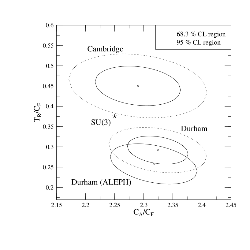
FIG. 5.: Confidence level contours of the leading order fits of the color charges $x$ and $y$ for the Durham and Cambridge clustering at $y_{\rm cut}=0.008$.

One may ask how the light gluino exclusion significance changes in the recent analysis of Csikor and Fodor [22], which used the results of four-jet analyses, if one takes into account the systematic theoretical error discussed above. Assuming that the shifts of $x$ and $y$ are similar in the light gluino extension of QCD, our conclusion suggests that the radiative corrections induce a shift of order $2\alpha_{s}$ times the tree-level value for $x$ and $y$. Lacking this piece of information Csikor and Fodor have increased the axes of the error ellipses by a factor of ${\alpha_{s}}$ times the theoretical $x$ and $y$ values. Implementing our results to a Csikor-Fodor type analysis for the four-jet events would decrease their confidence levels for the light gluino exclusion from 99.9 % (Csikor-Fodor value) to $\simeq$98 %, which is, however, still much higher than a 2-$\sigma$ exclusion.

V Conclusion

In this paper we presented the next-to-leading order corrections to the group independent kinematical functions of the four standard four-jet angular distributions, $\cos\phi_{{\rm KSW}}$, $|\cos\theta^{*}_{{\rm NR}}|$, $\cos\alpha_{{\rm 34}}$, and $|\cos\chi_{{\rm BZ}}|$ with jets defined with two — the Durham and the Cambridge — clustering algorithms at $y_{\rm cut}=0.008$. These results were obtained with a general purpose Monte Carlo program called DEBRECEN [23] that can be used to calculate the differential distribution of any other four-jet quantity at the next-to-leading order accuracy in electron-positron annihilation. The $|\cos\chi_{{\rm BZ}}|$ distribution using the Durham clustering algorithm was first calculated by Signer [10]. Our result agrees with his within statistical errors. The results for the other three distributions with Durham clustering as well as for all distributions when the Cambridge algorithm is used are new. We compared our results to data obtained by the ALEPH collaboration corrected to parton level and found very good qualitative agreement. We have also presented the $K$ factors of the distributions using both jet clustering algorithms.

Having the next-to-leading order perturbative QCD prediction at our disposal we made an estimate of the systematic theoretical error of the QCD color charge measurements due to the use of leading order group independent kinematical functions. We found that the use of the O($\alpha_{s}^{3}$) QCD predictions instead of the O($\alpha_{s}^{2}$) results may shift the center of the fit by a relative factor of about $1+2{\alpha_{s}}$ in the $T_{R}/C_{F}$ direction, while the best $C_{A}/C_{F}$ value is hardly affected.

We are grateful to F. Csikor, Z. Fodor and S. Catani for useful communication, and to G. Dissertori for providing us the ALEPH data. This research was supported in part by the EEC Programme ”Human Capital and Mobility”, Network ”Physics at High Energy Colliders”, contract PECO ERBCIPDCT 94 0613 as well as by the Hungarian Scientific Research Fund grant OTKA T-016613 and the Research Group in Physics of the Hungarian Academy of Sciences, Debrecen.

VI Appendix

TABLE III.: Next-to-leading order kinematical functions to the $\cos\phi_{{\rm KSW}}$ angular distribution. The Durham jet algorithm is used.

$\cos\phi_{{\rm KSW}}$	$C_{4}\quad$	$C_{0}\quad$	$C_{x}\quad$	$C_{y}\quad$	$C_{xx}\quad$	$C_{xy}\quad$	$C_{yy}\quad$
-0.950	$\!\!1190.6\pm 25.0\!\!$	$\!\!-159.3\pm 6.7\!\!$	$\!\!655.2\pm 8.9\!\!$	$\!\!-1504.8\pm 11.8\!\!$	$\!\!129.7\pm 3.6\!\!$	$\!\!-235.6\pm 5.2\!\!$	$\!\!-128.0\pm 0.7\!\!$
-0.850	$\!\!686.5\pm 21.2\!\!$	$\!\!-86.7\pm 5.8\!\!$	$\!\!381.8\pm 7.6\!\!$	$\!\!-889.8\pm 9.3\!\!$	$\!\!70.7\pm 2.9\!\!$	$\!\!-109.6\pm 3.8\!\!$	$\!\!-127.9\pm 1.0\!\!$
-0.750	$\!\!696.9\pm 19.4\!\!$	$\!\!-67.5\pm 5.1\!\!$	$\!\!353.1\pm 7.2\!\!$	$\!\!-826.6\pm 9.8\!\!$	$\!\!73.3\pm 2.8\!\!$	$\!\!-82.4\pm 3.6\!\!$	$\!\!-157.4\pm 1.4\!\!$
-0.650	$\!\!707.5\pm 22.6\!\!$	$\!\!-73.8\pm 5.3\!\!$	$\!\!352.2\pm 7.8\!\!$	$\!\!-822.8\pm 9.7\!\!$	$\!\!73.9\pm 3.0\!\!$	$\!\!-61.5\pm 3.8\!\!$	$\!\!-179.4\pm 1.7\!\!$
-0.550	$\!\!722.0\pm 20.9\!\!$	$\!\!-73.7\pm 5.0\!\!$	$\!\!366.5\pm 8.1\!\!$	$\!\!-851.9\pm 9.9\!\!$	$\!\!70.9\pm 2.7\!\!$	$\!\!-48.2\pm 3.9\!\!$	$\!\!-196.7\pm 1.8\!\!$
-0.450	$\!\!716.2\pm 19.7\!\!$	$\!\!-77.9\pm 5.2\!\!$	$\!\!373.9\pm 8.2\!\!$	$\!\!-881.7\pm 11.0\!\!$	$\!\!67.0\pm 2.4\!\!$	$\!\!-32.6\pm 3.9\!\!$	$\!\!-203.8\pm 2.1\!\!$
-0.350	$\!\!708.5\pm 19.6\!\!$	$\!\!-87.8\pm 5.9\!\!$	$\!\!390.4\pm 7.9\!\!$	$\!\!-893.5\pm 10.4\!\!$	$\!\!57.8\pm 2.3\!\!$	$\!\!-10.3\pm 3.5\!\!$	$\!\!-206.5\pm 2.0\!\!$
-0.250	$\!\!763.1\pm 20.6\!\!$	$\!\!-78.2\pm 6.5\!\!$	$\!\!418.1\pm 9.2\!\!$	$\!\!-959.0\pm 11.7\!\!$	$\!\!57.5\pm 2.4\!\!$	$\!\!-2.0\pm 3.3\!\!$	$\!\!-207.1\pm 1.9\!\!$
-0.150	$\!\!752.5\pm 19.7\!\!$	$\!\!-77.7\pm 14.0\!\!$	$\!\!435.4\pm 10.6\!\!$	$\!\!-982.8\pm 11.7\!\!$	$\!\!46.9\pm 2.2\!\!$	$\!\!10.4\pm 3.0\!\!$	$\!\!-197.2\pm 1.8\!\!$
-0.050	$\!\!730.7\pm 18.8\!\!$	$\!\!-104.0\pm 7.3\!\!$	$\!\!457.3\pm 9.7\!\!$	$\!\!-1039.0\pm 12.7\!\!$	$\!\!41.1\pm 2.1\!\!$	$\!\!16.1\pm 2.6\!\!$	$\!\!-191.6\pm 2.0\!\!$
0.050	$\!\!665.5\pm 18.7\!\!$	$\!\!-90.7\pm 7.3\!\!$	$\!\!420.7\pm 9.9\!\!$	$\!\!-934.2\pm 12.6\!\!$	$\!\!31.6\pm 2.1\!\!$	$\!\!30.0\pm 2.5\!\!$	$\!\!-176.1\pm 1.8\!\!$
0.150	$\!\!652.9\pm 18.0\!\!$	$\!\!-84.7\pm 7.2\!\!$	$\!\!431.0\pm 9.6\!\!$	$\!\!-935.4\pm 13.3\!\!$	$\!\!21.2\pm 2.1\!\!$	$\!\!40.6\pm 2.6\!\!$	$\!\!-157.4\pm 1.5\!\!$
0.250	$\!\!631.6\pm 17.0\!\!$	$\!\!-86.2\pm 7.5\!\!$	$\!\!424.2\pm 9.8\!\!$	$\!\!-904.9\pm 13.4\!\!$	$\!\!17.5\pm 2.1\!\!$	$\!\!40.2\pm 2.1\!\!$	$\!\!-147.9\pm 1.4\!\!$
0.350	$\!\!633.7\pm 15.6\!\!$	$\!\!-83.3\pm 6.7\!\!$	$\!\!433.1\pm 9.5\!\!$	$\!\!-929.5\pm 13.4\!\!$	$\!\!14.5\pm 2.2\!\!$	$\!\!44.2\pm 2.2\!\!$	$\!\!-137.6\pm 1.3\!\!$
0.450	$\!\!576.9\pm 29.9\!\!$	$\!\!-105.1\pm 7.3\!\!$	$\!\!404.6\pm 42.6\!\!$	$\!\!-923.4\pm 12.7\!\!$	$\!\!18.9\pm 13.3\!\!$	$\!\!47.5\pm 2.2\!\!$	$\!\!-127.2\pm 1.2\!\!$
0.550	$\!\!628.8\pm 29.5\!\!$	$\!\!-100.3\pm 8.5\!\!$	$\!\!484.4\pm 42.6\!\!$	$\!\!-980.6\pm 13.5\!\!$	$\!\!-4.0\pm 13.5\!\!$	$\!\!52.6\pm 2.6\!\!$	$\!\!-122.8\pm 1.1\!\!$
0.650	$\!\!628.4\pm 16.2\!\!$	$\!\!-114.0\pm 8.7\!\!$	$\!\!483.6\pm 12.3\!\!$	$\!\!-1041.5\pm 14.2\!\!$	$\!\!2.3\pm 3.3\!\!$	$\!\!59.3\pm 2.9\!\!$	$\!\!-119.7\pm 1.0\!\!$
0.750	$\!\!711.1\pm 15.9\!\!$	$\!\!-132.8\pm 9.8\!\!$	$\!\!578.1\pm 13.9\!\!$	$\!\!-1197.2\pm 15.5\!\!$	$\!\!-9.8\pm 3.7\!\!$	$\!\!68.2\pm 3.1\!\!$	$\!\!-118.2\pm 0.9\!\!$
0.850	$\!\!836.8\pm 15.6\!\!$	$\!\!-169.5\pm 10.8\!\!$	$\!\!675.8\pm 14.2\!\!$	$\!\!-1444.1\pm 17.4\!\!$	$\!\!-3.3\pm 4.1\!\!$	$\!\!74.0\pm 3.7\!\!$	$\!\!-130.3\pm 1.1\!\!$
0.950	$\!\!1820.0\pm 22.9\!\!$	$\!\!-399.8\pm 12.9\!\!$	$\!\!1547.2\pm 16.8\!\!$	$\!\!-3258.7\pm 23.5\!\!$	$\!\!-29.1\pm 4.8\!\!$	$\!\!168.9\pm 5.1\!\!$	$\!\!-252.6\pm 1.3\!\!$

TABLE IV.: Next-to-leading order kinematical functions to the $|\cos\theta^{*}_{{\rm NR}}|$ angular distribution. The Durham jet algorithm is used.

$|\cos\theta^{*}_{{\rm NR}}|$	$C_{4}\quad$	$C_{0}\quad$	$C_{x}\quad$	$C_{y}\quad$	$C_{xx}\quad$	$C_{xy}\quad$	$C_{yy}\quad$
0.025	$\!\!1184.8\pm 26.6\!\!$	$\!\!-164.6\pm 10.5\!\!$	$\!\!757.6\pm 16.8\!\!$	$\!\!-1769.9\pm 24.6\!\!$	$\!\!46.2\pm 5.5\!\!$	$\!\!161.7\pm 7.8\!\!$	$\!\!-459.4\pm 4.3\!\!$
0.075	$\!\!1130.0\pm 35.3\!\!$	$\!\!-170.6\pm 12.3\!\!$	$\!\!757.8\pm 21.3\!\!$	$\!\!-1755.2\pm 26.9\!\!$	$\!\!36.7\pm 6.7\!\!$	$\!\!156.8\pm 8.6\!\!$	$\!\!-450.0\pm 4.4\!\!$
0.125	$\!\!1204.4\pm 37.0\!\!$	$\!\!-164.8\pm 12.0\!\!$	$\!\!780.8\pm 22.2\!\!$	$\!\!-1783.0\pm 25.5\!\!$	$\!\!43.0\pm 7.1\!\!$	$\!\!150.8\pm 8.2\!\!$	$\!\!-451.7\pm 4.1\!\!$
0.175	$\!\!1190.0\pm 39.9\!\!$	$\!\!-170.9\pm 14.7\!\!$	$\!\!764.6\pm 20.2\!\!$	$\!\!-1813.6\pm 28.1\!\!$	$\!\!52.0\pm 6.6\!\!$	$\!\!142.6\pm 8.5\!\!$	$\!\!-451.4\pm 4.1\!\!$
0.225	$\!\!1239.0\pm 37.9\!\!$	$\!\!-172.1\pm 13.9\!\!$	$\!\!801.1\pm 18.7\!\!$	$\!\!-1828.6\pm 28.7\!\!$	$\!\!47.1\pm 5.9\!\!$	$\!\!139.5\pm 7.5\!\!$	$\!\!-432.3\pm 4.0\!\!$
0.275	$\!\!1247.5\pm 32.2\!\!$	$\!\!-172.4\pm 12.4\!\!$	$\!\!796.1\pm 18.3\!\!$	$\!\!-1832.1\pm 25.7\!\!$	$\!\!54.2\pm 5.8\!\!$	$\!\!115.2\pm 8.0\!\!$	$\!\!-423.6\pm 4.0\!\!$
0.325	$\!\!1268.2\pm 33.5\!\!$	$\!\!-189.6\pm 15.3\!\!$	$\!\!828.9\pm 19.7\!\!$	$\!\!-1885.8\pm 25.7\!\!$	$\!\!54.7\pm 6.4\!\!$	$\!\!100.1\pm 8.5\!\!$	$\!\!-408.9\pm 3.5\!\!$
0.375	$\!\!1311.9\pm 40.1\!\!$	$\!\!-187.4\pm 14.6\!\!$	$\!\!824.8\pm 20.1\!\!$	$\!\!-1903.0\pm 26.0\!\!$	$\!\!68.5\pm 6.3\!\!$	$\!\!74.3\pm 7.7\!\!$	$\!\!-386.8\pm 3.2\!\!$
0.425	$\!\!1358.3\pm 41.6\!\!$	$\!\!-177.3\pm 13.0\!\!$	$\!\!888.3\pm 20.6\!\!$	$\!\!-1986.6\pm 26.8\!\!$	$\!\!56.5\pm 6.3\!\!$	$\!\!55.9\pm 7.4\!\!$	$\!\!-374.3\pm 3.2\!\!$
0.475	$\!\!1456.3\pm 38.0\!\!$	$\!\!-201.0\pm 13.5\!\!$	$\!\!916.8\pm 20.5\!\!$	$\!\!-2044.7\pm 27.4\!\!$	$\!\!74.9\pm 5.9\!\!$	$\!\!38.5\pm 7.4\!\!$	$\!\!-356.7\pm 3.0\!\!$
0.525	$\!\!1443.4\pm 41.3\!\!$	$\!\!-225.8\pm 14.3\!\!$	$\!\!951.0\pm 20.6\!\!$	$\!\!-2130.4\pm 26.3\!\!$	$\!\!69.0\pm 5.8\!\!$	$\!\!34.1\pm 6.9\!\!$	$\!\!-342.0\pm 3.1\!\!$
0.575	$\!\!1570.0\pm 60.5\!\!$	$\!\!-208.6\pm 14.3\!\!$	$\!\!980.2\pm 29.9\!\!$	$\!\!-2198.9\pm 26.5\!\!$	$\!\!89.4\pm 6.3\!\!$	$\!\!-11.4\pm 7.2\!\!$	$\!\!-317.0\pm 2.5\!\!$
0.625	$\!\!1662.7\pm 59.7\!\!$	$\!\!-249.2\pm 14.6\!\!$	$\!\!1085.3\pm 28.5\!\!$	$\!\!-2305.5\pm 26.3\!\!$	$\!\!79.1\pm 5.8\!\!$	$\!\!-30.2\pm 6.7\!\!$	$\!\!-300.8\pm 2.5\!\!$
0.675	$\!\!1806.9\pm 60.9\!\!$	$\!\!-233.2\pm 15.9\!\!$	$\!\!1146.4\pm 30.3\!\!$	$\!\!-2448.1\pm 31.4\!\!$	$\!\!92.6\pm 6.1\!\!$	$\!\!-61.2\pm 7.1\!\!$	$\!\!-276.8\pm 2.2\!\!$
0.725	$\!\!1689.3\pm 62.1\!\!$	$\!\!-279.2\pm 18.5\!\!$	$\!\!1129.5\pm 30.7\!\!$	$\!\!-2503.3\pm 30.8\!\!$	$\!\!93.3\pm 6.3\!\!$	$\!\!-83.3\pm 6.8\!\!$	$\!\!-249.5\pm 1.8\!\!$
0.775	$\!\!1913.3\pm 50.4\!\!$	$\!\!-263.6\pm 16.6\!\!$	$\!\!1244.8\pm 23.8\!\!$	$\!\!-2605.8\pm 29.0\!\!$	$\!\!93.6\pm 6.9\!\!$	$\!\!-105.4\pm 6.2\!\!$	$\!\!-226.0\pm 1.6\!\!$
0.825	$\!\!1931.5\pm 52.0\!\!$	$\!\!-290.4\pm 17.1\!\!$	$\!\!1269.4\pm 22.1\!\!$	$\!\!-2670.3\pm 28.0\!\!$	$\!\!101.2\pm 6.2\!\!$	$\!\!-139.6\pm 6.7\!\!$	$\!\!-200.1\pm 1.4\!\!$
0.875	$\!\!1907.6\pm 50.7\!\!$	$\!\!-284.7\pm 17.9\!\!$	$\!\!1254.5\pm 22.7\!\!$	$\!\!-2691.0\pm 30.5\!\!$	$\!\!106.3\pm 5.7\!\!$	$\!\!-160.8\pm 7.6\!\!$	$\!\!-173.4\pm 1.3\!\!$
0.925	$\!\!1979.0\pm 56.1\!\!$	$\!\!-302.0\pm 31.4\!\!$	$\!\!1297.6\pm 26.1\!\!$	$\!\!-2777.3\pm 29.1\!\!$	$\!\!116.5\pm 6.3\!\!$	$\!\!-196.4\pm 7.4\!\!$	$\!\!-151.9\pm 1.1\!\!$
0.975	$\!\!2426.4\pm 68.3\!\!$	$\!\!-399.1\pm 19.4\!\!$	$\!\!1658.0\pm 27.8\!\!$	$\!\!-3469.3\pm 33.7\!\!$	$\!\!122.2\pm 6.5\!\!$	$\!\!-241.3\pm 8.3\!\!$	$\!\!-137.8\pm 0.8\!\!$

TABLE V.: Next-to-leading order kinematical functions to the $\cos\alpha_{{\rm 34}}$ angular distribution. The Durham jet algorithm is used.

$\cos\alpha_{{\rm 34}}$	$C_{4}\quad$	$C_{0}\quad$	$C_{x}\quad$	$C_{y}\quad$	$C_{xx}\quad$	$C_{xy}\quad$	$C_{yy}\quad$
-0.950	$\!\!1038.4\pm 17.9\!\!$	$\!\!-227.3\pm 9.1\!\!$	$\!\!901.2\pm 12.1\!\!$	$\!\!-1888.6\pm 17.5\!\!$	$\!\!-20.6\pm 2.8\!\!$	$\!\!77.1\pm 2.9\!\!$	$\!\!-106.0\pm 0.8\!\!$
-0.850	$\!\!988.9\pm 19.5\!\!$	$\!\!-187.7\pm 9.0\!\!$	$\!\!830.9\pm 12.8\!\!$	$\!\!-1717.5\pm 17.9\!\!$	$\!\!-19.0\pm 3.0\!\!$	$\!\!73.8\pm 2.9\!\!$	$\!\!-109.0\pm 0.8\!\!$
-0.750	$\!\!948.7\pm 19.4\!\!$	$\!\!-177.0\pm 9.2\!\!$	$\!\!777.1\pm 13.9\!\!$	$\!\!-1628.8\pm 16.6\!\!$	$\!\!-10.4\pm 3.5\!\!$	$\!\!67.2\pm 2.7\!\!$	$\!\!-116.9\pm 0.9\!\!$
-0.650	$\!\!911.1\pm 22.2\!\!$	$\!\!-162.4\pm 9.6\!\!$	$\!\!716.5\pm 13.0\!\!$	$\!\!-1500.5\pm 15.4\!\!$	$\!\!-0.9\pm 2.9\!\!$	$\!\!54.8\pm 2.7\!\!$	$\!\!-123.8\pm 1.0\!\!$
-0.550	$\!\!899.6\pm 26.1\!\!$	$\!\!-144.1\pm 7.9\!\!$	$\!\!684.6\pm 14.7\!\!$	$\!\!-1427.9\pm 15.6\!\!$	$\!\!3.4\pm 3.1\!\!$	$\!\!47.9\pm 2.7\!\!$	$\!\!-132.5\pm 1.0\!\!$
-0.450	$\!\!849.9\pm 22.1\!\!$	$\!\!-131.0\pm 15.0\!\!$	$\!\!629.7\pm 14.3\!\!$	$\!\!-1381.1\pm 15.8\!\!$	$\!\!12.9\pm 3.4\!\!$	$\!\!43.0\pm 3.0\!\!$	$\!\!-141.0\pm 1.1\!\!$
-0.350	$\!\!827.5\pm 21.1\!\!$	$\!\!-133.5\pm 7.3\!\!$	$\!\!597.8\pm 11.5\!\!$	$\!\!-1268.9\pm 15.7\!\!$	$\!\!16.0\pm 3.2\!\!$	$\!\!38.1\pm 2.9\!\!$	$\!\!-148.8\pm 1.2\!\!$
-0.250	$\!\!816.0\pm 19.0\!\!$	$\!\!-126.8\pm 6.8\!\!$	$\!\!566.3\pm 11.6\!\!$	$\!\!-1235.8\pm 14.7\!\!$	$\!\!25.9\pm 2.9\!\!$	$\!\!26.5\pm 2.8\!\!$	$\!\!-158.2\pm 1.2\!\!$
-0.150	$\!\!810.4\pm 19.8\!\!$	$\!\!-125.3\pm 7.0\!\!$	$\!\!546.5\pm 12.2\!\!$	$\!\!-1200.7\pm 14.2\!\!$	$\!\!32.2\pm 3.6\!\!$	$\!\!20.0\pm 3.2\!\!$	$\!\!-171.5\pm 1.3\!\!$
-0.050	$\!\!843.6\pm 21.4\!\!$	$\!\!-118.9\pm 7.4\!\!$	$\!\!534.6\pm 13.5\!\!$	$\!\!-1187.5\pm 14.9\!\!$	$\!\!44.4\pm 3.9\!\!$	$\!\!7.4\pm 3.2\!\!$	$\!\!-187.6\pm 1.5\!\!$
0.050	$\!\!829.9\pm 21.7\!\!$	$\!\!-126.0\pm 6.7\!\!$	$\!\!510.9\pm 10.3\!\!$	$\!\!-1152.5\pm 13.3\!\!$	$\!\!53.0\pm 2.7\!\!$	$\!\!-1.4\pm 3.4\!\!$	$\!\!-203.9\pm 1.6\!\!$
0.150	$\!\!879.4\pm 23.4\!\!$	$\!\!-105.2\pm 7.2\!\!$	$\!\!484.1\pm 10.1\!\!$	$\!\!-1100.1\pm 13.4\!\!$	$\!\!69.4\pm 2.9\!\!$	$\!\!-14.5\pm 3.9\!\!$	$\!\!-219.1\pm 1.8\!\!$
0.250	$\!\!834.2\pm 21.6\!\!$	$\!\!-104.4\pm 6.2\!\!$	$\!\!450.9\pm 8.9\!\!$	$\!\!-1055.2\pm 12.4\!\!$	$\!\!74.0\pm 2.7\!\!$	$\!\!-28.7\pm 4.2\!\!$	$\!\!-233.1\pm 2.1\!\!$
0.350	$\!\!837.2\pm 23.9\!\!$	$\!\!-93.4\pm 5.6\!\!$	$\!\!426.1\pm 8.7\!\!$	$\!\!-999.6\pm 11.9\!\!$	$\!\!83.0\pm 3.1\!\!$	$\!\!-43.0\pm 4.5\!\!$	$\!\!-244.0\pm 2.0\!\!$
0.450	$\!\!828.0\pm 24.0\!\!$	$\!\!-79.6\pm 5.3\!\!$	$\!\!382.7\pm 7.8\!\!$	$\!\!-915.3\pm 11.1\!\!$	$\!\!93.2\pm 3.4\!\!$	$\!\!-55.2\pm 4.9\!\!$	$\!\!-249.9\pm 2.1\!\!$
0.550	$\!\!793.7\pm 22.2\!\!$	$\!\!-72.9\pm 4.5\!\!$	$\!\!343.9\pm 8.9\!\!$	$\!\!-854.5\pm 10.3\!\!$	$\!\!100.1\pm 2.7\!\!$	$\!\!-70.2\pm 5.0\!\!$	$\!\!-252.9\pm 2.1\!\!$
0.650	$\!\!719.8\pm 21.9\!\!$	$\!\!-59.1\pm 5.0\!\!$	$\!\!305.2\pm 8.4\!\!$	$\!\!-763.9\pm 8.4\!\!$	$\!\!94.0\pm 2.9\!\!$	$\!\!-74.7\pm 5.0\!\!$	$\!\!-238.4\pm 2.1\!\!$
0.750	$\!\!546.0\pm 15.0\!\!$	$\!\!-52.5\pm 4.1\!\!$	$\!\!238.4\pm 5.2\!\!$	$\!\!-602.4\pm 7.5\!\!$	$\!\!73.0\pm 2.5\!\!$	$\!\!-66.1\pm 4.0\!\!$	$\!\!-184.8\pm 2.1\!\!$
0.850	$\!\!245.2\pm 9.3\!\!$	$\!\!-24.0\pm 2.9\!\!$	$\!\!130.1\pm 3.4\!\!$	$\!\!-302.8\pm 5.2\!\!$	$\!\!24.8\pm 1.7\!\!$	$\!\!-31.7\pm 2.4\!\!$	$\!\!-62.8\pm 0.9\!\!$
0.950	$\!\!12.5\pm 2.4\!\!$	$\!\!-1.9\pm 1.0\!\!$	$\!\!9.2\pm 1.3\!\!$	$\!\!-17.7\pm 1.4\!\!$	$\!\!0.2\pm 0.2\!\!$	$\!\!-0.4\pm 0.2\!\!$	$\!\!-0.9\pm 0.1\!\!$

TABLE VI.: Next-to-leading order kinematical functions to the $|\cos\chi_{{\rm BZ}}|$ angular distribution. The Durham jet algorithm is used.

$|\cos\chi_{{\rm BZ}}|$	$C_{4}\quad$	$C_{0}\quad$	$C_{x}\quad$	$C_{y}\quad$	$C_{xx}\quad$	$C_{xy}\quad$	$C_{yy}\quad$
0.025	$\!\!1133.9\pm 39.7\!\!$	$\!\!-171.8\pm 14.1\!\!$	$\!\!748.6\pm 24.7\!\!$	$\!\!-1623.5\pm 30.9\!\!$	$\!\!29.2\pm 6.3\!\!$	$\!\!161.8\pm 8.2\!\!$	$\!\!-400.9\pm 4.4\!\!$
0.075	$\!\!1087.1\pm 47.9\!\!$	$\!\!-170.2\pm 17.3\!\!$	$\!\!724.3\pm 35.3\!\!$	$\!\!-1689.3\pm 31.6\!\!$	$\!\!34.9\pm 9.9\!\!$	$\!\!164.9\pm 9.2\!\!$	$\!\!-395.9\pm 4.2\!\!$
0.125	$\!\!1147.7\pm 49.5\!\!$	$\!\!-163.0\pm 18.2\!\!$	$\!\!771.0\pm 35.7\!\!$	$\!\!-1640.7\pm 26.6\!\!$	$\!\!23.1\pm 11.0\!\!$	$\!\!153.2\pm 7.8\!\!$	$\!\!-395.1\pm 4.1\!\!$
0.175	$\!\!1075.4\pm 45.9\!\!$	$\!\!-160.2\pm 16.6\!\!$	$\!\!719.1\pm 27.9\!\!$	$\!\!-1665.6\pm 26.8\!\!$	$\!\!33.6\pm 8.9\!\!$	$\!\!159.0\pm 9.3\!\!$	$\!\!-391.4\pm 4.2\!\!$
0.225	$\!\!1144.5\pm 42.5\!\!$	$\!\!-177.8\pm 16.9\!\!$	$\!\!752.8\pm 27.3\!\!$	$\!\!-1659.9\pm 25.7\!\!$	$\!\!36.9\pm 7.5\!\!$	$\!\!135.4\pm 8.9\!\!$	$\!\!-381.4\pm 3.9\!\!$
0.275	$\!\!1110.3\pm 43.5\!\!$	$\!\!-172.6\pm 17.9\!\!$	$\!\!741.9\pm 29.0\!\!$	$\!\!-1634.2\pm 27.2\!\!$	$\!\!33.4\pm 8.2\!\!$	$\!\!121.7\pm 8.1\!\!$	$\!\!-361.1\pm 3.7\!\!$
0.325	$\!\!1152.2\pm 42.3\!\!$	$\!\!-142.2\pm 18.6\!\!$	$\!\!744.5\pm 28.2\!\!$	$\!\!-1651.3\pm 26.3\!\!$	$\!\!39.0\pm 7.8\!\!$	$\!\!110.2\pm 7.7\!\!$	$\!\!-350.3\pm 3.1\!\!$
0.375	$\!\!1181.2\pm 43.1\!\!$	$\!\!-175.4\pm 16.9\!\!$	$\!\!794.6\pm 28.2\!\!$	$\!\!-1741.2\pm 26.3\!\!$	$\!\!35.9\pm 7.3\!\!$	$\!\!106.1\pm 6.8\!\!$	$\!\!-340.5\pm 3.3\!\!$
0.425	$\!\!1210.8\pm 47.8\!\!$	$\!\!-155.7\pm 16.7\!\!$	$\!\!798.5\pm 36.3\!\!$	$\!\!-1693.3\pm 26.2\!\!$	$\!\!37.9\pm 10.1\!\!$	$\!\!72.5\pm 7.5\!\!$	$\!\!-330.6\pm 3.2\!\!$
0.475	$\!\!1213.1\pm 44.5\!\!$	$\!\!-185.8\pm 17.7\!\!$	$\!\!762.7\pm 34.5\!\!$	$\!\!-1749.9\pm 25.3\!\!$	$\!\!66.2\pm 9.4\!\!$	$\!\!56.7\pm 7.7\!\!$	$\!\!-322.3\pm 2.9\!\!$
0.525	$\!\!1236.6\pm 38.9\!\!$	$\!\!-195.1\pm 18.2\!\!$	$\!\!819.6\pm 24.7\!\!$	$\!\!-1801.7\pm 23.2\!\!$	$\!\!53.0\pm 6.6\!\!$	$\!\!44.5\pm 6.3\!\!$	$\!\!-310.7\pm 2.8\!\!$
0.575	$\!\!1337.2\pm 42.9\!\!$	$\!\!-182.4\pm 18.0\!\!$	$\!\!847.8\pm 24.9\!\!$	$\!\!-1855.7\pm 24.3\!\!$	$\!\!65.6\pm 6.7\!\!$	$\!\!19.1\pm 5.8\!\!$	$\!\!-299.8\pm 2.5\!\!$
0.625	$\!\!1383.5\pm 44.4\!\!$	$\!\!-201.5\pm 16.0\!\!$	$\!\!891.7\pm 23.7\!\!$	$\!\!-1983.3\pm 24.3\!\!$	$\!\!72.4\pm 6.5\!\!$	$\!\!-2.5\pm 5.8\!\!$	$\!\!-292.6\pm 2.3\!\!$
0.675	$\!\!1415.8\pm 44.2\!\!$	$\!\!-197.9\pm 15.9\!\!$	$\!\!916.5\pm 24.2\!\!$	$\!\!-2050.8\pm 25.1\!\!$	$\!\!74.8\pm 6.4\!\!$	$\!\!-22.5\pm 6.1\!\!$	$\!\!-279.9\pm 2.0\!\!$
0.725	$\!\!1551.9\pm 44.0\!\!$	$\!\!-283.2\pm 89.5\!\!$	$\!\!1039.4\pm 77.4\!\!$	$\!\!-2150.5\pm 25.3\!\!$	$\!\!74.9\pm 15.7\!\!$	$\!\!-45.4\pm 6.4\!\!$	$\!\!-268.6\pm 2.0\!\!$
0.775	$\!\!1659.4\pm 47.8\!\!$	$\!\!-152.9\pm 90.5\!\!$	$\!\!1020.2\pm 77.7\!\!$	$\!\!-2357.4\pm 26.3\!\!$	$\!\!99.2\pm 15.8\!\!$	$\!\!-75.9\pm 6.7\!\!$	$\!\!-262.1\pm 1.9\!\!$
0.825	$\!\!1828.2\pm 48.2\!\!$	$\!\!-251.4\pm 17.7\!\!$	$\!\!1166.8\pm 26.1\!\!$	$\!\!-2553.8\pm 25.9\!\!$	$\!\!105.5\pm 6.3\!\!$	$\!\!-102.4\pm 7.0\!\!$	$\!\!-248.7\pm 1.6\!\!$
0.875	$\!\!1791.5\pm 245.1\!\!$	$\!\!-316.9\pm 32.0\!\!$	$\!\!1236.4\pm 91.5\!\!$	$\!\!-2863.7\pm 27.2\!\!$	$\!\!110.1\pm 8.8\!\!$	$\!\!-146.7\pm 7.0\!\!$	$\!\!-243.1\pm 1.6\!\!$
0.925	$\!\!2455.5\pm 246.3\!\!$	$\!\!-318.9\pm 33.3\!\!$	$\!\!1528.1\pm 91.8\!\!$	$\!\!-3230.3\pm 28.2\!\!$	$\!\!151.2\pm 9.1\!\!$	$\!\!-217.0\pm 7.9\!\!$	$\!\!-249.3\pm 1.5\!\!$
0.975	$\!\!4804.5\pm 70.2\!\!$	$\!\!-731.4\pm 36.2\!\!$	$\!\!3109.1\pm 34.0\!\!$	$\!\!-6806.4\pm 41.7\!\!$	$\!\!320.2\pm 8.8\!\!$	$\!\!-552.9\pm 12.4\!\!$	$\!\!-445.9\pm 1.9\!\!$

TABLE VII.: Next-to-leading order kinematical functions to the $\cos\phi_{{\rm KSW}}$ angular distribution. The Cambridge jet algorithm is used.

$\cos\phi_{{\rm KSW}}$	$C_{4}\quad$	$C_{0}\quad$	$C_{x}\quad$	$C_{y}\quad$	$C_{xx}\quad$	$C_{xy}\quad$	$C_{yy}\quad$
-0.950	$\!\!1085.9\pm 44.0\!\!$	$\!\!-287.0\pm 8.1\!\!$	$\!\!713.0\pm 12.8\!\!$	$\!\!-1754.9\pm 17.4\!\!$	$\!\!135.1\pm 7.2\!\!$	$\!\!-280.6\pm 8.0\!\!$	$\!\!-143.7\pm 0.9\!\!$
-0.850	$\!\!658.4\pm 35.4\!\!$	$\!\!-164.3\pm 7.1\!\!$	$\!\!404.4\pm 10.0\!\!$	$\!\!-986.2\pm 12.6\!\!$	$\!\!81.7\pm 4.9\!\!$	$\!\!-134.9\pm 6.1\!\!$	$\!\!-134.0\pm 1.2\!\!$
-0.750	$\!\!617.4\pm 27.0\!\!$	$\!\!-139.8\pm 8.8\!\!$	$\!\!366.6\pm 9.6\!\!$	$\!\!-932.2\pm 13.9\!\!$	$\!\!78.5\pm 3.7\!\!$	$\!\!-108.1\pm 6.0\!\!$	$\!\!-170.1\pm 1.6\!\!$
-0.650	$\!\!620.0\pm 23.2\!\!$	$\!\!-124.2\pm 8.8\!\!$	$\!\!355.9\pm 9.5\!\!$	$\!\!-924.0\pm 14.5\!\!$	$\!\!74.7\pm 3.1\!\!$	$\!\!-71.1\pm 5.7\!\!$	$\!\!-196.1\pm 2.0\!\!$
-0.550	$\!\!662.8\pm 23.0\!\!$	$\!\!-130.5\pm 7.9\!\!$	$\!\!377.7\pm 10.5\!\!$	$\!\!-961.9\pm 13.0\!\!$	$\!\!75.7\pm 3.2\!\!$	$\!\!-59.5\pm 4.6\!\!$	$\!\!-210.4\pm 2.2\!\!$
-0.450	$\!\!605.2\pm 24.4\!\!$	$\!\!-145.8\pm 8.2\!\!$	$\!\!380.8\pm 10.6\!\!$	$\!\!-954.7\pm 13.1\!\!$	$\!\!60.8\pm 3.0\!\!$	$\!\!-30.6\pm 4.4\!\!$	$\!\!-216.4\pm 2.5\!\!$
-0.350	$\!\!658.4\pm 23.8\!\!$	$\!\!-143.1\pm 7.8\!\!$	$\!\!405.4\pm 10.4\!\!$	$\!\!-1004.1\pm 14.8\!\!$	$\!\!60.9\pm 2.7\!\!$	$\!\!-13.3\pm 4.4\!\!$	$\!\!-224.1\pm 2.7\!\!$
-0.250	$\!\!653.0\pm 25.4\!\!$	$\!\!-148.1\pm 7.6\!\!$	$\!\!421.2\pm 11.6\!\!$	$\!\!-1035.8\pm 15.6\!\!$	$\!\!54.3\pm 2.6\!\!$	$\!\!-4.2\pm 4.6\!\!$	$\!\!-219.6\pm 2.5\!\!$
-0.150	$\!\!610.7\pm 25.0\!\!$	$\!\!-173.7\pm 8.8\!\!$	$\!\!431.9\pm 12.1\!\!$	$\!\!-1044.3\pm 16.1\!\!$	$\!\!44.3\pm 2.8\!\!$	$\!\!13.4\pm 4.3\!\!$	$\!\!-213.7\pm 2.4\!\!$
-0.050	$\!\!603.3\pm 23.6\!\!$	$\!\!-176.6\pm 12.3\!\!$	$\!\!449.2\pm 15.2\!\!$	$\!\!-1078.7\pm 16.5\!\!$	$\!\!36.9\pm 3.4\!\!$	$\!\!16.1\pm 3.8\!\!$	$\!\!-192.3\pm 2.2\!\!$
0.050	$\!\!548.4\pm 21.4\!\!$	$\!\!-147.6\pm 7.5\!\!$	$\!\!401.7\pm 10.6\!\!$	$\!\!-970.0\pm 14.6\!\!$	$\!\!30.8\pm 2.5\!\!$	$\!\!28.0\pm 2.6\!\!$	$\!\!-171.0\pm 2.0\!\!$
0.150	$\!\!514.7\pm 19.3\!\!$	$\!\!-161.5\pm 7.3\!\!$	$\!\!414.3\pm 10.2\!\!$	$\!\!-952.0\pm 13.2\!\!$	$\!\!18.2\pm 2.4\!\!$	$\!\!37.2\pm 2.9\!\!$	$\!\!-161.0\pm 1.8\!\!$
0.250	$\!\!508.4\pm 17.1\!\!$	$\!\!-153.8\pm 6.9\!\!$	$\!\!407.1\pm 10.0\!\!$	$\!\!-942.3\pm 12.7\!\!$	$\!\!17.3\pm 2.2\!\!$	$\!\!38.5\pm 2.9\!\!$	$\!\!-147.1\pm 1.6\!\!$
0.350	$\!\!500.3\pm 17.0\!\!$	$\!\!-158.0\pm 7.4\!\!$	$\!\!425.3\pm 13.3\!\!$	$\!\!-974.9\pm 14.6\!\!$	$\!\!9.9\pm 3.2\!\!$	$\!\!42.6\pm 2.2\!\!$	$\!\!-140.6\pm 1.5\!\!$
0.450	$\!\!497.7\pm 18.5\!\!$	$\!\!-164.4\pm 7.5\!\!$	$\!\!429.0\pm 13.9\!\!$	$\!\!-996.6\pm 13.9\!\!$	$\!\!10.0\pm 3.4\!\!$	$\!\!44.7\pm 2.4\!\!$	$\!\!-129.7\pm 1.3\!\!$
0.550	$\!\!471.1\pm 16.9\!\!$	$\!\!-177.1\pm 7.9\!\!$	$\!\!444.7\pm 12.0\!\!$	$\!\!-1027.1\pm 15.3\!\!$	$\!\!1.1\pm 2.9\!\!$	$\!\!52.3\pm 2.7\!\!$	$\!\!-124.8\pm 1.3\!\!$
0.650	$\!\!510.0\pm 16.8\!\!$	$\!\!-195.1\pm 7.8\!\!$	$\!\!489.6\pm 11.6\!\!$	$\!\!-1085.2\pm 15.0\!\!$	$\!\!-4.2\pm 3.1\!\!$	$\!\!56.5\pm 2.9\!\!$	$\!\!-120.9\pm 1.2\!\!$
0.750	$\!\!560.0\pm 17.4\!\!$	$\!\!-207.1\pm 8.3\!\!$	$\!\!545.7\pm 12.3\!\!$	$\!\!-1217.8\pm 15.2\!\!$	$\!\!-8.4\pm 3.2\!\!$	$\!\!65.2\pm 3.4\!\!$	$\!\!-118.7\pm 1.0\!\!$
0.850	$\!\!681.4\pm 22.0\!\!$	$\!\!-264.5\pm 9.5\!\!$	$\!\!687.5\pm 14.6\!\!$	$\!\!-1514.9\pm 18.8\!\!$	$\!\!-16.0\pm 3.7\!\!$	$\!\!78.5\pm 3.9\!\!$	$\!\!-129.7\pm 1.2\!\!$
0.950	$\!\!1493.1\pm 25.4\!\!$	$\!\!-630.2\pm 14.1\!\!$	$\!\!1574.3\pm 18.8\!\!$	$\!\!-3435.0\pm 24.6\!\!$	$\!\!-48.4\pm 5.7\!\!$	$\!\!176.7\pm 6.1\!\!$	$\!\!-252.8\pm 1.4\!\!$

TABLE VIII.: Next-to-leading order kinematical functions to the $|\cos\theta^{*}_{{\rm NR}}|$ angular distribution. The Cambridge jet algorithm is used.

$|\cos\theta^{*}_{{\rm NR}}|$	$C_{4}\quad$	$C_{0}\quad$	$C_{x}\quad$	$C_{y}\quad$	$C_{xx}\quad$	$C_{xy}\quad$	$C_{yy}\quad$
0.025	$\!\!1016.1\pm 30.2\!\!$	$\!\!-233.6\pm 14.4\!\!$	$\!\!750.2\pm 20.8\!\!$	$\!\!-1827.3\pm 28.5\!\!$	$\!\!34.8\pm 6.8\!\!$	$\!\!160.4\pm 9.5\!\!$	$\!\!-449.3\pm 4.6\!\!$
0.075	$\!\!1023.7\pm 38.2\!\!$	$\!\!-237.2\pm 12.6\!\!$	$\!\!734.5\pm 22.5\!\!$	$\!\!-1817.0\pm 32.1\!\!$	$\!\!46.1\pm 7.2\!\!$	$\!\!136.2\pm 10.2\!\!$	$\!\!-450.5\pm 4.6\!\!$
0.125	$\!\!1011.2\pm 44.1\!\!$	$\!\!-224.1\pm 13.7\!\!$	$\!\!756.4\pm 23.2\!\!$	$\!\!-1848.0\pm 30.1\!\!$	$\!\!31.7\pm 7.3\!\!$	$\!\!157.7\pm 9.7\!\!$	$\!\!-441.6\pm 5.0\!\!$
0.175	$\!\!1038.5\pm 44.3\!\!$	$\!\!-249.2\pm 13.3\!\!$	$\!\!760.8\pm 21.9\!\!$	$\!\!-1867.3\pm 27.9\!\!$	$\!\!44.8\pm 6.8\!\!$	$\!\!126.8\pm 10.1\!\!$	$\!\!-450.3\pm 4.5\!\!$
0.225	$\!\!1037.3\pm 42.3\!\!$	$\!\!-240.7\pm 11.0\!\!$	$\!\!760.2\pm 24.2\!\!$	$\!\!-1867.6\pm 29.5\!\!$	$\!\!43.9\pm 6.7\!\!$	$\!\!117.8\pm 11.4\!\!$	$\!\!-430.8\pm 4.0\!\!$
0.275	$\!\!1112.1\pm 42.0\!\!$	$\!\!-253.5\pm 12.1\!\!$	$\!\!807.4\pm 23.2\!\!$	$\!\!-1937.9\pm 27.2\!\!$	$\!\!47.7\pm 6.8\!\!$	$\!\!117.0\pm 11.3\!\!$	$\!\!-426.1\pm 4.6\!\!$
0.325	$\!\!1078.7\pm 37.7\!\!$	$\!\!-260.3\pm 13.6\!\!$	$\!\!808.9\pm 21.4\!\!$	$\!\!-1937.7\pm 27.0\!\!$	$\!\!44.1\pm 6.7\!\!$	$\!\!99.2\pm 9.0\!\!$	$\!\!-416.5\pm 4.0\!\!$
0.375	$\!\!1074.5\pm 37.2\!\!$	$\!\!-277.2\pm 13.6\!\!$	$\!\!797.5\pm 21.5\!\!$	$\!\!-1997.0\pm 29.2\!\!$	$\!\!57.6\pm 6.9\!\!$	$\!\!87.5\pm 10.1\!\!$	$\!\!-403.2\pm 3.8\!\!$
0.425	$\!\!1147.9\pm 39.6\!\!$	$\!\!-314.1\pm 15.2\!\!$	$\!\!896.8\pm 22.6\!\!$	$\!\!-2103.0\pm 28.6\!\!$	$\!\!46.6\pm 6.4\!\!$	$\!\!57.1\pm 10.0\!\!$	$\!\!-385.7\pm 3.7\!\!$
0.475	$\!\!1222.8\pm 43.0\!\!$	$\!\!-294.4\pm 13.3\!\!$	$\!\!911.7\pm 23.0\!\!$	$\!\!-2166.9\pm 30.0\!\!$	$\!\!58.9\pm 6.6\!\!$	$\!\!38.1\pm 7.9\!\!$	$\!\!-370.6\pm 3.9\!\!$
0.525	$\!\!1238.6\pm 46.5\!\!$	$\!\!-343.9\pm 15.0\!\!$	$\!\!944.9\pm 23.2\!\!$	$\!\!-2233.5\pm 27.5\!\!$	$\!\!62.5\pm 6.7\!\!$	$\!\!29.5\pm 8.0\!\!$	$\!\!-352.4\pm 3.7\!\!$
0.575	$\!\!1295.5\pm 45.3\!\!$	$\!\!-351.4\pm 15.1\!\!$	$\!\!969.0\pm 23.0\!\!$	$\!\!-2346.7\pm 30.8\!\!$	$\!\!78.8\pm 6.0\!\!$	$\!\!-4.6\pm 7.1\!\!$	$\!\!-334.3\pm 3.5\!\!$
0.625	$\!\!1371.8\pm 45.0\!\!$	$\!\!-393.9\pm 14.4\!\!$	$\!\!1069.7\pm 22.8\!\!$	$\!\!-2488.9\pm 31.3\!\!$	$\!\!72.3\pm 6.0\!\!$	$\!\!-39.0\pm 8.7\!\!$	$\!\!-315.0\pm 3.3\!\!$
0.675	$\!\!1403.5\pm 55.5\!\!$	$\!\!-452.3\pm 17.6\!\!$	$\!\!1134.1\pm 25.8\!\!$	$\!\!-2606.4\pm 34.4\!\!$	$\!\!75.7\pm 6.7\!\!$	$\!\!-73.7\pm 8.6\!\!$	$\!\!-294.4\pm 2.8\!\!$
0.725	$\!\!1504.7\pm 61.1\!\!$	$\!\!-455.9\pm 25.1\!\!$	$\!\!1183.5\pm 33.8\!\!$	$\!\!-2732.3\pm 34.7\!\!$	$\!\!85.6\pm 8.9\!\!$	$\!\!-86.4\pm 8.1\!\!$	$\!\!-274.2\pm 2.8\!\!$
0.775	$\!\!1479.6\pm 59.4\!\!$	$\!\!-539.4\pm 17.8\!\!$	$\!\!1202.1\pm 29.3\!\!$	$\!\!-2802.7\pm 33.0\!\!$	$\!\!99.7\pm 8.7\!\!$	$\!\!-126.3\pm 8.0\!\!$	$\!\!-250.6\pm 2.5\!\!$
0.825	$\!\!1527.5\pm 63.3\!\!$	$\!\!-566.6\pm 20.2\!\!$	$\!\!1268.4\pm 32.6\!\!$	$\!\!-2896.6\pm 34.1\!\!$	$\!\!94.9\pm 8.2\!\!$	$\!\!-142.1\pm 8.7\!\!$	$\!\!-230.8\pm 2.4\!\!$
0.875	$\!\!1585.8\pm 64.0\!\!$	$\!\!-629.1\pm 21.1\!\!$	$\!\!1318.0\pm 27.1\!\!$	$\!\!-2971.0\pm 34.6\!\!$	$\!\!110.0\pm 7.3\!\!$	$\!\!-196.0\pm 10.0\!\!$	$\!\!-204.7\pm 2.0\!\!$
0.925	$\!\!1706.3\pm 87.7\!\!$	$\!\!-625.3\pm 20.9\!\!$	$\!\!1357.8\pm 29.4\!\!$	$\!\!-3096.3\pm 37.4\!\!$	$\!\!130.8\pm 10.4\!\!$	$\!\!-234.3\pm 11.1\!\!$	$\!\!-180.9\pm 1.8\!\!$
0.975	$\!\!2243.9\pm 92.8\!\!$	$\!\!-842.0\pm 23.9\!\!$	$\!\!1818.8\pm 32.5\!\!$	$\!\!-4041.0\pm 44.8\!\!$	$\!\!160.3\pm 13.9\!\!$	$\!\!-329.7\pm 15.2\!\!$	$\!\!-171.8\pm 1.5\!\!$

TABLE IX.: Next-to-leading order kinematical functions to the $\cos\alpha_{{\rm 34}}$ angular distribution. The Cambridge jet algorithm is used.

$\cos\alpha_{{\rm 34}}$	$C_{4}\quad$	$C_{0}\quad$	$C_{x}\quad$	$C_{y}\quad$	$C_{xx}\quad$	$C_{xy}\quad$	$C_{yy}\quad$
-0.950	$\!\!827.2\pm 21.4\!\!$	$\!\!-373.0\pm 9.4\!\!$	$\!\!904.6\pm 13.6\!\!$	$\!\!-1956.5\pm 16.9\!\!$	$\!\!-30.4\pm 3.3\!\!$	$\!\!79.5\pm 3.1\!\!$	$\!\!-105.8\pm 0.9\!\!$
-0.850	$\!\!786.6\pm 41.6\!\!$	$\!\!-333.1\pm 10.3\!\!$	$\!\!819.7\pm 20.6\!\!$	$\!\!-1750.8\pm 19.7\!\!$	$\!\!-22.2\pm 3.0\!\!$	$\!\!70.2\pm 3.3\!\!$	$\!\!-108.9\pm 0.9\!\!$
-0.750	$\!\!731.5\pm 40.2\!\!$	$\!\!-310.3\pm 11.6\!\!$	$\!\!760.7\pm 19.6\!\!$	$\!\!-1686.0\pm 17.9\!\!$	$\!\!-15.0\pm 3.2\!\!$	$\!\!64.5\pm 3.2\!\!$	$\!\!-118.2\pm 1.0\!\!$
-0.650	$\!\!726.5\pm 21.4\!\!$	$\!\!-285.2\pm 10.0\!\!$	$\!\!718.2\pm 13.6\!\!$	$\!\!-1607.3\pm 18.0\!\!$	$\!\!-6.1\pm 3.2\!\!$	$\!\!56.4\pm 3.1\!\!$	$\!\!-126.8\pm 1.1\!\!$
-0.550	$\!\!691.0\pm 30.1\!\!$	$\!\!-257.9\pm 8.5\!\!$	$\!\!666.9\pm 15.9\!\!$	$\!\!-1473.9\pm 18.3\!\!$	$\!\!-4.3\pm 4.2\!\!$	$\!\!48.0\pm 3.3\!\!$	$\!\!-133.0\pm 1.2\!\!$
-0.450	$\!\!704.7\pm 32.9\!\!$	$\!\!-242.1\pm 9.5\!\!$	$\!\!635.0\pm 16.8\!\!$	$\!\!-1439.9\pm 18.6\!\!$	$\!\!8.5\pm 4.2\!\!$	$\!\!40.2\pm 2.8\!\!$	$\!\!-143.0\pm 1.2\!\!$
-0.350	$\!\!692.8\pm 23.8\!\!$	$\!\!-211.5\pm 9.5\!\!$	$\!\!590.3\pm 13.9\!\!$	$\!\!-1344.2\pm 21.1\!\!$	$\!\!14.2\pm 3.4\!\!$	$\!\!35.6\pm 5.2\!\!$	$\!\!-149.0\pm 1.3\!\!$
-0.250	$\!\!690.1\pm 21.9\!\!$	$\!\!-203.2\pm 7.9\!\!$	$\!\!563.4\pm 12.8\!\!$	$\!\!-1266.4\pm 20.2\!\!$	$\!\!20.0\pm 3.1\!\!$	$\!\!24.9\pm 5.2\!\!$	$\!\!-158.9\pm 1.4\!\!$
-0.150	$\!\!670.2\pm 22.9\!\!$	$\!\!-193.3\pm 8.8\!\!$	$\!\!531.8\pm 12.5\!\!$	$\!\!-1250.5\pm 17.0\!\!$	$\!\!28.9\pm 3.0\!\!$	$\!\!17.4\pm 3.4\!\!$	$\!\!-174.4\pm 1.5\!\!$
-0.050	$\!\!699.2\pm 23.9\!\!$	$\!\!-180.2\pm 8.3\!\!$	$\!\!511.6\pm 12.3\!\!$	$\!\!-1212.6\pm 16.9\!\!$	$\!\!38.8\pm 3.1\!\!$	$\!\!13.9\pm 3.7\!\!$	$\!\!-185.9\pm 1.9\!\!$
0.050	$\!\!720.4\pm 30.1\!\!$	$\!\!-176.5\pm 7.3\!\!$	$\!\!499.8\pm 13.8\!\!$	$\!\!-1163.4\pm 14.7\!\!$	$\!\!48.0\pm 2.8\!\!$	$\!\!-7.5\pm 4.1\!\!$	$\!\!-202.7\pm 1.8\!\!$
0.150	$\!\!769.0\pm 31.7\!\!$	$\!\!-158.3\pm 7.4\!\!$	$\!\!487.1\pm 14.7\!\!$	$\!\!-1185.0\pm 16.3\!\!$	$\!\!62.2\pm 3.0\!\!$	$\!\!-10.5\pm 4.7\!\!$	$\!\!-223.5\pm 2.1\!\!$
0.250	$\!\!791.6\pm 33.7\!\!$	$\!\!-163.2\pm 7.5\!\!$	$\!\!477.7\pm 11.2\!\!$	$\!\!-1163.8\pm 15.8\!\!$	$\!\!74.3\pm 4.3\!\!$	$\!\!-31.5\pm 4.9\!\!$	$\!\!-239.8\pm 2.1\!\!$
0.350	$\!\!790.2\pm 28.0\!\!$	$\!\!-159.0\pm 6.8\!\!$	$\!\!451.3\pm 10.4\!\!$	$\!\!-1119.0\pm 14.8\!\!$	$\!\!86.1\pm 3.6\!\!$	$\!\!-54.3\pm 5.6\!\!$	$\!\!-260.3\pm 2.3\!\!$
0.450	$\!\!816.2\pm 33.8\!\!$	$\!\!-143.8\pm 6.7\!\!$	$\!\!426.7\pm 11.2\!\!$	$\!\!-1095.9\pm 14.4\!\!$	$\!\!100.2\pm 4.2\!\!$	$\!\!-69.3\pm 5.8\!\!$	$\!\!-273.9\pm 2.9\!\!$
0.550	$\!\!733.4\pm 30.9\!\!$	$\!\!-148.9\pm 7.1\!\!$	$\!\!370.3\pm 10.9\!\!$	$\!\!-1033.3\pm 14.7\!\!$	$\!\!110.4\pm 4.2\!\!$	$\!\!-98.8\pm 7.0\!\!$	$\!\!-277.3\pm 2.7\!\!$
0.650	$\!\!634.0\pm 35.4\!\!$	$\!\!-143.2\pm 6.3\!\!$	$\!\!333.7\pm 9.4\!\!$	$\!\!-942.1\pm 14.4\!\!$	$\!\!98.3\pm 5.9\!\!$	$\!\!-97.3\pm 7.1\!\!$	$\!\!-263.6\pm 2.7\!\!$
0.750	$\!\!434.4\pm 22.9\!\!$	$\!\!-122.8\pm 10.4\!\!$	$\!\!235.7\pm 13.3\!\!$	$\!\!-732.8\pm 11.0\!\!$	$\!\!80.7\pm 4.8\!\!$	$\!\!-91.5\pm 5.9\!\!$	$\!\!-201.8\pm 2.4\!\!$
0.850	$\!\!150.1\pm 14.0\!\!$	$\!\!-79.6\pm 3.6\!\!$	$\!\!135.6\pm 7.6\!\!$	$\!\!-355.6\pm 8.4\!\!$	$\!\!20.2\pm 3.0\!\!$	$\!\!-41.5\pm 4.7\!\!$	$\!\!-69.4\pm 1.4\!\!$
0.950	$\!\!0.9\pm 1.7\!\!$	$\!\!-7.2\pm 1.0\!\!$	$\!\!5.1\pm 1.0\!\!$	$\!\!-13.8\pm 1.3\!\!$	$\!\!0.5\pm 0.2\!\!$	$\!\!-0.9\pm 0.2\!\!$	$\!\!-0.7\pm 0.1\!\!$

TABLE X.: Next-to-leading order kinematical functions to the $|\cos\chi_{{\rm BZ}}|$ angular distribution. The Cambridge jet algorithm is used.

$|\cos\chi_{{\rm BZ}}|$	$C_{4}\quad$	$C_{0}\quad$	$C_{x}\quad$	$C_{y}\quad$	$C_{xx}\quad$	$C_{xy}\quad$	$C_{yy}\quad$
0.025	$\!\!950.6\pm 40.9\!\!$	$\!\!-233.8\pm 16.6\!\!$	$\!\!718.7\pm 29.8\!\!$	$\!\!-1751.2\pm 31.7\!\!$	$\!\!28.4\pm 8.0\!\!$	$\!\!156.9\pm 8.1\!\!$	$\!\!-398.6\pm 4.5\!\!$
0.075	$\!\!968.5\pm 53.7\!\!$	$\!\!-242.8\pm 16.5\!\!$	$\!\!762.8\pm 35.1\!\!$	$\!\!-1695.1\pm 30.3\!\!$	$\!\!11.9\pm 9.3\!\!$	$\!\!151.7\pm 8.6\!\!$	$\!\!-395.7\pm 4.9\!\!$
0.125	$\!\!949.3\pm 52.6\!\!$	$\!\!-245.5\pm 16.7\!\!$	$\!\!718.9\pm 34.7\!\!$	$\!\!-1784.5\pm 34.0\!\!$	$\!\!31.7\pm 9.0\!\!$	$\!\!168.0\pm 9.6\!\!$	$\!\!-404.9\pm 5.2\!\!$
0.175	$\!\!989.3\pm 45.2\!\!$	$\!\!-246.1\pm 17.8\!\!$	$\!\!751.7\pm 32.2\!\!$	$\!\!-1713.5\pm 32.8\!\!$	$\!\!22.8\pm 9.2\!\!$	$\!\!141.4\pm 8.4\!\!$	$\!\!-390.4\pm 4.6\!\!$
0.225	$\!\!959.7\pm 45.3\!\!$	$\!\!-260.6\pm 21.7\!\!$	$\!\!722.5\pm 35.1\!\!$	$\!\!-1707.9\pm 32.1\!\!$	$\!\!34.8\pm 9.7\!\!$	$\!\!138.6\pm 8.3\!\!$	$\!\!-383.3\pm 4.7\!\!$
0.275	$\!\!940.8\pm 45.5\!\!$	$\!\!-288.5\pm 38.1\!\!$	$\!\!736.2\pm 38.3\!\!$	$\!\!-1702.2\pm 29.2\!\!$	$\!\!33.1\pm 8.6\!\!$	$\!\!114.1\pm 8.2\!\!$	$\!\!-373.5\pm 4.4\!\!$
0.325	$\!\!989.1\pm 48.3\!\!$	$\!\!-224.8\pm 39.8\!\!$	$\!\!710.5\pm 38.1\!\!$	$\!\!-1744.9\pm 29.7\!\!$	$\!\!45.0\pm 9.1\!\!$	$\!\!108.5\pm 8.7\!\!$	$\!\!-367.0\pm 4.3\!\!$
0.375	$\!\!1011.7\pm 52.2\!\!$	$\!\!-257.5\pm 17.5\!\!$	$\!\!781.7\pm 30.0\!\!$	$\!\!-1804.6\pm 31.9\!\!$	$\!\!30.5\pm 8.2\!\!$	$\!\!96.4\pm 9.3\!\!$	$\!\!-358.6\pm 4.0\!\!$
0.425	$\!\!1055.0\pm 49.7\!\!$	$\!\!-262.7\pm 17.0\!\!$	$\!\!767.8\pm 30.7\!\!$	$\!\!-1870.0\pm 31.5\!\!$	$\!\!55.2\pm 8.3\!\!$	$\!\!75.1\pm 9.0\!\!$	$\!\!-345.1\pm 3.3\!\!$
0.475	$\!\!1015.4\pm 71.3\!\!$	$\!\!-378.7\pm 99.1\!\!$	$\!\!862.4\pm 63.3\!\!$	$\!\!-1902.1\pm 32.4\!\!$	$\!\!31.6\pm 15.2\!\!$	$\!\!63.9\pm 8.4\!\!$	$\!\!-344.3\pm 3.8\!\!$
0.525	$\!\!1110.7\pm 89.5\!\!$	$\!\!-194.5\pm 98.2\!\!$	$\!\!764.8\pm 68.1\!\!$	$\!\!-1943.5\pm 32.6\!\!$	$\!\!63.6\pm 15.0\!\!$	$\!\!46.9\pm 7.7\!\!$	$\!\!-328.1\pm 3.4\!\!$
0.575	$\!\!1136.4\pm 75.5\!\!$	$\!\!-297.7\pm 18.6\!\!$	$\!\!834.4\pm 39.9\!\!$	$\!\!-1991.1\pm 29.0\!\!$	$\!\!67.3\pm 8.0\!\!$	$\!\!8.2\pm 9.6\!\!$	$\!\!-308.5\pm 3.0\!\!$
0.625	$\!\!1156.8\pm 50.0\!\!$	$\!\!-313.0\pm 18.6\!\!$	$\!\!893.3\pm 27.0\!\!$	$\!\!-2106.2\pm 28.9\!\!$	$\!\!58.5\pm 7.7\!\!$	$\!\!-7.5\pm 9.7\!\!$	$\!\!-311.5\pm 3.5\!\!$
0.675	$\!\!1223.0\pm 60.9\!\!$	$\!\!-379.1\pm 17.0\!\!$	$\!\!947.1\pm 33.5\!\!$	$\!\!-2229.2\pm 28.1\!\!$	$\!\!74.0\pm 7.6\!\!$	$\!\!-31.0\pm 7.4\!\!$	$\!\!-298.0\pm 2.7\!\!$
0.725	$\!\!1257.6\pm 65.3\!\!$	$\!\!-391.6\pm 27.5\!\!$	$\!\!1005.7\pm 40.8\!\!$	$\!\!-2386.4\pm 30.4\!\!$	$\!\!72.3\pm 10.5\!\!$	$\!\!-51.3\pm 8.4\!\!$	$\!\!-288.4\pm 2.6\!\!$
0.775	$\!\!1355.8\pm 56.8\!\!$	$\!\!-435.0\pm 27.6\!\!$	$\!\!1058.5\pm 34.6\!\!$	$\!\!-2530.1\pm 28.3\!\!$	$\!\!93.4\pm 9.7\!\!$	$\!\!-92.2\pm 8.9\!\!$	$\!\!-273.9\pm 2.4\!\!$
0.825	$\!\!1386.3\pm 70.3\!\!$	$\!\!-527.7\pm 21.2\!\!$	$\!\!1179.4\pm 29.8\!\!$	$\!\!-2785.3\pm 30.9\!\!$	$\!\!87.8\pm 8.0\!\!$	$\!\!-119.5\pm 8.4\!\!$	$\!\!-269.5\pm 2.2\!\!$
0.875	$\!\!1636.2\pm 70.6\!\!$	$\!\!-568.2\pm 21.3\!\!$	$\!\!1311.0\pm 31.0\!\!$	$\!\!-2996.6\pm 31.6\!\!$	$\!\!109.3\pm 8.7\!\!$	$\!\!-165.5\pm 9.1\!\!$	$\!\!-256.2\pm 2.0\!\!$
0.925	$\!\!1994.9\pm 111.6\!\!$	$\!\!-674.3\pm 22.1\!\!$	$\!\!1553.8\pm 63.4\!\!$	$\!\!-3496.2\pm 38.8\!\!$	$\!\!146.4\pm 15.4\!\!$	$\!\!-261.0\pm 11.2\!\!$	$\!\!-264.5\pm 1.8\!\!$
0.975	$\!\!4032.8\pm 121.5\!\!$	$\!\!-1362.2\pm 25.5\!\!$	$\!\!3169.4\pm 67.0\!\!$	$\!\!-7444.4\pm 49.1\!\!$	$\!\!329.2\pm 18.8\!\!$	$\!\!-646.6\pm 17.3\!\!$	$\!\!-473.7\pm 2.1\!\!$

REFERENCES

- [1] B. Adeva et al, L3 Collaboration, Phys. Lett. B248, 227 (1990).
- [2] P. Abreu et al, DELPHI Collaboration, Phys. Lett. 255, 466 (1991).
- [3] P. Abreu et al, DELPHI Collaboration, Zeit. Phys. C 59, 357 (1993).
- [4] R. Akers et al, OPAL Collaboration, Zeit. Phys. C 65, 367 (1995).
-
[5]
D. Decamp et al, ALEPH Collaboration, Phys. Lett. B284, 151 (1992);
R. Barate et al, ALEPH Collaboration, Zeit. Phys. C 76, 1 (1997). - [6] J.G. Körner, G. Schierholz and J. Willrodt, Nucl. Phys. B185, 365 (1981).
- [7] O. Nachtman and A. Reiter, Zeit. Phys. C 16, 45 (1982).
- [8] M. Bengtsson and P.M. Zerwas, Phys. Lett. B208, 306 (1988).
- [9] A. Signer and L. Dixon, Phys. Rev. Lett. 78, 811 (1997); L. Dixon and A. Signer, Phys. Rev. D 56, 4031 (1997).
- [10] A. Signer, preprint hep-ph/9705218.
- [11] Z. Nagy and Z. Trócsányi, Phys. Rev. Lett. 79, 3604 (1997); Z. Nagy and Z. Trócsányi, preprint hep-ph/9708344.
- [12] E.W.N. Glover and D.J. Miller, Phys. Lett. B396, 257 (1997).
- [13] J.M. Campbell, E.W.N. Glover and D.J. Miller, Phys. Lett. B409, 503 (1997).
- [14] Z. Bern, L. Dixon, D. A. Kosower and S. Wienzierl, Nucl. Phys. B489, 3 (1997);
- [15] Z. Bern, L. Dixon and D. A. Kosower, preprint hep-ph/9708239.
-
[16]
K. Hagiwara and D. Zeppenfeld, Nucl. Phys. B313, 560 (1989);
F.A. Berends, W.T. Giele and H. Kuijf, Nucl. Phys. B321, 39 (1989);
N.K. Falk, D. Graudenz and G. Kramer, Nucl. Phys. B328, 317 (1989). - [17] S. Catani Yu.L. Dokshitzer, M. Olsson, G. Turnock and B.R. Webber, Phys. Lett. B269, 432 (1991).
- [18] Yu.L. Dokshitser, G.D. Leder, S. Moretti, B.R. Webber, prerpint hep-ph/9707323.
- [19] S. Catani and M.H. Seymour, Phys. Lett. B378, 287 (1996); Nucl. Phys. 485, 291 (1997).
- [20] Z. Nagy and Z. Trócsányi, Phys. Lett. B414, 187 (1997).
- [21] R.K. Ellis, D.A. Ross and A.E. Terrano, Nucl. Phys. B178, 421 (1981).
- [22] F. Csikor and Z. Fodor, Phys. Rev. Lett. 78, 4335 (1997); F. Csikor and Z. Fodor, preprint hep-ph/9712269.
- [23] See the URL http://dtp.atomki.hu/HEP/pQCD.