IFT-16-97
                                                                                             TOKUSHIMA 97-02
                                                                                             (hep-ph/9712357)

$1)$ Institute for Theoretical Physics, Warsaw University

Hoża 69, PL-00-681 Warsaw, POLAND

$2)$ Institute of Theoretical Physics, University of Tokushima

Tokushima 770-8502, JAPAN

ABSTRACT

Effects of four-Fermi-type new interactions are studied in top-quark pair production and their subsequent decays at future $e^{+}e^{-}$ colliders. Secondary-lepton-energy distributions are calculated for arbitrary longitudinal beam polarizations. An optimal-observables procedure is applied for the determination of new parameters.

1. Introduction

The Standard Model of the electroweak interactions (SM) has so far never failed in describing various low- and high-energy phenomena in particle physics. In spite of this success, however, a more fundamental theory is desired in order to eliminate arbitrariness embedded in the SM. Once we assume a specific model, e.g. a SUSY model as a candidate, we will be able to calculate cross sections and/or decay widths and test the model comparing predictions with experimental data. Here, however, we will follow a general model-independent strategy adopting an effective lagrangian [1] to describe non-standard physics. We will discuss thereby an influence of beyond-the-SM interactions on a production and decay of top quarks at future $e^{+}e^{-}$ colliders (NLC).

In our approach non-standard interactions are parameterized in terms of a set of effective local operators that respect symmetries of the SM. The operators are gauge invariant with canonical dimension $>$ 4. In order to write down the effective lagrangian explicitly, we have to choose the low-energy particle content. Here we will assume that the SM spectrum correctly describes all such excitations. Thus we imagine that there is a scale ${\mit\Lambda}$, at which new physics becomes apparent, and all new effects are suppressed by inverse powers of ${\mit\Lambda}$. A catalogue of the operators up to dimension 6 is given in [1].

Some of the new interactions in the effective lagrangian generate corrections to the SM couplings like $\gamma q\bar{q}$, $Zq\bar{q}$, $Wqq^{\prime}$ etc.. In our recent works [2, 3, 4], we have discussed consequences of modified vector-boson couplings to fermions. In this paper, we shall focus on four-Fermi interactions and study their effects on the secondary-lepton-energy distributions in the process $e^{+}e^{-}\to t\bar{t}\to\ell^{\pm}\cdots$. In section 2, we list all four-Fermi operators and present the corresponding effective lagrangian which contribute to $e^{+}e^{-}\to t\bar{t}$ and $t\to b\ell^{+}\nu_{\ell}/\bar{t}\to\bar{b}\ell^{-}\bar{\nu}_{\ell}$. In section 3 we derive the secondary-lepton-energy distributions, and in section 4 we apply the optimal observable procedure [5] to determine couplings of the four-Fermi operators. We summarize our results in the final section. In the appendix we present explicit formulas for the angular distribution of polarized top quarks produced at $e^{+}e^{-}$ scattering (A), the decay width of $t$ and $\bar{t}$ (B) and some relevant functions used for the energy spectrum of secondary leptons (C and D).

2. Four-Fermi effective operators

a. $\mbox{\boldmath$t$}\bar{\mbox{\boldmath$t$}}$ production
Let us start with $e^{+}e^{-}\to t\bar{t}$. The following tree-level-generated operators [6] will directly contribute to this process:

$$\begin{array}[]{lcllcl}{\cal O}^{(1)}_{\ell q}&\!\!=&\!\!\displaystyle\frac{1}{2}(\bar{\ell}\gamma_{\mu}\ell)(\bar{q}\gamma^{\mu}q),&{\cal O}^{(3)}_{\ell q}&\!\!=&\!\!\displaystyle\frac{1}{2}(\bar{\ell}\gamma_{\mu}\tau^{I}\ell)(\bar{q}\gamma^{\mu}\tau^{I}q),\\ \vspace*{-0.3cm}&&&&&\\ \vspace*{-0.3cm}{\cal O}_{eu}&\!\!=&\!\!\displaystyle\frac{1}{2}(\bar{e}\gamma_{\mu}e)(\bar{u}\gamma_{\mu}u),&&&\\ &&&&&\\ {\cal O}_{\ell u}&\!\!=&\!\!(\bar{\ell}u)(\bar{u}\ell),&{\cal O}_{qe}&\!\!=&\!\!(\bar{q}e)(\bar{e}q),\\ {\cal O}_{\ell q}&\!\!=&\!\!(\bar{\ell}e)\epsilon(\bar{q}u),&{\cal O}_{\ell q^{\prime}}&\!\!=&\!\!(\bar{\ell}u)\epsilon(\bar{q}e).\end{array}$$ (1)

Given the above list the lagrangian which we will use in the following calculations is:

$${\cal L}={\cal L}^{S\!M}+\frac{1}{{\mit\Lambda}^{2}}\sum_{i}(\>\alpha_{i}{\cal O}_{i}+{\rm h.c.}\>),$$ (2)

where $\alpha$’s are the coefficients which parameterize non-standard interactions. It should be emphasized that, according to the classification developed in ref. [7], coefficients in front of four-Fermi operators may be large since the operators could be generated at the tree level of perturbation expansion within certain underlying theory.

After Fierz transformation the part of lagrangian containing the above four-Fermi operators can be rewritten as follows [6]:

$${\cal L}^{4F}=\sum_{i,j=L,R}\Bigl{[}\>S_{ij}(\bar{e}P_{i}e)(\bar{t}P_{j}t)$$

$$\;\;\;\;\;\;\;\;\;\;+V_{ij}(\bar{e}\gamma_{\mu}P_{i}e)(\bar{t}\gamma^{\mu}P_{j}t)+T_{ij}(\bar{e}\frac{\sigma_{\mu\nu}}{\sqrt{2}}P_{i}e)(\bar{t}\frac{\sigma^{\mu\nu}}{\sqrt{2}}P_{j}t)\>\Bigr{]}$$ (3)

with the following constraints satisfied by the coefficients:

$$S_{RR}=S^{*}_{LL},\ \ \ S_{LR}=S_{RL}=0,$$

$$\ \ \ \ \ \ \ \ \ \ \ \ V_{ij}=V^{*}_{ij},$$

$$T_{RR}=T^{*}_{LL},\ \ \ T_{LR}=T_{RL}=0,$$

where

$$\begin{array}[]{lcllcl}\;\;\;\;\;S_{LL}&\!\!=&\!\!\displaystyle\frac{1}{{\mit\Lambda}^{2}}(-\alpha_{\ell q}^{*}+\frac{1}{2}\alpha_{\ell q^{\prime}}^{*}),&\!\!\!\!\!\!\!\!\!S_{RR}&\!\!=&\!\!\displaystyle\frac{1}{{\mit\Lambda}^{2}}(-\alpha_{\ell q}+\frac{1}{2}\alpha_{\ell q^{\prime}}),\\ \;\;\;\;\;V_{LL}&\!\!=&\!\!\displaystyle\frac{1}{2}\displaystyle\frac{1}{{\mit\Lambda}^{2}}(\alpha_{\ell q}^{(1)}-\alpha_{\ell q}^{(3)}+\alpha_{\ell q}^{(1)*}-\alpha_{\ell q}^{(3)*}),&&&\\ \;\;\;\;\;V_{LR}&\!\!=&\!\!-\displaystyle\frac{1}{2}\displaystyle\frac{1}{{\mit\Lambda}^{2}}(\alpha_{\ell u}+\alpha_{\ell u}^{*}),&\!\!\!\!\!\!\!\!\!V_{RL}&\!\!=&\!\!-\displaystyle\frac{1}{2}\displaystyle\frac{1}{{\mit\Lambda}^{2}}(\alpha_{qe}+\alpha_{qe}^{*}),\\ \;\;\;\;\;V_{RR}&\!\!=&\!\!\displaystyle\frac{1}{2}\displaystyle\frac{1}{{\mit\Lambda}^{2}}(\alpha_{eu}+\alpha_{eu}^{*}),&\!\!\!\!\!\!\!\!\!T_{LL}&\!\!=&\!\!\displaystyle\frac{1}{4}\displaystyle\frac{1}{{\mit\Lambda}^{2}}\alpha_{\ell q^{\prime}}^{*},\\ \;\;\;\;\;T_{RR}&\!\!=&\!\!\displaystyle\frac{1}{4}\displaystyle\frac{1}{{\mit\Lambda}^{2}}\alpha_{\ell q^{\prime}}.&&&\end{array}$$ (4)

We will use the following more convenient notation:

$$\ \ \ \ \ \ \ \ \ \ S\equiv S_{RR},\ \ \ T\equiv T_{RR},$$

$$A_{L}\equiv V_{LL}+V_{LR},\ \ \ A_{R}\equiv V_{RL}+V_{RR},$$

$$B_{L}\equiv V_{LL}-V_{LR},\ \ \ B_{R}\equiv V_{RL}-V_{RR}.$$

The differential cross section for $e^{+}e^{-}\to t\bar{t}$ as a function of the longitudinal polarizations of electron (positron) beam ${P_{e^{-}}}({P_{e^{+}}})$ and of the top quark (anti-quark) spin vectors $s_{+}(s_{-})$ calculated according to the lagrangian ${\cal L}={\cal L}^{S\!M}+{\cal L}^{4F}$ is shown in appendix A. Since the electron mass is negligible, there is no interference between scalar-tensor and vector interactions. Therefore contributions to the cross section generated by the scalar-tensor four-Fermi operators are of order $(\alpha_{i}s/{\mit\Lambda}^{2})^{2}$. However, the SM amplitude shall interfere with contributions from the vector four-Fermi operators, which leads to terms of order $\alpha_{i}s/{\mit\Lambda}^{2}$.

b. $t$ and $\bar{\mbox{\boldmath$t$}}$ decays
The following operators are found to contribute directly to decays of top quarks:

$$\begin{array}[]{lcllcl}{\cal O}_{qde}&\!\!=&\!\!(\bar{\ell}e)(\bar{d}q),&{\cal O}_{\ell q}&\!\!=&\!\!(\bar{\ell}e)\epsilon(\bar{q}u),\\ {\cal O}_{\ell q^{\prime}}&\!\!=&\!\!(\bar{\ell}u)\epsilon(\bar{q}e),&{\cal O}^{(3)}_{\ell q}&\!\!=&\!\!\displaystyle\frac{1}{2}(\bar{\ell}\gamma_{\mu}\tau^{I}\ell)(\bar{q}\gamma^{\mu}\tau^{I}q).\end{array}$$ (5)

We will parameterize the corresponding lagrangian in the following way:

$${\cal L}^{4F}=\sum_{i,j=L,R}\Bigl{[}\>S_{ij}^{D}(\bar{\nu}_{\ell}P_{i}\ell)(\bar{b}P_{j}t)$$

$$\;\;\;\;\;\;\;\;\;\;+V_{ij}^{D}(\bar{\nu}_{\ell}\gamma^{\mu}P_{i}\ell)(\bar{b}\gamma_{\mu}P_{j}t)+T_{ij}^{D}(\bar{\nu}_{\ell}\frac{\sigma^{\mu\nu}}{\sqrt{2}}P_{i}\ell)(\bar{b}\frac{\sigma_{\mu\nu}}{\sqrt{2}}P_{j}t)+{\rm h.c.}\>\Bigr{]}.$$ (6)

The coefficients satisfy the constraints:

$$S^{D}_{LL}=S^{D}_{LR}=0,\ \ \ V^{D}_{RR}=V^{D}_{LR}=V^{D}_{RL}=0,$$

$$\ \ \ \ \ \ \ \ \ \ \ T^{D}_{LL}=T^{D}_{LR}=T^{D}_{RL}=0.$$

For non-zero coefficients we get

$$\begin{array}[]{lcllcl}S_{RL}^{D}&\!\!=&\!\!\displaystyle\frac{1}{{\mit\Lambda}^{2}}\alpha_{qde},&S_{RR}^{D}&\!\!=&\!\!\displaystyle\frac{1}{{\mit\Lambda}^{2}}(\alpha_{\ell q}-\frac{1}{2}\alpha_{\ell q^{\prime}}),\\ V_{LL}^{D}&\!\!=&\!\!\displaystyle\frac{1}{{\mit\Lambda}^{2}}(\alpha_{\ell q}^{(3)}+\alpha_{\ell q}^{(3)*}),&T_{RR}^{D}&\!\!=&\!\!-\displaystyle\frac{1}{4}\displaystyle\frac{1}{{\mit\Lambda}^{2}}\alpha_{\ell q^{\prime}}.\end{array}$$ (7)

We adopt for the notation:

$$S^{D}\equiv S^{D}_{RR},\ \ \ V^{D}\equiv V^{D}_{LL},\ \ \ T^{D}\equiv T^{D}_{RR}.$$

The differential decay rate for an unpolarized top quark including both the SM and four-Fermi effective operators is given in appendix B. In its calculations the narrow-width approximation mentioned in the next section has been adopted. Therefore non-zero contributions to the decay amplitude from the SM are concentrated around $(p_{\ell}+p_{\nu})^{2}\simeq M_{W}^{2}$ in the phase space. This means that we can ignore interference between the SM and four-Fermi operators in the decay. Corrections to differential decay rate are thereby of order $(\alpha_{i}m_{t}M_{W}/{\mit\Lambda}^{2})^{2}$.

3. Energy spectrum of secondary leptons

We will treat all the fermions except the top quark as massless and adopt the technique developed by Kawasaki, Shirafuji and Tsai [8]. This is a useful method to calculate distributions of final particles appearing in a production process of on-shell particles and their subsequent decays. The technique is applicable when the narrow-width approximation

$$\left|\,{1\over{p^{2}-m^{2}+im{\mit\Gamma}}}\,\right|^{2}\simeq{\pi\over{m{\mit\Gamma}}}\delta(p^{2}-m^{2})$$

can be adopted for the decaying intermediate particles. In fact, this is very well satisfied for both $t$ and $W$ since ${\mit\Gamma}_{t}\simeq$ 175 MeV $(m_{t}/M_{W})^{3}\ll m_{t}$ and ${\mit\Gamma}_{W}=2.07\pm 0.06$ GeV [9] $\ll M_{W}$.

Adopting this method, one can derive the following formula for the inclusive distribution of the single-lepton $\ell^{+}/\ell^{-}$ in the reaction $e^{+}e^{-}\to t\bar{t}\to\ell^{\pm}X$ :

$$\frac{1}{B_{\ell}\sigma(e^{+}e^{-}\to t\bar{t})}\frac{d\sigma}{dx}(e^{+}e^{-}\to\ell^{\pm}X)$$

$$\ \ \ \ =\alpha_{0}\,[\>f(x)+(\eta^{(*)}\mp\xi^{(*)})g(x)\>]\;\theta\Bigl{(}x-r\frac{1-\beta}{1+\beta}\Bigr{)}$$

$$\;\;\;\;\;\;\;\;\;\;+\sum_{i=1}^{3}\alpha^{4F}_{i}[\>f^{4F}_{i}(x)+(\eta^{(*)}\mp\xi^{(*)})g^{4F}_{i}(x)\>],$$ (8)

where $B_{\ell}$ is the leptonic branching ratio of $t$, $r$ and $\alpha_{i}^{4F}$ are defined in appendix B, $f(x)$ and $g(x)$ (Arens-Sehgal functions [10]) are recapitulated in appendix C, the functions $f^{4F}_{i}(x)$ and $g^{4F}_{i}(x)$ $(i=1\sim 3)$ are presented in appendix D, $x$ is the rescaled energy of the final lepton introduced in [10]

$$x\equiv\frac{2E_{\ell}}{m_{t}}\left(\frac{1-\beta}{1+\beta}\right)^{1/2}$$

with $E_{\ell}$ being the energy of $\ell$ in $e^{+}e^{-}$ c.m. frame and $\beta\equiv\sqrt{1-4m_{t}^{2}/s}$, and

$$\eta^{(*)}\equiv\frac{4\,D^{(*)}_{V\!A}}{(3-\beta^{2})\,D^{(*)}_{V}+2\beta^{2}\,D^{(*)}_{A}+\zeta_{1}[\,3(1+\beta^{2})|S\,|^{2}+4(3-\beta^{2})|\,T\,|^{2}\,]},$$ (9)

$$\xi^{(*)}\equiv\frac{-2\,\zeta_{2}\,(3|S\,|^{2}+4|\,T\,|^{2})}{(3-\beta^{2})\,D^{(*)}_{V}+2\beta^{2}\,D^{(*)}_{A}+\zeta_{1}[\,3(1+\beta^{2})|S\,|^{2}+4(3-\beta^{2})|\,T\,|^{2}\,]},$$ (10)

with $D_{V,A,V\!A}^{(*)}$ defined in appendix A and

$$\zeta_{1}\equiv\frac{s^{2}}{128\pi^{2}\alpha^{2}}(1-{P_{e^{-}}}{P_{e^{+}}}),\ \ \zeta_{2}\equiv\frac{s^{2}}{128\pi^{2}\alpha^{2}}({P_{e^{-}}}-{P_{e^{+}}}).$$

Below the SM-threshold $x_{th}=r(1-\beta)/(1+\beta)$ one can observe only new-physics contributions. Therefore any non-zero signal measured in this region must come from non-standard effects, however it may be difficult to perform measurements for $x<x_{th}$(=0.035 for $\sqrt{s}=500$ GeV).

4. Optimal-observable procedure

Let us briefly summarize the optimal-observable procedure introduced in ref.[5]. Suppose we have a cross section:

$$\frac{d\sigma}{d\phi}=\sum_{i}c_{i}f_{i}(\phi)$$

where $f_{i}(\phi)$ are known functions of the final-state phase space $\phi$ and $c_{i}$ are model-dependent coefficients. These coefficients can be extracted by using appropriate weighting functions $w_{i}(\phi)$ such that $\int w_{i}(\phi)(d\sigma/d\phi)d\phi=c_{i}$. There is a choice of $w_{i}(\phi)$ which minimizes the resultant statistical error. Such functions are given by

$$w_{i}(\phi)=\sum_{j}\frac{X_{ij}f_{j}(\phi)}{d\sigma(\phi)/d\phi}$$

with $X=M^{-1}$, where

$$M_{ij}\equiv\int\frac{f_{i}(\phi)f_{j}(\phi)}{d\sigma(\phi)/d\phi}d\phi.$$ (11)

With these weighting functions, the statistical uncertainty of $c_{i}$ is estimated to be

$${\mit\Delta}c_{i}=\sqrt{X_{ii}\sigma_{T}/N},$$

where $\sigma_{T}\equiv\int(d\sigma/d\phi)d\phi$ and $N=L_{e\!f\!f}\sigma_{T}$ is the total number of events with $L_{e\!f\!f}$ being the integrated luminosity times the detection efficiency.

Preserving only the leading terms (up to $1/{\mit\Lambda}^{4}$) in the scale of new physics, one can rewrite the formula for the energy spectrum of a single lepton in a suitable form for application of the above optimal procedure:

$$\frac{1}{B_{\ell}\sigma(e^{+}e^{-}\to t\bar{t})}\frac{d\sigma}{dx}(e^{+}e^{-}\to\ell^{\pm}X)=\sum_{i=1}^{5}c^{\pm}_{i}h_{i}(x)$$ (12)

with

$$c^{\pm}_{1}=1,\ \ c^{\pm}_{2}=\bar{\alpha}^{4F}_{1},\ \ c^{\pm}_{3}=\bar{\alpha}^{4F}_{2},\ \ c^{\pm}_{4}=\bar{\alpha}^{4F}_{3},\ \ c^{\pm}_{5}={\mit\Delta}\eta\mp\bar{\xi}$$

and

$$h_{1}(x)=[\>f(x)+\eta^{(*)}_{S\!M}g(x)\>]\,\theta(x-x_{th}),$$

$$h_{2}(x)=f^{4F}_{1}(x)-f(x)\,\theta(x-x_{th})$$

$$\;\;\;\;\;\;\;\;\;\;+\eta^{(*)}_{S\!M}\Bigl{[}\>g^{4F}_{1}(x)-g(x)\,\theta(x-x_{th})\>\Bigr{]},$$

$$h_{3}(x)=f^{4F}_{2}(x)-\frac{1}{3}f(x)\,\theta(x-x_{th})$$

$$\;\;\;\;\;\;\;\;\;\;+\eta^{(*)}_{S\!M}\Bigl{[}\>g^{4F}_{2}(x)-\frac{1}{3}g(x)\,\theta(x-x_{th})\>\Bigr{]},$$

$$h_{4}(x)=f^{4F}_{3}(x)-\frac{1}{6}f(x)\,\theta(x-x_{th})$$

$$\;\;\;\;\;\;\;\;\;\;+\eta^{(*)}_{S\!M}\Bigl{[}\>g^{4F}_{3}(x)-\frac{1}{6}g(x)\,\theta(x-x_{th})\>\Bigr{]},$$

$$h_{5}(x)=g(x)\,\theta(x-x_{th}),$$

where $\bar{\alpha}^{4F}_{i}(i=1\sim 3)$, $\bar{\xi}$ and $\bar{\eta}$ (used in ${\mit\Delta}\eta\equiv\bar{\eta}-\eta^{(*)}_{S\!M}$) are the leading terms in power-series expansion (up to $1/{{\mit\Lambda}^{4}}$) of $\alpha^{4F}_{i}\>(i=1\sim 3)$, $\xi^{(*)}$ and $\eta^{(*)}$ respectively, and $\eta^{(*)}_{S\!M}$ is the value of $\eta^{(*)}$ in the SM. Notice that $c_{2,3,4}$ are of order $(\alpha_{i}m_{t}M_{W}/{\mit\Lambda}^{2})^{2}$, but $c_{5}$ is of order $\alpha_{i}s/{\mit\Lambda}^{2}$ because it contains the interference part between the SM and four-Fermi vector operators in the production $e^{+}e^{-}\to t\bar{t}$. $h_{i}(x)(i=1\sim 4)$ depend on the polarization of the initial electron and positron beams ${P_{e^{-}}}$ and ${P_{e^{+}}}$ (through $\eta^{(*)}_{S\!M}$).

Here we will consider both unpolarized and polarized beams, and the polarization will be adopted to maximize non-standard effects. For illustration, we will consider three sets of the coefficients $\alpha_{i}$:

1. $\alpha_{\ell q}^{(1)}=\alpha_{\ell q}^{(3)}=\alpha_{eu}=\alpha_{\ell u}=\alpha_{qe}=\alpha_{\ell q}=\alpha_{\ell q^{\prime}}=\alpha_{qde}=1$,

2. $\alpha_{\ell q}^{(1)}=\alpha_{\ell q}^{(3)}=\alpha_{eu}=\alpha_{\ell q}=\alpha_{\ell q^{\prime}}=\alpha_{qde}=1,\;\alpha_{qe}=0,\;\alpha_{\ell u}=-1$,

3. $\alpha_{\ell q}^{(1)}=\alpha_{\ell q}^{(3)}=\alpha_{eu}=\alpha_{\ell u}=\alpha_{qe}=\alpha_{\ell q^{\prime}}=\alpha_{qde}=1,\;\alpha_{\ell q}=-1$ .

In the following the results are given at $\sqrt{s}=500,\;750\;\hbox{and}\;1000$ GeV for the SM parameters $\sin^{2}\theta_{W}=0.2315$, $m_{t}=175.6$ GeV, $M_{W}=80.43$ GeV, ${\mit\Gamma}_{W}=2.07$ GeV, $M_{Z}=91.1863$ GeV [11], the integrated luminosity $L=50$ fb^-1 and the single-lepton-detection efficiency $\epsilon_{\ell}=\sqrt{0.5}$.

Since $c_{2,3,4}$ are ${\cal O}((\alpha_{i}m_{t}M_{W}/{\mit\Lambda}^{2})^{2})$ only $c_{1}$ and $c_{5}$ (${\cal O}(\alpha_{i}s/{\mit\Lambda}^{2})$) can be determined experimentally. Indeed we have found, for example,

$$\begin{array}[]{cllccccc}c_{i}^{+}&\!\!\!\!=&\!\!\!(&\!\!\!\!1,&\!6.12\times 10^{-8},&\!6.30\times 10^{-6},&\!-6.36\times 10^{-6},&\!0.717\>)\\ {\mit\Delta}c_{i}&\!\!\!\!=&\!\!\!(&\!\!\!\!0.015,&\!0.021,&\!0.036,&\!0.015,&\!0.054\>)\end{array}$$

from $e^{+}e^{-}\to\ell^{+}X$ for $P_{e^{+}}=P_{e^{-}}=0.9$, ${\mit\Lambda}=3$ TeV, $\sqrt{s}=500$ GeV and the parameter set (1). Below in Tables 1, 2 and 3 we present $c_{5}^{+}$ and ${\mit\Delta}c_{5}$ calculated for two sets of $\alpha$’s (set (1) and (2)), unpolarized and polarized beams with $\sqrt{s}=500,\;750\;\hbox{and}\;1000$ GeV, respectively. There, all the operators of dimension greater than 6 have been neglected. Therefore certain criteria for an applicability of the perturbation expansion should be adopted. Hereafter we will present results only if the relative correction to the total cross section for $e^{+}e^{-}\to t\bar{t}$ does not exceed $30\%$ and $d\sigma/dx$ is always positive. The integration region adopted in the formula (11) runs from $x=0.0$ to $x=1.0$, however in the case of a real experiment one has to adjust it according to the detector constraints.

	$P_{e^{-}}$	$P_{e^{+}}$	${\mit\Lambda}$ (TeV)
			3	5	7
(1)$\;c_{5}$	0	0	0.0607	0.0345	0.0194
(1)$\;{\mit\Delta}c_{5}$	0	0	0.0554	0.0510	0.0484
(1)$\;N_{S\!D}$	0	0	1.0957	0.6765	0.4008
(1)$\;c_{5}$	0.9	$-$0.9	0.1766	0.0496	0.0233
(1)$\;{\mit\Delta}c_{5}$	0.9	$-$0.9	0.1210	0.1162	0.1108
(1)$\;N_{S\!D}$	0.9	$-$0.9	1.4595	0.4268	0.2103
(1)$\;c_{5}$	0.9	0	0.6843	0.2047	0.0986
(1)$\;{\mit\Delta}c_{5}$	0.9	0	0.0692	0.0624	0.0580
(1)$\;N_{S\!D}$	0.9	0	9.8887	3.2804	1.700
(1)$\;c_{5}$	0.9	0.9	0.7169	0.2125	0.1020
(1)$\;{\mit\Delta}c_{5}$	0.9	0.9	0.0536	0.0466	0.0432
(1)$\;N_{S\!D}$	0.9	0.9	13.3750	4.5601	2.3611
(2)$\;c_{5}$	0	0	0.3944	0.1307	0.0651
(2)$\;{\mit\Delta}c_{5}$	0	0	0.0700	0.0560	0.0507
(2)$\;N_{S\!D}$	0	0	5.6343	2.3339	1.2840
(2)$\;c_{5}$	0.9	$-$0.9	0.5103	0.1458	0.0690
(2)$\;{\mit\Delta}c_{5}$	0.9	$-$0.9	0.1471	0.1263	0.1155
(2)$\;N_{S\!D}$	0.9	$-$0.9	3.4691	1.1796	0.5974
(2)$\;c_{5}$	0.9	0	$-$	0.0699	0.0329
(2)$\;{\mit\Delta}c_{5}$	0.9	0	$-$	0.0653	0.0592
(2)$\;N_{S\!D}$	0.9	0	$-$	1.0704	0.5557
(2)$\;c_{5}$	0.9	0.9	$-$	0.0411	0.0198
(2)$\;{\mit\Delta}c_{5}$	0.9	0.9	$-$	0.0479	0.0436
(2)$\;N_{S\!D}$	0.9	0.9	$-$	0.8580	0.4541

Table 1: $c_{5}^{+}$ and ${\mit\Delta}c_{5}$ calculated for $\sqrt{s}=500$ GeV for various polarizations of the electron ($P_{e^{-}}$) and the positron ($P_{e^{+}}$) beam, adopting two sets ((1) and (2)) of the coefficients $\alpha_{i}$. Hereafter “$-$” indicates that for the parameters chosen either the correction to $\sigma(e^{+}e^{-}\to t\bar{t})$ exceeds $30\;\%$ or $d\sigma/dx$ becomes negative.

First of all one shall conclude from the tables that the statistical significance of the non-standard signal (for an observation of $c_{5}$) $N_{S\!D}\equiv|c_{5}|/{\mit\Delta}c_{5}$ depends strongly both on the choice of the coefficient set and on the adopted beam polarization; e.g. for $\sqrt{s}=500$ GeV, $P_{e^{-}}=P_{e^{+}}=0$ and ${\mit\Lambda}=3$ TeV we read from Table 1 $N_{S\!D}=$1.1 and 5.6 for the set (1) and (2) respectively. The effect is caused by an accidental cancellation in the value of $c_{5}$ for the set (1).

	$P_{e^{-}}$	$P_{e^{+}}$	${\mit\Lambda}$ (TeV)
			3	5	7
(1)$\;c_{5}$	0	0	$-$	0.0782	0.0485
(1)$\;{\mit\Delta}c_{5}$	0	0	$-$	0.0522	0.0500
(1)$\;N_{S\!D}$	0	0	$-$	1.4981	0.9700
(1)$\;c_{5}$	0.9	$-$0.9	$-$	0.1555	0.0686
(1)$\;{\mit\Delta}c_{5}$	0.9	$-$0.9	$-$	0.1155	0.1135
(1)$\;N_{S\!D}$	0.9	$-$0.9	$-$	1.3463	0.6044
(1)$\;c_{5}$	0.9	0	$-$	0.5186	0.2228
(1)$\;{\mit\Delta}c_{5}$	0.9	0	$-$	0.0668	0.0594
(1)$\;N_{S\!D}$	0.9	0	$-$	7.7635	3.7508
(1)$\;c_{5}$	0.9	0.9	$-$	0.5257	0.2233
(1)$\;{\mit\Delta}c_{5}$	0.9	0.9	$-$	0.0506	0.0432
(1)$\;N_{S\!D}$	0.9	0.9	$-$	10.3893	5.1690
(2)$\;c_{5}$	0	0	0.9862	0.3111	0.1526
(2)$\;{\mit\Delta}c_{5}$	0	0	0.0913	0.0608	0.0539
(2)$\;N_{S\!D}$	0	0	10.8018	5.1168	2.8980
(2)$\;c_{5}$	0.9	$-$0.9	$-$	0.3885	0.1727
(2)$\;{\mit\Delta}c_{5}$	0.9	$-$0.9	$-$	0.1325	0.1222
(2)$\;N_{S\!D}$	0.9	$-$0.9	$-$	2.9321	1.4133
(2)$\;c_{5}$	0.9	0	$-$	$-$	0.0805
(2)$\;{\mit\Delta}c_{5}$	0.9	0	$-$	$-$	0.0599
(2)$\;N_{S\!D}$	0.9	0	$-$	$-$	1.3439
(2)$\;c_{5}$	0.9	0.9	$-$	$-$	0.0422
(2)$\;{\mit\Delta}c_{5}$	0.9	0.9	$-$	$-$	0.0415
(2)$\;N_{S\!D}$	0.9	0.9	$-$	$-$	1.0169

Table 2: $c_{5}^{+}$ and ${\mit\Delta}c_{5}$ calculated for $\sqrt{s}=750$ GeV for various polarizations of the electron ($P_{e^{-}}$) and the positron ($P_{e^{+}}$) beam adopting two sets ((1) and (2)) of the coefficients $\alpha_{i}$.

Comparing different choices of beam polarizations one can observe that (especially for the set (1)) $P_{e^{-}}=P_{e^{+}}=0.9$ is by far the most convenient scenario  since $N_{S\!D}$ could reach even $13.4$ for $\sqrt{s}=500$ GeV and ${\mit\Lambda}=3$ TeV. In fact the dominant effects from non-standard interactions appear below the SM threshold $x_{th}(=0.035$ for $\sqrt{s}=500$ GeV). Therefore in order to observe $N_{S\!D}$ of the order of 13 one has to be able to detect very soft leptons. While restricting the integration area in eq.(11) to the region above $x=0.05$ $N_{S\!D}=13$ is being reduced to $4.3$. However, we can still conclude that physics of the scale of ${\mit\Lambda}=3$ TeV could be detected at the $\sqrt{s}=500$ GeV collider.

	$P_{e^{-}}$	$P_{e^{+}}$	${\mit\Lambda}$ (TeV)
			3	5	7
(1)$\;c_{5}$	0	0	$-$	0.1082	0.0811
(1)$\;{\mit\Delta}c_{5}$	0	0	$-$	0.0610	0.0609
(1)$\;N_{S\!D}$	0	0	$-$	1.7738	1.3317
(1)$\;c_{5}$	0.9	$-$0.9	$-$	$-$	0.1449
(1)$\;{\mit\Delta}c_{5}$	0.9	$-$0.9	$-$	$-$	0.1354
(1)$\;N_{S\!D}$	0.9	$-$0.9	$-$	$-$	1.0702
(1)$\;c_{5}$	0.9	0	$-$	1.1612	0.4490
(1)$\;{\mit\Delta}c_{5}$	0.9	0	$-$	0.0892	0.0785
(1)$\;N_{S\!D}$	0.9	0	$-$	13.0179	5.7197
(1)$\;c_{5}$	0.9	0.9	$-$	$-$	$-$
(1)$\;{\mit\Delta}c_{5}$	0.9	0.9	$-$	$-$	$-$
(1)$\;N_{S\!D}$	0.9	0.9	$-$	$-$	$-$
(2)$\;c_{5}$	0	0	$-$	0.5821	0.2797
(2)$\;{\mit\Delta}c_{5}$	0	0	$-$	0.0761	0.0690
(2)$\;N_{S\!D}$	0	0	$-$	7.6491	4.0536
(2)$\;c_{5}$	0.9	$-$0.9	$-$	0.8269	0.3434
(2)$\;{\mit\Delta}c_{5}$	0.9	$-$0.9	$-$	0.1324	0.1517
(2)$\;N_{S\!D}$	0.9	$-$0.9	$-$	6.2455	2.2637
(2)$\;c_{5}$	0.9	0	$-$	$-$	$-$
(2)$\;{\mit\Delta}c_{5}$	0.9	0	$-$	$-$	$-$
(2)$\;N_{S\!D}$	0.9	0	$-$	$-$	$-$
(2)$\;c_{5}$	0.9	0.9	$-$	$-$	$-$
(2)$\;{\mit\Delta}c_{5}$	0.9	0.9	$-$	$-$	$-$
(2)$\;N_{S\!D}$	0.9	0.9	$-$	$-$	$-$

Table 3: $c_{5}^{+}$ and ${\mit\Delta}c_{5}$ calculated for $\sqrt{s}=1000$ GeV for various polarizations of the electron ($P_{e^{-}}$) and the positron ($P_{e^{+}}$) beam adopting two sets ((1) and (2)) of the coefficients $\alpha_{i}$.

We have checked that adopting $4\sigma$ as a discovery signal we can conclude that if the set (1) was chosen by Nature one would be able to detect deviations from the SM even if the scale of non-standard interactions was approximately $5$ times larger than $\sqrt{s}$, adopting $P_{e^{-}}=P_{e^{+}}=0.9$ and restricting the integration region to $0.05<x<1.0$! It should be emphasized that such a large $N_{S\!D}$ could be reached keeping the non-standard correction to $\sigma(e^{+}e^{-}\to t\bar{t})$ below $30\;\%$! One should also notice that even for unpolarized positron beam, for the set (1), $\sqrt{s}=500$  GeV, $P_{e^{-}}=0.9$ and for restricted integration region one can expect $N_{S\!D}=3.3\;\hbox{and}\;1.1$ for ${\mit\Lambda}=3\;\hbox{and}\;5$ TeV, respectively.

For polarized-initial-lepton beams a useful measure of contributions from the scalar-tensor four-Fermi operators in the production could be the energy-spectrum asymmetry $a(x)$ introduced in [10, 12], which is given by

$$a(x)\equiv\frac{d\sigma^{-}/dx-d\sigma^{+}/dx}{d\sigma^{-}/dx+d\sigma^{+}/dx}=\xi^{(*)}\frac{g(x)}{f(x)+\eta^{(*)}g(x)}\ \ \ ({\rm for}\ x\geq x_{th})$$ (13)

in our approximation.

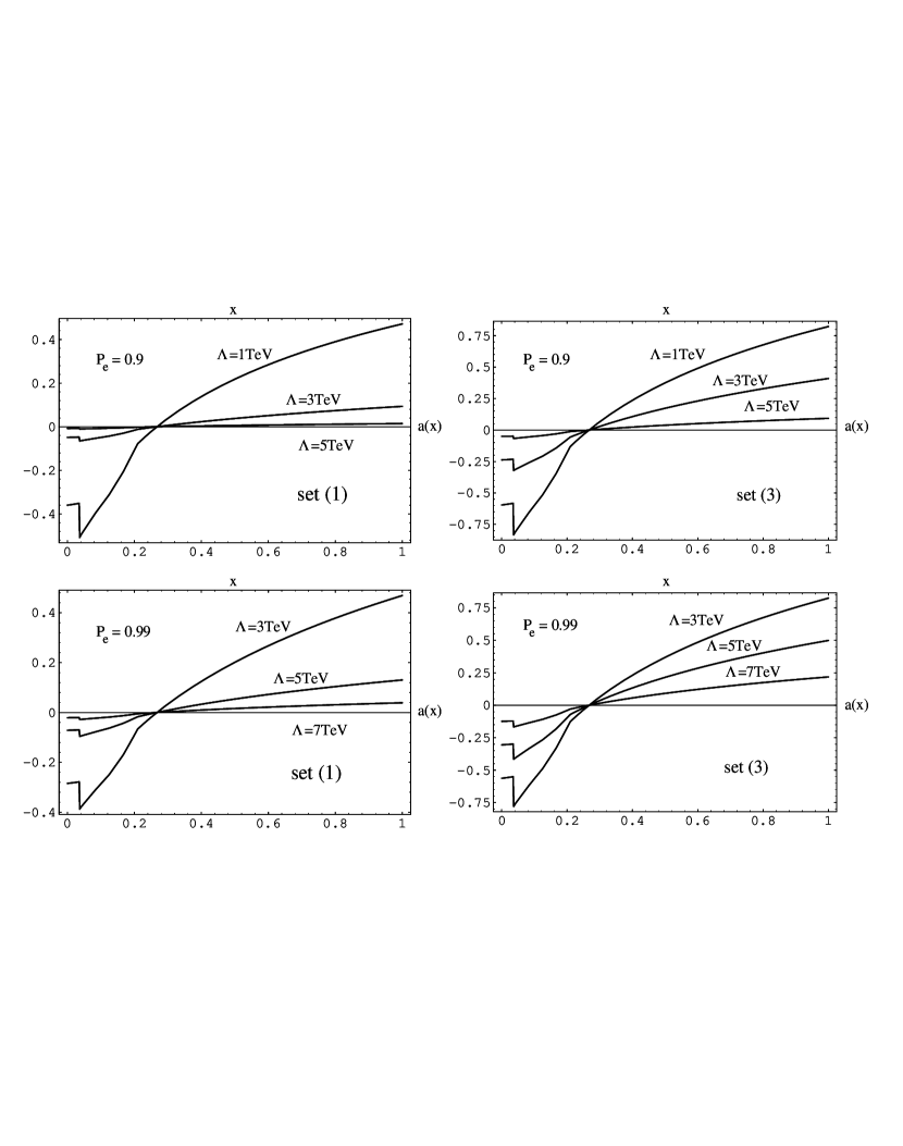
Figure 1: The asymmetry $a(x)$ for initial polarization $P_{e}(=P_{e^{-}}=-P_{e^{+}})=0.9\;\hbox{and}\;0.99$, $\sqrt{s}=500$ GeV, ${\mit\Lambda}=1\sim 7$ TeV and for the coefficient sets (1) and (3). The step-function-like change in the curves at $x=0.035$ is due to the SM-threshold.

Indeed the asymmetry seems to be a good measure of $\xi^{(*)}$ which receives contributions only from the scalar-tensor operators. It should be noticed, however, that the value of $\xi^{(*)}$ depends very strongly on initial-lepton-beam polarizations, effectively it is non-vanishing only in the vicinity of $P_{e^{\pm}}=1$; at least one beam must be polarized. Figure 1 shows $a(x)\,$ for various values of ${\mit\Lambda}$, $P_{e}(=P_{e^{-}}=-P_{e^{+}})=0.9$ and 0.99, and two coefficient sets (1) and (3). Here the coefficient set (3) has been adopted to avoid an accidental cancellation between $\alpha_{lq}$ and $\alpha_{lq^{\prime}}$ in the value of $S_{LL}$ (see eq.(4)). In fact it is seen from the figure that the asymmetry for the set (3) gains an extra factor of about 2 in comparison with the set (1). An increase of $P_{e}$ enhances the relative strength of the new-physics effects (from scalar- and tensor-operators), because the opposite polarization of initial $e^{\pm}$ beams reduces the SM (or more generally vector-operator) contribution. Thus it causes an intensification of $a(x)$ dependence on the new-physics energy scale ${\mit\Lambda}$, as seen from the figure. Therefore large $P_{e}$ allows to penetrate higher energy scales.

Figure 2: The asymmetry $a(x)$ for unpolarized positron and polarized electron beam ($P_{e^{-}}=0.5\;\hbox{and}\;0.9$), $\sqrt{s}=500$ GeV, ${\mit\Lambda}=1\sim 3$ TeV and for the coefficient sets (1) and (3).

One should, however, keep also in mind that increasing opposite polarization of both beams we suppress the (SM-like) vector-operator contributions and therefore the total number of events is strongly reduced, see Tab.4, so the measurement of the asymmetry will be a challenging task for experimentalists. Therefore it is instructive to consider unpolarized positron beam. Besides, in practice it appears to be much more difficult to achieve positron polarization, so below we also present results for unpolarized positron beams.

$P_{e}$	${\mit\Lambda}$ (TeV)
	3	5	7	SM
0	0.68	0.61	0.59	0.58
0.5	0.51	0.46	0.45	0.44
0.9	0.14	0.12	0.11	0.11
0.99	0.03	0.01	0.01	0.01

Table 4: The total cross section $\sigma(e^{+}e^{-}\to t\bar{t})$ in pb with $\sqrt{s}=500$ GeV, for ${\mit\Lambda}=3,\>5,\>7$ TeV with the coefficient set (1) and the SM, for polarization $P_{e}(=P_{e^{-}}=-P_{e^{+}})=0.0,\;0.5,\;0.9,\;0.99$. Here we used $\alpha(s)(\simeq 1/126)$ instead of $\alpha(0)$.

It is seen from the plots in Figs.1, 2 that the typical size of the asymmetry for unpolarized positrons is smaller than the one for opposite electron and positron polarization, therefore sensitivity of the asymmetry to non-standard physics embedded in the coefficients $S$ and $T$ is being reduced. The reason is that for $P_{e}^{+}=0$ the parameter $\xi^{(*)}$ defined by eq.(10) is suppressed by non-zero SM contributions. However, one can observe that for the set (3), $P_{e^{-}}=0.9$, $\sqrt{s}=500$ GeV and ${\mit\Lambda}=1$ TeV the asymmetry could be still large, of the order of $50\%$. One can conclude that in order to penetrate physics up to ${\mit\Lambda}=2$  TeV at $\sqrt{s}=500$ GeV electron polarization greater than $P_{e^{-}}=0.9$ would be needed.

5. Summary

Next-generation linear colliders of $e^{+}e^{-}$, NLC, will provide the cleanest environment for studying top-quark interactions. There, we shall be able to perform detailed tests of top-quark couplings and either confirm the SM simple generation-repetition pattern or discover some non-standard interactions. In this paper, we focused on the four-Fermi-type new interactions, and studied their possible effects in $e^{+}e^{-}\to t\bar{t}\to\ell^{\pm}\cdots$ for arbitrary longitudinal beam polarizations. Then, the recently proposed optimal-observables technique [5] has been adopted to determine non-standard couplings through single-leptonic-spectrum measurements.

There are scalar-, vector- and tensor-type four-Fermi interactions contributing to our process. Since the first and last ones do not interfere with the standard contribution, their effects were found too small to be detected directly in the secondary-lepton-energy spectrum, though the details depend on the size of the new-physics scale ${\mit\Lambda}$. On the other hand, the vector interactions can interfere with the SM contributions, so there seems to be a chance to detect their effects through the optimal observables if ${\mit\Lambda}$ is not too high; e.g. ${\mit\Lambda}\lower 2.15277pt\hbox{$\>\buildrel<\over{\sim}\>$}3$ TeV may provide $4\sigma$ effects at $\sqrt{s}=500$ GeV.

In order to detect a signal of the scalar- and tensor-interactions, we considered the lepton-energy asymmetry $a(x)$. We conclude that the asymmetry might be useful when we achieve highly polarized $e^{\pm}$ beams. Indeed, we found that at $\sqrt{s}=500$ GeV $a(x)$ becomes of the order of $25\,\%$ even for ${\mit\Lambda}=3$ TeV when both beams are polarized simultaneously to $P_{e}(=P_{e^{+}}=P_{e^{-}})=0.9$. High polarization of positron beam is hard to realize, however we found that the use of polarized $e^{-}$ beam is still effective even when $P_{e^{+}}=0$. For example, the size of $a(x)$ could reach $50\%$ for ${\mit\Lambda}=1$ TeV for $P_{e^{-}}=0.9$.

ACKNOWLEDGMENTS

This work is supported in part by the State Committee for Scientific Research (Poland) under grant 2 P03B 180 09 and by Maria Skłodowska-Curie Joint Fund II (Poland-USA) under grant MEN/NSF-96-252.

Appendix A. Differential cross section for $\mbox{\boldmath$e$}^{+}\mbox{\boldmath$e$}^{-}\to\mbox{\boldmath$t$}\bar{\mbox{\boldmath$t$}}$

The differential cross section for $e^{+}e^{-}\to t\bar{t}$ as a function of $P\equiv p_{e^{-}}+p_{e^{+}}$, $l\equiv p_{e^{-}}-p_{e^{+}}$, $q\equiv p_{t}-p_{\bar{t}}$, the longitudinal polarization ${P_{e^{-}}}({P_{e^{+}}})$ of the initial electron (positron) beam and spin 4-vectors $s_{+}(s_{-})$ of $t(\bar{t})$ taking into account corrections from four-Fermi operators (3) is given by the following formula:
(1) Scalar-Tensor operators :

$$\frac{d\sigma}{d\Omega_{t}}^{\!\!ST}\!\!\!\!({P_{e^{-}}},{P_{e^{+}}},s_{+},s_{-})$$

$$=\frac{3\beta}{512\pi^{2}s}\Bigl{[}\>\>(1-{P_{e^{-}}}{P_{e^{+}}})[\>|S\,|^{2}s\{s-2m_{t}^{2}(1-s_{+}s_{-})\}$$

$$\ \ \ \ \ \ \ \;\;\;\;\;\;\;\;\;\;+4\,|\,T\,|^{2}\{2m_{t}^{2}s(1-s_{+}s_{-})+(lq)^{2}+4m_{t}^{2}(Ps_{+}\;Ps_{-}-ls_{+}\;ls_{-})\}$$

$$\ \ \ \ \ \ \ \;\;\;\;\;\;\;\;\;\;+4\,{\rm Re}(ST^{*})\{lq\>s+2m_{t}^{2}(ls_{+}\;Ps_{-}-Ps_{+}\;ls_{-})\}$$

$$\ \ \ \ \ \ \ \;\;\;\;\;\;\;\;\;\;+8\,{\rm Im}(ST^{*})m_{t}^{2}\epsilon(s_{+},s_{-},P,l)\>]$$

$$\ \ \ \ \ \ \ -2({P_{e^{-}}}-{P_{e^{+}}})m_{t}[\>|S\,|^{2}s(Ps_{+}+Ps_{-})+4\,|\,T\,|^{2}lq(ls_{+}-ls_{-})$$

$$\ \ \ \ \ \ \ \;\;\;\;\;\;\;\;\;\;+2\,{\rm Re}(ST^{*})\{s(ls_{+}-ls_{-})+lq(Ps_{+}+Ps_{-})\}$$

$$\ \ \ \ \ \ \ \;\;\;\;\;\;\;\;\;\;+2\,{\rm Im}(ST^{*})\{\epsilon(s_{+},P,q,l)+\epsilon(s_{-},P,q,l)\}\>]\>\>\Bigr{]}.$$ (14)

(2) Standard Model plus Vector operators :

$$\frac{d\sigma}{d\Omega_{t}}^{\!\!S\!M+V}\!\!\!\!\!\!\!\!\!\!({P_{e^{-}}},{P_{e^{+}}},s_{+},s_{-})$$

$$=\frac{3\beta\alpha^{2}}{16s^{3}}\>\Bigl{[}\>\>D_{V}^{(*)}\>[\>\{4m_{t}^{2}s+(lq)^{2}\}(1-s_{+}s_{-})+s^{2}(1+s_{+}s_{-})$$

$$\ \ \ \;\;\;\;\;\;\;\;\;\;+2s(ls_{+}\;ls_{-}-Ps_{+}\;Ps_{-})+\>2\,lq(ls_{+}\;Ps_{-}-ls_{-}\;Ps_{+})\>]$$

$$\ \ \ +\>D_{A}^{(*)}\>[\>(lq)^{2}(1+s_{+}s_{-})-(4m_{t}^{2}s-s^{2})(1-s_{+}s_{-})$$

$$\ \ \ \;\;\;\;\;\;\;\;\;\;-2(s-4m_{t}^{2})(ls_{+}\;ls_{-}-Ps_{+}\;Ps_{-})-\>2\,lq(ls_{+}\;Ps_{-}-ls_{-}\;Ps_{+})\>]$$

$$\ \ \ -4\>{\rm Re}(D_{V\!\!A}^{(*)})\>m_{t}\,[\>s(Ps_{+}-Ps_{-})+lq(ls_{+}+ls_{-})\>]$$

$$\ \ \ +2\>{\rm Im}(D_{V\!\!A}^{(*)})\>[\>lq\,\epsilon(s_{+},s_{-},q,l)+ls_{-}\epsilon(s_{+},P,q,l)+ls_{+}\epsilon(s_{-},P,q,l)\>]$$

$$\ \ \ +4\>E_{V}^{(*)}\>m_{t}s(ls_{+}+ls_{-})+4\>E_{A}^{(*)}\>m_{t}\,lq(Ps_{+}-Ps_{-})$$

$$\ \ \ +4\>{\rm Re}(E_{V\!\!A}^{(*)})\>[\>2m_{t}^{2}(ls_{+}\;Ps_{-}-ls_{-}\;Ps_{+})-lq\>s\>]$$

$$\ \ \ +4\>{\rm Im}(E_{V\!\!A}^{(*)})\>m_{t}[\>\epsilon(s_{+},P,q,l)+\epsilon(s_{-},P,q,l)\>]\>\>\Bigr{]},$$ (15)

where

$$\,D^{(*)}_{V}=(1+{P_{e^{-}}}{P_{e^{+}}})\Bigl{[}\>\Bigl{|}v_{e}v_{t}d-e_{t}+\frac{A_{L}+A_{R}}{4}\frac{s}{e^{2}}\Bigr{|}^{2}+\Bigl{|}a_{e}v_{t}d+\frac{A_{L}-A_{R}}{4}\frac{s}{e^{2}}\Bigr{|}^{2}\>\Bigr{]}$$

$$\;\;\;\;\;\;\;\;\;\;-2\,({P_{e^{-}}}+{P_{e^{+}}})\>{\rm Re}\Bigl{[}(v_{e}v_{t}d-e_{t}+\frac{A_{L}+A_{R}}{4}\frac{s}{e^{2}})(a_{e}v_{t}d+\frac{A_{L}-A_{R}}{4}\frac{s}{e^{2}})^{*}\Bigr{]},$$

$$\,D^{(*)}_{A}=(1+{P_{e^{-}}}{P_{e^{+}}})\Bigl{[}\>\Bigl{|}v_{e}a_{t}d+\frac{B_{L}+B_{R}}{4}\frac{s}{e^{2}}\Bigr{|}^{2}+\Bigl{|}a_{e}a_{t}d+\frac{B_{L}-B_{R}}{4}\frac{s}{e^{2}}\Bigr{|}^{2}\>\Bigr{]}$$

$$\;\;\;\;\;\;\;\;\;\;-2\,({P_{e^{-}}}+{P_{e^{+}}})\>{\rm Re}\Bigl{[}(v_{e}a_{t}d+\frac{B_{L}+B_{R}}{4}\frac{s}{e^{2}})(a_{e}a_{t}d+\frac{B_{L}-B_{R}}{4}\frac{s}{e^{2}})^{*}\Bigr{]},$$

$$\,D^{(*)}_{V\!A}=(1+{P_{e^{-}}}{P_{e^{+}}})\Bigl{[}\>(v_{e}a_{t}d+\frac{B_{L}+B_{R}}{4}\frac{s}{e^{2}})(v_{e}v_{t}d-e_{t}+\frac{A_{L}+A_{R}}{4}\frac{s}{e^{2}})^{*}$$

$$\;\;\;\;\;\;\;\;\;\;\;\;\;\;\;\;\;\;\;\;+(a_{e}a_{t}d+\frac{B_{L}-B_{R}}{4}\frac{s}{e^{2}})(a_{e}v_{t}d+\frac{A_{L}-A_{R}}{4}\frac{s}{e^{2}})^{*}\>\Bigr{]}$$

$$\;\;\;\;\;\;\;\;\;\;-({P_{e^{-}}}+{P_{e^{+}}})\Bigl{[}\>(v_{e}a_{t}d+\frac{B_{L}+B_{R}}{4}\frac{s}{e^{2}})(a_{e}v_{t}d+\frac{A_{L}-A_{R}}{4}\frac{s}{e^{2}})^{*}$$

$$\;\;\;\;\;\;\;\;\;\;\;\;\;\;\;\;\;\;\;\;+(a_{e}a_{t}d+\frac{B_{L}-B_{R}}{4}\frac{s}{e^{2}})(v_{e}v_{t}d-e_{t}+\frac{A_{L}+A_{R}}{4}\frac{s}{e^{2}})^{*}\>\Bigr{]},$$

$$\,E^{(*)}_{V}=2\,(1+{P_{e^{-}}}{P_{e^{+}}})\>{\rm Re}\Bigl{[}(v_{e}v_{t}d-e_{t}+\frac{A_{L}+A_{R}}{4}\frac{s}{e^{2}})(a_{e}v_{t}d+\frac{A_{L}-A_{R}}{4}\frac{s}{e^{2}})^{*}\Bigr{]}$$

$$\;\;\;\;\;\;\;\;\;\;-({P_{e^{-}}}+{P_{e^{+}}})\Bigl{[}\>\Bigl{|}v_{e}v_{t}d-e_{t}+\frac{A_{L}+A_{R}}{4}\frac{s}{e^{2}}\Bigr{|}^{2}+\Bigl{|}a_{e}v_{t}d+\frac{A_{L}-A_{R}}{4}\frac{s}{e^{2}}\Bigr{|}^{2}\>\Bigr{]},$$

$$\,E^{(*)}_{A}=2\,(1+{P_{e^{-}}}{P_{e^{+}}})\>{\rm Re}\Bigl{[}(v_{e}a_{t}d+\frac{B_{L}+B_{R}}{4}\frac{s}{e^{2}})(a_{e}a_{t}d+\frac{B_{L}-B_{R}}{4}\frac{s}{e^{2}})^{*}\Bigr{]}$$

$$\;\;\;\;\;\;\;\;\;\;-({P_{e^{-}}}+{P_{e^{+}}})\Bigl{[}\>\Bigl{|}v_{e}a_{t}d+\frac{B_{L}+B_{R}}{4}\frac{s}{e^{2}}\Bigr{|}^{2}+\Bigl{|}a_{e}a_{t}d+\frac{B_{L}-B_{R}}{4}\frac{s}{e^{2}}\Bigr{|}^{2}\>\Bigr{]},$$

$$\,E^{(*)}_{V\!A}=(1+{P_{e^{-}}}{P_{e^{+}}})\Bigl{[}\>(v_{e}a_{t}d+\frac{B_{L}+B_{R}}{4}\frac{s}{e^{2}})(a_{e}v_{t}d+\frac{A_{L}-A_{R}}{4}\frac{s}{e^{2}})^{*}$$

$$\;\;\;\;\;\;\;\;\;\;\;\;\;\;\;\;\;\;\;\;+(a_{e}a_{t}d+\frac{B_{L}-B_{R}}{4}\frac{s}{e^{2}})(v_{e}v_{t}d-e_{t}+\frac{A_{L}+A_{R}}{4}\frac{s}{e^{2}})^{*}\>\Bigr{]}$$

$$\;\;\;\;\;\;\;\;\;\;-({P_{e^{-}}}+{P_{e^{+}}})\Bigl{[}\>(v_{e}a_{t}d+\frac{B_{L}+B_{R}}{4}\frac{s}{e^{2}})(v_{e}v_{t}d-e_{t}+\frac{A_{L}+A_{R}}{4}\frac{s}{e^{2}})^{*}$$

$$\;\;\;\;\;\;\;\;\;\;\;\;\;\;\;\;\;\;\;\;+(a_{e}a_{t}d+\frac{B_{L}-B_{R}}{4}\frac{s}{e^{2}})(a_{e}v_{t}d+\frac{A_{L}-A_{R}}{4}\frac{s}{e^{2}})^{*}\>\Bigr{]},$$

with

$$d\equiv\frac{s}{s-M_{Z}^{2}}\frac{1}{16\sin^{2}\theta_{W}\cos^{2}\theta_{W}},$$

$$v_{f}\equiv 2I^{f}_{3}-4e_{f}\sin^{2}\theta_{W},\ \ a_{f}\equiv 2I^{f}_{3},$$

$I^{f}_{3}=\pm 1/2$ for up or down particles, and $e_{f}$ is an electric charge in units of the electric charge of the proton. The symbol $\epsilon(a,b,c,d)$ means $\epsilon_{\mu\nu\rho\sigma}a^{\mu}b^{\nu}c^{\rho}d^{\sigma}$ with $\epsilon_{0123}=+1$. The longitudinal polarizations of electrons and positrons are by definition:

$${P_{e^{-}}}=\frac{N_{1+}-N_{1-}}{N_{1+}+N_{1-}},\ \ \ {P_{e^{+}}}=-\frac{N_{2+}-N_{2-}}{N_{2+}+N_{2-}}$$

with

$\bullet~{}N_{1+}$ number of electrons with helicity +

$\bullet~{}N_{1-}$ number of electrons with helicity $-$

$\bullet~{}N_{2+}$ number of positrons with helicity +

$\bullet~{}N_{2-}$ number of positrons with helicity $-$

Appendix B. Differential decay rate for an unpolarized top quark

The differential decay rates for an unpolarized $t$ and $\bar{t}$ quark including the Standard Model and four-Fermi operators (6) are both given by:

$$\frac{1}{{\mit\Gamma}_{t}}\frac{d^{2}{\mit\Gamma}_{\ell}}{dxd\omega}(\stackrel{{\scriptstyle\scriptscriptstyle(-)}}{{t}}\!(p_{t})\to\ell^{\pm}(p_{\ell})X)$$

$$\ \ \ =\frac{1+\beta}{\beta}B_{\ell}\Bigl{[}\>\frac{3}{W}\alpha_{0}\omega\;\theta(1-r-\omega)\;\theta\Bigl{(}x-r\frac{1-\beta}{1+\beta}\Bigr{)}+\sum_{i=1}^{3}\alpha^{4F}_{i}\omega^{i-1}\>\Bigr{]},$$ (16)

where $\omega\equiv(p_{t}-p_{\ell})^{2}/m_{t}^{2}$, ${\mit\Gamma}_{t}$ is the total width of $t$,

$$\alpha_{0}=\frac{G}{G+2(|S^{D}\,|^{2}+|S^{D}_{RL}\,|^{2}+4|\,V^{D}\,|^{2}+12|\,T^{D}\,|^{2})},$$

$$\alpha^{4F}_{1}=2\frac{|S^{D}\,|^{2}+|S^{D}_{RL}\,|^{2}+4|\,T^{D}\,|^{2}+4\,{\rm Re}(S^{D}T^{D*})}{G+2(|S^{D}\,|^{2}+|S^{D}_{RL}\,|^{2}+4|\,V^{D}\,|^{2}+12|\,T^{D}\,|^{2})},$$

$$\alpha^{4F}_{2}=2\frac{|S^{D}\,|^{2}+|S^{D}_{RL}\,|^{2}+24|\,V^{D}\,|^{2}+52|\,T^{D}\,|^{2}-20\,{\rm Re}(S^{D}T^{D*})}{G+2(|S^{D}\,|^{2}+|S^{D}_{RL}\,|^{2}+4|\,V^{D}\,|^{2}+12|\,T^{D}\,|^{2})},$$

$$\alpha^{4F}_{3}=-4\frac{|S^{D}\,|^{2}+|S^{D}_{RL}\,|^{2}+12|\,V^{D}\,|^{2}+28|\,T^{D}\,|^{2}-8\,{\rm Re}(S^{D}T^{D*})}{G+2(|S^{D}\,|^{2}+|S^{D}_{RL}\,|^{2}+4|\,V^{D}\,|^{2}+12|\,T^{D}\,|^{2})},$$

and

$$G\equiv\frac{4\pi g^{4}W}{m_{t}^{2}M_{W}{\mit\Gamma}_{W}},\ \ \ W\equiv(1-r)^{2}(1+2r),\ \ \ r\equiv(M_{W}/m_{t})^{2}.$$

Note that $\alpha_{0}$ and $\alpha^{4F}_{i}$ satisfy

$$\alpha_{0}+\alpha^{4F}_{1}+\frac{1}{3}\alpha^{4F}_{2}+\frac{1}{6}\alpha^{4F}_{3}=1.$$ (17)

As is seen from $\alpha_{0}$ and $\alpha^{4F}_{i}$, the first term in eq.(16) (with two $\theta$-functions) is the SM contribution and the second term is from the four-Fermi operators. Since we used the narrow-width approximation in the SM part, the ranges of $x$ and $\omega$ there are different from those in the second term. The two $\theta$-functions express this difference. See appendices C and D for more details.

Appendix C. Functions $\mbox{\boldmath$f$}(\!\!(\mbox{\boldmath$x$})\!\!)$ and $\mbox{\boldmath$g$}(\!\!(\mbox{\boldmath$x$})\!\!)$

The functions $f(x)$ and $g(x)$ are defined as

$$f(x)\equiv\frac{3}{W}\frac{1+\beta}{\beta}\int d\omega\,\omega,$$ (18)

$$g(x)\equiv\frac{3}{W}\frac{1+\beta}{\beta}\int d\omega\,\omega\Bigl{[}\>1-\frac{x(1+\beta)}{1-\omega}\>\Bigr{]}.$$ (19)

The variable $\omega$ is constrained by the inequalities

$$0\leq\omega\leq 1-r\ \ \ {\rm and}\ \ \ 1-x\frac{1+\beta}{1-\beta}\leq\omega\leq 1-x$$

while the reduced energy is bounded by

$$r\frac{1-\beta}{1+\beta}\leq x\leq 1.$$

Carrying out the integration yields

$$f(x)={3\over{W}}{{1+\beta}\over{2\beta}}\,\Bigl{[}\>r(r-2)+2x{{1+\beta}\over{1-\beta}}-x^{2}\Bigl{(}{{1+\beta}\over{1-\beta}}\Bigr{)}^{2}\>\Bigr{]},$$

$$\hskip 223.06949pt({\rm for\ the\ interval}\ I_{1},\ I_{4})$$

$$\phantom{f(x)}={3\over{W}}{{1+\beta}\over{2\beta}}\,(1-r)^{2},\hskip 91.6179pt({\rm for\ the\ interval}\ I_{2})$$

$$\phantom{f(x)}={3\over{W}}{{1+\beta}\over{2\beta}}\,(1-x)^{2},\hskip 90.47955pt({\rm for\ the\ interval}\ I_{3},\ I_{6})$$

$$\phantom{f(x)}=\frac{6}{W}\frac{1+\beta}{(1-\beta)^{2}}\,x(1-\beta-x),\hskip 52.63777pt({\rm for\ the\ interval}\ I_{5})$$

$$g(x)={3\over{W}}{{(1+\beta)^{2}}\over\beta}\,\Bigl{[}\>-rx+x^{2}{{1+\beta}\over{1-\beta}}-x\ln{{x(1+\beta)}\over{r(1-\beta)}}$$

$$\phantom{g(x)}\ \ \ \ \ \ \ \ +{1\over{2(1+\beta)}}\Bigl{\{}\>r(r-2)+2x{{1+\beta}\over{1-\beta}}-x^{2}\Bigl{(}{{1+\beta}\over{1-\beta}}\Bigr{)}^{2}\>\Bigr{\}}\>\Bigr{]},$$

$$\hskip 241.84842pt({\rm for\ the\ interval}\ I_{1},\ I_{4})$$

$$\phantom{g(x)}={3\over{W}}{{(1+\beta)^{2}}\over\beta}\,\Bigl{[}\>(1-r+\ln r)x+{1\over{2(1+\beta)}}(1-r)^{2}\>\Bigr{]},$$

$$\hskip 241.84842pt({\rm for\ the\ interval}\ I_{2})$$

$$\phantom{g(x)}={3\over{W}}{{(1+\beta)^{2}}\over\beta}\,\Bigl{[}\>(1-x+\ln x)x+{1\over{2(1+\beta)}}(1-x)^{2}\>\Bigr{]},$$

$$\hskip 241.84842pt({\rm for\ the\ interval}\ I_{3},\ I_{6})$$

$$\phantom{g(x)}=\frac{3}{W}\frac{1+\beta}{\beta(1-\beta)^{2}}\,x\Bigl{[}\>2\beta(1-\beta-\beta^{2}x)-(1+\beta)(1-\beta)^{2}\ln{{1+\beta}\over{1-\beta}}\>\Bigr{]},$$

$$\hskip 241.84842pt({\rm for\ the\ interval}\ I_{5})$$

where $I_{i}(i=1\sim 6)$ are given by

$$I_{1}:r(1-\beta)/(1+\beta)\leq x\leq(1-\beta)/(1+\beta),$$

$$I_{2}:(1-\beta)/(1+\beta)\leq x\leq r,$$

$$I_{3}:r\leq x\leq 1,$$

($I_{1,2,3}$ are for $r\geq(1-\beta)/(1+\beta)$)

$$I_{4}:r(1-\beta)/(1+\beta)\leq x\leq r,$$

$$I_{5}:r\leq x\leq(1-\beta)/(1+\beta),$$

$$I_{6}:(1-\beta)/(1+\beta)\leq x\leq 1,$$

($I_{4,5,6}$ are for $r\leq(1-\beta)/(1+\beta)$).
Note that $f(x)$ and $g(x)$ satisfy

$$\int f(x)dx=1,\ \ \ \ \int g(x)dx=0.$$ (20)

Appendix D. Functions $\mbox{\boldmath$f$}^{{\bf 4}F\!\!\!\!\!F}(\!\!(\mbox{\boldmath$x$})\!\!)$ and $\mbox{\boldmath$g$}^{{\bf 4}F\!\!\!\!\!\!\,F}(\!\!(\mbox{\boldmath$x$})\!\!)$

The functions $f^{4F}_{i}(x)$ and $g^{4F}_{i}(x)$ (for $i=1\sim 3$) are defined as

$$f^{4F}_{i}(x)\equiv\frac{1+\beta}{\beta}\int d\omega\,\omega^{i-1},$$ (21)

$$g^{4F}_{i}(x)\equiv\frac{1+\beta}{\beta}\int d\omega\,\omega^{i-1}\Bigl{[}\>1-\frac{x(1+\beta)}{1-\omega}\>\Bigr{]}.$$ (22)

The variable $\omega$ is constrained by the inequalities

$$0\leq\omega\leq 1\ \ \ {\rm and}\ \ \ 1-x\frac{1+\beta}{1-\beta}\leq\omega\leq 1-x$$

while the reduced energy is bounded by

$$0\leq x\leq 1.$$

Carrying out the integration yields

$$f^{4F}_{1}(x)=\frac{2(1+\beta)}{1-\beta}\,x,$$

$$f^{4F}_{2}(x)=\frac{2(1+\beta)}{(1-\beta)^{2}}\,x(1-\beta-x),$$

$$f^{4F}_{3}(x)=\frac{2(1+\beta)}{3(1-\beta)^{3}}\,x\bigl{[}\>3(1-\beta)(1-\beta-2x)$$

$$\;\;\;\;\;\;\;\;\;\;\;\;\;\;\;\;\;\;\;\;+(3+\beta^{2})x^{2}\>\bigr{]}, I^{4F}_{1}$$ ( for the interval  )

$$f^{4F}_{1}(x)=\frac{1+\beta}{\beta}(1-x),$$

$$f^{4F}_{2}(x)=\frac{1+\beta}{2\beta}(1-x)^{2},$$

$$f^{4F}_{3}(x)=\frac{1+\beta}{3\beta}(1-x)^{3},~{}~{}~{}~{}~{}~{}~{}~{}~{}~{}~{} I^{4F}_{2}$$ ( for the interval  )

Figure 3: The functions $f^{4F}_{i}(x)$.

$$g^{4F}_{1}(x)=\frac{1+\beta}{\beta(1-\beta)}\,x\Bigl{[}\>2\beta+(1-\beta^{2})\ln\frac{1-\beta}{1+\beta}\>\Bigr{]},$$

$$g^{4F}_{2}(x)=\frac{1+\beta}{\beta(1-\beta)^{2}}\,x\Bigl{[}\>2\beta(1-\beta-\beta^{2}x)+(1+\beta)(1-\beta)^{2}\ln\frac{1-\beta}{1+\beta}\>\Bigr{]},$$

$$g^{4F}_{3}(x)=\frac{1+\beta}{3\beta(1-\beta)^{3}}\,x\Bigl{[}\>6\beta(1-\beta)(1-\beta-2\beta^{2}x)+8\beta^{3}x^{2}$$

$$\;\;\;\;\;\;\;\;\;\;\;\;\;\;\;\;\;\;\;\;+3(1+\beta)(1-\beta)^{3}\ln\frac{1-\beta}{1+\beta}\>\Bigr{]}, I^{4F}_{1}$$ ( for the interval  )

$$g^{4F}_{1}(x)=\frac{1+\beta}{\beta}\bigl{[}\,1-x+(1+\beta)x\ln\,x\,\bigr{]},$$

$$g^{4F}_{2}(x)=\frac{1+\beta}{2\beta}\bigl{[}\,1+2\beta x-(1+2\beta)x^{2}+2(1+\beta)x\ln\,x\,\bigr{]},$$

$$g^{4F}_{3}(x)=\frac{1+\beta}{6\beta}\bigl{[}\,2+3(1+3\beta)x-6(1+2\beta)x^{2}+(1+3\beta)x^{3}$$

$$\;\;\;\;\;\;\;\;\;\;\;\;\;\;\;\;\;\;\;\;+6(1+\beta)x\ln\,x\,\bigr{]},~{}~{} I^{4F}_{2}$$ ( for the interval  )

where $I_{i}^{4F}\>(i=1,\>2)$ are given by

$$I_{1}^{4F}:\ 0\leq x\leq\frac{1-\beta}{1+\beta},\ \ \ I_{2}^{4F}:\ \frac{1-\beta}{1+\beta}\leq x\leq 1.$$

Note that $f^{4F}_{i}(x)$ and $g^{4F}_{i}(x)$ satisfy

$$\begin{array}[]{ll}\displaystyle\int f^{4F}_{1}(x)dx=1,{}{}{}&\displaystyle\int f^{4F}_{2}(x)dx=\displaystyle\frac{1}{3},\\ \displaystyle\int f^{4F}_{3}(x)dx=\displaystyle\frac{1}{6},&\displaystyle\int g^{4F}_{i}(x)dx=0,\end{array}$$ (23)

for $i=1\sim 3$.

Figure 4: The functions $g^{4F}_{i}(x)$.

References

• [1] W. Buchmüller and D. Wyler, Nucl. Phys. B268 (1986), 621.
See also
C.J.C. Burges and H.J. Schnitzer, Nucl. Phys. B228 (1983), 464;
C.N. Leung, S.T. Love and S. Rao, Z. Phys. C31 (1986), 433.
• [2] B. Grza̧dkowski and Z. Hioki, Nucl. Phys. B484 (1997), 17 (hep-ph/9604301).
• [3] B. Grza̧dkowski and Z. Hioki, Phys. Lett. B391 (1997), 172 (hep-ph/9608306).
• [4] L. Brzeziński, B. Grza̧dkowski and Z. Hioki, Preprint IFT-10-97 – TOKUSHIMA 97-01 (hep-ph/9710358).
• [5] J.F. Gunion, B. Grza̧dkowski and X-G. He, Phys. Rev. Lett. 77 (1996), 5172 (hep/ph-9605326).
• [6] B. Grza̧dkowski, Acta Phys. Pol. B27 (1996), 921 (hep-ph/9511279).
• [7] C. Arzt, M.B. Einhorn and J. Wudka, Nucl. Phys. B433 (1995), 41 (hep-ph/9405214).
• [8] S. Kawasaki, T. Shirafuji and S.Y. Tsai, Prog. Theor. Phys. 49 (1973), 1656.
• [9] Particle Data Group : R.M. Barnett et al., Review of Particle Properties, Phys. Rev. D54 (1996), PART I.
• [10] T. Arens and L.M. Sehgal, Phys. Rev. D50 (1994), 4372.
• [11] All electroweak data (except for ${\mit\Gamma}_{W}$ [9]) are taken from:
Talks by G. Altarelli, by P. Giromini, by Y.Y. Kim, and by J. Timmermans at XVIII International Symposium on Lepton-Photon Interactions, Jul.28 - Aug.1, 1997, Hamburg, Germany.
• [12] D. Chang, W.-Y. Keung and I. Phillips, Nucl. Phys. B408 (1993), 286 (hep-ph/9301259); ibid. B429(1994), 255(Erratum).