FERMILAB-Pub-97/413-T

DTP/97/114

Probabilistic Jet Algorithms
W. T. Giele¹ and E. W. N.  Glover^2
1Fermi National Accelerator Laboratory, P. O. Box 500, Batavia, IL 60510, U.S.A.

²Physics Department, University of Durham, Durham DH1 3LE, England

Conventional jet algorithms are based on a deterministic view of the underlying hard scattering process. Each outgoing parton from the hard scattering is associated with a hard, well separated jet. This approach is very successful because it allows quantitative predictions using lowest order perturbation theory. However, beyond leading order in the coupling constant, when quantum fluctuations are included, deterministic jet algorithms will become problematic precisely because they attempt to describe an inherently stochastic quantum process using deterministic, classical language. This demands a shift in the way we view jet algorithms. We make a first attempt at constructing more probabilistic jet algorithms that reflect the properties of the underlying hard scattering and explore the basic properties and problems of such an approach.

In high momentum transfer scattering processes, the concept of jets makes a connection between the hadron-level observations and the underlying partonic theory. For “good” observables the theory is perturbatively calculable and, at lowest order (LO) in the coupling constant, the predictions are deterministic due to the absence of quantum fluctuations. Each parton is associated with a high momentum jet. After “hadronizing” the parton, one ends up with a collimated shower of hadrons. Often color strings of hadrons between the partons are introduced to model the energy flows better. However, the underlying hard scattering in such an approach is still classical. Conventional jet algorithms are based on these models. Their main purpose is to “invert” the hadronization and identify the underlying hard scattering parton structure. Within the classical approach this is perfectly legitimate. In fact, jet algorithms are often compared by how well they reconstruct the underlying partonic structure. Moreover, experimenters use shower models such as HERWIG [1] to estimate their theory/experimental uncertainties by hadronizing a parton in the detector simulation. Here the jet algorithm is applied to estimate the mismeasurement of the original parton energy and direction. One then uses such models to either “correct back” to the parton level or to absorb these effects into the systematic uncertainties.

This philosophy is acceptable as long as quantum fluctuations can be neglected. The degree to which this approximation can be applied depends on both the experimental accuracy and on the kinematics of the event (i.e. well separated hard jets are, for all practical purposes, classical.). However, when one counts jets using the classical jet algorithms, the majority of the cross section in multi-jet events comes from the region where the jet clusters are as close to each other as allowed by the jet algorithm due to the collinear behaviour of QCD. This means that quantum corrections are important as soon as the experimental uncertainties become small enough. In recent years it has become apparent that one needs at least next-to-leading order (NLO) perturbative calculations to describe the precise jet data accumulated in current high energy scattering experiments, i.e. one is sensitive to the quantum corrections. Applying the usual deterministic jet algorithms then leads to immediate problems which are exactly associated with the stochastic nature of the underlying scattering (i.e. each parton involved in the the hard scattering is no longer identifiable as a jet.). Using shower models to correct back to the “original” parton energies might be misleading. Furthermore, adding some arbitrary soft radiation or collinear fragmentation can significantly alter the jet energies and directions found using deterministic jet algorithms rendering the theoretical predictions infrared unstable. Similarly, in the experiment a single hit in the calorimeter should only be associated with a jet/cluster in a probabilistic manner since small mismeasurements will change the assignment of calorimeter hits to jets. These instabilities are reflected in large hadronization corrections and large experimental uncertainties.

The obvious way out is to introduce probabilistic jet algorithms to reflect the quantum mechanical nature of the hard scattering. On an event by event basis the algorithm will give a probability distribution to observables in the event (e.g. transverse energy, number of jets, jet-jet mass, etc.). This is contrary to classical jet algorithms which give a definite value to the observables. There will be an immediate impact on the hadronization effects and measurement errors. For example, the number of jets found using deterministic jet algorithms will always be an integer number. This number can vary on an event by event basis due to fluctuations in the hadronization process and the measurement errors (even if the underlying hard scattering is kept fixed). However with a probabilistic jet algorithm, each jet topology is associated with a probability (or equivalently the event contains a fractional number of jets). Hadronization and measurement uncertainties will still alter the probability of finding a given jet multiplicity, but now will be far less important, reflecting far more accurately the properties of the underlying quantum process. This will have some influence on observables that depend on the number of jets in the event such as the identification of top quark events. Any quantum algorithm must revert back to the classical algorithm in the limit of well separated, high energy jets (i.e. one of the jet multiplicities has a probability approaching 100%.).

Recently, Tkachov [2] has used event shape variables that satisfy calorimetric continuity (jet discriminators) to describe the jet topology of the event. Any event shape observable such as the C-parameter [3], that vanishes in the two-jet limit may be considered a three-jet discriminator. These multi particle correlators are continuous and are also stable against small variations of the input.

In the rest of the paper we will define and explore the above concepts in some detail. Also we will give an explicit example of an observable calculated with a probabilistic algorithm. This example is taken from hadron colliders: the triple differential di-jet cross section.

In order to test our ideas and to examine how hadronisation corrections influence the counting of the number of jets, we consider a simple one-dimensional toy model with two partons of energies $E_{1}$ and $E_{2}$, separated in azimuthal angle, $\phi$, by $\Delta R$, recoiling against a colour neutral object at $\phi=\pi$. Typically, we choose $E_{1}=100$ GeV and $E_{2}=50$ GeV. Although the formation of jets should not depend on the details of hadronisation, it is important to have a semi-realistic model of how the partonic energy flow fragments into hadrons. The simplest model of hadronisation is Feynman’s “tube” model [4] where a parton produces a jet of light hadrons uniformly distributed in rapidity along the jet direction. Light hadrons are distributed in transverse momentum $p_{T}$ (again with respect to the jet axis) with a gaussian density $\rho(p_{T})$ such that the average transverse momentum is controlled by the parameter, $\lambda$, that sets the hadronisation scale, $\langle p_{T}\rangle=\lambda$. Reasonable choices of $\lambda$ lie in the range $\lambda\sim 0.5-1$ GeV. We use a Monte Carlo approach to fragment the parton into several hadrons which obey the transverse momentum constraint, $\sum_{i}\vec{p}_{Ti}=\vec{0}$, where the sum runs over the hadrons produced by the parton. Each individual parton “shower” produces ${\cal O}(10)$ hadrons. This is repeated many times for each parton configuration to generate a sample of “data”.

We examine two distinct jet algorithms that are representative of those commonly used in high energy hadron collider experiments. In each case we use a cone size $R=0.7$.
(a) The fixed cone [5]. Place the cone around the highest energy particle not already in a jet and add up the energy

inside the cone. If $E>E_{\rm cut}$, it is a jet. Repeat.
(b) The iterative cone [6, 7]. Place the cone around the highest energy particle not already in a jet. Find the energy weighted axis and move the cone to that location. Repeat until jet stabilises. Repeat until no more jets are found, then resolve overlaps - i.e. for particles that are in more than one jet distribute energy amongst jets or merge clusters. Add up the energy inside the cluster and count jets with $E>E_{\rm cut}$.

At tree level, both algorithms give the same prediction for the number of jets. If the spacing between partons is less than the cone size, $\Delta R<R$, then the partons coalesce and only one jet is found. For all other values of $\Delta R$ two jets are observed. Once hadronisation is switched on (i.e. $\lambda=1$ GeV), the number of jets observed depends on exactly how the hadrons are distributed in azimuth. Generally, for $\Delta R\sim 0$ and $\Delta R\sim 2R$, either one or two jets with $E>30$ GeV are found. This is not always the case and sometimes the hadronisation pattern will cause additional jets to be found. However, for fixed intermediate values of $\Delta R$, and particularly those values close to $R$, consecutive events will flip between finding one or two jets. Depending on the actual distribution of hadrons, the topology of the event undergoes a catastrophic change. This is reflected in a large variance on the average number of jets found in the event after averaging over 10000 events. Figs. 1(a) and 2(a) illustrate this for each algorithm. By the nature of the algorithm, an integer number of jets is found in each event, but the average number (for $\Delta R\sim R$) is close to 1.5 (with a standard deviation of close to 0.5).

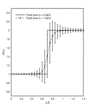
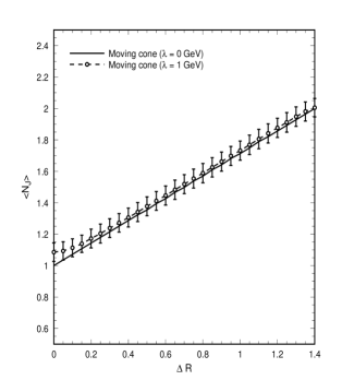
Figure 1: The average number of jets observed as a function of the parton-parton separation $\Delta R$ using the (a) fixed cone (b) moving fixed cone. The parton level results ($\lambda=0$) are shown as solid lines, while the hadron level ($\lambda=1$) predictions are shown as a dashed line joining data points with standard deviation obtained from a large number of hadronised events.

Varying the hadronisation scale $\lambda$ alters the details, but does not alter the gross feature: The individual event is not representative of the average. The problem can be traced back to the way in which the jet algorithm is applied. In each case, the starting point is the most energetic particle (or the least energetic in the case of the $K_{T}$ algorithm [8]). This choice is very sensitive to collinear fragmentation, soft radiation, the details of the hadronisation and also possible mismeasurement of the particle energy by the detector.

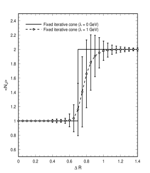
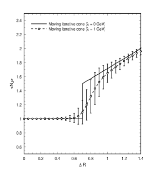
Figure 2: The average number of jets observed as a function of the parton-parton separation $\Delta R$ using the (a) iterative cone (b) moving iterative cone. The parton level results ($\lambda=0$) are shown as solid lines, while the hadron level ($\lambda=1$) predictions are shown as a dashed line joining data points with standard deviation obtained from a large number of hadronised events.

Any algorithm that requires an integer number of jets to be found in the event will have the same problems. As discussed earlier, an approach in which a probability is associated with each jet topology is more natural. We can easily adapt the existing algorithms to the probabilistic approach by treating each hadron or calorimeter cell as the seed tower for the algorithm. Each starting point will generate a particular jet configuration, and by averaging over configurations we can obtain probabilities of finding that particular jet. Because we now consider a varying starting point for each jet, we denote such algorithms as moving. The analogues of the two earlier jet algorithms are:
(A) The moving fixed cone. Center the cone on a calorimeter cell and add up the energy inside the cone. If $E>E_{\rm cut}$, it is a jet. Repeat. Repeat for all calorimeter cells.
(B) The moving iterative cone. Center the cone on a calorimeter cell. Find the energy weighted axis and move the cone to that location. Repeat until jet stabilises. If $E>E_{\rm cut}$ and the starting calorimeter cell lies within the cone, it is a jet. Repeat for all calorimeter cells. Note that even in the case of multiple clusters, there is never the issue of overlapping cones. Each calorimeter cell contributes fully to each cone containing it.
Similar probabilistic algorithms could be constructed for the $K_{T}$ or Durham algorithm [8, 9].

In each case, each starting point (and each resulting jet energy) obtains a weight of $1/2R$ to normalise the probability of finding a jet. To compute the number of jets, we count the number of calorimeter cells that give rise to an allowable jet and divide by the number of cells in $2R$ of azimuth. Even at the parton level, the algorithms behave slightly differently. For $\Delta R<R$, each calorimeter cell within $R$ of the final jet axis reconstructs the energy and direction of the parton for algorithm (B) and a single jet is found with energy $E_{1}+E_{2}$. However, for the moving cone (algorithm (A)), sometimes the cone contains one parton and sometimes two. That is to say, sometimes we find two jets, with energies $E_{1}$ and $E_{2}$ and sometimes a single jet with energy $E_{1}+E_{2}$. For $2R>\Delta R>R$, both algorithms find a combination of one-jet and two-jet configurations - calorimeter cells between the partons are more likely to result in one-jet configurations while those outside the partons will find single parton jets. For well separated partons, $\Delta R>2R$, then we always find two jets with energies $E_{1}$ and $E_{2}$. This is as it ought to be, for events with two well separated clusters should be classified as two jet events with a very high probability. Only in the intermediate regions should the one or two jet topologies have probabilities far from either 0% or 100%. At $\Delta R=R$, we see that each algorithm gives the average number of jets as 1.5. Note that this is obtained with a single event and the individual event is now representative of the average. While hadronisation will influence the formation of jets and will alter the one and two-jet probabilities, there will no longer be the catastrophic swapping between topologies. This can be seen in Figs. 1(b) and 2(b) where the average number of jets produced in the same data sample of hadronised events used earlier is plotted against the parton-parton separation, $\Delta R$. In all cases, the fluctuations are significantly smaller compared to those obtained with the corresponding conventional deterministic algorithm. Varying the hadronisation scale $\lambda$ and the jet energy cut $E_{\rm cut}$ changes the details of the plots, but in all cases, the probabilistic algorithms give smaller variances on $\langle N_{J}\rangle$ than the deterministic ones. We also see that the moving fixed cone algorithm (A) is rather good for counting clusters with an energy bigger than some threshold, but that the moving iterative cone algorithm (B) has a good jet energy resolution.

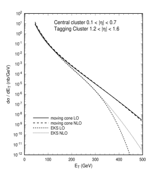
Figure 3: The leading (LO) and next-to-leading order (NLO) predictions using both the moving fixed cone and the EKS jet algorithm [13] for $\int d\eta_{1}d\eta_{2}d\sigma/dE_{T}d\eta_{1}d\eta_{2}$ for $0.1<|\eta_{1}|<0.7$ and $1.2<|\eta_{2}|<1.6$. We use CTEQ4M parton distributions [15] with renormalisation/factorisation scale $\mu=\sum E_{T}/2$.

As an example of how probabilistic algorithms may be applied to calculate more realistic quantities, we consider the triple differential dijet distribution. Here, one jet with transverse energy $E_{T1}$ is produced in a central rapidity strip $0.1<|\eta_{1}|<0.7$, with a second tagging jet with $E_{T2}>E_{T1}/2$ in a more forward rapidity slice $1.2<|\eta_{2}|<1.6$. This observable has been studied both experimentally [10] and theoretically [11]. We use parton level Monte Carlo JETRAD [11, 12] with the moving fixed cone algorithm (A) and allow one cone of radius $R=0.7$ to move in the central region and one in the forward region. The rapidity cuts are applied to the cone axis. Note that this extends the range of the allowed parton rapidity in a probabilistic manner. For each cone position, the partonic energy inside the cone is calculated and entered in the distribution (with weight $1/\pi R^{2}$). The results are shown in Fig. 3, where we also show the distribution obtained using the EKS jet algorithm [13] (and $R_{sep}=1.3$ [14]). Events are triggered by requiring a summed $E_{T}$ of at least 80 GeV is registered in the calorimeter.

We could, for instance, also construct more involved correlators such as the two-cluster mass using one of the moving cone algorithms. Here there would be two cones moving over the detector and one would compute the mass of the pair. It is important to note that the cones are not mutually exclusive. In fact, there will be self correlations between overlapping cones. However, particles in the overlap region are assigned to both cones and there is never any question of which particle goes to which cone.

We have demonstrated that the idea of probabilistic jet algorithms can be applied to jet events in a sensible manner. At all stages of the event evolution (hard parton scattering, hadronization and measurement) the probabilistic jet algorithm will give a probability to the observable that is close to the average on an event by event basis. This is in contrast to the deterministic algorithms, which on an event by event basis will fluctuate significantly. As the underlying quantum mechanical hard scattering is by definition stochastic these results should not come as a surprise.

EWNG thanks the Fermilab Theory Group for their kind hospitality during the period in which this research was carried out.

References

- [1] G. Abbiendi et al., Comp. Phys. Commun. 67, 465 (1992).
-
[2]
F.V. Tkachov, Phys. Rev. Lett. 73, 2405 (1994);
Fermilab preprint FERMILAB-PUB-95/191-T, [hep-ph/9601308]. -
[3]
G. Parisi, Phys. Lett. 74B, 65 (1978);
R. K. Ellis, D. A. Ross and A. E. Terrano, Nucl. Phys. B178, 421 (1981). -
[4]
R. P. Feynman, Photon-Hadron Interactions,
W. A. Benjamin (New York, 1972);
B. R. Webber, Lectures at the Summer School on Hadronic Aspects of Collider Physics, Zuoz, Switzerland, August 1994 [hep-ph/9411384]. - [5] UA2 Collaboration, J. Alitti et al., Phys. Lett. B257, 232 (1991).
- [6] CDF Collaboration, F. Abe et al., Phys. Rev. D45, 1448 (1992).
- [7] D0 Collaboration, S. Abachi et al., Phys. Rev. D53, 6000 (1996).
- [8] Yu. L. Dokshitzer, Contribution to the Workshop on Jets at LEP and HERA, J. Phys. G17, 1441 (1991).
- [9] S. Catani et al., Nucl. Phys. B285, 291 (1992).
- [10] F. Abe et al., CDF Collab., Fermilab preprint FERMILAB-Conf-93/201-E (1993).
- [11] W. T. Giele, E. W. N. Glover and D. A. Kosower, Phys. Rev. Lett. 73, 2019 (1994).
-
[12]
W. T. Giele and E. W. N. Glover,
Phys. Rev. D46, 1980 (1992);
W. T. Giele, E. W. N. Glover and D. A. Kosower, Nucl. Phys. B403, 633 (1993). - [13] S. D. Ellis, Z. Kunszt and D. E. Soper, Phys. Rev. Lett. 62, 726 (1989).
- [14] S. D. Ellis, Z. Kunszt and D. E. Soper, Phys. Rev. Lett. 69, 713 (1992).
- [15] CTEQ Collaboration, H. L. Lai et al., Phys. Rev. D55, 1280 (1997).