We review the decay modes of the Standard Model Higgs boson and those of the neutral and charged Higgs particles of the Minimal Supersymmetric extension of the Standard Model. Special emphasis will be put on higher–order effects.

Decays of the Higgs Bosons

We review the decay modes of the Standard Model Higgs boson and those of the neutral and charged Higgs particles of the Minimal Supersymmetric extension of the Standard Model. Special emphasis will be put on higher–order effects.

1 Introduction

The experimental observation of scalar Higgs particles is crucial for our present understanding of the mechanism of electroweak symmetry breaking. Thus the search for Higgs bosons is one of the main entries in the LEP2 agenda, and will be one of the major goals of future colliders such as the Large Hadron Collider LHC and the future Linear $e^{+}e^{-}$ Collider LC. Once the Higgs boson is found, it will be of utmost importance to perform a detailed investigation of its fundamental properties, a crucial requirement to establish the Higgs mechanism as the basic way to generate the masses of the known particles. To this end, a very precise prediction of the production cross sections and of the branching ratios for the main decay channels is mandatory.

In the Standard Model (SM), one doublet of scalar fields is needed for the electroweak symmetry breaking, leading to the existence of one neutral scalar particle $\!{}^{{\bf?}}$ $H^{0}$. Once $M_{H^{0}}$ is fixed, the profile of the Higgs boson is uniquely determined at tree level: the couplings to fermions and gauge bosons are set by their masses and all production cross sections, decay widths and branching ratios can be calculated unambiguously $\!{}^{{\bf?}}$. Unfortunately, $M_{H^{0}}$ is a free parameter. From the direct search at LEP1 and LEP2 we know that it should be larger than $\!{}^{{\bf?}}$ 77.1 GeV. Triviality restricts the Higgs particle to be lighter than about 1 TeV; theoretical arguments based on Grand Unification at a scale $\sim 10^{16}$ GeV suggest however, that the preferred mass region will be 100 GeV $\raisebox{-3.69899pt}{~{}\shortstack{$<$ \\ [-0.07cm] $\sim$}}~{}M_{H^{0}}\raisebox{-3.69899pt}{~{}\shortstack{$<$ \\ [-0.07cm] $\sim$}}~{}$ 200 GeV; for a recent summary, see Ref. $\!{}^{{\bf?}}$.

In supersymmetric (SUSY) theories, the Higgs sector is extended to contain at least two isodoublets of scalar fields. In the Minimal Supersymmetric Standard Model (MSSM) this leads to the existence of five physical Higgs particles $\!{}^{{\bf?}}$: two CP-even Higgs bosons $h$ and $H$, one CP-odd or pseudoscalar Higgs boson $A$, and two charged Higgs particles $H^{\pm}$. Besides the four masses, two additional parameters are needed: the ratio of the two vacuum expectation values, $\mbox{tg}\beta$, and a mixing angle $\alpha$ in the CP-even sector. However, only two of these parameters are independent: choosing the pseudoscalar mass $M_{A}$ and $\mbox{tg}\beta$ as inputs, the structure of the MSSM Higgs sector is entirely determined at lowest order. However, large SUSY radiative corrections $\!{}^{{\bf?},{\bf?}}$ affect the Higgs masses and couplings, introducing new [soft SUSY-breaking] parameters in the Higgs sector. If in addition relatively light genuine supersymmetric particles are allowed, the whole set of SUSY parameters will be needed to describe the MSSM Higgs boson properties unambiguously.

In this talk, I will discuss the decay widths and branching ratios of the Higgs bosons in the SM and in the MSSM. Special emphasis will be put on higher–order effects such as QCD and electroweak corrections, three–body decay modes and SUSY–loop contributions. For details on the MSSM Higgs boson masses and couplings including radiative corrections $\!{}^{{\bf?}}$, and in general on the parameters of the MSSM, we refer the reader to $\!{}^{{\bf?}}$ or to the reviews in Refs. $\!{}^{{\bf?},{\bf?},{\bf?},{\bf?}}$.

2 Decay Modes in the Standard Model

2.1 Decays to quarks and leptons

The partial widths for decays to massless quarks directly coupled to the SM Higgs particle, including the ${\cal O}(\alpha_{s}^{2})$ radiative corrections $\!{}^{{\bf?}}$, is given by $\!{}^{{\bf?},{\bf?}}$

$$\Gamma[H^{0}\rightarrow Q{\overline{Q}}]=\frac{3G_{F}M_{H^{0}}}{4\sqrt{2}\pi}\overline{m}_{Q}^{2}(M_{H^{0}})\left[1+5.67\frac{\alpha_{s}}{\pi}+(35.94-1.36N_{F})\frac{\alpha_{s}^{2}}{\pi^{2}}\right]$$ (1)

in the ${\overline{\rm MS}}$ renormalization scheme. The ${\cal O}(\alpha_{s}^{3})$ QCD radiative corrections are also known $\!{}^{{\bf?}}$. Large logarithms are resummed by using the running quark mass $\overline{m}_{Q}(M_{H^{0}})$ and the strong coupling $\alpha_{s}(M_{H^{0}})$ both defined at the scale $M_{H^{0}}$. The quark masses can be neglected in the phase space and in the matrix element except for decays in the threshold region, where the next-to-leading-order QCD corrections are given in terms of the quark pole mass $M_{Q}$ $\!{}^{{\bf?}}$.

The relation between the perturbative pole quark mass ($M_{Q}$) and the running $\overline{\rm MS}$ mass (${\overline{m}}_{Q}$) at the scale of the pole mass can be expressed as $\!{}^{{\bf?}}$

$${\overline{m}}_{Q}(M_{Q})=M_{Q}[1+4\alpha_{s}(M_{Q})/(3\pi)+K_{Q}(\alpha_{s}(M_{Q})/\pi)^{2}]^{-1}$$ (2)

where the numerical values of the NNLO coefficients are given by $K_{t}\sim 10.9$, $K_{b}\sim 12.4$ and $K_{c}\sim 13.4$. Since the relation between the pole mass $M_{c}$ of the charm quark and the ${\overline{\rm MS}}$ mass ${\overline{m}}_{c}(M_{c})$ evaluated at the pole mass is badly convergent $\!{}^{{\bf?}}$, the running quark masses ${\overline{m}}_{Q}(M_{Q})$ are adopted as starting points, because these are directly determined from QCD spectral sum rules $\!{}^{{\bf?}}$ for the $b$ and $c$ quarks. The input pole mass values and corresponding running masses are presented in Table 1 for charm and bottom quarks. In the case of the top quark, with $\alpha_{s}=118$ and $M^{\rm pt2}_{t}=175$ GeV, one has $\overline{m}_{Q}(M_{t})=167.4$ GeV and $M_{t}=177.1$ GeV.

Table 1: Quark mass values for the $\overline{\rm MS}$ mass and the two different definitions of the pole masses. $\alpha_{s}(M_{Z})=0.118$ and the bottom and charm mass values are taken from Ref. $\!{}^{{\bf?}}$.

	$\alpha_{s}(M_{Z})$	${\overline{m}}_{Q}(M_{Q})$	$M_{Q}=M_{Q}^{\rm pt2}$	${\overline{m}}_{Q}(\mu=100~{}\rm GeV)$
$b$	$0.112$	$(4.26\pm 0.02)~{}\rm GeV$	$(4.62\pm 0.02)~{}\rm GeV$	$(3.04\pm 0.02)~{}\rm GeV$
	$0.118$	$(4.23\pm 0.02)~{}\rm GeV$	$(4.62\pm 0.02)~{}\rm GeV$	$(2.92\pm 0.02)~{}\rm GeV$
	$0.124$	$(4.19\pm 0.02)~{}\rm GeV$	$(4.62\pm 0.02)~{}\rm GeV$	$(2.80\pm 0.02)~{}\rm GeV$
$c$	$0.112$	$(1.25\pm 0.03)~{}\rm GeV$	$(1.42\pm 0.03)~{}\rm GeV$	$(0.69\pm 0.02)~{}\rm GeV$
	$0.118$	$(1.23\pm 0.03)~{}\rm GeV$	$(1.42\pm 0.03)~{}\rm GeV$	$(0.62\pm 0.02)~{}\rm GeV$
	$0.124$	$(1.19\pm 0.03)~{}\rm GeV$	$(1.42\pm 0.03)~{}\rm GeV$	$(0.53\pm 0.02)~{}\rm GeV$

The evolution from $M_{Q}$ upwards to a renormalization scale $\mu$ is given by $\!{}^{{\bf?}}$

$$\hskip 42.67912pt{\overline{m}}_{Q}\,(\mu)={\overline{m}}_{Q}\,(M_{Q})\,\frac{c\,[\alpha_{s}\,(\mu)/\pi]}{c\,[\alpha_{s}\,(M_{Q})/\pi]}$$ (3)

$$c(x) = \left(9x/2\right)^{\frac{4}{9}}\,[1+0.895x+1.371\,x^{2}]\hskip 38.41139pt\mbox{for}\hskip 5.69046ptM_{s}\,<\mu\,<M_{c}$$

$$c(x) = \left(25x/6\right)^{\frac{12}{25}}\,[1+1.014x+1.389\,x^{2}]\hskip 28.45274pt\mbox{for}\hskip 5.69046ptM_{c}\,<\mu\,<M_{b}$$

$$c(x) = \left(23x/6\right)^{\frac{12}{23}}\,[1+1.175x+1.501\,x^{2}]\hskip 28.45274pt\mbox{for}\hskip 5.69046ptM_{b}\,<\mu\,<M_{t}$$

$$c(x) = \left(7x/2\right)^{\frac{4}{7}}\,[1+1.398x+1.793\,x^{2}]\hskip 38.41139pt\mbox{for}\hskip 5.69046ptM_{t}\,<\mu$$

For the charm quark mass the evolution is determined by eq. (3) up to the scale $\mu=M_{b}$, while for scales above the bottom mass the evolution must be restarted at $M_{Q}=M_{b}$. The values of the running $b,c$ masses at the scale $\mu\sim M_{H}=100$ GeV are typically 35% (60%) smaller than the bottom (charm) pole masses $M_{b}^{\rm pt2}$ ($M_{c}^{\rm pt2})$.

The Higgs boson decay width into leptons is obtained by dividing eq. (1) by the color factor $N_{c}=3$ and by switching off the QCD corrections. In the case of the $t\bar{t}$ decays of the standard Higgs boson, the ${\cal O}(\alpha_{s})$ QCD corrections are known exactly $\!{}^{{\bf?}}$. The ${\cal O}(\alpha_{s}^{2})$ QCD corrections have been computed recently in Ref. $\!{}^{{\bf?}}$: compared to the Born term, they are of the order of a few percent in the on–shell scheme, but in the ${\rm\overline{MS}}$ scheme, they are very small and can be neglected. Note that the below-threshold (three-body) decays $H\to t\bar{t}^{*}\to t\bar{b}W^{-}$ into off-shell top quarks may be sizeable $\!{}^{{\bf?}}$ and should be taken into account for Higgs boson masses close to threshold.

Finally, the electroweak corrections to heavy quark and lepton decays in the intermediate Higgs mass range are small $\!{}^{{\bf?}}$ and could thus be neglected. For large Higgs masses the electroweak corrections due to the enhanced self-coupling of the Higgs bosons are also quite small $\!{}^{{\bf?}}$.

2.2 Decays to gluons and electroweak gauge bosons

The decay of the Higgs boson to gluons is mediated by heavy quark loops in the SM; the partial width in lowest order is given in $\!{}^{{\bf?}}$. QCD radiative corrections $\!{}^{{\bf?},{\bf?}}$ are built up by the exchange of virtual gluons, gluon radiation from the quark loop and the splitting of a gluon into unresolved two gluons and $N_{F}$ quark-antiquark pair. The partial decay width, in the limit $m_{t}\gg M_{H}$ which is a good approximation, and including NLO QCD corrections, is given by

$$\Gamma[H^{0}\rightarrow gg]=\frac{G_{F}\alpha_{s}^{2}M_{H^{0}}^{3}}{36\sqrt{2}\pi^{3}}\left[1+\frac{\alpha_{s}}{\pi}\left(\frac{95}{4}-\frac{7}{6}N_{F}+\frac{33-2N_{F}}{6}\log\frac{\mu^{2}}{M_{H^{0}}^{2}}\right)\right]$$ (4)

Here $\mu\sim M_{H^{0}}$ and $\alpha_{s}\equiv\alpha_{s}^{N_{F}}(\mu^{2})$. The radiative corrections are very large, nearly doubling the partial width. Since $b$ quarks, and eventually $c$ quarks, can in principle be tagged experimentally, it is physically meaningful to include gluon splitting $g^{*}\,\rightarrow\,b{\overline{b}}\;(c{\overline{c}})$ in $H^{0}\rightarrow\,gg^{*}\rightarrow\,gb{\overline{b}}\,(c{\overline{c}})$ decays to the inclusive decay probabilities $\Gamma(H^{0}\rightarrow b\bar{b}+\dots)$ etc. $\!{}^{{\bf?}}$. The contribution of $b,c$ quark final states to the coefficient in front of $\alpha_{s}$ in eq. (4) is: $-7/3+[\log M_{H^{0}}^{2}/M_{b}^{2}+\log M_{H^{0}}^{2}/M_{c}^{2}]/3$. Separating this contribution generates large logarithms, which can be effectively absorbed by defining the number of active flavors in the gluonic decay mode. The contributions of the subtracted flavors will be then added to the corresponding heavy quark decay modes.

Since the two–loop QCD corrections to the $H^{0}\rightarrow gg$ decay mode turn out to be large, one may wonder whether the perturbation series is in danger. However, recently the three–loop QCD corrections to this decay have been calculated $\!{}^{{\bf?}}$ in the infinitely heavy quark limit, $m_{t}\gg M_{H}^{0}$. The correction for $N_{F}=5$ if of order 20% of the Born term and 30% of the NLO term, therefore showing a good convergence behavior of the perturbative series.

The decays of the Higgs boson to $\gamma\gamma$ and $\gamma Z$ $\!{}^{{\bf?}}$, mediated by $W$ and heavy fermion loops are very rare with branching ratios of ${\cal O}(10^{-3})$. However, they are interesting since they provide a way to count the number of heavy particles which couple to the Higgs bosons, even if they are too heavy to be produced directly. Indeed, since the couplings of the loop particles are proportional to their masses, they balance the decrease of the triangle amplitude with increasing mass, and the particles do not decouple for large masses. QCD radiative corrections to the quark loops are rather small $\!{}^{{\bf?}}$ and can be neglected.

Finally, above the $WW$ and $ZZ$ decay thresholds, the decay of the Higgs boson into pairs of massive gauge bosons $\!{}^{{\bf?}}$ [$\delta_{W}(\delta_{Z})=2(1)$]

$$\Gamma[H^{0}\rightarrow VV]=\frac{G_{F}M_{H^{0}}^{3}}{16\sqrt{2}\pi}\,\delta_{V}\,\sqrt{1-4x}\,(1-4x+12x^{2})\ \ ,\ \ x=\frac{M_{V}^{2}}{M_{H^{0}}^{2}}$$ (5)

becomes the dominant mode. Electroweak corrections are small in the intermediate mass range $\!{}^{{\bf?}}$ and thus can be neglected. Higher order corrections due to the self-couplings of the Higgs particles are sizeable $\!{}^{{\bf?}}$ for $M_{H^{0}}\raisebox{-3.69899pt}{~{}\shortstack{$>$ \\ [-0.07cm] $\sim$}}~{}400$ GeV and should be taken into account. Below the $WW/ZZ$ threshold, the decay modes into off-shell gauge bosons are important. For instance, for $M_{H^{0}}\raisebox{-3.69899pt}{~{}\shortstack{$>$ \\ [-0.07cm] $\sim$}}~{}130$ GeV, the Higgs boson decay into $WW$ with one off–shell $W$ boson $\!{}^{{\bf?}}$ starts to dominate over the $H^{0}\rightarrow b\bar{b}$ mode. In fact even Higgs decays into two off–shell gauge bosons $\!{}^{{\bf?}}$ can be important. The branching ratios for the latter reach the percent level for Higgs masses above about 100 (110) GeV for both $W(Z)$ boson pairs off-shell. For higher masses, it is sufficient to allow for one off-shell gauge boson only. The decay width can be cast into the form $\!{}^{{\bf?}}$:

$$\Gamma(H^{0}\rightarrow V^{*}V^{*})=\frac{1}{\pi^{2}}\int_{0}^{M_{H^{0}}^{2}}\frac{dq_{1}^{2}M_{V}\Gamma_{V}}{(q_{1}^{2}-M_{V}^{2})^{2}+M_{V}^{2}\Gamma_{V}^{2}}\int_{0}^{(M_{H^{0}}-Q_{1})^{2}}\frac{dq_{2}^{2}M_{V}\Gamma_{V}}{(q_{2}^{2}-M_{V}^{2})^{2}+M_{V}^{2}\Gamma_{V}^{2}}\Gamma_{0}$$ (6)

with $q_{1}^{2},q_{2}^{2}$ being the squared invariant masses of the virtual bosons, $M_{V}$ and $\Gamma_{V}$ their masses and total decay widths, and with $\lambda(x,y;z)=(1-x/z-y/z)^{2}-4xy/z^{2}$, $\delta^{\prime}_{W}=1$, $\delta^{\prime}_{Z}=7/12-10\sin^{2}\theta_{W}/9+40\sin^{4}\theta_{W}/27$, $\Gamma_{0}$ is

$$\Gamma_{0}=\delta_{V}^{\prime}\frac{G_{F}M_{H^{0}}^{3}}{16\sqrt{2}\pi}\sqrt{\lambda(q_{1}^{2},q_{2}^{2};M_{H^{0}}^{2})}\left[\lambda(q_{1}^{2},q_{2}^{2};M_{H^{0}}^{2})+12q_{1}^{2}q_{2}^{2}/M_{H^{0}}^{4}\right]$$ (7)

2.3 Total Decay Width and Branching Ratios

The total decay width and the branching ratios of the SM Higgs boson are shown in Fig. 1. In the “low mass” range, $M_{H^{0}}\raisebox{-3.69899pt}{~{}\shortstack{$<$ \\ [-0.07cm] $\sim$}}~{}140$ GeV, the main decay mode is by far $H^{0}\rightarrow b\bar{b}$ with ${\rm BR}\sim 90\%$ followed by the decays into $c\bar{c}$ and $\tau^{+}\tau^{-}$ with ${\rm BR}\sim 5\%$. Also of significance, the $gg$ decay with ${\rm BR}\sim 5\%$ for $M_{H^{0}}\sim 120$ GeV. The $\gamma\gamma$ and $Z\gamma$ decays are rare, ${\rm BR}\sim{\cal O}(10^{-3})$. In the “high mass” range, $M_{H^{0}}\raisebox{-3.69899pt}{~{}\shortstack{$>$ \\ [-0.07cm] $\sim$}}~{}140$ GeV, the Higgs bosons decay into $WW$ and $ZZ$ pairs, with one virtual gauge boson below the threshold. For $M_{H^{0}}\raisebox{-3.69899pt}{~{}\shortstack{$>$ \\ [-0.07cm] $\sim$}}~{}2M_{Z}$, it decays exclusively into these channels with a BR of 2/3 for $WW$ and 1/3 for $ZZ$. The opening of the $t\bar{t}$ channel does not alter significantly this pattern.

In the low mass range, the Higgs boson is very narrow $\Gamma_{H^{0}}<10$ MeV, but the width becomes rapidly wider for masses larger than 130 GeV, reaching $\sim 1$ GeV at the $ZZ$ threshold; the Higgs decay width cannot be measured directly [at the LHC or at an $e^{+}e^{-}$ LC] in the mass range below 250 GeV. For large masses, $M_{H^{0}}\raisebox{-3.69899pt}{~{}\shortstack{$>$ \\ [-0.07cm] $\sim$}}~{}500$ GeV, the Higgs boson becomes obese: its decay width becomes comparable to its mass.

Figure 1: Total decay width $\Gamma(H^{0})$ in GeV and the main branching ratios $BR(H^{0})$ of the Standard Model Higgs decay channels.

3 MSSM Higgs Sector: Standard Decays and Corrections

3.1 Higgs boson masses and couplings

In the MSSM, the Higgs sector $\!{}^{{\bf?}}$ is highly constrained since there are only two free parameters at tree–level: a Higgs mass parameter [generally $M_{A}$] and the ratio of the two vacuum expectation values $\mbox{tg}\beta$ [which in SUSY–GUT models with Yukawa coupling unification is forced to be either small, $\mbox{tg}\beta\sim 1.5$, or large, $\mbox{tg}\beta\sim$ 30–50]. The radiative corrections in the Higgs sector $\!{}^{{\bf?}}$ change significantly the relations between the Higgs boson masses and couplings and shift the mass of the lightest CP–even Higgs boson upwards. The leading part of this correction grows as the fourth power of the top quark mass and logarithmically with the common squark mass, and can be parameterized by: $\epsilon=3G_{F}m_{t}^{4}/(\sqrt{2}\pi^{2}\sin^{2}\beta)\times\log(1+M_{\tilde{q}}^{2}/m_{t}^{2})$. The CP–even [and the charged] Higgs boson masses are then given in terms of $M_{A}$, $\mbox{tg}\beta$ and the parameter $\epsilon$ as [$a=M_{A}^{2}$ and $z=M_{Z}^{2}$ for short]

$$M_{h,H}^{2}=\frac{1}{2}[a+z+\epsilon\mp\sqrt{(a+z+\epsilon)^{2}-4az\cos^{2}2\beta-4\epsilon(a\sin^{2}\beta+z\cos^{2}\beta)}]$$

$$M_{H^{\pm}}^{2}=M_{A}^{2}+M_{W}^{2}\hskip 113.81102pt$$ (8)

The decay pattern of the MSSM Higgs bosons is determined to a large extent by their couplings to fermions and gauge bosons, which in general depend strongly on $\mbox{tg}\beta$ and the mixing angle $\alpha$ in the CP–even sector, which reads

$$\tan 2\alpha=\tan 2\beta\ (a+z)/(a-z+\epsilon/\cos 2\beta)\ ,\hskip 28.45274pt-\pi/2\leq\alpha\leq 0$$ (9)

The pseudoscalar and charged Higgs boson couplings to down (up) type fermions are (inversely) proportional to $\mbox{tg}\beta$; the pseudoscalar $A$ has no tree level couplings to gauge bosons. For the CP–even Higgs bosons, the couplings to down (up) type fermions are enhanced (suppressed) compared to the SM Higgs couplings [$\mbox{tg}\beta>1$]; the couplings to gauge bosons are suppressed by $\sin/\cos(\beta-\alpha)$ factors; see Table 2. Note also that the couplings of the $h$ and $H$ bosons to $ZA$ and $W^{+}H^{-}$ pairs are proportional $\cos$ and $\sin(\beta-\alpha)$ respectively, while the $W^{+}H^{-}A$ coupling is not suppressed by these factors.

Table 2: Higgs couplings to fermions and gauge bosons normalized to the SM Higgs couplings, and their limit for $M_{A}\gg M_{Z}$.

$\ \ \ \Phi\ \ \$	$g_{\Phi\bar{u}u}$	$g_{\Phi\bar{d}d}$	$g_{\Phi VV}$
$h$	$\;\cos\alpha/\sin\beta\rightarrow 1\;$	$\;-\sin\alpha/\cos\beta\rightarrow 1\;$	$\;\sin(\beta-\alpha)\rightarrow 1\;$
$H$	$\;\sin\alpha/\sin\beta\rightarrow 1/\mbox{tg}\beta\;$	$\;\cos\alpha/\cos\beta\rightarrow\mbox{tg}\beta\;$	$\;\cos(\beta-\alpha)\rightarrow 0\;$
$A$	$\;1/\mbox{tg}\beta\;$	$\;\mbox{tg}\beta\;$	$\;0\;$

3.2 Decays to quarks and leptons

The partial decay widths of the MSSM CP–even neutral Higgs bosons $h$ and $H$ to fermions are the same in the SM case with properly the modified Higgs boson couplings defined in Tab. 2. For massless quarks, the QCD corrections for scalar, pseudoscalar and charged Higgs boson decays are similar to the SM case $\!{}^{{\bf?},{\bf?}}$, $i.e.$ the Yukawa and QCD couplings are evaluated at the scale of the Higgs boson mass.

In the threshold regions, mass effects play a significant role, in particular for the pseudoscalar Higgs boson, which has an $S$-wave behavior $\propto\beta$ as compared with the $P$–wave suppression $\propto\beta^{3}$ for CP-even Higgs bosons [$\beta=(1-4m_{f}^{2}/M_{\Phi}^{2})^{1/2}$ is the velocity of the decay fermions]. The QCD corrections to the partial decay width of the CP-odd Higgs boson $A$ into heavy quark pairs are given in Ref. $\!{}^{{\bf?},{\bf?}}$, and for the charged Higgs particles in Ref. $\!{}^{{\bf?}}$.

Below the $t\bar{t}$ threshold, decays of the neutral Higgs bosons into off-shell top quarks are sizeable, thus modifying the profile of the Higgs particles significantly. Off-shell pseudoscalar branching ratios reach a level of a few percent for masses above about 300 GeV for small $\mbox{tg}\beta$ values. Similarly, below the $t\bar{b}$ threshold, off-shell decays $H^{+}\to t^{*}\bar{b}\to b\bar{b}W^{+}$ are important, reaching the percent level for charged Higgs boson masses above about 100 GeV for small $\mbox{tg}\beta$ values. The expressions for these decays can be found in Ref. $\!{}^{{\bf?}}$.

3.3 Decays to gluons and electroweak gauge bosons

Since the $b$ quark couplings to the Higgs bosons may be strongly enhanced and the $t$ quark couplings suppressed in the MSSM, $b$ loops can contribute significantly to the Higgs-$gg$ couplings so that the approximation $M_{Q}^{2}\gg M_{\Phi}^{2}$ cannot be applied any more for $M_{\Phi}\raisebox{-3.69899pt}{~{}\shortstack{$<$ \\ [-0.07cm] $\sim$}}~{}150$ GeV, where this decay mode is important. Nevertheless, it turns out a posteriori that this is an excellent approximation for the QCD corrections in the range, where these decay modes are relevant. For small $\mbox{tg}\beta$, the $t$ loop contribution is dominant and the decay width for $h,H\rightarrow gg$ is given by eq. (4) with the appropriate factors for the $\Phi qq$ couplings; for a light pseudoscalar $A$ boson $\Gamma[A\rightarrow gg]$ is also given by eq. (4) with the change of the factor $95/4\rightarrow 97/4$. The bottom and charm final states from gluon splitting can be added to the corresponding $b\bar{b}$ and $c\bar{c}$ decay modes, as in the SM case.

The decays of the neutral Higgs bosons to two photons and a photon plus a $Z$ boson are mediated by $W$ and heavy fermion loops as in the SM, and in addition by charged Higgs boson, sfermion and chargino loops$\!{}^{{\bf?},{\bf?}}$; the partial decay widths can be found e.g. in Ref. $\!{}^{{\bf?}}$ and are in general smaller than in the SM except for the lightest $h$ boson in the decoupling limit $M_{A}\sim M_{H}\sim M_{H^{\pm}}\gg M_{Z}$ since it is SM–like.

The partial widths of the CP-even neutral Higgs bosons into $W$ and $Z$ boson pairs are obtained from the SM Higgs decay widths by rescaling with the corresponding MSSM couplings. They are strongly suppressed [due to kinematics in the case of $h$ and reduced couplings for the heavy $H$], thus not playing a dominant role as in the SM. Due to CP–invariance, the pseudoscalar $A$ boson does not decay into massive gauge boson pairs at leading order.

3.4 Decays to Higgs and gauge boson pairs

The heavy CP-even Higgs particle can decay into light scalar pairs as well as to pseudoscalar Higgs bosons pairs, $H\rightarrow hh$ and $H\rightarrow AA$. While the former is the dominant decay mode of $H$ in the mass range $2M_{h}<M_{H}<2m_{t}$ for small values of $\mbox{tg}\beta$, the latter mode occurs only in a marginal area of the MSSM parameter space. For large values of $\mbox{tg}\beta$, these decays occur only if $M_{A}\sim M_{h}\raisebox{-3.69899pt}{~{}\shortstack{$<$ \\ [-0.07cm] $\sim$}}~{}M_{H}/2$, corresponding to the lower end of the heavy Higgs mass range, and have branching ratios of 50% each. Since the $Hb\bar{b}$ Yukawa coupling is strongly enhanced for large $\mbox{tg}\beta$, below threshold decays $H\rightarrow hh^{*},AA^{*}$ with $A,h\rightarrow b\bar{b}$ should also be included $\!{}^{{\bf?}}$. The area of the parameter space in which the decay $h\rightarrow AA$ is possible $\!{}^{{\bf?}}$ is ruled out by present data.

The Higgs bosons can also decay into a gauge boson and a lighter Higgs boson. The branching ratios for the two body decays $A\rightarrow hZ$ and $H^{+}\rightarrow W^{+}h$ may be sizeable in specific regions of the MSSM parameter space [small values of $\mbox{tg}\beta$ and below the $tt/tb$ thresholds for neutral/charged Higgs bosons]. Below-threshold decays into a Higgs particle and an off-shell gauge boson turned out to be rather important in the MSSM. Off-shell $A\rightarrow hZ^{*}$ decays are important for the pseudoscalar Higgs boson for masses above about 130 GeV for small $\mbox{tg}\beta$. The decay modes $H^{\pm}\to hW^{*},AW^{*}$ reach branching ratios of several tens of percent and lead to a significant reduction of the dominant branching ratio into $\tau\nu$ final states to a level of 60% to 70% for small $\mbox{tg}\beta$. In addition, three-body $H\rightarrow AZ^{*}$ and $H\rightarrow H^{+}W^{-*}$, which are kinematically forbidden at the two-body level, can be sizeable for small $M_{A}$ values. The expressions of the widths for these decay modes can be found in Ref. $\!{}^{{\bf?}}$.

3.5 Total Widths and Branching ratios

For large values of $\mbox{tg}\beta$ the decay pattern of the MSSM Higgs bosons is quite simple, a result of the strong enhancement of the Higgs couplings to down–type fermions. The neutral Higgs bosons will decay into $b\bar{b}$ ($\sim 90\%$) and $\tau^{+}\tau^{-}$ ($\sim 10\%)$ pairs, and $H^{\pm}$ into $\tau\nu_{\tau}$ pairs below and $tb$ pairs above the top–bottom threshold. For the CP–even Higgs bosons $h(H)$, only when $M_{h}(M_{H})$ approaches its maximal (minimal) value is this simple rule modified: in this decoupling limit, the $h$ boson is SM–like and decays into charm and gluons with a rate similar to the one for $\tau^{+}\tau^{-}$ [$\sim 5\%$] and in the high mass range, $M_{h}\sim 130$ GeV, into $W$ pairs with one of the $W$ bosons being virtual; the $H$ boson will mainly decay into $hh$ and $AA$ final states.

For small values of $\mbox{tg}\beta\sim 1$ the decay pattern of the heavy neutral Higgs bosons is much more complicated. The $b$ decays are in general not dominant any more; instead, cascade decays to pairs of light Higgs bosons and mixed pairs of Higgs and gauge bosons are important and decays to $WW/ZZ$ pairs will play a role. For very large masses, they decay almost exclusively to top quark pairs. The decay pattern of $H^{\pm}$ for small $\mbox{tg}\beta$ is similar to that at large $\mbox{tg}\beta$ except in the intermediate mass range where cascade decays to $Wh$ are dominant. Off–shell three–body decays must be included and they provide a smooth transition from below to above threshold. The branching ratios for $h,H,A$ and $H^{\pm}$ decays for $\mbox{tg}\beta=1.5$ are shown in Fig.2.

The total widths of the Higgs bosons are in general considerably smaller than for the SM Higgs due to the absence or the suppression of the decays to $W/Z$ bosons which grow as $M_{H^{0}}^{3}$. The dominant decays for small $\mbox{tg}\beta$ are built-up by top quarks so that the widths rise only linearly with $M_{\Phi}$. However, for large $\mbox{tg}\beta$ values, the decay widths scale in general like ${\rm tg}^{2}\beta$ and can become experimentally significant, for $\mbox{tg}\beta\raisebox{-3.69899pt}{~{}\shortstack{$>$ \\ [-0.07cm] $\sim$}}~{}{\cal O}(30)$ and for large $M_{\Phi}$.

Figure 2: Branching ratios of the MSSM Higgs bosons $h,A,H,H^{\pm}$ and their total decay widths $\Gamma(\Phi)$ as functions of the Higgs mass $M_{\Phi}$ for $\mbox{tg}\beta=1.5$. The inputs in GeV are: $\mu=300,M_{2}=200,M_{\tilde{q}_{L}}=M_{\tilde{q}_{R}}=500$ and $A_{t}=1500$.

4 Decays into Supersymmetric Particles

In the previous discussion, we have assumed that decay channels into neutralinos, charginos and sfermions are shut. However, these channels could play a significant role, since some of these particles [at least the lightest charginos, neutralinos and top squarks] can have masses in the ${\cal O}(100$ GeV) range or less. These decay modes will be discussed in this section. The partial widths of these decays can be found in Refs. $\!{}^{{\bf?},{\bf?},{\bf?}}$.

4.1 Decays into charginos and neutralinos

Present experimental bounds on the SUSY particle masses, do not allow for SUSY decay modes of the lightest CP-even Higgs boson $h$ and of the pseudoscalar Higgs boson $A$ for masses less than $\sim 100$ GeV, except for the decays into a pair of the lightest neutralinos. However, whenever the $\chi_{1}^{0}\chi_{1}^{0}$ decay is kinematically allowed, the branching ratio is close to 100% for positive $\mu$ values and small $\mbox{tg}\beta$ values. For $\mu<0$ the branching ratio never exceeds the 20% level. The branching ratios become smaller for increasing $\mbox{tg}\beta$, except when $h$ reaches its maximal mass value since the $hb\bar{b}$ coupling is no longer enhanced.

For the heavier Higgs bosons $H,A$ and $H^{\pm}$, the branching ratios for the sum into all possible neutralino and chargino states are shown in Fig. 3. Here mixing in the Higgs sector has been included for $\mu\neq 0$, and the values $A_{t}=\sqrt{6}M_{\tilde{q}}$ [so-called “maximal mixing”] and $A_{b}=0$, with $M_{\tilde{q}}=1$ TeV have been chosen. These branching ratios are always large except in three cases: $(i$) for $H$ in the mass range between 140 and 200 GeV, especially if $\mu>0$, due to the large value of BR$(H\rightarrow hh)$; ($ii$) for small $A$ masses and negative $\mu$ values as discussed above; and ($iii$) for $H^{\pm}$ just above the $t\bar{b}$ threshold if not all the decay channels into the heavy $\chi$ states are open.

Even above the thresholds of decay channels including top quarks, the branching ratios for the decays into charginos and neutralinos are sizeable. For very large Higgs boson masses, they reach a common value of $\sim 40\%$ for $\mbox{tg}\beta=1.6$. In fact, as a consequence of the unitarity of the diagonalizing $\chi$ mass matrices, the total widths of the three Higgs boson decays to charginos and neutralinos do not depend on $M_{2}$, $\mu$ or $\mbox{tg}\beta$ in the asymptotic regime $M_{\Phi}\gg m_{\chi}$, giving rise to the branching ratio $\!{}^{{\bf?}}$

$${\rm BR}(\Phi\rightarrow\sum_{i,j}\chi_{i}\chi_{j})=\frac{\left(1+\frac{1}{3}\tan^{2}\theta_{W}\right)M_{W}^{2}}{\left(1+\frac{1}{3}\tan^{2}\theta_{W}\right)M_{W}^{2}+m_{t}^{2}\cot^{2}\beta+m_{b}^{2}\tan^{2}\beta}$$

Only the leading $t\bar{t}$, $b\bar{b}$ modes for neutral and the $t\bar{b}$ modes for the charged Higgs bosons need to be included in the total widths. This branching ratio is shown in Fig. 3 as a function of $\mbox{tg}\beta$. It is always large, even for extreme values of $\mbox{tg}\beta\sim 1$ or $50$, where it still is at the 20% level.

Figure 3: Up: the branching ratios of the decays of the heavy $A$ [solid], $H$ [dashed] and $H^{\pm}$ [dot–dashed] Higgs bosons into the sum of neutralino and chargino pairs as a function of the Higgs mass. Down: the inclusive $\chi\chi$ decay branching ratio as a function of $\mbox{tg}\beta$ in the asymptotic region [$M_{A}\sim M_{H}\sim M_{H^{\pm}}=1$ TeV $\gg m_{\chi}$]; From Ref. $\!{}^{{\bf?}}$.

4.2 Decays into Sfermions

The decay widths of the heavy neutral CP–even and the charged Higgs bosons into first and second generation squarks and sleptons [the pseudoscalar $A$ boson cannot decay at tree-level into these states since the $A\tilde{f}_{i}\tilde{f}_{i}$ coupling is zero by virtue of CP–invariance and the $A\tilde{f}_{1}\tilde{f}_{2}$ coupling is proportional to $m_{f}\sim 0$] are proportional to $G_{F}M_{W}^{4}/M_{\Phi}$ in the asymptotic regime $M_{\Phi}\gg m_{\tilde{f}}$. These decays are suppressed by the heavy Higgs mass and therefore unlikely to compete with the dominant decay modes into top and/or bottom quarks [and to charginos and neutralinos] for which the decay widths grow as $M_{\Phi}$.

The situation is completely different for the decays into third generation sfermions and in particular into top squarks $\!{}^{{\bf?}}$. Indeed, due to the large value of $m_{t}$ [which makes the mixing $\!{}^{{\bf?}}$ in the stop sector possibly very large leading to a lightest top squark much lighter than the other squarks and even the top quark] the couplings of the Higgs bosons are strongly enhanced. The partial widths up to mixing angle factors are proportional to $G_{F}m_{t}^{4}/(M_{\Phi}{\rm tg}^{2}\beta)$ and to $G_{F}m_{t}^{2}(\mu+A_{t}/\mbox{tg}\beta)^{2}/M_{\Phi}$ where $A_{t}$ is the stop trilinear coupling. For small $\mbox{tg}\beta$ values and not too heavy Higgs bosons, or for intermediate values of $\mbox{tg}\beta$ and for $\mu$ and $A_{t}$ values of the order of $\sim 1$ TeV, the partial decay widths into top squarks can be very large and can compete with, and even dominate over, the decay channels into top quarks [and into charginos/neutralinos]. Furthermore, decays into bottom squarks can also be important for large values of $\mbox{tg}\beta$ and $A_{b}$, since here also the mixing and the couplings can be very large.

In order to have full control on these possibly dominant stop pair decays of the Higgs bosons, QCD corrections must be included. They have been calculated recently $\!{}^{{\bf?}}$ and found to be quite substantial, enhancing or suppressing the decay widths in Born approximation by amounts up to 50% and in some cases more. This is exemplified in Fig. 4, where the decay width for $H\rightarrow\tilde{t}_{1}\tilde{t}_{1}$ is shown for unmixed top squarks (up) and very large stop mixing (down). The decay widths are significantly larger for the case of mixing, being further increased by large QCD corrections up to nearly 50%, whereas in the unmixed case the QCD corrections decrease the Born width significantly for the major part of the $\tilde{t}_{1}$ mass range; only close to the phase space boundary, the higher order contribution is positive. Large QCD corrections are also obtained for the decays $H,A\rightarrow\tilde{t}_{1}\tilde{t}_{2}$ and $H^{+}\rightarrow\tilde{t}\tilde{b}$ as well as for the decay $H\rightarrow\tilde{b}\tilde{b}$.

The QCD corrections depend strongly on the gluino mass; however, for large gluino masses, the QCD correction is only logarithmically dependent on $m_{\tilde{g}}$. Contrary to the case of Higgs decays into light quarks, these QCD corrections cannot be absorbed into running squark masses since the latter are expected to be of the same order of magnitude as the Higgs boson masses.

Figure 4: Partial widths for the decay $H\rightarrow\tilde{t}_{1}\tilde{t}_{1}$, as a function of $m_{\tilde{t}_{1}}$ with $M_{H}\sim 600$ GeV and $\mbox{tg}\beta=1.6$; $\mu=-300$ GeV, $A_{t}=-\mu\,\mbox{ctg}\beta$ (up); $\mu=-300$ GeV, $A_{t}=250$ GeV (down). The solid lines are for the Born approximation, while the dashed and dotted lines are for the widths including QCD corrections for $m_{\tilde{g}}=200$ GeV and 1 TeV respectively.

4.3 Decays in Minimal SUGRA

To discuss the SUSY decays, it is convenient to restrict oneself to the MSSM constrained by minimal Supergravity, in which the SUSY sector is described in terms of five universal parameters at the GUT scale: the common scalar mass $m_{0}$, the common gaugino mass $M_{1/2}$, the trilinear coupling $A$, the bilinear coupling $B$ and the higgsino mass $\mu$. These parameters evolve according to the RGEs, forming the supersymmetric particle spectrum at low energy. The requirement of radiative electroweak symmetry breaking further constrains the SUSY spectrum, since the minimization of the one–loop Higgs potential specifies the parameter $\mu$ [to within a sign] and also $B$. The unification of the $b$ and $\tau$ Yukawa couplings gives another constraint: in the $\lambda_{t}$ fixed–point region, the value of $\mbox{tg}\beta$ is fixed by the top quark mass through: $m_{t}\simeq(200~{}{\rm GeV})\sin\beta$, leading to $\mbox{tg}\beta\sim 1.5$. There also exists a high–$\mbox{tg}\beta$ [$\lambda_{b}$ and $\lambda_{\tau}$ fixed–point] region for which $\mbox{tg}\beta\sim$ 50. If one also notes that moderate values of the trilinear coupling $A$ have little effect on the resulting spectrum, then the whole SUSY spectrum will be a function of $\mbox{tg}\beta$ which we take to be $\mbox{tg}\beta=1.75$ and 50, the sign of $\mu$, $m_{0}$ which in practice we replace with $M_{A}$ taking the two illustrative values $M_{A}=300$ and 600 GeV, and the common gaugino mass $M_{1/2}$ that are freely varied.

The decay widths of the heavy $H,A$ and $H^{\pm}$ Higgs bosons, into pairs of neutralinos and charginos [dashed lines], squarks [long–dashed lines] and sleptons [dot–dashed lines], as well as the total [solid lines] and non–SUSY [dotted–lines] decay widths, are shown in Fig. 5 for $\mbox{tg}\beta=1.75$, $\mu>0$ and two values of $M_{A}=300$ [left curves] and $600$ GeV [right curves].

For $M_{A}=300$ GeV, i.e. below the $t\bar{t}$ threshold, the widths of the $H$ decays into inos and sfermions are much larger than the non–SUSY decays. In particular, squark [in fact $\tilde{t}$ and $\tilde{b}$ only] decays are almost two–orders of magnitude larger when kinematically allowed. The situation changes dramatically for larger $M_{A}$ when the $t\bar{t}$ channel opens up: only the decays into $\tilde{t}$ pairs when allowed are competitive with the dominant $H\rightarrow t\bar{t}$ channel. Nevertheless, the decays into inos are still substantial having BRs at the level of 20%; the decays into sleptons never exceed a few percent.

In the case of the pseudoscalar $A$, because of CP–invariance and the fact that sfermion mixing is small except in the stop sector, only the decays into inos and $A\rightarrow\tilde{t}_{1}\tilde{t}_{2}$ decays are allowed. For these channels, the situation is quite similar to the case of $H$: below the $t\bar{t}$ threshold the decay width into ino pairs is much larger than the non–SUSY decay widths [here $\tilde{t}_{2}$ is too heavy for the $A\rightarrow\tilde{t}_{1}\tilde{t}_{2}$ decay to be allowed], but above $2m_{t}$ only the $A\rightarrow\tilde{t}_{1}\tilde{t}_{2}$ channel competes with the $t\bar{t}$ decays.

For the charged Higgs boson $H^{\pm}$, only the decay $H^{+}\rightarrow\tilde{t}_{1}\tilde{b}_{1}$ [when kinematically allowed] competes with the dominant $H^{+}\rightarrow t\bar{b}$ mode, yet the $\tilde{\chi}^{+}\tilde{\chi}^{0}$ decays have a branching ratio of a few ten percent; the decays into sleptons are at most of the order of one percent.

In the case where $\mu<0$, the situation is quite similar as above. For large $\mbox{tg}\beta$ values, $\mbox{tg}\beta\sim 50$, all gauginos and sfermions are very heavy and therefore kinematically inaccessible, except for the lightest neutralino and the $\tau$ slepton. Moreover, the $b\bar{b}/\tau\tau$ and $t\bar{b}$/$\tau\nu$ [for the neutral and charged Higgs bosons respectively] are enhanced so strongly, that they leave no chance for the SUSY decay modes to be significant. Therefore, for large $\mbox{tg}\beta$, the simple pattern of $bb/\tau\tau$ and $tb$ decays for heavy neutral and charged Higgs bosons still holds true even when the SUSY decays are allowed.

Figure 5: Decay widths for the SUSY channels of the heavy CP–even, CP–odd and charged Higgs bosons, for $\mbox{tg}\beta=1.75$. The total and the non–SUSY widths are also shown; From $\!{}^{{\bf?}}$.

4.4 Decays into Light Gravitinos

Recently models $\!{}^{{\bf?}}$ with a very light gravitino $\tilde{G}$, $m_{\tilde{G}}\leq 10^{-3}$ eV, have attracted some attention; see for instance Ref. $\!{}^{{\bf?}}$ and references therein. This interest was originally triggered by the resurgence of models of gauge mediated SUSY breaking and from the CDF $ee\gamma\gamma$ events. However, certain Supergravity models can also naturally accommodate a very light gravitino $\!{}^{{\bf?}}$.

The couplings of the “longitudinal” (spin 1/2) components of the gravitino to ordinary matter are enhanced by the inverse of the $\tilde{G}$ mass $\!{}^{{\bf?}}$; if $m_{\tilde{G}}$ is sufficiently small, this can compensate the suppression by the inverse Planck mass $M_{P}=2.4\cdot 10^{18}$ GeV that appears in all gravitational interactions. Since Gravitino couplings contain momenta of the external particles, partial widths for decays into final states containing (longitudinal) gravitinos depend very strongly on the mass of the decaying particle. The neutral (charged) Higgs boson decay widths into a gravitino and neutralinos (charginos) are proportional to $M_{\Phi}^{5}$ and can be the dominant decay modes $\!{}^{{\bf?}}$ for large values of $M_{\Phi}$.

This is shown in Fig. 6, where we plot the branching ratios of the $H,A$ and $H^{\pm}$ decays into light gravitinos and all possible combinations of $\chi^{0}$ and $\chi^{+}$ as a function of $M_{A}$ and for a small value of $\mbox{tg}\beta=2$ and a gravitino mass of $10^{-4}$ eV. As can be seen, decays into light gravitinos could dominate the decays of all three heavy Higgs bosons of the MSSM, if $M_{A}\geq 700$ GeV. For the lighter $h$ boson and for $A$ with $M_{A}\raisebox{-3.69899pt}{~{}\shortstack{$<$ \\ [-0.07cm] $\sim$}}~{}$ 150 GeV the branching ratios cannot exceed a few percent for such a value of the $\tilde{G}$ mass.

Figure 6: Branching ratios of the heavy Higgs boson decays into the sum of charginos or neutralinos and a light $\tilde{G}$ as a function of $M_{A}$ for $M_{2}=300$ GeV, $\mu=-150$ GeV, $\mbox{tg}\beta=2$, $m_{\tilde{G}}=10^{-4}$ eV, $m_{\tilde{t}_{L}}=m_{\tilde{t}_{R}}=1$ TeV, $A_{t}=\sqrt{6}$ TeV; From Ref. $\!{}^{{\bf?}}$.

5 SUSY Loop Effects

5.1 SUSY–QCD corrections to the hadronic decays

In the decays of the MSSM Higgs bosons into quark pairs, $\Phi\rightarrow q\bar{q}$, besides the standard QCD corrections with virtual gluon exchange and gluon emission in the final state, one needs to include the contributions of the partner squark and gluino exchange diagrams. These SUSY–QCD corrections have been calculated by several authors $\!{}^{{\bf?},{\bf?}}$ and found to be rather substantial for not too heavy squark and gluino masses. For the electroweak corrections, see Ref. $\!{}^{{\bf?}}$.

In the case of the $h,A,H\rightarrow b\bar{b}$ decays, the SUSY-QCD corrections can be very large reaching the level of several ten percent for moderate values of $m_{\tilde{b}}$ and $m_{\tilde{g}}$; in particular corrections of the order of 50 to 60 % can be obtained for large values of $\mbox{tg}\beta$ if $m_{\tilde{g}}\sim 200$ GeV. In general, the sign of the correction is opposite to the sign of $\mu$. The corrections relative to the Born terms are shown in Fig. 7 as a function of the $\tilde{b}$ mass for several values of $\mbox{tg}\beta$ and $M_{A}=60$ GeV. As can be seen the corrections decrease with increasing $m_{\tilde{b}}$, but they can still be at the level of a few ten percent for $m_{\tilde{b}}\sim$ a few hundred GeV. The situation is similar for the asymptotic behavior with $m_{\tilde{g}}$ as it takes a long time for the gluino to decouple: for $m_{\tilde{g}}\sim 1$ TeV, one is still left with substantial QCD corrections for not too heavy bottom squarks.

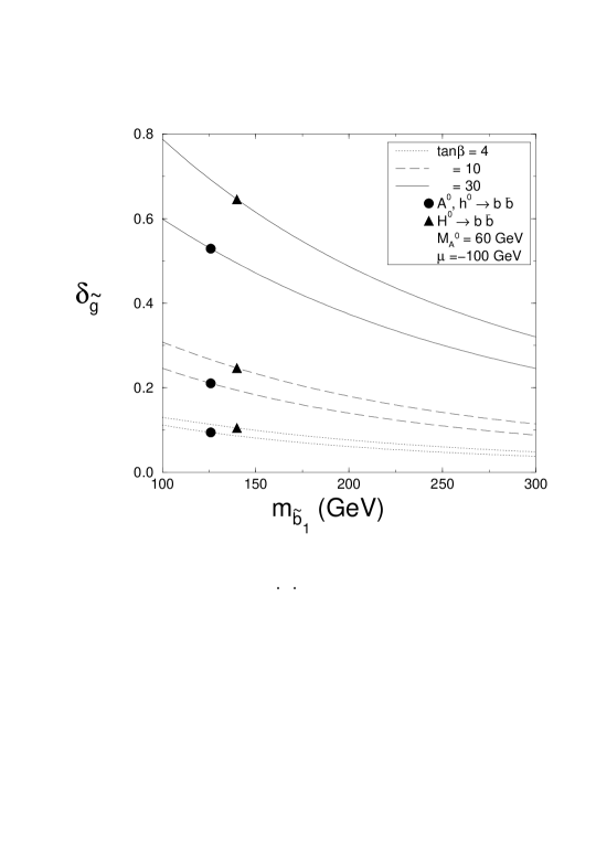
Figure 7: The sbottom–gluino QCD correction to the decays $h,H,A\rightarrow b\bar{b}$ normalized to the Born widths as a function of $m_{\tilde{b}_{1}}$ for various values of $\mbox{tg}\beta$ and fixed values of $\mu$ and $M_{A}$; taken from Ref. $\!{}^{{\bf?}}$.

For heavier Higgs bosons, the SUSY–QCD corrections to the decays $H,A\rightarrow t\bar{t}$ and $H^{+}\rightarrow t\bar{b}$ can also be large $\!{}^{{\bf?},{\bf?}}$, reaching the level of several 10%.

In the gluonic decay modes $h,H\rightarrow gg$, squark and in particular top squark loops must be included [squark loops do not contribute to the $Agg$ coupling because of CP–invariance] since these contributions are significant for squark masses $M_{\tilde{Q}}\raisebox{-3.69899pt}{~{}\shortstack{$<$ \\ [-0.07cm] $\sim$}}~{}500$ GeV and small $\mbox{tg}\beta$ values. This can be seen in Fig. 8 where the ratio of the gluonic decay width of the $h$ boson with and without the squark contributions is shown as a function $M_{\tilde{Q}}$ for $\mbox{tg}\beta=1.5,30$. The QCD corrections $\!{}^{{\bf?}}$ to the squark contribution have been calculated in the heavy squark mass limit, and are approximately of the same size as the the QCD corrections to the top quark contribution. A reasonable approximation [within about 10% ] to the gluonic decay width can be obtained by multiplying the full lowest order expression [including quark and squark contributions] with the relative QCD corrections including only quark loops.

Note that the QCD correction to the squark contribution to the $h\rightarrow\gamma\gamma$ coupling, which will be discussed later, has also been calculated $\!{}^{{\bf?}}$: in the heavy squark mass limit and relatively to the Born term, the correction is $8\alpha_{s}/3\pi$ [compared to $-\alpha_{s}/\pi$ for the top quark loop] and is therefore small.

Figure 8: Ratio of the QCD-corrected decay width $\Gamma(h\rightarrow gg)$ with and without squark loops for two values of $\mbox{tg}\beta=1.5,30$ as a function of the common squark mass $M_{\tilde{Q}}$. $M_{A}=100$ GeV and the second axes show the corresponding values of $M_{h}$; from Ref.$\!{}^{{\bf?}}$.

5.2 SUSY Loop Effects in $h\rightarrow\gamma\gamma$

In the decoupling limit, $M_{H}\sim M_{A}\sim M_{H^{+}}\gg M_{Z}$, the lightest SUSY Higgs boson $h$ has almost the same properties as the SM Higgs particle $H^{0}$ and the MSSM and SM Higgs sectors look practically the same. In the case where no genuine SUSY particle and no additional Higgs boson have been found at future machines, the task of discriminating between the lightest SUSY and the SM Higgs boson is challenging. A way to discriminate between the two in this decoupling regime is to look at loop induced Higgs boson couplings such as the couplings to $gg$, $Z\gamma$ and $\gamma\gamma$. In the SM, these couplings are mediated by heavy quark and $W$ boson loops [only quark loops for the $H^{0}gg$ coupling]. In supersymmetric theories, additional contributions will be induced by loops with charged Higgs bosons, charginos and sfermions.

The $hgg$ coupling, which can be measured in the decays $h\rightarrow gg$ or at the LHC in the dominant production mechanism $gg\rightarrow h$, has been discussed previously. The $hZ\gamma$ coupling, which could be measured for $M_{h}<M_{Z}$ in the decay $Z\rightarrow h\gamma$, at a high–luminosity $e^{+}e^{-}$ collider running at the Z–peak, or in the reverse decay $h\rightarrow Z\gamma$ if $M_{h}>M_{Z}$ at the LHC, has been discussed in Ref. $\!{}^{{\bf?}}$: the SUSY–loop effects are large only in extreme situations, and are unlikely to be seen in these decays. We will discuss here only the $h\gamma\gamma$ coupling $\!{}^{{\bf?}}$ which could be measured in the decays $h\rightarrow\gamma\gamma$ with the Higgs boson produced at LHC in the $gg\rightarrow h$ mechanism or at future high–energy and high–luminosity $e^{+}e^{-}$ colliders in the process $e^{+}e^{-}\rightarrow h\nu\bar{\nu}$, and most promising in the s–channel single Higgs production in the fusion process $\gamma\gamma\rightarrow h$, with the photons generated by Compton–back scattering of laser light [a measurement with a precision of the order of 10% could be feasible in this case].

The contributions of charged Higgs bosons, sleptons and the scalar partners of the light quarks including the bottom squarks are extremely small. This is due to the fact that these particles do not couple to the Higgs boson proportionally to the mass, and the amplitude is damped by inverse powers of the heavy mass squared; in addition, the couplings are small and the amplitude for spin–0 particles is much smaller than the dominant $W$ amplitude.

The contribution of the charginos to the two–photon decay width can exceed the 10% level for masses close to $m_{\chi}\sim 100$ GeV, but it becomes smaller with higher masses. The deviation of the $\Gamma(h\rightarrow\gamma\gamma)$ width from the SM value induced by charginos with masses $m_{\chi}=250$ and $400$ GeV is shown in Fig. 9, as a function of $M_{2}$ [$\mu$ is fixed by $m_{\chi}$] for $\mbox{tg}\beta=1.6$ and $50$. For chargino masses above $m_{\chi}\raisebox{-3.69899pt}{~{}\shortstack{$>$ \\ [-0.07cm] $\sim$}}~{}250$ GeV [i.e. slightly above the limit where charginos can be produced at e.g. a 500 GeV $e^{+}e^{-}$ collider], the deviation is less than $\sim 8\%$ for the entire SUSY parameter space. The deviation drops by a factor of two if the chargino mass is increased to 400 GeV.

Because its coupling to the lightest Higgs boson can be strongly enhanced, the top squark can generate sizeable contributions to the two–photon decay width of the $h$ boson. For stop masses in the $\sim 100$ GeV range, the contribution could reach the level of the dominant $W$ boson contribution and the interference is constructive increasing drastically the decay width. For $\tilde{t}_{1}$ masses around 250 GeV, the deviation of the $h\rightarrow\gamma\gamma$ decay width from the SM value can be still at the level of 10% for a very large off–diagonal entry in the stop mass matrix, $m^{LR}_{t}\raisebox{-3.69899pt}{~{}\shortstack{$>$ \\ [-0.07cm] $\sim$}}~{}1$ TeV; Fig. 9. For larger masses, the deviation drops $\sim 1/m_{\tilde{t}_{1}}^{2}$ and the effect on the decay width is below $2\%$ for $m_{\tilde{t}_{1}}\sim 400$ GeV even at $m^{LR}_{t}\sim 1$ TeV. For small values of $m^{LR}_{t}$, the deviation does not exceed $-8\%$ even for a light top squark $m_{\tilde{t}_{1}}\sim 250$ GeV.

Figure 9: The deviations of the SUSY Higgs coupling to two photons from the SM value [in %] for two values of $\mbox{tg}\beta=1.6$ and 50 and the loops masses $m_{i}=250$ and $400$ GeV. Deviations due to the chargino loops as a function of $M_{2}$ for both signs of $\mu$ (up), and deviations due to the top squark loops (down) as a function of $m_{t}^{LR}$; from Ref. $\!{}^{{\bf?}}$.

6 The program HDECAY

Finally, let me make some propaganda and shortly describe the fortran code HDECAY $\!{}^{{\bf?}}$, which calculates the various decay widths and the branching ratios of Higgs bosons in the SM and the MSSM and which includes:

(a) All decay channels that are kinematically allowed and which have branching ratios larger than $10^{-4}$, y compris the loop mediated, the three body decay modes and in the MSSM the cascade and the supersymmetric decay channels.

(b) All relevant two-loop QCD corrections to the decays into quark pairs and to the quark loop mediated decays into gluons are incorporated in the most complete form; the small leading electroweak corrections are also included.

(c) Double off–shell decays of the CP–even Higgs bosons into massive gauge bosons which then decay into four massless fermions, and all all important below–threshold three–body decays discussed previously.

(d) In the MSSM, the complete radiative corrections in the effective potential approach with full mixing in the stop/sbottom sectors; it uses the renormalisation group improved values of the Higgs masses and couplings and the relevant leading next–to–leading–order corrections are also implemented.

(e) In the MSSM, all the decays into SUSY particles (neutralinos, charginos, sleptons and squarks including mixing in the stop, sbottom and stau sectors) when they are kinematically allowed. The SUSY particles are also included in the loop mediated $\gamma\gamma$ and $gg$ decay channels.

The basic input parameters, fermion and gauge boson masses and total widths, coupling constants and in the MSSM, soft–SUSY breaking parameters can be chosen from an input file. In this file several flags allow to switch on/off or change some options [e.g. chose a particular Higgs boson, include/exclude the multi–body or SUSY decays, or include/exclude specific higher–order QCD corrections]. The results for the many decay branching ratios and the total decay widths are written to several output files with headers indicating the processes and giving the input parameters.

The program is written in FORTRAN and has been tested on several machines: VAX stations under the operating system VMS and work stations running under UNIX. All the necessary subroutines [e.g. for integration] are included. The program is lengthy [more than 5000 FORTRAN lines] but rather fast, especially if some options [as decays into double off-shell gauge bosons] are switched off.

7 Summary

In this talk, the decay modes of the Standard and Supersymmetric Higgs bosons in the MSSM, have been reviewed and updated. The relevant higher–order corrections which are dominated by the QCD radiative corrections and the off–shell [three–body] decays have been discussed. In the MSSM, the SUSY decay modes, and in particular the decays into charginos, neutralinos, and top squarks [as well as decays into light gravitinos] can be very important in large regions of the parameter space. The SUSY–loop contributions to the standard decays into quarks, gluons and photons of the MSSM Higgs bosons can also be important for not too heavy SUSY particles. The total decays widths of the Higgs bosons and the various branching ratios in the SM and in the MSSM, including the previous points can be obtained using the program HDECAY.

References

References

- [1] For a review on the Higgs sector of the SM and the MSSM , see J.F. Gunion, H.E. Haber, G.L. Kane and S. Dawson, The Higgs Hunters Guide, Addison-Wesley, Reading 1990.
- [2] For a review on Higgs physics at future hadron and colliders see e.g., A. Djouadi, Int. J. Mod. Phys. A10 (1995) 1.
- [3] P. Janot, EuroConference on High–Energy Physics, Jerusalem, 1997.
- [4] For a recent account on the constraints on the SM and MSSM Higgs masses, see M. Carena, P.M. Zerwas et al., Higgs Physics at LEP2, CERN 96–01, G. Altarelli, T. Sjöstrand and F. Zwirner (eds.).
- [5] Y. Okada, M. Yamaguchi and T. Yanagida, Prog. Theor. Phys. 85 (1991) 1; H. Haber and R. Hempfling, Phys. Rev. Lett. 66 (1991) 1815; J. Ellis, G. Ridolfi and F. Zwirner, Phys. Lett. B257 (1991) 83; R. Barbieri, F. Caravaglios and M. Frigeni, Phys. Lett. B258 (1991) 167; A. Hoang and R. Hempfling, Phys. Lett. B331 (1994) 99; J. Casas, J. Espinosa, M. Quiros and A. Riotto, Nucl. Phys. B436 (1995) 3; M. Carena, J. Espinosa, M. Quiros and C.E.M. Wagner, Phys. Lett. B355 (1995) 209.
- [6] See the talk given by M. Quiros, these proceedings.
- [7] M. Spira, Report CERN-TH/97-68, hep-ph/9705337.
- [8] See the talk given by W. Hollik at this Workshop, hep-ph/9711489, to appear in the proceedings.
- [9] For an update of the effect of QCD corrections to the hadronic decay widths, see A. Djouadi, M. Spira and P.M. Zerwas, Z. Phys. C70 (1996) 427; see also J. Kamoshita, Y. Okada and M. Tanaka, Phys. Lett. B391 (1997) 124; and Z. Kunszt, S. Moretti and W.J. Stirling Z. Phys. C74 (1997) 479.
- [10] E. Braaten and J.P. Leveille, Phys. Rev. D22 (1980) 715; M. Drees and K. Hikasa, Phys. Lett. B240 (1990) 455; (E) B262 (1991) 497.
- [11] S.G. Gorishny, A.L. Kataev, S.A. Larin and L.R. Surguladze, Mod. Phys. Lett. A5 (1990) 2703; Phys. Rev. D43 (1991) 1633; A.L. Kataev and V.T. Kim, Mod. Phys. Lett. A9 (1994) 1309; L.R. Surguladze, Phys. Lett. 341 (1994) 61; K.G. Chetyrkin, Phys. Lett. B390 (1997) 309.
- [12] N. Gray, D.J. Broadhurst, W. Grafe and K. Schilcher, Z. Phys. C48 (1990) 673.
- [13] S. Narison, Phys. Lett. B341 (1994) 73.
- [14] S.G. Gorishny, A.L. Kataev, S.A. Larin and L.R. Surguladze, Mod. Phys. Lett. A5 (1990) 2703; Phys. Rev. D43 (1991) 1633
- [15] R. Harlander and M. Steinhauser, Phys. Rev. D56 (1997) 3980.
- [16] The discussions on the three-body decays are based on: A. Djouadi, J. Kalinowski and P.M. Zerwas, Z. Phys. C70 (1996) 437; see also S. Moretti and W.J. Stirling, Phys. Lett. B347 (1995) 291; (E) B366 (1996) 451.
- [17] For a summary and a complete set of references, see B.A. Kniehl, Phys, Rep. 240 (1994) 211.
- [18] J. Ellis, M.K. Gaillard and D.V. Nanopoulos, Nucl. Phys. B106 (1976) 292; A.I. Vainshtein, M.B. Voloshin, V.I. Sakharov and M.A. Shifman, Sov. J. Nucl. Phys. 30 (1979) 711.
- [19] M. Spira, A. Djouadi, D. Graudenz and P.M. Zerwas, Nucl. Phys. B453 (1995) 17.
- [20] T. Inami, T. Kubota and Y. Okada, Z. Phys. C18 (1983) 69; A. Djouadi, M. Spira and P.M. Zerwas, Phys. Lett. B264 (1991) 440.
- [21] K.G. Chetyrkin, B.A. Kniehl and M. Steinhauser, Phys. Rev. Lett. 79 (1997) 353.
- [22] B.W. Lee, C. Quigg and H.B. Thacker, Phys. Rev. D16 (1977) 1519.
- [23] A. Ghinculov, Nucl. Phys. B455 (1995) 21; A. Frink, B. Kniehl, D. Kreimer, and K. Riesselmann, Phys. Rev. D54 (1996) 4548.
- [24] T.G. Rizzo, Phys. Rev. D22 (1980) 389; W.-Y. Keung and W.J. Marciano, Phys. Rev. D30 (1984) 248.
- [25] See e.g., R.N. Cahn, Rep. Prog. Phys. 52 (1989) 389.
- [26] A. Mendez and A. Pomarol, Phys. Lett. B252 (1990) 461; C.S. Li and R.J. Oakes, Phys. Rev. D43 (1991) 855; A. Djouadi and P. Gambino, Phys. Rev. D51 (1995) 218.
- [27] J.F. Gunion and H. Haber, Phys. Rev. D48 (1993) 5109; G. L. Kane, G. D. Kribs, S. P. Martin and J. D. Wells, Phys. Rev. D53 (1996) 213; B. Kileng, P. Osland and P.N. Pandita, Z. Phys. C71 (1996) 87.
- [28] S. Heinemeyer and W. Hollik, Nucl. Phys. B474 (1996) 32.
- [29] J.F. Gunion and H.E. Haber, Nucl. Phys. B272 (1986) 1; B278 (1986) 449; B307 (1988) 445; (E) hep-ph/9301201.
- [30] A. Djouadi, P. Janot, J. Kalinowski and P.M. Zerwas, Phys. Lett. B376 (1996) 220; A. Djouadi, J. Kalinowski and P.M. Zerwas, Z. Phys. C57 (1993) 569.
- [31] A. Djouadi, J. Kalinowski, P. Ohmann and P.M. Zerwas, Z. Phys. C74 (1997) 93.
- [32] J.F. Gunion and H.E. Haber, Phys. Rev. D37 (1988) 2515; A. Bartl et al., Phys. Lett. B373 (1996) 117.
- [33] J. Ellis and D. Rudaz, Phys. Lett. B128 (1983) 248; K. Hikasa and M. Drees, Phys. Lett. B252 (1990) 127.
- [34] A. Bartl, H. Eberl, K. Hidaka, T. Kon, W. Majerotto and Y. Yamada, Report UWThPh-1997-03, hep-ph/9701398; A. Arhrib, A. Djouadi, W. Hollik and C. Jünger, Report KA-TP-30-96, hep-ph/9702426; see also the talks of A. Bartl and W. Majerotto in these proceedings.
- [35] P. Fayet, Phys. Lett. 70B, 461 (1977) and B175, 471 (1986).
- [36] S. Ambrosiano, G.L. Kane, G.D. Kribs, S.P. Martin and S. Mrenna, Phys. Rev. D54, 5395 (1996); J. Ellis, J.L. Lopez and D.V. Nanopoulos, Phys. Lett. B394 (1997) 354.
- [37] A. Djouadi and M. Drees, Phys. Lett. B407 (1997) 243.
- [38] C.S. Li and J.M. Yang, Phys. Lett. B315 (1993) 367; A. Dabelstein, Nucl. Phys. B456 (1995) 25; A. Bartl, H. Eberl, K. Hidaka, T. Kon, W. Majerotto and Y. Yamada Phys. Lett. B378 (1996) 167; R.A. Jimenez and J. Sola, Phys. Lett. B389 (1996) 53; see also the talk of W. Majerotto in these proceedings.
- [39] J.A. Coarasa, R.A. Jimenez and J. Solà, Phys. Lett. B389 (1996) 312.
- [40] A. Dabelstein and W. Hollik, Report MPI-PH-93-86; see also the talk by W. Hollik, these proceedings.
- [41] S. Dawson, A. Djouadi and M. Spira, Phys. Rev. Lett. 77 (1996) 16.
- [42] A. Djouadi, V. Driesen, W. Hollik and J.I. Illana, hep-ph/9612362.
- [43] A. Djouadi, V. Driesen, W. Hollik and A. Kraft, hep-ph/9701342.
- [44] A. Djouadi, J. Kalinowski and M. Spira, hep-ph/9704448; the program can be obtained from the net at http://www.lpm.univ-montp2.fr/djouadi/program.html or http://wwwcn.cern.ch/mspira.