IASSNS-HEP-97/68

CERN-TH/97-292

hep-ph/9712322

December 1997

Twenty Open Questions
in Supersymmetric Particle Physics
Keith R. Dienes^1,2  and  Christopher Kolda^1
1 School of Natural Sciences, Institute for Advanced Study
Olden Lane, Princeton, N.J.  08540  USA
² CERN Theory Division, CH-1211 Geneva 23, Switzerland

We give a brief overview of 20 open theoretical questions in supersymmetric particle physics. The 20 questions we have chosen range from the GeV scale to the Planck scale, and include issues pertaining to the Minimal Supersymmetric Standard Model and its extensions, SUSY-breaking, cosmology, grand unified theories, and string theory. Throughout, our goal is to address those topics in which supersymmetry plays a fundamental role, and which are areas of active research in the field. This survey is written at an introductory level and is aimed at people who are not necessarily experts in the field.

At first glance, supersymmetry appears to be a theoretical success story writ large. With one simple idea, such diverse issues as extending the Lorentz group, solving the gauge hierarchy problem, coupling gauge theories to gravity, and generating gauge coupling unification all seem to fall into place. The lack of direct experimental evidence for supersymmetry (SUSY) dampens our enthusiasm somewhat, but only now (and over the next few years) are experiments really beginning to probe the domain where SUSY should be expected to be manifest.

Nonetheless, there is a price to be paid for the successes of SUSY, and we mean more than simply the doubling of the Standard Model (SM) particle spectrum. SUSY introduces into physics a host of new questions which must be addressed, and hopefully, answered. Most of these questions were once real problems — problems which seemed to detract from, or perhaps even invalidate, SUSY as a viable fundamental symmetry of nature. Although some of the questions presented here do not have attractive solutions, none of them, nor any others that we are aware of, threaten to rule out SUSY. Instead, as competing answers to these questions have been found, these questions become opportunities not only to simply discover SUSY, but also to probe physics well beyond the scale of SUSY.

The questions that we will consider in this work have been chosen because they satisfy a number of important criteria. First and foremost, each defines an area of active research in the field; in many ways, the list of questions that follows forms a summary of current topics of interest in applying SUSY to the physics of the SM.

Second, these are questions which are intrinsically supersymmetric and may not even arise in the SM alone. Thus, generic questions in the SM (such as the cosmological constant, inflation, baryogenesis, and fermion mass hierarchies, to name a few) are not included here. This is not to say that SUSY does not have implications for these subjects, for it usually does, and when it does it typically recasts the terms of the debate completely by redefining the spectrum of possible solutions. However, in this article we will concentrate on those issues which are intrinsically supersymmetric and whose solutions one would hope to find in a complete description of a supersymmetric SM. After all, it would be wonderful if SUSY could explain why the electron is so much lighter than the top quark, but there is no obvious reason to suppose that it will since the question itself is intrinsically non-supersymmetric.

Third, these are questions whose answers may tell us a great deal about physics beyond the MSSM, yet which might be probed using only a combination of experimental measurements of the MSSM and theoretical constraints. In this sense, these questions are windows through which insight far beyond the weak scale may be sought.

Because we focus primarily on questions that have direct applicability to the physics of the SM or MSSM, a large number of interesting topics will receive only abbreviated attention. For example, recent results on the dynamics of SUSY gauge theories may have profound effects on how we approach the MSSM in coming years (as they already have had on the question of SUSY-breaking), but their current applications are limited. Thus we will only touch upon this and related topics of a more formal nature.

The open questions we have chosen to address are as follows. First, at the lowest energy scales, we have selected a number of open questions that pertain to the MSSM itself:

• Question #1:   Why doesn’t the proton decay in $10^{-17}$ years?

• Question #2:   How is flavor-changing suppressed?

• Question #3:   Why isn’t CP violation ubiquitous?

• Question #4:   Where does the $\mu$-term come from?

• Question #5:   Why does the MSSM conserve color and charge?

Next, we consider open questions pertaining to SUSY-breaking:

• Question #6:   How is SUSY broken?

• Question #7:   Once SUSY is broken, how do we find out?

Then, we consider two open questions pertaining to natural extensions of the MSSM:

• Question #8:   Can singlets and SUSY coexist?

• Question #9:   How do extra $U(1)$’s fit into SUSY?

Our next set of open questions addresses the interplay between supersymmetry and cosmological issues:

• Question #10:   How does SUSY shed light on dark matter?

• Question #11:   Are gravitinos dangerous to cosmology?

• Question #12:   Are moduli cosmologically dangerous?

We then turn our attention to supersymmetric GUT’s:

• Question #13:   Does the MSSM unify into a SUSY GUT?

• Question #14:   Proton decay again: Why doesn’t the proton decay in $10^{32}$ Question #14:     years?

• Question #15:   Can SUSY GUT’s explain the masses of fermions?

Next, we discuss some recent formal developments concerning SUSY and gauge theory:

• Question #16:   N=1 SUSY duality: How has SUSY changed our view of gauge Question #17:    theory?

Finally, our last set of questions addresses supersymmetry at the very highest scales, in the context of string theory:

• Question #17:   Why strings?

• Question #18:   What roles does SUSY play in string theory?

• Question #19:   How is SUSY broken in string theory?

• Question #20:   Making ends meet: How can we understand gauge coupling Question #21:    unification from string theory?

Finally, many of the topics that we shall discuss here will be covered in much greater detail in the topical chapters of this book, and we will try to indicate the relevant chapters as we go along.

  

Section I:   Open Questions in the MSSM

The Standard Model forms the bedrock of modern high-energy physics, and accurately describes all physical phenomena down to scales of $10^{-16}$ cm. However, there are many possible ways of extending the SM down to smaller length scales. These include extra gauge interactions, new matter, new levels of compositeness (technicolor), and supersymmetry. While supersymmetry does not succeed as an explanation of the features of the SM, it provides a remarkably robust extension to the SM which is in agreement with all experimental data. This cannot be said for many other possible extensions (such as, e.g., the simplest versions of technicolor). Moreover, it is quite possible and perhaps even likely that other forms of potential new physics might appear at the same energy scale as supersymmetry. Thus, as a first step, it is important to investigate how the structure of supersymmetry might be joined with that of the SM in a cohesive framework.

Although there are various ways in which SUSY might be joined with the SM, for simplicity one can pursue a minimal construction, and attempt to write down a Lagrangian which is the most general effective Lagrangian for the minimal extension of the SM which is invariant under SUSY transformations up to soft-breaking terms. This then results in the Lagrangian of the Minimal Supersymmetric Standard Model (MSSM). We will not attempt to fully define the MSSM, its field content, or its Lagrangian, but instead we refer the reader to any of several standard references [1], or to the article of S. Martin in this volume. We will therefore say only a few words of a general nature.

The minimal extension of the SM with unbroken SUSY is a simple model with fewer free parameters than the SM itself, despite the large number of new fields. It is only in the breaking of SUSY that the number of free parameters becomes large — but of course, it is only in the breaking of SUSY that the model can even attempt to describe nature as we observe it. In the SM, the field content along with the gauge symmetries serve to provide a number of accidental symmetries at the renormalizable level. These include, for example, baryon number $B$, and lepton number $L$. These symmetries also serve to forbid flavor-changing neutral currents (FCNC’s) up to small corrections arising from Yukawa couplings in loops. The MSSM shares neither of these properties. As we will discuss, the most general MSSM would have the proton decay with a weak-interaction lifetime and large FCNC’s. The reason is this same proliferation of fields and free parameters. Even after imposing symmetries to forbid the fast proton decay (see Question #1 below), one finds [2] that the MSSM contains 106 new, independent (real) parameters above and beyond those of the SM. These consist of 26 masses (resulting from 12 squark, 9 slepton, and 3 gaugino masses, plus $\mu$- and $B_{\mu}$-terms), 37 mixing angles, and 43 CP-violating phases. Understanding, constraining, and ultimately measuring these parameters is one of the primary goals of the SUSY program in particle physics.

Of course, the MSSM is unlikely to be the end of the story. Therefore, although we will begin this article by considering open questions within the MSSM, we will later allow this structure to expand by considering new singlets, extra gauge symmetries, grand unification, and ultimately embeddings within string theory.

One recurring feature in many of the open questions in this article is the question of “naturalness”: why is some coupling (or mass) very small or even zero when it need not have been zero a priori? More precisely, this is a question of “Dirac naturalness.” The idea of Dirac naturalness is built on the supposition that in any physical system, all couplings and interactions which are not otherwise forbidden should be allowed, and that all ratios of couplings, as well as all ratios of masses, should be ${\cal O}(1)$. We generally find that a theory is Dirac natural if some exact symmetry exists which forbids the undesired couplings. Note that Dirac naturalness is not to be confused with “’t Hooft naturalness” or “technical naturalness,” which is the problem besetting the Higgs sector of the Standard Model. In the latter case one seeks to understand small numbers or ratios, such as the ratio of the weak to Planck scale, in terms of approximate symmetries. The role of radiative corrections is very important for ’t Hooft naturalness, because even if one could choose the ratio of two couplings or two masses to be far from unity at tree level, without some approximate symmetry at play there would be no reason for this ratio to persist beyond tree level. The chiral symmetry of the SM fermions is a classic example of this phenomenon: an approximate symmetry protects the fermion masses from receiving corrections proportional to heavy mass scales.

Without SUSY, there is nothing like a chiral symmetry to protect scalar masses from heavy mass scales. But with SUSY, the chiral symmetry in the fermionic sector protects the scalars too. This is a general feature of SUSY — couplings and masses which are SUSY-preserving are automatically natural à la ’t Hooft even if they are unnatural à la Dirac. Thus when we speak of naturalness in the context of SUSY, we will generally be referring to Dirac naturalness, for which SUSY provides no automatic solutions.

Question #1   Why doesn’t the proton decay in $10^{-17}$ years?

As discussed in the article of S. Martin in this volume, the most general, renormalizable superpotential for the MSSM can be organized into three pieces, $W=W_{0}+W_{B\!\!\!\!/}+W_{L\!\!\!/}$, where

$$W_{0} = y^{U}_{ij}Q^{i}u^{j}H_{U}+y^{D}_{ij}Q^{i}d^{j}H_{D}+y^{E}_{ij}L^{i}e^{j}H_{D}+\mu H_{U}H_{D}$$ (1)

$$W_{L\!\!\!/} = \lambda_{ijk}Q^{i}d^{j}L^{k}+\lambda^{\prime}_{ijk}e^{i}L^{j}L^{k}+\mu^{\prime}_{i}H_{U}L^{i}$$ (2)

$$W_{B\!\!\!\!/} = \lambda^{\prime\prime}_{ijk}u^{i}d^{j}d^{k}~{}.$$ (3)

The first piece preserves the global $B$ and $L$ quantum numbers of the SM, while the other two each violate one of either $B$ or $L$. This is to be contrasted with the case of the SM in which one can obtain $B$-violating operators only by going to dimension six, or $L$-violating operators only by going to dimension five. Allowing simultaneous $B$- and $L$-violation would be a disaster. For example, given non-zero $\lambda$ and $\lambda^{\prime\prime}$, one can form a four-fermion operator $QudL$ which can mediate proton decay and is only suppressed by squark masses [3, 4], not $M_{\rm GUT}$ or $M_{\rm Pl}$.

There is a simple remedy for this: one can set $W_{B\!\!\!\!/}=W_{L\!\!\!/}=0$ by hand. In a non-supersymmetric theory, this would be ’t Hooft unnatural unless there existed some exact global or gauge symmetry to ensure that these couplings remain zero. In a supersymmetric theory, however, couplings in the superpotential are always ’t Hooft natural due to the “non-renormalization” theorem, which says that any couplings in $W$ that are set to zero will remain zero to orders in perturbation theory. Nonetheless, setting otherwise-allowed couplings to zero is always Dirac unnatural and so we might look for a symmetry that arises when these couplings vanish. The obvious candidates, global $B$ and $L$ symmetries, are probably not suitable to play this role since we expect from a number of arguments (e.g., involving GUT’s, $\nu$ masses, cosmological baryon asymmetry) that they will be broken by non-renormalizable or non-perturbative terms.

Fortunately it is easy to invent a new discrete symmetry which simultaneously forbids all the unwanted terms and which allows those that are phenomenologically necessary. This is “matter parity,” a $\mathchoice{\hbox{\cmss Z\kern-3.99994ptZ}}{\hbox{\cmss Z\kern-3.99994ptZ}}{\lower 0.9pt\hbox{\cmsss Z\kern-2.79996ptZ}}{\lower 1.2pt\hbox{\cmsss Z\kern-2.79996ptZ}}_{2}$ symmetry under which all the matter fields $(L,e,Q,u,d)$ are odd and the Higgs fields are even [5]. An added benefit of such a symmetry is the exact stability of the lightest supersymmetric particle (LSP), even against higher-order interactions, thereby providing a candidate for the (cold) dark matter in the universe.

Though matter parity may provide a “Dirac natural” solution to the proton decay problem, there is a more recent definition of naturalness which matter parity does not necessarily satisfy. We shall refer to this new definition, which comes out of ideas in string theory and quantum gravity, as “local naturalness.” Whereas Dirac naturalness would allow any exact global symmetry to forbid the unwanted couplings, local naturalness requires that these symmetries be gauge symmetries, or at least the indirect consequence of an underlying gauge symmetry [6]. This requirement follows from the result/belief that in a theory of quantum gravity, there may be effects (potentially arising from Planck-scale physics) which violate any and all symmetries of the theory which are not gauged or somehow protected by a gauge symmetry. These protected symmetries include global and discrete subgroups of gauge symmetries. And though these Planck-scale effects might be small, suppressed by powers of $M_{\rm Pl}$, in some cases this may be enough to violate known constraints. In the case of proton decay, such a violation occurs. It would be desirable, then, to embed matter parity into a gauge symmetry.

In order to see how this might be done, note that the matter parity $P_{M}$ of any MSSM field with baryon and lepton numbers $B$ and $L$ respectively can be written as

$$P_{M}=(-1)^{3(B-L)}.$$ (4)

Matter parity can therefore easily be accommodated as a discrete subgroup of a gauged $U(1)_{B-L}$ symmetry, something which appears in many extensions of the SM. In fact, the action of the full $U(1)_{B-L}$ symmetry would be to forbid exactly the unwanted terms in $W$. If this selection rule is to survive the breakdown of the $U(1)_{B-L}$ symmetry, then one need only require that all order parameters (e.g., Higgs VEV’s) carry even integer values of $3(B-L)$. This restriction can also be generalized to groups containing $U(1)_{B-L}$; for example, in $SO(10)$ one finds [7] that matter parity occurs as a discrete gauge symmetry after GUT-breaking if that breaking is done without giving VEV’s to spinor representations (e.g., ${\bf 16,144,560}\ldots$).

The question of how one can embed such a discrete symmetry into a gauge symmetry can be further generalized by asking whether or not the set of discrete charges in the MSSM is “anomaly-free,” i.e., whether or not these charges obey certain constraints which allow them to be interpreted as arising from a non-anomalous gauge symmetry (as in the example above). One can in fact show that matter parity is the only (generation-independent) $\mathchoice{\hbox{\cmss Z\kern-3.99994ptZ}}{\hbox{\cmss Z\kern-3.99994ptZ}}{\lower 0.9pt\hbox{\cmsss Z\kern-2.79996ptZ}}{\lower 1.2pt\hbox{\cmsss Z\kern-2.79996ptZ}}_{2}$ symmetry which is anomaly-free and prevents dimension-four proton decay [8].

Of course, the original argument against allowing non-zero $W_{B\!\!\!\!/}$ and $W_{L\!\!\!/}$ was that both could not be allowed without leading to rapid nucleon decay. This argument suffices to forbid one or the other, but not both. In fact, much work has been done considering extensions of the MSSM with so-called “$R$-parity violation” in which either $W_{B\!\!\!\!/}$ or $W_{L\!\!\!/}$ is non-zero, but not both. The price one pays is that the LSP is no longer stable and so there is no easy candidate for the dark matter. However, the phenomenology and motivations of $R$-parity violation are too complicated to discuss here; for details, see the contribution of H. Dreiner to this volume.

Thus far, we have said nothing about proton decay from higher-dimension operators. In particular there are many terms of dimension five which are invariant under matter parity which can mediate proton decay. For example, let us consider the superpotential term $W=(\frac{\eta}{M})QQQL$. Even if one identifies $M$ with the Planck mass, current bounds on the proton lifetime require that $\eta$ be unnaturally small: $\eta\lower 3.01385pt\hbox{$\;\stackrel{{\scriptstyle\textstyle<}}{{\sim}}\;$}10^{-7}$. One could consider alternative $\mathchoice{\hbox{\cmss Z\kern-3.99994ptZ}}{\hbox{\cmss Z\kern-3.99994ptZ}}{\lower 0.9pt\hbox{\cmsss Z\kern-2.79996ptZ}}{\lower 1.2pt\hbox{\cmsss Z\kern-2.79996ptZ}}_{N}$ symmetries for the superpotential, and in fact one particular alternative [8] stands out: a $\mathchoice{\hbox{\cmss Z\kern-3.99994ptZ}}{\hbox{\cmss Z\kern-3.99994ptZ}}{\lower 0.9pt\hbox{\cmsss Z\kern-2.79996ptZ}}{\lower 1.2pt\hbox{\cmsss Z\kern-2.79996ptZ}}_{3}$ symmetry called “baryon parity.” Under baryon parity the MSSM fields $({\widetilde{Q}},{\widetilde{u}},{\widetilde{d}},{\widetilde{L}},{\widetilde{e}},H_{U},H_{D})$ have $\mathchoice{\hbox{\cmss Z\kern-3.99994ptZ}}{\hbox{\cmss Z\kern-3.99994ptZ}}{\lower 0.9pt\hbox{\cmsss Z\kern-2.79996ptZ}}{\lower 1.2pt\hbox{\cmsss Z\kern-2.79996ptZ}}_{3}$ charges (0,2,1,2,2,1,2) respectively. Baryon parity has many interesting properties: it is the only (generation-independent) $\mathchoice{\hbox{\cmss Z\kern-3.99994ptZ}}{\hbox{\cmss Z\kern-3.99994ptZ}}{\lower 0.9pt\hbox{\cmsss Z\kern-2.79996ptZ}}{\lower 1.2pt\hbox{\cmsss Z\kern-2.79996ptZ}}_{3}$ symmetry of the MSSM without discrete gauge anomalies; it prevents dimension-four proton decay by forbidding $W_{B\!\!\!\!/}$; it allows the $\mu$-term; it allows $W_{L\!\!\!/}$ and therefore neutrino masses; it forbids dimension-five proton decay; but it also allows the decay of the LSP.

Is matter parity, or any of its competitors, a real symmetry of nature? This is essentially an experimental question, but its implications go far beyond questions of detection signals, for these symmetries teach us about dark matter and the ultimate fate of the universe, and also provide insights into the symmetry structure of the MSSM at very high energies.

Question #2   How is flavor-changing suppressed?

There is no reason to expect that the mass and interaction eigenstates of the SM fermions coincide; that is, the quark and lepton mass matrices need not be diagonal in the interaction eigenbasis. In fact we know that they are not diagonal (since $\theta_{c}\neq 0$). One obviously expects the same to be true of the scalars of the MSSM. But before SUSY-breaking, one can expect that at least the mass matrices of fermions and their scalar superpartners will be diagonal in the same basis. This need not be true after SUSY-breaking.

In the interaction basis, non-diagonal mass matrices would seem to lead to large flavor-changing neutral currents (FCNC’s). Within the SM, it is the GIM mechanism which prevents this from occurring. Flavor-independent neutral current (NC) gauge interactions couple gauge bosons to propagating fermions and their conjugates, each rotated from their interaction basis by matrices $U$ and $U^{\dagger}$ respectively. As long as $U$ is unitary, then $U^{\dagger}U={\bf 1}$ and the NC gauge interaction conserves flavor. The same holds for the scalar partners which are rotated by unitary $\widetilde{U}$ and $\widetilde{U}^{\dagger}$. Thus gauge bosons do not induce FCNC’s for particles or their superpartners. The Problem arises with gauginos, which couple to both a particle and its superpartner simultaneously. In this case the coupling has the form $\widetilde{U}^{\dagger}U$, which need not be diagonal. Thus gauginos can generate FCNC’s [3, 9]. (This is not a complete disaster because for flavor-changing processes involving only fermions on external lines, gaugino contribution can arise only beyond the tree-level.)

Because FCNC’s are suppressed by GIM in the SM, the dominant source for FCNC’s in low-energy processes may come from SUSY. The tightest bounds on FCNC’s presently come from $K^{0}-\overline{K^{0}}$ mixing. Requiring that the MSSM prediction for the $K^{0}-\overline{K^{0}}$ mass difference not exceed the measured value yields limits of the form [11]:

$$\frac{{\cal A}^{2}}{m^{2}_{\widetilde{Q}}}\left(\frac{\delta m^{2}_{\widetilde{Q}}}{m^{2}_{\widetilde{Q}}}\right)^{2}~{}\leq~{}5\times 10^{-9}\,\,\mbox{GeV}^{-2}$$ (5)

where ${\cal A}^{2}$ is a product of angles which rotate from the quark mass basis to the squark mass basis, and $\delta m^{2}_{\widetilde{Q}}$ is the mass difference between the $\widetilde{d_{L}}$ and $\widetilde{s_{L}}$ squarks. There are corresponding limits on $\widetilde{d_{R}}-\widetilde{s_{R}}$ splittings as well as mixed left-right limits.

Given the above constraint, it is clear that if the mass splittings are ${\cal O}(1)$ and the angles take average values (${\cal A}^{2}\sim 1/20$), the squark mass scale must be $\lower 3.01385pt\hbox{$\;\stackrel{{\scriptstyle\textstyle>}}{{\sim}}\;$}3\,\mbox{TeV}$. Similar bounds exist from $D^{0}-\overline{D^{0}}$ and $B^{0}-\overline{B^{0}}$ mixing, and in the slepton sector from processes such as $\mu\to e\gamma$. However it is worth noting that bounds on FCNC’s tend to constrain only the first two generations of squarks and sleptons; the third generation is rather weakly constrained at present.

There are three primary proposals for solving the SUSY flavor problem: degeneracy, alignment, and decoupling.

Degeneracy attempts to solve the flavor problem by positing that squarks and sleptons of a given flavor are mass-degenerate [10, 11], i.e., $\delta m^{2}_{\widetilde{Q}}=0$. (One way to see that this would forbid FCNC’s is to note that if, for example, the $\widetilde{d}$ and $\widetilde{s}$ were to have equal mass, they would exactly cancel each other’s contributions to any flavor-changing process.) This extension of the GIM mechanism to the SUSY sector is often referred to as “super-GIM”: $m^{2}_{\widetilde{u}}=m^{2}_{\widetilde{c}}\simeq m^{2}_{\widetilde{t}}$ for L,R squarks separately, likewise $m^{2}_{\widetilde{e}}=m^{2}_{\widetilde{\mu}}\simeq m^{2}_{\widetilde{\tau}}$. Given the weaker bounds on FCNC’s involving the third generation, the final equalities need only be approximate.

Degeneracy models come in a variety of flavors themselves (for more details see Question #7). For many years, models based on supergravity (SUGRA) as a mediator of SUSY-breaking were considered members of this family. Now it is understood that there exist a number of rather generic phenomena which break degeneracy in SUGRA models, including non-minimal Kähler potentials, GUT effects, and superstring thresholds. Even if all of these could be ruled out, it is important to realize that sources of flavor physics between the Planck and weak scales tend to violate the degeneracy. This is a generic feature: if flavor physics occurs below the scale at which SUSY-breaking is communicated to the SM, scalar mass degeneracies will tend to be spoiled. An alternative to SUGRA mediation is gauge-mediated SUSY-breaking (GMSB). In GMSB two important things happen: the scalars of the MSSM receive their soft masses from SM gauge interactions, which are by definition flavor-universal, and these masses are communicated at scales often very close to the weak scale so that there is little room for new physics to spoil the degeneracy. Finally it has also been suggested that the flavor physics itself arises from non-abelian global symmetries (“horizontal” symmetries) under which the families of the SM/MSSM form non-trivial representations. These models usually predict some combination of degeneracy among the flavors and alignment, the next mechanism. One perhaps noteworthy aspect of non-abelian horizontal symmetries is that they can be gauged only in special cases [13], because the broken Cartan generators of a local symmetry typically generate $D$-terms which destroy the mass degeneracy that one worked so hard to obtain in the first place.

Alignment solves the flavor problem not by setting $\delta\widetilde{m}^{2}=0$ as with degeneracy, but by enforcing $U=\widetilde{U}$ (or equivalently ${\cal A}=0$) to a very high accuracy [12]. Here the flavor physics is typically generated by one or more $U(1)$ gauge interactions. Models of abelian horizontal symmetries seek to tie the generation of the scalar soft masses to that of the fermion mass/Yukawa matrices. All of these models generate the hierarchies in the fermion masses as powers of a small expansion parameter, usually the ratio between some flavor-violating VEV’s and the UV scale of the theory. Particularly interesting among these models are those in which the flavor $U(1)$ is pseudo-anomalous [14] — the anomalies in its fermionic sector are cancelled by non-linear transformations of the dilaton/axion superfield as in the Green-Schwarz mechanism of string theory. Such a $U(1)$ must be broken just below the string scale via a one-loop induced Fayet-Iliopoulos term, and it is the ratio of this breaking scale to the string scale that provides the expansion parameter for building the mass hierarchies.

Finally, decoupling has been proposed as a solution to the flavor problem [15]. Here one simply makes the first two generations of sparticles heavy enough (typically $10-100\,\mbox{TeV}$) so that their contributions to FCNC processes vanish. But what about the ’t Hooft naturalness problem in the SM Higgs sector that SUSY can solve only if the superpartners are light ($\lower 3.01385pt\hbox{$\;\stackrel{{\scriptstyle\textstyle<}}{{\sim}}\;$}1\,\mbox{TeV}$)? Recall that the troublesome diagrams involving scalars were all suppressed by Yukawa couplings. If we make the reasonable assumption that naturalness requires the gauginos, higgsinos, and the third generation of squarks and sleptons to lie below $1\,\mbox{TeV}$, then all the other squarks and sleptons can have masses as large as $(m_{t}/m_{q,\ell})\times(1\,\mbox{TeV})$ without violating naturalness constraints. (Here $m_{q,\ell}$ is the appropriate partner quark/lepton mass.) Once again one takes advantage of the fact that the bounds on third generation FCNC’s are weak in order to allow large mass splittings between the third generation and the first two. One should note, however, that there exist problems with the behavior of the decoupling scenario at two-loop order [16]; it is not clear at present that such a scenario can be made to work without inadvertently breaking QCD and/or QED.

Once SUSY is discovered, it may not take long to discern which of these paths nature has chosen to follow. Observation of scalar partners should quickly tell us whether they are degenerate or not (i.e., super-GIM or aligned); likewise, if only the third generation is found, we learn that the other spartners must be very heavy (i.e., decoupled). However, it will take much more experimental and theoretical work to determine just how each of these choices is concretely realized.

Question #3   Why isn’t CP violation ubiquitous?

In the MSSM there are 43 physical CP-violating phases above and beyond that of the SM. (In this discussion, we will ignore $\theta_{\rm QCD}$.) Unlike the single SM phase, which does not typically engender large CP-violating effects because in physical processes it always comes in proportional to the small Jarlskog parameter $J$, the phases of the MSSM can show up in large, easily observed, and easily constrained experimental processes. The tightest constraints come from CP-violating in the kaon system and the electric dipole moment of the neutron. The former receives SUSY contributions only if there are also flavor-changing SUSY contributions such as those discussed above; the latter exists even if SUSY is flavor-preserving. (For a review, see Ref. [17] and the contribution of A. Masiero and L. Silvestrini to this volume.)

Let us consider the second case first, with all SUSY flavor-changing effects put to zero through universal soft masses. For simplicity let us make the usual assumption that the trilinear couplings are all proportional to the Yukawas, and that the gaugino masses are universal at some scale. Then there remain only two physical phases beyond the SM associated with some combination of the $\mu$-term, the $B_{\mu}$-term, the $A$-terms, and the gaugino masses:

$$\phi_{A}=\arg(A^{*}M_{3})\quad\quad\quad\quad\phi_{B}=\arg(B_{\mu}^{*}\mu M_{3}).$$ (6)

At one-loop order, gluinos and squarks can contribute to the electric dipole moment (EDM) of quarks, and then in turn nuclei. The EDM of the neutron can be calculated to be [18] (for $M_{3}\simeq m_{\widetilde{q}}\equiv\widetilde{m}$):

$$d_{N}\simeq 2\left(\frac{100\,\mbox{GeV}}{\widetilde{m}}\right)^{2}\sin(\phi_{A}-\phi_{B})\times 10^{-23}\,e\,{\rm cm},$$ (7)

where experimentally $d_{N}<1.1\times 10^{-25}\,e\,$cm. Clearly, if the phases $\phi_{A,B}$ take values of ${\cal O}(1)$, then the sparticles must be heavier than 1 TeV; or for sparticles around $100\,\mbox{GeV}$, the phases must be $\lower 3.01385pt\hbox{$\;\stackrel{{\scriptstyle\textstyle<}}{{\sim}}\;$}10^{-2}$. In either case (heavy sparticles or small phases) some degree of unnaturalness is introduced.

In the most general case where flavor violations are also allowed, not only does the number of physical CP-violating phases increase, but the bounds from observables become much stronger. For example, gluinos and squarks can appear in the internal lines of box diagrams contributing to $\epsilon_{K}$ (i.e., the imaginary part of the $K^{0}-\overline{K^{0}}$ mixing amplitude). One finds for $M_{3}\simeq m_{\widetilde{Q}}\simeq m_{\widetilde{d}}\equiv\widetilde{m}$ that [11]

$$\epsilon_{K}\simeq\left(\frac{10^{10}\,\mbox{GeV}^{2}}{\widetilde{m}^{2}}\right){\rm Im}\,\left(\frac{\delta m^{2}_{\widetilde{Q}}}{m^{2}_{\widetilde{Q}}}\,\frac{\delta m^{2}_{\widetilde{d}}}{m^{2}_{\widetilde{d}}}\right)~{}.$$ (8)

Experimentally, $\epsilon_{K}$ is known to be about $2.3\times 10^{-3}$. Thus, in order to allow ${\cal O}(1)$ mass splittings and phases, the squarks and sleptons must have masses $\lower 3.01385pt\hbox{$\;\stackrel{{\scriptstyle\textstyle>}}{{\sim}}\;$}1000\,\mbox{TeV}$! Conversely, in order to allow masses below $1\,\mbox{TeV}$, either the mass splittings or the CP-violating angles must be made unnaturally small.

The CP problem is solved in ways that are similar to those that solve the flavor problem. For the $\epsilon_{K}$ problem, degeneracy appears to be an attractive solution (decoupling from $\epsilon_{K}$ would seem to put too heavy a burden on any theory, pushing squarks to $1000\,\mbox{TeV}$). The EDM problem is not so simply solved, but then it is not quite as serious. Decoupling can eliminate this problem; it is also solved in some classes of very minimal gauge-mediated supersymmetry-breaking (GMSB) models [20]. One particularly interesting line of inquiry has involved attempts to use this CP-violation as the source needed during baryogenesis [21]; in this case one obtains strong constraints on the parameters on the MSSM and thus a highly predictive model that will soon be tested.

Question #4   Where does the $\mu$-term come from?

The $\mu$-term of the MSSM prompts another question of Dirac naturalness: how do we induce a parameter to take a value far below its “natural” scale? For the $\mu$-parameter of the MSSM,

$$W=\cdots+\mu H_{U}H_{D},$$ (9)

the natural value is the UV cutoff of the MSSM. This is not a statement about radiative corrections à la ’t Hooft, for in SUSY models the non-renormalization theorem will protect a weak-scale $\mu$-parameter from any large corrections. Rather, it is a question of why a mass parameter which is SUSY-invariant and $SU(3)\times SU(2)\times U(1)$-invariant would have a value typical of SUSY-breaking, or SM-breaking, masses. A priori, we would expect it to have a value of order the scale at which $H_{U}H_{D}$ no longer forms a gauge singlet, or the Planck scale, whichever is smaller. Within the context of a GUT model, the problem is exacerbated. In $SU(5)$ parlance, the $\mu$-term provides the mass for the complete $\bf 5$ and $\bf\overline{5}$ of Higgs, thereby becoming entangled in the famous doublet-triplet splitting problem.

Phenomenologically, we know that $\mu\sim m_{Z}$ because minimization of the MSSM Higgs potential yields the result

$$\mu^{2}=\frac{m^{2}_{H_{D}}-m^{2}_{H_{U}}\tan^{2}\beta}{\tan^{2}\beta-1}-{\textstyle{1\over 2}}m_{Z}^{2}$$ (10)

where all the masses on the right side are $\sim m_{Z}$. Only a gross fine-tuning would allow values of $\mu$ very different than $m_{Z}$. We could in principle set $\mu\equiv 0$ by invoking a Peccei-Quinn symmetry, but the by-product of this would be a standard axion, already ruled out by direct searches.

There is an almost-default solution to the $\mu$-problem which goes by the acronym NMSSM (Next-to-Minimal$\ldots$). In this model, a gauge singlet $N$ is introduced whose role is to produce a $\mu$-term through its VEV. The superpotential would have the form:

$$W=\lambda NH_{U}H_{D}+\lambda^{\prime}N^{3}$$ (11)

while $N$ itself is presumed to have a soft (mass)² term which is negative. (Such a negative (mass)² can actually arise naturally if $\lambda$ or $\lambda^{\prime}$ is large, since it will drive the soft mass term negative in the infrared, just as occurs for the $H_{U}$ mass term in radiative electroweak symmetry breaking.) Obviously a $\mu$-term arises: $\mu=\lambda\left\langle N\right\rangle$. Several terms contribute to a $B_{\mu}$-term, including the trilinear soft term $\lambda A_{N}\left\langle N\right\rangle H_{U}H_{D}$, and $F_{N}$ via $B_{\mu}\sim F_{N}H_{U}H_{D}\sim\lambda^{\prime}\left\langle N^{2}\right\rangle H_{U}H_{D}$. However, the singlet solution to the $\mu$-problem is not without problems, as we will discuss further after Question #8.

Within SUGRA there is actually a more attractive solution, known as the Giudice-Masiero mechanism [22]. If the $\mu$-term is forbidden by some symmetry (say a discrete symmetry) which is violated in the hidden sector, then a $\mu$-term can arise through a non-minimal Kähler potential: $K=\cdots\,+(S/M_{\rm Pl})H_{U}H_{D}$, where the ellipsis represents the canonical terms and $S$ is a hidden sector field with $F$-term $\langle F_{S}\rangle=m_{Z}M_{\rm Pl}$. Then

$$\int d^{4}\theta\frac{S}{M_{\rm Pl}}H_{U}H_{D}=\int d^{2}\theta\frac{F_{S}}{M_{\rm Pl}}H_{U}H_{D}\equiv\int d^{2}\theta\,\mu H_{U}H_{D}.$$ (12)

In this way the $\mu$-term, which is SUSY-preserving, is actually tied to the breaking of SUSY and thus naturally $\sim m_{Z}$. The corresponding value of $B_{\mu}$ will then also be $\sim m_{Z}^{2}$.

Within non-SUGRA models, there are no such simple solutions. In particular, GMSB models struggle with a severe $\mu$-problem. In generic models one typically finds $B_{\mu}/\mu^{2}\gg 1$ where one needs $B_{\mu}\sim\mu^{2}$ phenomenologically. In some special cases one finds $B_{\mu}/\mu^{2}\ll 1$. Here one would expect an axion, but one-loop corrections to $B_{\mu}$ pull the axion mass above $m_{Z}$. The hallmark of such a scenario [20] is a very large value for $\tan\beta$ $(\sim 50)$.

Question #5   Why does the MSSM conserve color and Question #5      charge?

In the SM, the only field which can receive a VEV is the Higgs field, and because of its quantum numbers, a Higgs VEV uniquely breaks $SU(3)\times SU(2)\times U(1)\to SU(3)\times U(1)$, thereby preserving QCD and QED. In the MSSM there are a large number of charged and colored scalars in addition to the Higgs, any of which could receive a VEV and break the gauge group even further. Whether or not this occurs is a function of the potential felt by these scalars. Unfortunately, minimizing this potential can be an arduous task, complicated by the large numbers of scalar fields. (For a full discussion of efforts on this front, see Ref. [23] and the contribution of A. Casas to this volume.)

Scalar potentials in SUSY receive contributions from three sources: $D$-terms, $F$-terms, and soft-breaking terms. The first of these provides the quartic terms $V\sim\lambda\varphi^{4}$ with $\lambda\geq 0$. For fields which carry some gauge charge, $\lambda=0$ can occur along only special directions in field space known as “$D$-flat directions” or “$D$-moduli.” Along a flat direction the quartic potential takes the form $V\sim(\varphi_{1}^{2}-\varphi_{2}^{2})^{2}\to 0$ as $|\varphi_{1}|\to|\varphi_{2}|$, and so the potential far from the origin may not be well-behaved (i.e., $\varphi$ may run off to infinity). Whether or not this occurs will depend on the $F$-terms and soft terms.

The $F$-terms in turn contribute quadratic, cubic, and quartic terms to the potential. Because these terms are supersymmetric, the portion of the potential due to $F$-terms is positive semi-definite. This does not mean, however, that the minimum of the potential lies at the origin. Rather, it means that directions in field space with non-zero quartic $F$ contributions will be well-behaved far away from the origin. Still, there will be a subset of the $D$-flat directions which are also $F$-flat and whose behavior will be completely controlled by soft-breaking terms.

But the soft mass contributions are problematic, as they can have either sign. Because they contribute to only the quadratic and cubic pieces of $V$, one can analyze their structure most readily along flat directions in which the quartic pieces all vanish. Then one finds two distinct types of problems which may arise: potentials which are charge- and color-breaking (CCB) at their minima, or potentials which are unbounded from below (UFB).

CCB most readily occurs along directions which are $D$-flat, though not necessarily $F$-flat; then the $\varphi^{4}$ contributions to the potential are suppressed by Yukawas. The canonical example [24] of CCB involves only the fields $H_{U}$, ${\widetilde{Q}}$ and ${\widetilde{u}}$ which have a $D$-flat direction in which $|H_{U}|=|{\widetilde{Q}}_{u}|=|{\widetilde{u}}|$. The potential along this direction receives dangerous cubic contributions from the soft trilinear terms $\lambda_{u}A_{u}{\widetilde{Q}}H_{U}{\widetilde{u}}$ which can dominate over the small residual quartic terms (proportional to Yukawa couplings since this is not an $F$-flat direction) out to large field values. The condition that a secondary (and deeper) minimum not be generated away from the origin then results in the famous bound:

$$|A_{u}|^{2}\leq 3(m^{2}_{\widetilde{Q}}+m^{2}_{\widetilde{u}}+m^{2}_{H_{U}}+\mu^{2}).$$ (13)

In principle, bounds such as this can be derived along every $D$-flat direction of the MSSM. It is clear that rigorously analyzing such a possibility is hopeless when one considers that the space of all $D$-flat directions is itself 37-complex dimensional!

The appearance of UFB directions is also common, occurring along directions which are both $D$- and $F$-flat. The usual example is found right in the Higgs potential along the direction $|H_{U}|=|H_{D}|$. As with all UFB potentials, there is no quartic contribution to the potential along this direction (nor in this example is there a cubic piece). Stability of the potential then requires that the quadratic pieces be positive semi-definite, i.e.,

$$m^{2}_{H_{U}}+m^{2}_{H_{D}}+2\mu^{2}\geq 2|B_{\mu}|.$$ (14)

Once again, bounds such as these are fairly generic — the space of directions which are both $D$- and $F$-flat in the MSSM is $29$-complex dimensional [25].

Can these considerations prove useful beyond providing bounds on soft parameters? The answer to this question depends somewhat on the values of the soft masses which are measured experimentally. One can turn around the above analysis and ask: What would it mean if the measured masses violated a CCB/UFB constraint? In the case of UFB directions, the stability of the potential must be rescued, either by non-renormalizable operators coming from new physics (e.g., $V\sim\varphi^{6}/M^{2}$) or by one-loop contributions to the effective potential (e.g., $V\sim\mbox{STr}\,m^{4}(\varphi)\log[m^{2}(\varphi)/Q^{2}]/64\pi^{2}$). In either case, the result is generally a bounded potential with CCB VEV’s well above the weak scale.

However, the existence of a global CCB minimum below that of the SM does not necessarily imply that we should be in it. It is entirely possible that, at the end of inflation and reheating, the universe found itself in the current vacuum even though there is a deeper vacuum elsewhere. If the barrier between the two vacua is high, the time scale for our universe to tunnel to the new vacuum may be much larger than its current age. But why would the universe end up in the “wrong” vacuum to begin with? Presumably the answer lies in how the CCB minima are lifted by finite-temperature effects relative to the SM-like minimum [26]. It may also depend on whether or not some late (weak-scale) inflation occurred and what its reheating temperature was. Once the universe ended up in the SM-like vacuum, transitions to the CCB vacuum would be exponentially suppressed by the height of the intervening barrier, easily leading to a metastable (but very long-lived) universe. Thus the appropriate question raised by discovering violation of the CCB bounds may well be cosmological rather than directly experimental.

  

Section II:   Open Questions on SUSY-Breaking

All of the questions we have discussed thus far have begun with the structure of the MSSM. Implicit in that construction is the fact that as a symmetry of nature, SUSY makes some profoundly (and obviously) wrong predictions. In supersymmetric theories, there is an absolute correspondence between fermions and bosons that is not manifest experimentally. Specifically, SUSY requires a spectrum in which every fermionic degree of freedom has a bosonic counterpart with identical mass and quantum numbers. Therefore, in order for SUSY to play any role in low-energy physics, it must clearly be broken (or hidden), just as is the $SU(2)$ gauge symmetry of weak interactions.

Question #6   How is SUSY broken?

Once it is clear that SUSY must be broken, the next logical step would seem to be to find some way in which to break SUSY spontaneously. Why spontaneously? Our experience with gauge interactions teaches us that Ward identities, and with them all of the desirable properties of symmetries, are preserved after the symmetry is broken only if the symmetry-breaking is done spontaneously. For gauge symmetries, this means that renormalizability and unitarity are lost for explicit breaking; for SUSY, it is the cancellation of the quadratic divergences that would be lost. There is also another, more philosophical, reason for demanding spontaneous SUSY-breaking: symmetries which are explicitly broken are not symmetries at all (even if they may be useful for classification purposes), while symmetries which are broken spontaneously are still symmetries of the theory — they are just not symmetries of the vacuum state of the theory.

It is clear that breaking SUSY spontaneously entails adding to the SM some fields and their interactions to act as a SUSY-breaking sector, just as the Higgs and its potential are added to the SM. Can the fields of the MSSM play this role themselves? For a number of reasons, it turns out that they cannot. First, of the MSSM fields that could receive a SUSY-breaking VEV, it is only the Higgs and sneutrinos which can do so without breaking too many gauge symmetries. But after explicit calculation, one finds that the Higgs/sneutrino potential is minimized at the origin with $V=0$, so no SUSY-breaking occurs. It thus becomes quickly apparent that some new fields must be added to do the job of SUSY-breaking.

By putting in a set of new fields, it is easy enough to break SUSY (for example, through an O’Raifeartaigh-type superpotential). But how, if at all, can these fields couple to the usual MSSM fields? One of the properties of SUSY which is preserved after spontaneous breaking [3] is the famous supertrace formula, applied separately to each individual supermultiplet:

$$\mbox{STr}\,M^{2}=0.$$ (15)

This formula is phenomenologically untenable, for it predicts that the masses of scalars are distributed evenly above and below the fermion masses. For example, one of the up-type squarks must be no heavier than an up quark!

Eq. (15) is true only at tree-level. Even so, this constraint requires that a SUSY-breaking sector must not have renormalizable tree-level couplings to ordinary matter. Because the SUSY-breaking must be kept at some distance from the SM sector, it has been called variously a “hidden” or “secluded” sector, while the SM is said to live in the “visible” sector.

Because the actual breaking of SUSY is far removed from the SM, the question of how SUSY is broken is also far removed from experimental probes. Thus, this question becomes subsidiary to the next issue we will consider, namely that of communicating SUSY-breaking to the SM. Indeed, of the multitude of models which we now know to break SUSY and which could live in the hidden sector, it is often the case that the resulting visible-sector phenomenology is much less sensitive to model-specific details than to the method itself by which the SUSY-breaking is communicated. We therefore leave further discussion on the topic of SUSY-breaking to the contribution of M. Peskin to this volume.

Note that there is one aspect of SUSY-breaking that may nevertheless have universal applicability, even if we do not know the details of the SUSY-breaking sector itself. Within a field theory, SUSY-breaking generically occurs because $F$-terms receive VEV’s (the case of $D$-term VEV’s rarely drives SUSY-breaking in realistic models). The $F$-VEV’s are controlled by the superpotential as in the original O’Raifeartaigh model, which always requires that a mass scale be present to set the scale of the VEV’s. In order to obtain weak-scale SUSY, we expect that this mass scale, regardless of the method of SUSY-breaking, will be far below the Planck scale. Is this natural à la Dirac?

Witten realized that in fact this is natural if the scale in the superpotential comes from strong-coupling dynamics in some asymptotically free gauge theory [27]. Indeed, in strongly coupled gauge theories, potentials of the form

$$V=\frac{\Lambda^{n}}{\varphi^{n-4}}+\lambda\varphi^{4}$$ (16)

are typical: the first term might arise from instantons, gaugino condensation, or other strong dynamics, while the second term occurs at tree-level. Such a potential breaks SUSY, with $F_{\varphi}\sim\Lambda^{2}$. Furthermore, since $\Lambda$ is the strong-coupling scale of the gauge group, it can be expressed via dimensional transmutation as

$$\Lambda=M_{\rm Pl}\,e^{8\pi^{2}/bg^{2}(M_{\rm Pl})}$$ (17)

where the one-loop $\beta$-function coefficient $b$ is negative. Thus $\Lambda$ is a new scale in the theory, exponentially far from the Planck scale. In this way, SUSY-breaking may hold the key to understanding the fundamental hierarchy problem of particle physics, explaining why the Planck scale is so far from the weak scale.

Question #7   Once SUSY is broken, how do we find out?

We have said that the dynamics of SUSY-breaking must occur far from the sector of the SM. But this begs the question: how does the SM “learn” that SUSY has been broken? Remember that at tree-level, $\mbox{STr}\,M^{2}=0$, a constraint that must be violated in the visible sector. We have already hinted at how this can be done: Eq. (15) is true only at tree-level and for renormalizable interactions. Two routes therefore seem open to us for communicating SUSY-breaking to the visible sector: loops and non-renormalizable interactions. Both have found application in realistic models.

7.1  Supergravity mediation

The “default” mechanism for communicating SUSY-breaking is through the non-renormalizable interactions found in supergravity theories. (A full introduction to supergravity as a mediator of SUSY-breaking can be found in the contribution of R. Arnowitt and P. Nath to this volume, or in the standard references [1].) Local SUSY, i.e., supergravity, is automatically a non-renormalizable field theory for gravity, containing the spin-two graviton and its spin-3/2 partner, the gravitino. The Lagrangian for a supergravity model is determined in terms of three arbitrary functions of the superfields: the superpotential $W(\varphi)$, the Kähler potential $K(\varphi,\varphi^{\dagger})$, and the gauge kinetic function $f(\varphi)$. Note that $W$ and $f$ are holomorphic in $\varphi$, while $K$ is real.

The minimal supergravity-mediation model relies on the following assumptions:

• The superpotential can be written in the form $W=W_{H}(X)+W_{V}(\varphi)$ where $W_{H}(X)$ is the superpotential for the hidden sector fields $X$, and $W_{V}(\varphi)$ is the superpotential for the visible sector fields $\varphi$.

• The Kähler potential is the minimal one: $K=\sum_{i}X_{i}^{\dagger}X_{i}+\sum_{i}\varphi_{i}^{\dagger}\varphi_{i}$.

• The gauge kinetic function is given as $f=cX/M_{\rm Pl}$ for some constant $c\sim{\cal O}(1)$.

• In the hidden sector, SUSY breaks such that $\left\langle F_{X}\right\rangle\neq 0$,$\left\langle W_{H}\right\rangle\sim\left\langle F_{X}\right\rangle M_{\rm Pl}$, and $\left\langle V\right\rangle=0$.

After SUSY-breaking, the scalar potential of supergravity

$$V(\chi)=e^{K/M_{\rm Pl}^{2}}\left(\left|\frac{\partial W}{\partial\chi_{i}}+\frac{\partial K}{\partial\chi_{i}}\,\frac{W}{M_{\rm Pl}^{2}}\right|^{2}-3\frac{|W|^{2}}{M_{\rm Pl}^{2}}\right)~{}~{}~{}{\rm for}~{}\chi=X,\varphi$$ (18)

reduces in the visible sector to

$$V(\varphi)=e^{\left\langle K\right\rangle/M_{\rm Pl}^{2}}\,\frac{|\left\langle W_{H}\right\rangle|^{2}}{M_{\rm Pl}^{4}}\sum_{i}|\varphi_{i}|^{2}~{},$$ (19)

giving masses to all visible sector fields $\sim F_{X}/M_{\rm Pl}$. One of the more well-known features of this mechanism is that all the visible-sector scalars receive exactly the same mass, leading to the well-advertised mass universalities of supergravity. Similar analyses give universal trilinear and bilinear terms, also $\sim F_{X}/M_{\rm Pl}$. The gaugino masses arise from

$${\cal L}=\frac{1}{4}\,e^{K/2M_{\rm Pl}^{2}}\,\sum_{i}\,\frac{\partial f_{a}}{\partial\chi_{i}}M_{\rm Pl}\left(\chi_{i}+\frac{M_{\rm Pl}^{2}}{W}\frac{\partial W}{\partial\chi_{i}}\right)\lambda^{a}\lambda^{a}~{},$$ (20)

again yielding (universal) masses $\sim F_{X}/M_{\rm Pl}$.

If supergravity is the dominant mediator of SUSY-breaking, then the weak scale can be defined to be $F_{X}/M_{\rm Pl}$, i.e., $F_{X}\sim m_{Z}M_{\rm Pl}$. In fact, even if supergravity is not the dominant mediator, it will still communicate SUSY-breaking to the visible sector and the masses induced will always be $\sim F_{X}/M_{\rm Pl}$. Many of these results can be summarized neatly by writing the effective operators for the soft masses in superspace:

$$m^{2}\varphi^{*}\varphi \sim \int d^{4}\theta\,\frac{X^{\dagger}X}{M^{2}}\varphi^{\dagger}\varphi=\frac{|F_{X}|^{2}}{M^{2}}\varphi^{*}\varphi$$

$$M_{a}\lambda^{a}\lambda^{a} \sim \int d^{2}\theta\,\frac{X}{M}W^{\alpha a}W^{a}_{\alpha}=\frac{F_{X}}{M}\lambda^{a}\lambda^{a}$$ (21)

$$A_{ijk}\varphi_{i}\varphi_{j}\varphi_{k} \sim \int d^{2}\theta\,\frac{X}{M}\varphi_{i}\varphi_{j}\varphi_{k}=\frac{F_{X}}{M}\varphi_{i}\varphi_{j}\varphi_{k}$$

where $M$ is the scale of the messenger interactions/particles. In supergravity, $M=M_{\rm Pl}$. Note that all masses are of the same order, $m\sim F_{X}/M$, as we found in supergravity.

The final outputs of minimal supergravity are four mass parameters which describe all the soft masses of the MSSM: a universal scalar mass $m_{0}$, a universal gaugino mass $M_{1/2}$, a universal $A$-term $A_{0}$, and a universal $B$-term $B_{0}$. (In addition, one must also specify the SUSY-preserving $\mu$-term in order to fully describe the MSSM Lagrangian.) These four parameters can then be evolved from the GUT or Planck scale down to the weak scale in order to form the basis for realistic SUSY phenomenology studies [28].

It is obvious why such a scenario has been the favored mechanism for communicating SUSY-breaking since its inception: it simplifies the spectrum of the MSSM considerably; it is automatic in the sense that any theory that connects gravity to a supersymmetric field theory would seemingly have to include supergravity; and, at lowest order, it produces the kind of universal masses necessary to solve the FCNC problem described previously. Why should we even consider anything else?

It is by now well-known that, beyond the lowest order, there are many effects in supergravity models that can significantly disrupt the mass universality at the weak scale. For example, there is no way to forbid all terms of the form $y_{ij}(X^{\dagger},X)\varphi_{i}^{\dagger}\varphi_{j}$ from appearing in the Kähler potential $K$. Though such terms are suppressed by powers of $1/M_{\rm Pl}$, the hidden sector fields receive VEV’s $\sim m_{Z}M_{\rm Pl}$ so that terms of this type contribute to the scalar masses with size $\sim m_{Z}$. Furthermore, because gravity does not “know about” the mass basis choice imposed by the Higgs Yukawa interactions, there is no reason for $y_{ij}$ to be diagonal in the same basis as the fermions. There are also other effects, including RGE running in the third generation, which can spoil universality and lead to observable FCNC effects. More generally, as we have already emphasized, any source of flavor physics between the Planck and weak scales will tend to violate the degeneracy.

7.2  Gauge mediation

One might hope for some way of communicating SUSY-breaking that yields mass universality more robustly. In that vein, there has been much recent interest in so-called “gauge-mediated” models [29]. The basic principle for these models is rather simple: If the scalar soft masses are functions only of the gauge charges of the individual sparticles, universality is automatic. (Remember that universality in this context only refers to sparticles with identical quantum numbers, such as $\widetilde{d}_{L},\widetilde{s}_{L},\widetilde{b}_{L}$-squarks.) Furthermore, if the scale at which the communication of SUSY-breaking takes place is well below the Planck scale, then the Planckian “corrections” discussed above cannot disrupt the universality ($F_{X}/M_{\rm Pl}\ll m_{Z}$).

We will not say much here about the details of gauge-mediation; interested readers should see the contributions of M. Peskin and S. Dimopoulos to this volume. The effective mass operators are changed from those in Eq. (21) in two ways: first, the messenger scale is now $M\ll M_{\rm Pl}$, and second, the soft masses arise through loops, so each operator experiences an additional $n$-loop suppression $\sim(\alpha/\pi)^{n}$. Specifically, we obtain

$$m^{2}\varphi^{*}\varphi \sim \left(\frac{\alpha}{\pi}\right)^{2}\frac{|F_{X}|^{2}}{M^{2}}\varphi^{*}\varphi$$

$$M_{a}\lambda^{a}\lambda^{a} \sim \left(\frac{\alpha}{\pi}\right)\frac{F_{X}}{M}\lambda^{a}\lambda^{a}$$ (22)

$$A_{ijk}\varphi_{i}\varphi_{j}\varphi_{k} \sim \left(\frac{\alpha}{\pi}\right)^{2}\frac{F_{X}}{M}\varphi_{i}\varphi_{j}\varphi_{k}.$$

If the scalar mass is identified to be $\sim m_{Z}$, then the gaugino mass will also be $\sim m_{Z}$, but the $A$-term will be $\sim(\alpha/\pi)m_{Z}\ll m_{Z}$. So non-zero $A$-terms essentially do not arise in gauge-mediated models, though they may reappear through renormalization group flow.

Can experiments differentiate this type of mediation from supergravity mediation? Perhaps most significantly for phenomenology, these models predict that the lightest SUSY particle will be the gravitino and that other SUSY particles can decay into it with observable lifetimes. For an interesting portion of the parameter space of these models, the missing-energy signal typical of SUSY models is augmented by two hard photons. However, the rest of the phenomenology of these models is very similar to that of the supergravity models.

7.3  Mediation via pseudo-anomalous $U(1)$

Finally, there also exists one additional method for communicating SUSY-breaking that we shall mention. In string theories, there is often one $U(1)$ gauge group factor (typically denoted $U(1)_{X}$) whose fermionic matter content appears to be anomalous but under which the string axion field transforms non-linearly, cancelling the anomaly. (This will be discussed in more detail after Question #18.) The $U(1)_{X}$ gauge fields by necessity have interactions in both the visible and hidden sectors, interactions which can communicate SUSY-breaking [19]. Because of the anomalous matter content, the $U(1)_{X}$ gauge superfield acquires a Fayet-Iliopoulos term at one-loop order which breaks the gauge symmetry at a scale one to two orders of magnitude below the Planck scale: $\epsilon\equiv M/M_{\rm Pl}\simeq 10^{-(1-2)}$. The effective visible sector mass operators are analogous to those in Eq. (21), except that the $X$ fields are not singlets but are instead charged under the anomalous $U(1)_{X}$. Thus the scalar masses can still arise as they do in Eq. (21), but the gaugino masses and $A$-terms cannot. For these latter cases, we must make the replacement

$$\int d^{2}\theta\,\frac{X}{M}\longrightarrow\int d^{2}\theta\,\frac{X^{+}X^{-}}{M^{2}}=\frac{F_{X^{+}}X^{-}}{M^{2}}\sim\epsilon M.$$ (23)

Thus the gauginos are generically much lighter than the scalars. In order to satisfy experimental bounds on the gauginos, the scalars must then be very heavy ($>1\,\mbox{TeV}$). This would reintroduce the naturalness problem of the SM. One solution is that the third generation scalars have no $U(1)_{X}$ charge and so they and the gauginos receive masses $F_{X}/M_{\rm Pl}\equiv m_{Z}$, while the first and second generation scalars are charged under $U(1)_{X}$, giving them masses $\sim m_{Z}/\epsilon$ where they would be somewhat immune to the supergravity corrections which could lead to FCNCs. (There is also the possibility that for $\epsilon$ small enough, such states could decouple from flavor-changing processes; the problems here would be the same ones that have been noticed for the decoupling scenarios discussed after Question #2.)

The phenomenology of these models has not been explored in any great detail. Since these models offer the chance to combine the best parts of the universality and decoupling solutions to the SUSY flavor problem, they may deserve more attention.

  

Section III:   Open Questions in Simple Extensions of the Section III:     MSSM

Having considered the various issues that can arise in the MSSM, we now turn our attention to two of its simplest and best-motivated extensions. Probably the simplest extension of any gauge theory is to add to the spectrum one or more states which are complete gauge singlets. In specific SUSY models, gauge singlets are often introduced whose VEV’s can provide mass scales without breaking gauge symmetries; the best example is the case of a singlet solution to the $\mu$-problem already discussed after Question #4. The simplest possible extension of the SM gauge group is the addition of extra $U(1)$ factors. Such models have been considered in the past for many reasons: extra $U(1)$’s arise naturally in higher-rank GUT groups, they are useful for communicating SUSY-breaking as in gauge-mediated models, etc. Depending on the model, these $U(1)$’s can arise in either the hidden or the visible sector, and as we shall see, each case has its own set of open questions.

Question #8   Can gauge singlets and SUSY coexist?

We have already argued that, at least for the $\mu$-problem, it might be useful to add a gauge singlet to the spectrum of the MSSM. But there are two primary barriers to doing so, one cosmological and the other fundamental. If a singlet $S$ appears in the MSSM coupled to $H_{U}H_{D}$ in place of an explicit $\mu$-term, the action of the MSSM possesses a $\mathchoice{\hbox{\cmss Z\kern-3.99994ptZ}}{\hbox{\cmss Z\kern-3.99994ptZ}}{\lower 0.9pt\hbox{\cmsss Z\kern-2.79996ptZ}}{\lower 1.2pt\hbox{\cmsss Z\kern-2.79996ptZ}}_{3}$ discrete symmetry under which all superfields are singly charged. When $S$ receives a VEV at the weak scale, it breaks the $\mathchoice{\hbox{\cmss Z\kern-3.99994ptZ}}{\hbox{\cmss Z\kern-3.99994ptZ}}{\lower 0.9pt\hbox{\cmsss Z\kern-2.79996ptZ}}{\lower 1.2pt\hbox{\cmsss Z\kern-2.79996ptZ}}_{3}$ symmetry and could, in principle, precipitate the formation of domain walls in the universe. Such walls would dominate the energy density of the universe, yielding $\Omega\gg 1$. Solutions to this problem usually involve either a period of late inflation or breaking the $\mathchoice{\hbox{\cmss Z\kern-3.99994ptZ}}{\hbox{\cmss Z\kern-3.99994ptZ}}{\lower 0.9pt\hbox{\cmsss Z\kern-2.79996ptZ}}{\lower 1.2pt\hbox{\cmsss Z\kern-2.79996ptZ}}_{3}$ symmetry explicitly [30] through non-renormalizable terms in the superpotential or Kähler potential.

However, the more fundamental problem arising for fields which are gauge and global singlets is that the tadpoles associated with them can reintroduce quadratic divergences which destabilize the gauge hierarchy [31]. These tadpoles can arise at one-loop order for non-minimal Kähler potential $K$, or at two-loop order even if $K$ is minimal. Since tadpole diagrams arise only for gauge singlets, the loop will be cut off by the scale of some new physics, usually new physics under which the singlet accrues gauge charges. Similar arguments can also be made for global symmetries; in this case, however, we should demand “local naturalness” since gravitational corrections to the Kähler potential may violate the global symmetry and reintroduce the tadpoles with ${\cal O}(1)$ coefficients.

As a simple example, let us consider the Kähler potential

$$K=\cdots+(N+N^{\dagger})\Phi^{\dagger}\Phi/M_{\rm Pl}$$ (24)

where $N$ is the singlet and $\Phi$ is any light chiral superfield in the theory. At one-loop order, the resulting contribution to the Lagrangian in a theory with supergravity is given by

$$\delta{\cal L} \sim \frac{1}{16\pi^{2}}\frac{\Lambda^{2}}{M_{\rm Pl}}\int d^{4}\theta\,e^{K}(N+N^{\dagger})$$ (25)

$$\sim m_{3/2}^{2}M_{\rm Pl}N+m_{3/2}M_{\rm Pl}F_{N}~{}.$$

Here $\Lambda$ is the cutoff for the loop integration and can be taken to be the scale at which the singlet picks up some charge; for true singlets we take $\Lambda=M_{\rm Pl}$. The final equality in Eq. (25) follows from the fact that the superspace density $e^{K}$ receives a VEV of the form $\left\langle e^{K}\right\rangle\sim 1+m_{3/2}\theta^{2}+m_{3/2}^{2}\theta^{2}\overline{\theta}^{2}$ in the process of SUSY-breaking. Unless the gravitino mass is exceedingly small (as can happen in some models of low-energy SUSY-breaking [32]), this contribution destabilizes the singlet VEV, pulling it — and whatever it couples to — up to large values. However, it may be possible to build realistic, and very generic, models of GUT- and intermediate-scale symmetry breaking which are actually driven by the tadpole contributions rather than upset by them [33]. Thus, what may have seemed a problem may indeed become a virtue.

Question #9   How do extra $U(1)$’s fit into SUSY?

There are two primary ways of extending the gauge structure of the MSSM: we can embed the MSSM gauge groups into a large simple group as with GUT models (see Question #13 below), or into a larger direct-product group structure. In the second case, which we shall discuss here, it is difficult to build realistic models in which this additional gauge-group structure is non-abelian, for such extensions typically require extending the multiplet structure of the MSSM $SU(3)\times SU(2)$ gauge groups. On the other hand, additional abelian gauge groups are relatively simple to introduce, and thus they find their way into many possible extensions of the MSSM. (For a full discussion, see the contribution of M. Cvetič and P. Langacker to this volume.)

In non-supersymmetric models, the scale at which the additional gauge group $U(1)^{\prime}$ breaks is arbitrary. This is partially due to the fact that it is difficult (and perhaps impossible) to stabilize the gauge hierarchy in such theories. Within the context of supersymmetric theories, however, the scales of extra gauge interactions are tightly constrained by the form of the SUSY scalar potential. There are two primary cases that one can consider. The first possibility is that the $U(1)^{\prime}$ breaks along a direction in the potential which is $D$- and $F$-flat, so that the scale of symmetry breaking is set by non-renormalizable operators and/or radiative corrections to the potential [34]. The second possibility is that the breaking of the additional $U(1)^{\prime}$ gauge symmetry is not along a flat direction. In this case the symmetry-breaking scale is constrained by SUSY to be very close to the weak scale. The first possibility is difficult to rule out, and is in fact highly model-dependent. The second possibility, by contrast, is in many ways more natural, but begs the question: if the new interactions should lie near the weak scale, where are they?

If the extra gauge interactions live in the hidden sector, the argument against non-abelian groups disappears. However, the only interesting scale for symmetry-breaking from the point of view of the visible sector is the scale at which SUSY is also broken. For non-abelian groups, any of the previously discussed methods for communicating SUSY-breaking to the visible sector would now play their role, and the physics of the hidden sector itself would become difficult to probe. But in the case of an extra abelian symmetry, something else can occur.

If SUSY is broken in the hidden sector at a scale $\Lambda\gg m_{Z}$, then it is expected that a VEV of size $\sim\Lambda^{2}$ for the $U(1)$ $D$-term will be generated. This in itself is not undesirable. However there is another generic feature of models with multiple $U(1)$’s which, when combined with such large $D$-terms, can become dangerous [35]. Since for a $U(1)$ interaction the gauge field strength tensor $F_{\mu\nu}$ is gauge-invariant, the Lagrangian can contain terms which mix the field strengths of two different $U(1)$’s. Specifically, we can have

$${\cal L}~{}=~{}-\frac{1}{4}F^{(a)}_{\mu\nu}F^{(a)\mu\nu}-\frac{1}{4}F^{(b)}_{\mu\nu}F^{(b)\mu\nu}-\chi\,F^{(a)}_{\mu\nu}F^{(b)\mu\nu}~{}+~{}\cdots$$ (26)

for a $U(1)_{a}\times U(1)_{b}$ theory. Even if $\chi=0$ at tree-level, it can be generated by loops. And because the mixing operator is dimension-four, contributions from massive (e.g., stringy) states do not decouple since they are not suppressed by $M_{\rm Pl}^{-1}$.

When this “gauge kinetic mixing” is generalized to the SUSY case, mixing of the field strengths $F_{\mu\nu}^{(a)}$ implies mixing of the field strength spinors $W_{\alpha}$ which in turn implies mixing of their $D$-components. On integrating out the auxiliary $D$-fields, the scalar potential of each sector is sensitive to the SUSY-breaking $D$-VEV’s that are present in the other sector. Thus the squarks, sleptons, and Higgs bosons of the MSSM, all of which are charged under $U(1)_{Y}$, learn about the SUSY-breaking scale in the hidden sector. Such contributions, if present, destabilize the gauge hierarchy in the MSSM.

Are there ways out of this disaster? Several options exist [35]. First, this result is special for extra $U(1)$’s; such gauge kinetic mixing cannot occur for non-abelian gauge symmetries. Second, there are discrete symmetries which can forbid such mixing; these are essentially charge-conjugation symmetries which act on one $U(1)$ but not the other: $C(A^{(a)}_{\mu})=-A^{(a)}_{\mu}$ but $C(A^{(b)}_{\mu})=+A^{(b)}_{\mu}$. Such symmetries can arise naturally if, for example, the two groups are unified into some non-abelian group $G_{N}$ whose central $\mathchoice{\hbox{\cmss Z\kern-3.99994ptZ}}{\hbox{\cmss Z\kern-3.99994ptZ}}{\lower 0.9pt\hbox{\cmsss Z\kern-2.79996ptZ}}{\lower 1.2pt\hbox{\cmsss Z\kern-2.79996ptZ}}_{N}$ is left unbroken after $G_{N}\to[U(1)]^{2}$.

  

Section IV:   Open Questions on SUSY Cosmology

The interplay of particle physics and cosmology has never been stronger. It has always been clear that particle physics provides important inputs into models of cosmology, but as the field of cosmology has matured, the opposite has become just as true. SUSY opens exciting new avenues for cosmology: it can provide the needed dark matter of the universe, it may provide a natural mechanism for inflation, it provides several new possibilities for baryogenesis, and so forth. But the cosmological sword is two-edged, and we find that cosmology can also serve to constrain SUSY — for example, a given particle physics model might overclose the universe, or dissociate light nuclei after nucleosynthesis, or worse. The next few questions address some of these important questions concerning the interplay between SUSY and cosmology.

Question #10   How does SUSY shed light on dark matter?

In supersymmetric models with $R$-parity (or matter-parity) conservation, sparticles can only interact in pairs, thereby guaranteeing that the lightest SUSY particle (LSP) is absolutely stable. This provides both an important constraint and the exciting possibility that SUSY may produce stable, cosmological relics. It is known that non-luminous matter is needed to explain the rotation curves of galaxies (and galactic clusters) at large radii where luminous matter densities have fallen near zero. And even larger densities of “dark matter” (i.e., $\rho=\rho_{c}$ where $\rho_{c}$ is the closure density) are needed in order to place the universe in a stable evolutionary trajectory such that its current age and density are not fine-tuned. Such larger densities are also needed in order to reproduce the otherwise successful predictions of inflation.

However a number of constraints place strong limitations on the form of the dark matter: nucleosynthesis does not allow very much of the dark matter to be baryons; heavy isotope searches constrain the ability of strongly or electromagnetically interacting matter from acting as the dark matter; and structure formation simulations generally rule out neutrinos and other particle species which are relativistic when they fall out of thermal equilibrium. Of all the classes of particles, those which remain as good candidates for the dark matter are the so-called WIMP’s — Weakly Interacting Massive Particles.

The MSSM provides two ideal candidates for the dark matter, both of them WIMP’s: the sneutrino and the neutralino. A detailed discussion of how well each of these particles serves as a dark matter candidate, as well as a complete list of references, can be found in the contribution of J. Wells to this volume; for now let us simply summarize the results.

After detailed calculations [36], one finds that the sneutrino, though a WIMP, does not provide a good source of dark matter. First, in most models it is not the LSP. Second, even in those models where it is the LSP, its relic densities tend to be far from those needed for a dark matter candidate. Current experimental bounds from direct detection also serve to limit the densities of sneutrinos allowed in the solar neighborhood too severely.

The neutralino can be either a good candidate or a bad one, because the neutralino is itself an admixture of the bino, wino and the higgsinos, each with very different properties. Bino neutralinos (i.e., neutralinos which are mostly composed of binos) are the most common in realistic models and also provide the best source of dark matter [38]. They can provide reasonable relic densities throughout a broad mass range from tens to hundreds of GeV (and even thousands of GeV in some parts of parameter space). Winos, because they interact more strongly, usually provide much smaller densities for the same range of masses. Higgsinos are in general poor dark matter candidates. They tend to interact too strongly and therefore stay in thermal equilibrium until their densities are depleted. Even if they could somehow provide the galactic dark matter, they are very easily detected by a variety of searches. Only if $\tan\beta$ is very close to one and the Higgsino neutralino decouples from the $Z$ would the Higgsino neutralino be a good dark matter candidate [37].

What is most inspiring about the possibility of SUSY dark matter is that models of particles physics devised solely to satisfy particle physics constraints and prejudices nevertheless simultaneously provide a candidate for the long-sought-after dark matter. (In fact, SUSY had predicted stable relics even before it was understood that non-baryonic dark matter was cosmologically useful.) Furthermore, it may be possible to study the dark matter candidate both at accelerators and in dark matter detectors, hopefully verifying that the properties observed in one match those seen in the other. This would close the dark matter question once and for all.

Question #11   Are gravitinos dangerous to cosmology?

When global SUSY is broken (at a scale $\sqrt{F}$), there is always a spin-1/2 goldstino state ${\widetilde{G}}_{\alpha}$ in the massless spectrum. When SUSY is promoted to a local symmetry (supergravity), the goldstino is eaten by the massless spin-3/2 gravitino. The resulting fermion has mass $m_{3/2}\sim F/M_{\rm Pl}$, “transverse” components which interact with matter gravitationally, and “longitudinal” components which couple derivatively to the SUSY current. As is typical for a Goldstone field [39], this coupling is suppressed by $1/F$:

$${\cal L}=\frac{1}{F}{\widetilde{G}}_{\alpha}\partial_{\mu}J_{\alpha\mu}\sim\bar{\lambda}^{A}\gamma^{\rho}\sigma^{\mu\nu}\partial_{\rho}\widetilde{G}F^{A}_{\mu\nu}+\bar{\psi}_{L}\gamma^{\mu}\gamma^{\nu}\partial_{\mu}\widetilde{G}D_{\nu}\phi.$$ (27)

A lower bound on the gravitino mass is provided by the requirement that $F\lower 3.01385pt\hbox{$\;\stackrel{{\scriptstyle\textstyle>}}{{\sim}}\;$}m_{Z}^{2}$ so that $m_{3/2}\lower 3.01385pt\hbox{$\;\stackrel{{\scriptstyle\textstyle>}}{{\sim}}\;$}10^{-5}\,\mbox{eV}$; similarly, an upper bound comes from demanding that $F\lower 3.01385pt\hbox{$\;\stackrel{{\scriptstyle\textstyle<}}{{\sim}}\;$}m_{Z}M_{\rm Pl}$ so that $m_{3/2}\lower 3.01385pt\hbox{$\;\stackrel{{\scriptstyle\textstyle<}}{{\sim}}\;$}1\,\mbox{TeV}$.

In the early universe, gravitinos are believed to have existed in thermal equilibrium with a plasma of hidden- and visible-sector fields. As the universe cooled, the annihilation rate for gravitinos eventually fell below the expansion rate, and they decoupled, effectively locking in their relic density.

Calculating the relevant cross-sections and solving the Boltzmann equation allows one to put an upper bound on the mass of a stable gravitino in order to avoid overclosing the universe. If there exists no mechanism for diluting the gravitino densities, then one finds [40] that $m_{3/2}\lower 3.01385pt\hbox{$\;\stackrel{{\scriptstyle\textstyle<}}{{\sim}}\;$}2h^{2}\,\mbox{keV}$ where $h$ is the Hubble constant in units of $100\,{\rm km/sec/Mpc}$. On the other hand, if the gravitino is very, very light, then its interactions are quite strong and it can stay in equilibrium below the QCD phase transition. From standard Big Bang nucleosynthesis (BBN) results, we know that the number of neutrino species allowed is $\lower 3.01385pt\hbox{$\;\stackrel{{\scriptstyle\textstyle<}}{{\sim}}\;$}3$, while a coupled gravitino would behave as an additional species, violating the bounds. Thus, we find that $M_{3/2}\lower 3.01385pt\hbox{$\;\stackrel{{\scriptstyle\textstyle>}}{{\sim}}\;$}10^{-6}\,\mbox{eV}$ so that ${\widetilde{G}}$ decouples before nucleosynthesis [41]. Slightly stronger bounds (such as $m_{3/2}\lower 3.01385pt\hbox{$\;\stackrel{{\scriptstyle\textstyle>}}{{\sim}}\;$}10^{-5}\,\mbox{eV}$) can be derived from limits on the cooling rate for supernova SN1987A via gravitino production and emission from the core of the star [42].

As with any unwanted relic, the gravitino excess can be diluted away by a period of inflation. However it is important that the reheating after inflation not produce a new population of gravitinos. This places upper bounds on the reheating temperature $T_{R}$.

Let us consider the case where the gravitino is the LSP (such as in gauge-mediated models or in no-scale supergravity) [43]. In the mass range$1\,\mbox{keV}\lower 3.01385pt\hbox{$\;\stackrel{{\scriptstyle\textstyle<}}{{\sim}}\;$}m_{3/2}\lower 3.01385pt\hbox{$\;\stackrel{{\scriptstyle\textstyle<}}{{\sim}}\;$}100\,\mbox{keV}$, large densities of gravitinos will be produced if any of the MSSM superpartners are produced, since such superpartners will in time decay to gravitinos. Thus, assuming that the superpartners are at the weak scale, we have $T_{R}\lower 3.01385pt\hbox{$\;\stackrel{{\scriptstyle\textstyle<}}{{\sim}}\;$}m_{Z}$. However, if $100\,\mbox{keV}\lower 3.01385pt\hbox{$\;\stackrel{{\scriptstyle\textstyle<}}{{\sim}}\;$}m_{3/2}\lower 3.01385pt\hbox{$\;\stackrel{{\scriptstyle\textstyle<}}{{\sim}}\;$}(3-300)\,\mbox{GeV}$ (where the upper bound depends on the SUSY masses), then the principal source of gravitinos is not through SUSY decays, but rather through scattering processes $A+B\to C+{\widetilde{G}}$; here the reheating temperature must not exceed $T_{R}\lower 3.01385pt\hbox{$\;\stackrel{{\scriptstyle\textstyle<}}{{\sim}}\;$}10^{8}\,m_{3/2}$. Finally, for $m_{3/2}\lower 3.01385pt\hbox{$\;\stackrel{{\scriptstyle\textstyle>}}{{\sim}}\;$}(3-300)\,\mbox{GeV}$, the decay rate of MSSM superpartners into gravitinos is so small that the decays take place after nucleosynthesis, disastrously photo-dissociating light nuclei.

For the first two cases, a period of late inflation (perhaps thermal inflation — see Question #12) can dilute away the gravitino problem. However, any baryon densities present before this late inflation would also be diluted away, requiring mechanisms for baryogenesis which operate at temperatures below $T_{R}$. This is particularly difficult if $T_{R}\lower 3.01385pt\hbox{$\;\stackrel{{\scriptstyle\textstyle<}}{{\sim}}\;$}m_{Z}$, perhaps requiring electroweak baryogenesis or use of the Affleck-Dine mechanism. Note that a period of inflation cannot help for the last case of $m_{3/2}\lower 3.01385pt\hbox{$\;\stackrel{{\scriptstyle\textstyle>}}{{\sim}}\;$}(3-300)\,\mbox{GeV}$.

Question #12   Are moduli cosmologically dangerous?

The “moduli problem”, as we have chosen to call it, is actually a large class of problems corresponding to the physics of the different moduli which occur in the MSSM and its extensions. The essence of the moduli problem is that fields with extremely flat potentials and weak couplings to other fields tend to be cosmologically dangerous.

The original example (the “Polonyi problem”) is provided by that hidden-sector field (the “Polonyi field”) which is a gauge singlet, has a nearly flat potential and no renormalizable couplings to other matter, and whose $F$-component is responsible for SUSY-breaking in supergravity-mediated models. After receiving a scalar VEV $\sim M_{\rm Pl}$ and $F$-VEV $\sim m_{Z}M_{\rm Pl}$, the physical Polonyi (scalar) field $\Phi$ emerges as the scalar partner of the goldstino/gravitino and thus has a mass $\sim m_{Z}$. The Polonyi VEV, which sets the natural scale of its oscillations, is much larger than its mass, and so at temperatures far above the weak scale, $\Phi$ feels only the potential induced by the (SUSY-breaking) temperature and vacuum energy. In particular, the minimum in which $\Phi$ finds itself at finite temperature $T$ and finite Hubble constant $H$ need not correspond to the minimum of the $T=H=0$ potential.

Somewhat more precisely, the problem can be stated like this: Once $T$ and $H$ fall below $\left\langle\Phi\right\rangle$, $\Phi$ finds itself far from its true minimum and begins to oscillate with amplitude $\sim\sqrt{m_{Z}M_{\rm Pl}}$. However, since it is only weakly coupled to matter, there is little friction to damp the oscillations (i.e., $\Gamma_{\Phi}$ is small), which allows the oscillations to continue for times approaching minutes. During this time, $\Phi$ will dominate the energy density of the universe; if $\Phi$ is too long-lived, it will in fact overclose the universe. But even if $\Phi$ is not so long-lived, it is the decays of $\Phi$, occurring long after baryogenesis and perhaps even nucleosynthesis, that are the principal concern. After several minutes of slow $\Phi$ oscillations, the temperature of the universe is far below the weak scale, but $\Phi$ decays are still occurring, dumping entropy into the universe in quantities which are more than sufficient to overdilute the baryon density (and/or dissociate light nuclei) without increasing the temperature enough to restart the original $B$-violating processes that could replenish it.

The above argument can be generalized and refined by identifying $\Phi$ with other moduli of the theory. These include (but are not limited to): string moduli whose VEV’s $\sim M_{\rm Pl}$ parametrize the size of compact dimensions; the string dilaton whose VEV $\sim M_{\rm Pl}$ parametrizes the string coupling constant; $D$- and $F$-flat directions of the MSSM which have no potential before SUSY-breaking; and Higgs fields responsible for breaking GUT’s to the MSSM.

A partial resolution of the moduli problem may rest in the fact that for many types of moduli, there is no reason for the couplings of the moduli to other matter to be particularly small. Thus, once $T,H\lower 3.01385pt\hbox{$\;\stackrel{{\scriptstyle\textstyle<}}{{\sim}}\;$}m_{\Phi}$ and the oscillations begin, $\Gamma_{\Phi}$ can be sizable, leading to fast decays which do not appreciably dilute the baryon density. This is the generalization of one of the early suggestions for solving the Polonyi problem — namely, introducing extra fields in the hidden sector to mediate decays of the Polonyi field into gravitinos [44]. Denoting $\left\langle\Phi\right\rangle$ at $T=H=0$ as $\left\langle\Phi\right\rangle_{0}$ and at $T,H\neq 0$ as $\left\langle\Phi\right\rangle_{T,H}$, we find that there are then four classes of cosmological histories [45]:

• $\left\langle\Phi\right\rangle_{0}=\left\langle\Phi\right\rangle_{T,H}=0$: In this case there is no moduli problem and no interesting cosmology in the moduli sector.

• $\left\langle\Phi\right\rangle_{0}=0$ but $\left\langle\Phi\right\rangle_{T,H}\neq 0$: In this case oscillations begin after $H\lower 3.01385pt\hbox{$\;\stackrel{{\scriptstyle\textstyle<}}{{\sim}}\;$}m_{\Phi}$ but are quickly damped by sizable $\Gamma_{\Phi}$ so there is no moduli problem. Note that if $\Phi$ carries non-zero $B$ or $L$, this case can lead to Affleck-Dine baryogenesis [46].

• $\left\langle\Phi\right\rangle_{T,H}=0$ but $\left\langle\Phi\right\rangle_{0}\neq 0$: In this case oscillations again begin once $H,T\lower 3.01385pt\hbox{$\;\stackrel{{\scriptstyle\textstyle<}}{{\sim}}\;$}m_{\Phi}$. However, the moduli cannot have large couplings to light particles (otherwise they would not be light), and thus $\Gamma_{\Phi}$ is small and the oscillations last a long time. During this time, the universe can “thermally” inflate [45] due to the energy stored in $\Phi$. In general such a period of inflation does not solve the moduli problem; however, for $\left\langle\Phi\right\rangle_{0}\sim(m_{Z}M_{\rm Pl})^{1/2}$, the problems associated with the inflating moduli do not occur and there is sufficient inflation to dilute any other moduli fields.

• $\left\langle\Phi\right\rangle_{T,H}\neq 0$ and $\left\langle\Phi\right\rangle_{0}\neq 0$: In this case the moduli problem arises again since the $\Phi$ decays must be suppressed, but no period of thermal inflation occurs.

For stringy moduli (usually denoted $T$), the conditions necessary to avoid washing out the baryon density are harder to fulfill. For one thing, when string moduli begin oscillating, their amplitudes are generally $\sim M_{\rm Pl}$. Secondly, their couplings to matter are always suppressed by powers of $m_{3/2}/M_{\rm Pl}$, so that $\Gamma_{T}$ is very small and the oscillations last a long time. Thus, more generally than the case discussed above, one can expect a moduli problem to arise if $\left\langle T\right\rangle_{T,H}\neq\left\langle T\right\rangle_{0}$.

If we identify the modulus in question to be the dilaton $S$, many of the same problems arise, along with a new one [48]. Because the dilaton couples to the vacuum energy density, the non-zero vacuum energies which are supposed to drive inflation lose much of their energy into driving oscillations of $S$, thereby slowing the expansion rate. Thus, inflation must wait until $S$ settles into the minimum of its potential. This itself is difficult, since the potential for $S$, which arises non-perturbatively, goes to zero as $S\to\infty$. Thus, a successful inflationary model must force $S$ into some local minimum of the full potential without pushing it over the barrier which separates finite, time-independent dilaton VEV’s from infinite, time-dependent ones. This appears to be a difficult problem, with no simple solutions currently available.

There is one other independent mechanism which may help lessen the moduli problem. If $\Phi$ couples to some other field $\psi$, the equation of motion for $\psi$ is that of a harmonic oscillator with periodic driving force, the period being that of the oscillating moduli. Such an equation, known as Mathieu’s equation, is known to have regions of instability in which the solutions are exponentially growing. Physically, these solutions correspond to coherent decays of the moduli at rates far exceeding those for single particle decays. This phenomenon is known as parametric resonance [47]. If parametric resonance occurs, the moduli will quickly dump most of their energy into particles, instead of slowing over several minutes. There are many questions still to be answered about parametric resonance, the conditions under which it will occur, and the means by which the decay products thermalize, but this idea appears to be an exciting advance in our understanding of cosmological moduli physics.

Finally, it would seem natural to use the moduli themselves as the inflatons. We shall not comment on the successes or difficulties in using any of the moduli, stringy or not, for inflation, but leave that discussion for the contribution of L. Randall to this volume.

  

Section V:   Open Questions on SUSY Grand Unification

One particularly attractive idea for physics at high energy scales concerns the possible appearance of a grand unified theory, or GUT, with a single symmetry group that is large enough to incorporate the $SU(3)\times SU(2)\times U(1)$ gauge group of the Standard Model as a subgroup [49]. The idea of grand unification has a long history independent of SUSY, but once SUSY is included in the picture, a number of new results and predictions arise. We will consider some of these issues in this section.

Question #13   Does the MSSM unify into a supersymmetric Question #13   GUT?

There are several profound attractions to the idea of grand unification. Perhaps the most obvious is that GUT’s have the potential to unify the diverse set of particle representations and parameters found in the MSSM into a single, comprehensive, and hopefully predictive framework. For example, through the GUT symmetry one might hope to explain the quantum numbers of the fermion spectrum, or even the origins of fermion mass. Moreover, by unifying all $U(1)$ generators within a non-abelian theory, GUT’s would also provide an explanation for the quantization of electric charge; note that this is a puzzle in the Standard Model due to the abelian $U(1)_{Y}$ hypercharge group factor whose allowed eigenvalues are arbitrary. Furthermore, because they generally lead to baryon-number violation, GUT’s have the potential to explain the cosmological baryon/anti-baryon asymmetry. By combining GUT’s with supersymmetry in the context of SUSY GUT’s [50], we then hope to realize the attractive features of GUT’s simultaneously with those of supersymmetry in a single theory.

There is also one compelling piece of experimental evidence for the existence of supersymmetric GUT’s. It is a straightforward matter to extrapolate the strong, electroweak, and hypercharge gauge couplings of either the Standard Model or the MSSM to higher energies by using their one-loop renormalization group equations [51]. The results are shown in Fig. 1. One sees that if this extrapolation is performed within the non-supersymmetric Standard Model, these couplings fail to unify at any scale. However, performing this extrapolation within the context of the supersymmetric MSSM — i.e., assuming only the minimal MSSM particle content with superpartners near the $Z$ scale — one obtains an apparent gauge coupling unification [52, 53] of the form

$${5\over 3}\,\alpha_{Y}(M_{\rm GUT})~{}=~{}\alpha_{2}(M_{\rm GUT})~{}=~{}\alpha_{3}(M_{\rm GUT})~{}\approx~{}{1\over 25}$$ (28)

at the scale $M_{\rm GUT}\approx 2\times 10^{16}$ GeV. This single unified gauge coupling is then easy to interpret as that of a single GUT group $G_{\rm GUT}$ which breaks at the scale $M_{\rm GUT}$ down to $SU(3)\times SU(2)\times U(1)$. Note that it is the introduction of supersymmetry which enables this gauge coupling unification to take place without any further intermediate-scale structure.

 

Figure 1: One-loop evolution of the gauge couplings within the non-supersymmetric Standard Model and within the Minimal Supersymmetric Standard Model (MSSM). In both cases $\alpha_{1}\equiv(5/3)\alpha_{Y}$ where $\alpha_{Y}$ is the hypercharge coupling in the conventional normalization. The relative width of each line reflects current experimental uncertainties.

While there are a priori many choices for such possible groups $G_{\rm GUT}$, the list can be narrowed down by requiring groups of rank $\geq 4$ that have complex representations. The smallest possibilities are then $SU(5)$, $SU(6)$, $SO(10)$, and $E_{6}$. Amongst these choices, $SO(10)$ is particularly attractive because $SO(10)$ is the smallest simple Lie group for which a single anomaly-free irreducible representation (namely the spinor ${\bf 16}$ representation) can accommodate the entire MSSM fermion content of each generation. Specifically, under the decomposition $SO(10)\supset SU(5)\times U(1)^{\prime}\supset SU(3)\times SU(2)\times U(1)_{Y}\times U(1)^{\prime}$, the 16 representation decomposes as

$${\bf 16} \to {\bf 10}_{-1}\oplus\overline{\bf 5}_{3}\oplus{\bf 1}_{-5}$$ (29)

$$\to \{({\bf 3},{\bf 2})_{1/6}\oplus(\overline{{\bf 3}},1)_{-2/3}\oplus({\bf 1},{\bf 1})_{1}\}_{-1}$$

$$~{}~{}\oplus\{(\overline{{\bf 3}},{\bf 1})_{1/3}\oplus({\bf 1},{\bf 2})_{-1/2}\}_{3}\oplus\{({\bf 1},{\bf 1})_{0}\}_{-5}~{}.$$

These representations are respectively identified as the left-handed quark $Q$, the right-handed up quark $u^{c}_{R}$, the right-handed electron $e^{c}_{R}$, the right-handed down quark $d^{c}_{R}$, the left-handed lepton $L$, and the right-handed neutrino $\nu^{c}_{R}$. Note that all Standard Model particles are incorporated, with all of their correct quantum numbers, and no extraneous particles are introduced. Furthermore, such $SU(5)$-based unification scenarios provide a natural explanation for the normalization factor $5/3$ which appears in Eq. (28): this is simply the group-theoretic factor by which the Standard Model hypercharge generator must be rescaled in order to join with the non-abelian generators into a single $SU(5)$ non-abelian multiplet.

The apparent gauge coupling unification of the MSSM is strong circumstantial evidence in favor of the emergence of a SUSY GUT near $10^{16}$ GeV. However, GUT theories naturally lead to a variety of outstanding questions. Understanding the answers to these questions therefore provides a window into high-scale physics.

Question #14   Proton decay again: Why doesn’t the proton Question #14    decay in $10^{32}$ years?

Perhaps the most important problem that SUSY GUT’s must address is the proton-lifetime problem. In general, GUT’s lead to a number of processes that can mediate proton decay. For example, proton decay can be mediated via the off-diagonal $SU(5)$ $X$ gauge bosons that connect quarks to quarks and quarks to leptons. Such gauge bosons arise, along with the Standard Model gauge bosons, in the decomposition of the $SU(5)$ adjoint representation; they transform in the $({\bf 3},{\bf 2})_{-5/6}$ and $(\overline{{\bf 3}},{\bf 2})_{5/6}$ representations of $SU(3)\times SU(2)\times U(1)_{Y}$, and thus have fractional electric charges $-4/3$ and $-1/3$ respectively. Because interactions via these $X$ gauge bosons violate baryon-number ($B$) and lepton-number ($L$) symmetries, such gauge bosons can mediate proton decay via processes such as $p\to\pi^{0}e^{+}$. However, in supersymmetric GUT’s this is not the dominant source of proton decay because the $X$ gauge boson must have a mass $M_{X}\approx M_{\rm GUT}\approx 2\times 10^{16}$ GeV. This is two orders of magnitude higher than the expected “unification” scale of non-supersymmetric GUT’s. Furthermore, since this decay is gauge-mediated, the contribution to the branching ratio for proton decay via this process goes as $\Gamma\sim g^{4}m_{p}^{5}/M_{X}^{4}$ where $g\approx 0.7$ is the unified gauge coupling and $m_{p}$ is the proton mass. The factor $M_{X}^{-4}$ is a typical suppression for a dimension-six operator, and results in an expected lifetime $\tau(p\to\pi^{0}e^{+})\approx 10^{36}$ years.

A much more problematic dimension-five contribution arises in supersymmetric GUT’s via mediation by colored Higgsino triplets [54]. Because the MSSM requires two electroweak Higgs doublets, and because a minimal $SU(5)$ GUT gauge structure forces these doublets to be part of larger (e.g., five-dimensional) Higgs representation, the electroweak doublet Higgs will necessarily have a colored triplet Higgs counterpart which contains a fermionic colored Higgsino component. A priori, a given $SU(5)$-invariant mass term for this Higgs multiplet will tend to give the same mass to the doublet Higgs as to the triplet Higgs(ino). Therefore, since the electroweak doublet Higgs is expected to have a mass $\sim 100$ GeV, it is generally quite difficult to give the color triplet Higgs(ino) a large mass. However, a large mass is precisely what we need if we are to avoid rapid proton decay, for this fermionic Higgsino component of the color Higgs triplet can mediate decay processes such as $p\to K^{+}\overline{\nu}$. In this case, the branching ratios go as $\Gamma\sim h^{4}m_{p}^{5}/M_{\tilde{H}}^{2}M_{\rm SUSY}^{2}$ where $h\approx 10^{-5}$ is the Higgs(ino) Yukawa coupling to the light generation and $M_{\rm SUSY}$ is the scale of SUSY-breaking. Despite the fact that this branching ratio is Yukawa-suppressed (by the factor of $h^{4}$) relative to the dimension-six case, we have only a factor of $M_{\tilde{H}}^{-2}$ mass suppression because the Higgsino mediator is a fermion. Thus, in order to protect against proton decay (and also to preserve gauge coupling unification), the color triplet Higgs must be substantially heavier than the electroweak doublet Higgs. Indeed, in order not to violate current experimental bounds, we must ensure that $\tau(p\to K^{+}\overline{\nu})\lower 3.01385pt\hbox{$\;\stackrel{{\scriptstyle\textstyle>}}{{\sim}}\;$}10^{32}$ years. This is the problem of “doublet-triplet splitting”. Once the doublets and triplets are somehow split, supersymmetric non-renormalization theorems should protect this splitting against radiative corrections.

It is striking that the dominant proton decay mode depends so crucially on whether or not supersymmetry is present. Discovery of the $p\to K^{+}\overline{\nu}$ decay mode can thus serve as a clear signal for supersymmetry.

There are a number of potential solutions to the doublet-triplet splitting problem. Proposals include the so-called “sliding singlet” [55] and “missing partner” [56] mechanisms which apply in the case of $SU(5)$, and also a “Higgs-as-pseudo-Goldstone” mechanism [57] which applies in the case of $SU(6)$. Perhaps the most attractive proposal, however, is the “missing VEV” solution for $SO(10)$, originally proposed by Dimopoulos and Wilczek [58].

The basic idea behind this mechanism is as follows. One way to break the $SO(10)$ GUT gauge symmetry down to that of the MSSM is to give a vacuum expectation value (VEV) to the adjoint 45 representation. However, because the ${\bf 45}$ representation contains two Standard-Model singlets, there are a priori many ways in which this can be done without breaking the Standard-Model gauge group. The Dimopoulos-Wilczek mechanism entails giving a VEV to only one of these singlets, and keeping the other VEV fixed at zero. In order to see this explicitly, it is most useful to consider the Pati-Salam decomposition under which $SO(10)$ breaks to the Standard Model gauge group via the pattern

$$SO(10)~{}\supset~{}SU(4)\times SU(2)_{L}\times SU(2)_{R}~{}\supset~{}\{SU(3)\times U(1)_{C}\}\times SU(2)_{L}\times U(1)_{R}~{}.$$ (30)

The hypercharge $U(1)$ is then identified as a linear combination of $U(1)_{C}$ and $U(1)_{R}$; note that $U(1)_{C}=U(1)_{B-L}$. Under the first decomposition $SO(10)\supset SU(4)\times SU(2)_{L}\times SU(2)_{R}$, the ${\bf 45}$ representation decomposes as

$${\bf 45}~{}\to~{}({\bf 15},{\bf 1},{\bf 1})\oplus({\bf 6},{\bf 2},{\bf 2})\oplus({\bf 1},{\bf 3},{\bf 1})\oplus({\bf 1},{\bf 1},{\bf 3})~{}.$$ (31)

However, under $SU(4)\supset SU(3)\times U(1)_{C}$, we have ${\bf 15}\to{\bf 8}_{0}\oplus{\bf 3}_{1}\oplus\overline{{\bf 3}}_{-1}\oplus{\bf 1}_{0}$, while under $SU(2)_{R}\supset U(1)_{R}$ we have ${\bf 3}\to\{q_{C}=\pm 1,0\}$. Thus, only the first and fourth terms in Eq. (31) contain singlets. The Dimopoulos-Wilczek mechanism consists of giving a VEV to the first singlet but not the second. This works because the $SO(10)$ Higgs decomposes as ${\bf 10}\to({\bf 6},{\bf 1},{\bf 1})\oplus({\bf 1},{\bf 2},{\bf 2})$, where the first representation contains the triplet Higgs and the second contains the doublet Higgs. By giving a VEV to the $({\bf 15},{\bf 1},{\bf 1})$ representation within the $SO(10)$ adjoint but withholding it from the $({\bf 1},{\bf 1},{\bf 3})$ representation, we see that the effective superpotential term $\Phi_{{\bf 10}}\Phi_{{\bf 45}}\Phi^{\prime}_{{\bf 10}}$ gives a mass to the triplet Higgs but not the doublet Higgs. Constructing a fully consistent $SO(10)$ model in which this mechanism is implemented in a natural way remains an active area of research, and many proposals exist [58, 59, 60].

Question #15   Can SUSY GUT’s explain the masses of Question #15     fermions?

In general, the GUT structure imposes not only a unification of gauge couplings, but also a unification of Yukawa couplings. Thus, fermion masses are another generic issue that SUSY GUT’s must address. How, through a SUSY GUT, can we explain in a simple way the many free MSSM parameters that describe the fermion masses?

Just as we did for the gauge couplings, it is straightforward to use one-loop renormalization group equations (RGE’s) along with the Yukawa couplings in order to extrapolate the observed fermion masses up to the GUT scale. In terms of the generic fermion Yukawa couplings $\lambda_{i}$, we then find the approximate relations at the GUT scale

$$\lambda_{d}(M_{\rm GUT})\approx{3}\lambda_{e}(M_{\rm GUT})~{},~{}~{}~{}\lambda_{s}(M_{\rm GUT})\approx{1\over 3}\lambda_{\mu}(M_{\rm GUT})~{},$$

$$\lambda_{b}(M_{\rm GUT})\approx\lambda_{\tau}(M_{\rm GUT})~{}.$$ (32)

Note that because the fundamental GUT idea relates quarks and leptons within a single multiplet, we are particularly interested in such mass relations between quarks and leptons [61]. The issue, then, is to “explain” these relations within the context of a consistent GUT model. Ideally, we would also like to explain additional features of the fermion mass spectrum, such as the inter-generation mass hierarchy, the masses of the up-type quarks, and the (near?)-masslessness of the neutrinos. Reviews of the fermion mass problem within GUT scenarios can be found in Ref. [62].

Certain features are easy to explain. For example, the factors of three that appear in Eq. (32) can be understood, as first suggested by Georgi and Jarlskog [63], as Clebsch-Gordon coefficients of the GUT gauge group (which in turn ultimately stem from the fact that there are three quarks for every lepton). This requires the appearance of certain textures (i.e., patterns of zero and non-zero entries) in the fermion mass matrices. Likewise, the inter-generation mass hierarchy might be explained if the first-generation mass terms are of higher dimension in the effective superpotential than those of the second and third generations. Indeed, within $SO(10)$, even small neutrino masses can be accommodated via the see-saw mechanism [64].

The goal, however, is to realize all of these mechanisms simultaneously within the context of a self-consistent supersymmetric GUT model. There are many ways in which such mechanisms can be implemented. For example, judicious use of a ${\bf 126}$ representation of $SO(10)$ can give rise to a heavy Majorana right-handed neutrino mass, the proper Georgi-Jarlskog factors of three in the light quark/lepton mass ratios, and GUT symmetry-breaking with automatic $R$-parity conservation. Use of the ${\bf 120}$ and ${\bf 144}$ representations can also accomplish some (but not all) of the same goals. General studies of the classes of operators that can explain the fermion masses can be found in Ref. [65], and recent GUT models in which such mechanisms are employed can be found in Refs. [59, 60, 66, 67].

Recently, much attention has focused on deriving GUT models that are consistent with the additional constraints that come from string theory. String theory, in particular, tends to severely restrict not only the GUT representations that might be available for model-building, but also their couplings (see, e.g., Refs. [68, 101]). It turns out that large representations are often entirely excluded, and only very minimal sets of representations and couplings are allowed. Recent attempts to build field-theoretic models that are consistent with these sorts of constraints can be found in Ref. [60]. We shall discuss the recent progress in string GUT model-building in Question #20.

  

Section VI:   SUSY Duality

Another set of exciting recent developments, made possible in large part due to supersymmetry, concerns the notion of SUSY gauge theory duality. Duality in this context refers to the fact that two seemingly dissimilar theories can actually describe the same physics. A wide variety of exact dualities are known to occur for $N\geq 2$ extended supersymmetries, but these are somewhat removed from our immediate world which seems to have at most $N=1$ SUSY. Therefore we will confine ourselves in this section to a short discussion of $N=1$ duality.

Question #16   N=1 SUSY duality: How has SUSY changed Question #16    our view of gauge theory?

$N=1$ dualities relate two seemingly different theories in the sense that both flow to the same fixed point in the infrared. Such theories may be either both asymptotically free, or one asymptotically free and the other infrared-free. Supersymmetry plays a fundamental role in uncovering these duality relations. By gathering all possible interaction terms into a superpotential that must be holomorphic in the chiral superfields as well as in their couplings, supersymmetry imposes extraordinarily tight constraints on the possible forms of the effective superpotentials that are generated both perturbatively and non-perturbatively as one flows from higher to lower energy scales. Indeed, in many cases one is able to determine the effective superpotential exactly. These exact expressions for the effective superpotentials have been used for many purposes: to give new, simpler proofs of some standard supersymmetric non-renormalization theorems that hold beyond perturbation theory; to determine the situations under which strong-coupling dynamics can break supersymmetry; and also to uncover the phase structure of supersymmetric gauge theories.

$N=1$ dualities come into play when describing the results of this phase structure analysis. As a simple example, let us consider $N=1$ supersymmetric $SU(N_{c})$ gauge theory with $N_{f}$ flavors transforming in the fundamental representation. Such a theory is asymptotically free if $N_{f}<3N_{c}$; note that this is the supersymmetric generalization of the famous constraint $N_{f}<(11/2)N_{c}$ which holds for non-supersymmetric $SU(N_{c})$ theories. Using the powerful constraints imposed by the $N=1$ supersymmetry, the infrared limit of this theory has been determined as a function of the parameters $N_{c}$ and $N_{f}$. One finds that if $N_{f}\geq 3N_{c}$, the theory flows in the infrared to a (free) theory of non-interacting quarks and gluons, while if $N_{f}$ is in the range $(3/2)N_{c}\leq N_{f}\leq 3N_{c}$, then the theory flows to a non-trivial interacting fixed point. But what is the infrared limit of the theory if $N_{f}<(3/2)N_{c}$? Evidence suggests that if $N_{f}>N_{c}+2$, the infrared limit in this case is the same as that for the $N_{f}\geq(3/2)N_{c}$ case: one again has a free theory of non-interacting elementary constituents. Indeed, the entire phase diagram seems to have a symmetry under $N_{c}\to N_{c}^{\prime}\equiv N_{f}-N_{c}$, so that we may identify

$$SU(N_{c})~{}~{}~{}{\rm with}~{}N_{f}~{}{\rm flavors}~{}~{}~{}\Longleftrightarrow~{}~{}~{}SU(N_{f}-N_{c})~{}~{}~{}{\rm with}~{}N_{f}~{}{\rm flavors}~{}$$ (33)

as “dual” theories. The elementary constituents of the infrared limit of one theory are then identified as the “dual quarks” of its dual theory, and so forth. It is remarkable that two very different theories can be related in this way. In fact, this is only the first in a long list of such duality relations, and examples exist for many other gauge groups and matter representations (including, most interestingly, duals between chiral and non-chiral theories). Anomaly matching conditions provide highly non-trivial checks of these duality conjectures. Recent reviews of this subject can be found in Ref. [69].

The existence of such duality conjectures immediately prompts a number of outstanding questions. First, can one prove these conjectures? Such a proof would seem to require the construction of a procedure for passing from a given gauge theory to its dual, and perhaps also include an explicit mapping from the degrees of freedom of one theory to the degrees of freedom of the other. Second, what does the existence of such dualities tell us about the fundamental nature of supersymmetric gauge theories? These dualities suggest, for example, that the particular gauge symmetry itself may not be the crucial defining characteristic of such theories. Finally, of more practical relevance, however, is a third question: to what extent do these duality relations survive supersymmetry breaking? This will ultimately determine the extent to which such duality conjectures may be useful for low-energy phenomenology.

Finally, we mention that there exist other sorts of dualities which also rely heavily on the presence of supersymmetry. Perhaps the best-known among these is Montonen-Olive duality [70], which is an exact strong/weak coupling duality of finite, interacting, non-abelian gauge theories. At the present time, this proposed duality can be understood only in the context of $N=4$ supersymmetric field theories and finite $N=2$ supersymmetric theories, although there do exist extensions to asymptotically free $N=1$ theories. Once again, a crucial question is whether this duality has an analogue in (or implication for) non-supersymmetric theories. It is fair to say that we are only at the beginning stages of understanding for all of these dualities, and their precise connections and interpretations await further developments.

  

Section VII:   Open Questions on SUSY and String Theory

In this final section, we will discuss some of the phenomenological connections between supersymmetry and string theory. We will only focus on general themes and basic introductory ideas, since many details will be provided in the subsequent chapters. For an overall introduction to string theory, we recommend Ref. [71]. There are also a number of review articles that deal with more specific aspects of string theory. For example, recent discussions concerning string phenomenology and string model-building can be found in Ref. [72]. Likewise, reviews of methods of supersymmetry-breaking in string theory can be found in Ref. [73], and a review of gauge coupling unification in string theory can be found in Ref. [74]. Note that in these sections we will not be discussing some of the more formal aspects of string theory such as string duality; reviews of this topic can be found in Ref. [75].

Question #17:   Why strings?

One of the primary goals of high-energy physics in this century has been to unify the different observed forces and particles within the framework of a single, comprehensive theory. In recent years, this goal has given rise to tremendous interest in string theory. The fundamental tenet underlying string theory is that all of the known elementary particles and gauge bosons can be realized as the different excitation modes of a single fundamental closed string of size $\sim 10^{-33}$ cm. Thus, within string theory, the physics of zero-dimensional points is replaced by the physics of one-dimensional strings, and likewise the spacetime physics of one-dimensional worldlines is replaced by the physics of two-dimensional worldsheets.

There are several profound attractions to this idea. First, one finds that among the excitations of such a string there exists a spin-two massless excitation that is naturally identified as the graviton. Thus string theory is a theory of quantized gravity. Indeed, it is this identification which sets the fundamental scale for string theory to be the Planck scale. Second, it turns out that string theory enjoys a measure of finiteness that is not found in ordinary point-particle field theories, and therefore many of the divergences associated with field theory are absent in string theory. Third, it is found that string theory in some sense requires gauge symmetry for its internal consistency, and moreover predicts gauge coupling unification. But for the purposes of this review, it turns out that the most intriguing aspect of string theory may be that it seems to predict supersymmetry.

Question #18:   What roles does SUSY play in string theory?

The histories of string theory and supersymmetry are closely intertwined. Indeed, a form of supersymmetry itself was originally discovered [76] in the context of explaining how strings can have fermionic excitations. We shall now briefly sketch several remarkable inter-relations between supersymmetry and string theory, focusing on those special roles that supersymmetry plays in string theory. We shall mostly restrict our attention to perturbative string theory, as this is far better understood than recent developments in possible non-perturbative formulations of string theory.

18.1  Worldsheet SUSY, spacetime SUSY, and the dimension of spacetime

Perhaps the most intriguing aspect of supersymmetry in string theory concerns the connections between worldsheet supersymmetry, spacetime supersymmetry, and the dimension of spacetime. In general, a closed one-dimensional string sweeps out a two-dimensional worldsheet with coordinates $(\sigma_{1},\sigma_{2})$, and the simplest action for such a string is given by

$$S~{}=~{}\int\,d^{2}\sigma\,g_{\mu\nu}\,\partial_{\alpha}X^{\mu}(\sigma)\,\partial^{\alpha}X^{\nu}(\sigma)~{}.$$ (34)

Here $X^{\mu}(\sigma)$ indicate the spacetime coordinates of the string as a function of its worldsheet coordinates, the derivatives are with respect to the worldsheet coordinates, and $g_{\mu\nu}$ is the spacetime metric. The spacetime indices run over the range $\mu,\nu=1,...,D_{c}$. From a spacetime perspective, this action is equivalent to the area of the worldsheet embedded in a $D_{c}$-dimensional spacetime. From the worldsheet perspective, by contrast, this is the action of a two-dimensional field theory in which the coordinates $X^{\mu}$ appear as a collection of $D$ bosonic worldsheet fields with couplings $g_{\mu\nu}$. Each different excitation state of the string is then interpreted as a different particle in spacetime. Since the fundamental string energy scale is the Planck scale, only the lowest-lying (massless) excitations are observable, and the remaining states are all at the Planck scale.

Eq. (34) is the action of the bosonic string, and it turns out that the quantum consistency of this two-dimensional action requires that $D_{c}=26$. All of the states of this string have integer spin in spacetime, and are therefore bosons. However, in order to introduce spacetime fermions, a natural idea is to supersymmetrize this worldsheet action, introducing superpartner fermionic fields $\psi^{\mu}(\sigma)$ on the worldsheet,

$$S~{}=~{}\int\,d^{2}\sigma\,g_{\mu\nu}\left[\,\partial_{\alpha}X^{\mu}(\sigma)\,\partial^{\alpha}X^{\nu}(\sigma)~{}-~{}i\,\overline{\psi}^{\mu}\,\rho_{\alpha}\partial^{\alpha}\,\psi^{\nu}\right]~{},$$ (35)

where $\rho_{\alpha}$ are the corresponding two-dimensional Dirac matrices. We then gauge this worldsheet supersymmetry. This procedure yields the action of the superstring, and a slight variation on this idea (one involving a mixture of both supersymmetrized and non-supersymmetrized actions) yields the action of the heterotic string. However, in either case, one finds that the spectra of these theories contain spacetime fermions as well as bosons. Moreover, the spacetime dimension required for the quantum consistency of this theory falls to $D_{c}=10$.

In fact, it turns out that there is an additional remarkable result. If, in addition to the above gauged worldsheet supersymmetry, we introduce an additional global worldsheet supersymmetry subject to certain constraints [77], then the spacetime spectrum of the string not only consists of bosons and fermions, but actually is itself $N=1$ supersymmetric! Thus in string theory, $N=1$ supersymmetry in spacetime is realized as the consequence of two supersymmetries on the worldsheet, one local and one global! This is a profound observation, implying that $N=1$ supersymmetry in spacetime can emerge as (and thereby be explained as) the result of a more fundamental worldsheet symmetry (in this case, $N=2$ worldsheet supersymmetry). This is only the first of a number of such profound connections between worldsheet and spacetime supersymmetries, as indicated in Table 1.

$N_{g}$ $N_{t}$ $D_{c}$ spectrum 0 0 26 bosons only 1 1 10 bosons and fermions 1 2 10 N=1 SUSY 1 4 10 N=2 SUSY 2 2 2^∗ 4 4 $-2$

Table 1: Relations between the total number of worldsheet supersymmetries ($N_{t}$), the number of gauged worldsheet supersymmetries ($N_{g}$), the resulting critical spacetime dimension $D_{c}$ before compactification, and the properties of the resulting spacetime spectrum. The asterisk indicates complex dimensions.

18.2  Supersymmetry, strings, and vacuum stability

Another intriguing connection between supersymmetry and string theory concerns vacuum stability. In field theory, supersymmetry is a very attractive feature, but it is certainly not required for consistency. For example, while the non-supersymmetric Standard Model may suffer from a variety of unappealing technical problems (foremost among them the gauge hierarchy problem), it suffers from no fundamental inconsistency. In string theory, however, the situation appears to be entirely different. In general, string theories with non-supersymmetric spacetime spectra (henceforth to be referred to as non-supersymmetric strings) have a non-vanishing one-loop tadpole amplitude for a certain light scalar state called the dilaton. As we discussed in Question #12, such a light dilaton causes a variety of phenomenological and cosmological problems. However, the existence of such a dilaton tadpole implies that the dilaton experiences a linear potential — i.e., that the ground state of the string is unstable. Such a non-supersymmetric string model is then presumed to flow (in the space of all possible string models) to another point at which stability is restored and the one-loop dilaton tadpole is cancelled. A recent study of this question can be found in Ref. [78].

Spacetime supersymmetry is an elegant way of cancelling this dilaton tadpole. Although it is not known whether all stable string models must be supersymmetric, this fact is commonly assumed. If this assumption is true, then supersymmetry plays a more profound role in string theory than it does even in field theory, for the fundamental consistency of the string theory would seem to require it. This might then be the best explanation for “why” the world should be supersymmetric, at least at sufficiently high energies. However, as we stated, it is not known whether this assumption is true, and we shall see below that certain non-supersymmetric string models also manage to have a remarkable degree of finiteness and stability.

18.3  SUSY and pseudo-anomalous $U(1)$’s

A closely related issue, one with deep ramifications for string phenomenology, concerns the connection between spacetime supersymmetry and the extra “pseudo-anomalous” gauge symmetries that often appear in realistic string models.

In field theory, consistency requires that there be no anomalies, and indeed all triangle anomalies are cancelled in the Standard Model and its supersymmetric extensions. In string theory, by contrast, there can be $U(1)$ gauge symmetries (typically denoted $U(1)_{X}$) which are “pseudo-anomalous”. This means that ${\rm Tr}\,Q_{X}\not=0$ where the trace is evaluated over the massless (observable) string states. The reason this is allowed to occur in string theory is that string theory provides a different mechanism, the Green-Schwarz mechanism [79], which cancels such triangle anomalies even if this trace is non-zero. The Green-Schwarz mechanism works by ensuring that any anomalous variation of the field-theoretic $U(1)_{X}$ triangle diagram is always cancelled by a corresponding non-trivial $U(1)_{X}$ transformation of the string axion field. This axion field arises generically in string theory as the pseudo-scalar partner of the dilaton, and couples universally to all gauge groups. Thus, the existence of such a mechanism in string theory implies that anomaly cancellation in string theory does not require cancellation of ${\rm Tr}\,Q_{X}$ by itself, and consequently a given string model can remain non-anomalous even while having ${\rm Tr}\,Q_{X}\not=0$. Indeed, this is the generic case for most realistic string models.

What does this have to do with supersymmetry? It turns out that even though the anomalies caused by having ${\rm Tr}\,Q_{X}\not=0$ are cancelled by the Green-Schwarz mechanism, there is still another danger: such a non-vanishing trace leads to the breaking of spacetime supersymmetry at one-loop order through the appearance of a one-loop Fayet-Iliopoulos $D$-term of the form [80]

$${g_{\rm string}^{2}\,{\rm Tr}\,Q_{X}\over 192\,\pi^{2}}\,M_{\rm Pl}^{2}$$ (36)

in the low-energy superpotential. This in turn destabilizes the string ground state by generating a dilaton tadpole at the two-loop level, and signals that our original string theory (or string model) in which ${\rm Tr}\,Q_{X}\not=0$ cannot be consistent.

The standard solution to this problem is to give non-vanishing vacuum expectation values (VEV’s) to certain scalar fields $\phi$ in the string model in such a way that the offending $D$-term in Eq. (36) is cancelled and spacetime supersymmetry is restored. In string moduli space, this procedure is equivalent to moving to a nearby point at which the string ground state is stable, and consequently this procedure is referred to as vacuum shifting. The specific VEV’s that parametrize this vacuum shift are determined by solving the various $F$- and $D$-term flatness constraints, and one finds that they are typically quite small, of the order $\langle\phi\rangle/M_{\rm string}\sim{\cal O}(1/10)$.

Such vacuum shifting has important consequences for the phenomenology of the string theory. For example, vacuum shifting clearly requires that those scalar fields receiving VEV’s be charged under $U(1)_{X}$. Thus, the act of vacuum shifting breaks $U(1)_{X}$, with the $U(1)_{X}$ gauge boson “eating” the axion to become massive. In fact, since the scalars $\phi$ which are charged under $U(1)_{X}$ are also often charged under other gauge symmetries, giving VEV’s to these scalars typically causes further gauge symmetry breaking. Perhaps most importantly, however, vacuum shifting can generate effective superpotential mass terms for vector-like states $\Psi$ that would otherwise be massless. Indeed, upon replacing the scalar fields $\phi$ by their VEV’s in the low-energy superpotential, one finds that higher-order non-renormalizable couplings can become lower-order effective mass terms:

$${1\over M_{\rm string}^{n-1}}\,\phi^{n}\,\overline{\Psi}\Psi~{}\to~{}{1\over M_{\rm string}^{n-1}}\,\langle\phi\rangle^{n}\,\overline{\Psi}\Psi~{}.$$ (37)

Moreover, it often turns out that various string selection rules prohibit these types of effective mass terms from appearing in the tree-level superpotential until rather high order. For example, we often have $n\lower 3.01385pt\hbox{$\;\stackrel{{\scriptstyle\textstyle>}}{{\sim}}\;$}5$ in Eq. (37). Since one typically has $\langle\phi\rangle/M_{\rm string}\sim{\cal O}(1/10)$, the effective mass terms that are generated after the vacuum shift are schematically of the order $\langle\phi\rangle^{n}/M_{\rm string}^{n-1}\sim(1/10)^{n}M_{\rm string}$. Thus, we see that vacuum shifting in string theory provides an economical mechanism for generating intermediate mass scales.

It is remarkable that in string theory, the need to protect supersymmetry against the effects of pseudo-anomalous $U(1)$’s can have all of these important effects. This once again underlines the key idea that supersymmetry plays a profound role in string theory — in some ways, even more profound than the role it plays in field theory.

Question #19   How is SUSY broken in string theory?

Given the unique role of supersymmetry in string theory, and given that our low-energy world is non-supersymmetric, the next issue that arises is the means by which supersymmetry can be broken in string theory. Although there are many different proposals, these can be grouped into essentially three methods: one can break SUSY within perturbative string theory itself (so that one obtains a non-supersymmetric string); one can break SUSY within the low-energy effective field theory derived from a supersymmetric string; and one can break SUSY via a new scenario (the Hořava-Witten scenario) that makes use of certain features of non-perturbative string theory.

19.1  Within string theory itself

Perhaps the most direct way of breaking supersymmetry in string theory is within the full string theory itself. Thus, one would obtain a string that has no spacetime supersymmetry at any scale, not even the Planck scale. As we stated above, such strings are generally not stable (due to their non-vanishing dilaton tadpoles), but it is not known whether there might exist a special subset of non-supersymmetric strings which are stable. In many ways, this question is the stringy analogue of the cosmological constant problem: how can one find a non-supersymmetric ground state which preserves a near-exact (if not absolutely exact) cancellation of the cosmological constant? Indeed, in string theory these two questions are actually related in a deep way, and various proposals exist for solving this problem [81].

Breaking supersymmetry within the string theory itself can be done in a variety of different ways. In all cases, however, the basic idea is to implement a carefully chosen “twist” when compactifying the string so that all superpartner states (including the gravitinos themselves) suffer so-called “GSO projections” and are removed from the string spectrum. In many (but not all) cases, this method is equivalent to the well-known Scherk-Schwarz mechanism [82] in which supersymmetry is broken through the special dependence that compactified fields have on the coordinates of compactified dimensions. This procedure was introduced into string theory in Ref. [83], and has since been pursued in a number of contexts [84, 85, 86, 87, 88].

Breaking supersymmetry this way offers a number of distinct advantages. The most important may be that it preserves the string itself. Specifically, because this method results in another string theory, it preserves the string symmetries (such as modular invariance) that underlie many of the properties of string theory (such as finiteness) that we would like to preserve even after SUSY-breaking. For example, it has been shown that even though spacetime supersymmetry is broken in such scenarios, there is always a hidden “misaligned supersymmetry” [84] that remains in the string spectrum. This misaligned supersymmetry tightly constrains the distribution of bosonic and fermionic states throughout the string spectrum in such a way that even though SUSY is broken, bosons and fermions nevertheless provide cancelling contributions to string amplitudes, and certain mass supertraces continue to vanish [84, 85]. Indeed, the phenomenology of misaligned supersymmetry ensures that these supertraces cancel not in the usual scale-by-scale manner, multiplet-by-multiplet, but rather through subtle simultaneous conspiracies between physics at different energy scales. This may have important phenomenological applications.

There is also another important phenomenological aspect of such theories. In some sense, since SUSY is being directly broken at the string scale, one might suspect that all gravitinos must have Planck-scale masses. However, this is not the case: it turns out that one can often “dial” the gravitino mass $m_{3/2}$ in such scenarios. But various string consistency constraints then imply [89] that such theories will essentially have an extra dimension whose radius is $R\sim m_{3/2}^{-1}$. Thus, in such string models, the existence of a TeV-scale gravitino implies the existence a TeV-scale extra dimension, which in turn implies the existence of infinite towers of TeV-scale string states with TeV-scale mass separations. The phenomenology of such scenarios is discussed in Ref. [86].

Finally, we remark that even though breaking SUSY through the string itself does not provide supersymmetry at any scale below the Planck scale, this need not be in conflict with gauge coupling unification. A discussion of this point can be found in Ref. [74].

19.2  Within the low-energy effective theory

The second way of breaking SUSY in string theory is to start with a supersymmetric string at the Planck scale, and then break SUSY within the low-energy effective field theory that is derived from the massless (observable) modes of the string. Since this method is essentially field-theoretic in nature, occurring purely within the language of the effective field theory, it does not necessarily result in a particle spectrum that can be interpreted as the low-energy limit of a non-supersymmetric string. This method therefore presumably breaks some or all of the consistency constraints that underlie string theory, and destroys the fundamental finiteness properties of the string. However, it offers the advantage that a purely field-theoretic treatment of SUSY-breaking will suffice.

Because this method of SUSY-breaking is field-theoretic, all of the SUSY-breaking mechanisms we have outlined in Question #6 apply to this case as well. The most commonly assumed scenario is that the dynamics of extra “hidden” string sectors will break supersymmetry through some mechanism (e.g., gaugino condensation [90]) which is then communicated to the observable sector through either gravitational or gauge interactions. The ensuing phenomenologies are then analyzed in purely field-theoretic terms, and will be discussed in upcoming chapters.

19.3  SUSY-breaking in strongly coupled strings

Finally, there also exists a third scenario for SUSY-breaking within string theory. At strong coupling, it has been proposed [91] that the ten-dimensional $E_{8}\times E_{8}$ heterotic string can be described as the compactification of an eleven-dimensional theory known as ‘M-theory’ on a line segment of finite length $\rho$. The two $E_{8}$ gauge factors are presumed to exist at opposite endpoints of this line segment. In order to incorporate GUT-scale gauge coupling unification within this scenario, it turns out [92] that the length $\rho$ of the eleventh dimension must be substantially larger than the eleven-dimensional Planck length. Thus, one has a situation in which the two $E_{8}$ gauge factors communicate primarily with their own ten-dimensional worlds located at opposite ends of an eleven-dimensional bulk, and only gravitational interactions connect these two “ends of the world” with each other.

If we now imagine further compactifying this picture to four dimensions, we obtain a scenario in which one four-dimensional world is the “observable” world that descends from one of the $E_{8}$ gauge factors, while the other four-dimensional world represents the “hidden” sector that descends from the other $E_{8}$ gauge factor. Since the radii of the additional six-dimensional compactification must be considerably smaller than the length of the eleventh dimension, one obtains an effective situation in which two four-dimensional worlds are connected through a five-dimensional bulk. This situation is illustrated in Fig. 2. Most interestingly, if strong-coupling dynamics in the hidden $E_{8}$ gauge factor causes SUSY-breaking to occur in that sector (such as via gaugino condensation), the effects of such SUSY-breaking will be communicated gravitationally to the observable world through the five-dimensional interior bulk. This scenario thereby places the question of SUSY-breaking in an entirely new geometric context. For example, in some circumstances the resulting gravitino mass can be identified with the radius $\rho$ of the fifth dimension. Various phenomenological consequences of this picture of SUSY-breaking are currently being explored [93], in the context of both gaugino condensation and Scherk-Schwarz compactification.

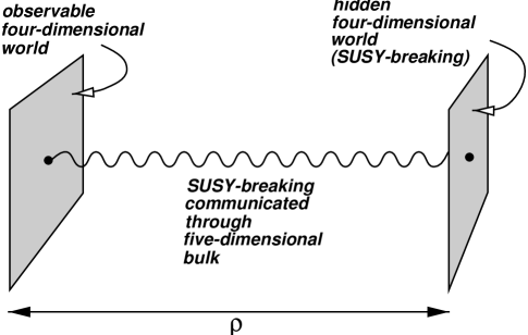
Figure 2: The Hořava-Witten scenario for communicating SUSY-breaking from a hidden world across a five-dimensional bulk of length $\rho$ to the observable world.

Question #20   Making ends meet: How can we understandQuestion #20  gauge coupling unification from stringQuestion #20    theory?

In this section we will discuss another important issue connected with strings and supersymmetry, namely gauge coupling unification. As we have seen, the strong, electroweak, and hypercharge gauge couplings appear to unify at approximately $M_{\rm MSSM}\approx 2\times 10^{16}$ GeV when extrapolated within the framework of the MSSM. Indeed, this observation is often taken as evidence for supersymmetry, which also provides elegant solutions for the finiteness and gauge hierarchy problems. Thus, the currently accepted field-theoretic scenario calls for some sort of grand unified group (GUT) above $M_{\rm MSSM}$; the MSSM gauge group and spectrum between $M_{\rm MSSM}$ and the scale of SUSY-breaking $M_{\rm SUSY}$ at which the superpartners decouple; and simply the Standard Model gauge group and spectrum below $M_{\rm SUSY}$.

This is a compelling picture, except for various problems. First, $M_{\rm MSSM}$ is close to the Planck scale, but gravity is not incorporated. Second, one would in principle like to explain the spectrum of the MSSM — e.g., to explain why there are three generations, or to derive the fermion mass matrices. Third, if there is a GUT theory above $M_{\rm MSSM}$, what about proton-lifetime problems? One requires some sort of doublet-triplet splitting mechanism, as was discussed in Question #14. Finally, why should we require gauge coupling unification at all? This is, after all, only a theoretical prejudice, and is not required for the consistency of the model.

20.1  The predictions from string theory

Of course, string theory can solve these problems. First, as we have seen, it naturally incorporates quantized gravity, in the sense that a spin-two massless particle (the graviton) always appears in the string spectrum. Second, $N=1$ supersymmetric field theories with non-abelian gauge groups naturally appear as the limits of a certain class of string models (the heterotic strings). Third, string theory can provide, in principle, a uniform framework for understanding three generations, fermion matrices, doublet-triplet splitting mechanism, etc. — in principle, there are no free parameters! Finally, it also turns out that independently of the existence of a unified gauge symmetry, heterotic string theories always give rise to a natural unification of gauge couplings. Indeed, in heterotic string theory, the gauge and gravitational couplings automatically unify [94] to form a single coupling constant $g_{\rm string}$:

$$8\pi{G_{N}\over\alpha^{\prime}}~{}=~{}g_{i}^{2}\,k_{i}~{}=~{}g_{\rm string}^{2}~{}.$$ (38)

Here $G_{N}$ is the gravitational (Newton) coupling; $\alpha^{\prime}$ is the Regge slope (which sets the mass scale for string theory); $g_{i}$ are the gauge couplings; and the normalization constants $k_{i}$ are the affine levels (also sometimes called Kač-Moody levels) at which the different group factors are realized. For non-abelian group factors we have $k_{i}\in\mathchoice{\hbox{\cmss Z\kern-3.99994ptZ}}{\hbox{\cmss Z\kern-3.99994ptZ}}{\lower 0.9pt\hbox{\cmsss Z\kern-2.79996ptZ}}{\lower 1.2pt\hbox{\cmsss Z\kern-2.79996ptZ}}^{+}$, while for $U(1)$ gauge factors the $k_{i}$ are arbitrary. Thus, string theory appears to give us precisely the features we want.

There are, however, some crucial differences between string theory and field theory. First, string theory is a finite theory: the gauge couplings run only within the framework of the string low-energy effective theory. Second, in string theory all couplings are ultimately dynamical variables, related to the expectation values of scalar moduli fields. The third difference is the dependence on the affine levels $k_{i}$. These levels are essentially normalizations, and are therefore analogous to the hypercharge normalization $k_{Y}=5/3$ which appears in $SU(5)$ or $SO(10)$ embeddings, but in string theory such normalizations also appear for the non-abelian gauge couplings as well. It turns out that the most easily constructed string models have $k_{i}=1$ for non-abelian factors.

The most important difference concerns the scale of the unification. The string unification scale is set by $\alpha^{\prime}$ (which in turn is set by Planck scale), and at the one-loop level one finds [95]:

$$M_{\rm string}~{}\approx~{}g_{\rm string}~{}\times~{}5\times 10^{17}~{}{\rm GeV}~{}.$$ (39)

Since extrapolation of low-energy data suggests that $g_{\rm string}\approx{\cal O}(1)$, we thus find that $M_{\rm string}\approx 5\times 10^{17}$ GeV — a factor of 20 discrepancy relative to the MSSM prediction!

Is this is a major problem? A factor of 20 sounds large, but this is only a 10% effect in the logarithms of the mass scales. Unfortunately, however, this discrepancy leads to wildly incorrect values for the low-energy observables $\sin^{2}\theta_{W}$ and $\alpha_{\rm strong}$ at the weak scale. In other words, if we start our MSSM running of gauge couplings down from $M_{\rm string}$ rather than from $M_{\rm MSSM}$, we find that string theory predicts values for these quantities which differ from their experimentally observed values by many standard deviations. This is the problem of gauge coupling unification in string theory. Essentially, given the high-energy predictions of string theory and our low-energy experimental couplings, we face the classic question: how can we make the two ends meet?

20.2  Overview of possible solutions

Over the past decade, a number of solutions to this question have been proposed. We shall here outline only six possible classes of solutions. The reader should consult Ref. [74] for a more complete discussion of these and other solutions.

The first solution reconciles $M_{\rm MSSM}$ and $M_{\rm string}$ by assuming that the three low-energy gauge couplings indeed unify at $M_{\rm MSSM}$ because of the presence of a unifying gauge symmetry group $G$ at that scale, whereupon the new unified gauge coupling $g_{G}$ runs upwards to $M_{\rm string}$ where it unifies with the gravitational coupling. Thus, at the string scale, we are essentially realizing the GUT group $G$ as our gauge symmetry: these are “string GUT models”. Note that in this context we therefore consider only those unification groups $G$ such as $SU(5)$ or $SO(10)$ which are simple. An essential property of such groups is that they require a Higgs scalar representation in the adjoint of $G$ in order to break $G$ down to the MSSM gauge group.

The second possible solution makes use of the affine levels $k_{i}$ that appear in the string unification relation in Eq. (38). Indeed, in string theory, these levels $k_{i}$ need not take the values $(k_{Y},k_{2},k_{3})=(5/3,1,1)$ that we naïvely expect them to have in the MSSM. It is then possible that non-standard values for these levels could alter the runnings in such a way as to reconcile the string unification scale with the MSSM unification scale. This would clearly be a stringy effect.

The third solution supposes that there can be large “heavy string threshold corrections” at the string scale. These corrections represent the contributions from the infinite towers of massive (Planck-scale) string states that are otherwise neglected in an analysis of the purely massless string spectrum. This would also be an intrinsically stringy effect.

A fourth solution involves “light SUSY thresholds” — the corrections that arise due to the breaking of supersymmetry — and are typically analyzed in field theory.

A fifth solution involves extra matter beyond the MSSM at intermediate mass scales. While introducing such matter may seem ad hoc from the field-theory perspective, it turns out that certain exotic non-MSSM states appear in, and are actually required for the self-consistency of, many realistic string models.

Finally, a sixth solution [92] involves possible effects due to non-perturbative string physics. For example, as we have seen, recent developments in string duality suggest that at strong coupling, the behavior of heterotic strings can be modelled by other theories for which the heterotic string prediction in Eq. (38) is no longer valid. This then effectively loosens the tight constraints between the gauge couplings and the gravitational coupling, which in turn enables one to separate the gauge-coupling unification scale from the gravitationally-determined string scale.

Thus, we are faced with one over-riding question: Which solution(s) to the problem — i.e., which “path to unification” — does string theory actually take?

It is perhaps worth emphasizing that this a much more difficult question in string theory than it would be in field theory. In field theory, one can imagine rather easily building a model that realizes any one of the above proposals. In string theory, however, there are deeper string consistency constraints which arise due to the fact that four-dimensional (spacetime) physics is ultimately derived from two-dimensional (worldsheet) physics. Thus four-dimensional spectra, gauge symmetries, couplings, etc., are all ultimately determined or constrained by worldsheet symmetries. This tends to make it difficult, when string model-building, to realize one given desirable phenomenological feature in one sector of a string model without upsetting some other desired feature in a different sector of the model.

The question, then, is to determine which of the above potential solutions to the string unification problem are self-consistent in string theory, and can be realized in actual realistic string models.

20.3  Current status

We shall now give a quick summary of the current status of some of these proposed solutions. A more detailed review (along with appropriate references) can be found in Ref. [74].

String GUT models:   As mentioned above, the goal in this approach is to construct realistic string GUT models — i.e., string models whose low-energy limits reproduce standard $SU(5)$ or $SO(10)$ unification scenarios. The major problem that one faces, however, is that while it is generally easy to obtain the required gauge group, obtaining the required matter representations has proven to be very difficult. The fundamental reason for this difficulty is that: (i) the string requirement that the worldsheet conformal field theory be unitary ends up restricting the allowed massless matter representations that the string model can produce; and (ii) for GUT symmetry breaking, one requires a Higgs scalar transforming in the adjoint of the GUT gauge group. Together, these two requirements imply that one must realize the GUT gauge symmetry at an affine level $k_{\rm GUT}\geq 2$, and historically it has proven to be a highly non-trivial task to construct such a higher-level string GUT model with three generations [96, 97, 98].

At present, the three-generation problem has been solved at level two only in the case of $SU(5)$ [97, 98, 99]. At level three, however, there currently exist three-generation models for $SU(5)$, $SU(6)$, $SO(10)$, and $E_{6}$ [100]. However, much phenomenological analysis of these models still remains to be done. In some cases, these models tend to have extra chiral matter, or unsuitable couplings. Doublet-triplet splitting also remains a problem, and appears to require fine-tuning. There are also rather tight constraints [101] concerning the allowed representations and couplings for these models which restrict their phenomenologies significantly. However, the important point is that the issues concerning string GUT model-building now seem to be more of a technical rather than fundamental nature, and further progress can be expected.

Non-Standard Levels and Hypercharge Normalizations:   In this solution to the unification problem, one attempts to realize the MSSM gauge group and particle content in a given model, but to reconcile the discrepancy between $M_{\rm MSSM}$ and $M_{\rm string}$ by having non-standard values for the levels $(k_{Y},k_{2},k_{3})$. A straightforward analysis [102, 103] shows that in order to do the job, the required levels would be:

$$k_{2}=k_{3}=1,2~{};~{}~{}~{}~{}~{}~{}k_{Y}/k_{2}\approx 1.45-1.5~{}.$$ (40)

Thus, restricting our attention the simpler level-one models, the question arises: can one even realize realistic string models with $k_{Y}$ in this range?

This question is motivated by the observation that the standard $SO(10)$ hypercharge embedding naturally leads to the MSSM value $k_{Y}=5/3$, and most trivial modifications or extensions to this embedding tend to increase $k_{Y}$. Thus, more generally, we ask whether it is even possible to realize hypercharge embeddings with $k_{Y}<5/3$, and whether this would cause undesirable effects on the rest of such a string model. Note that one always must have $k_{Y}\geq 1$ in any string model containing at least the MSSM spectrum [104].

The current status of this approach is as follows. In general, it is very difficult to arrange to have $k_{Y}<5/3$ in string theory [103, 98]. However, some self-consistent string models with $k_{Y}<5/3$ have been constructed [98]. Unfortunately, all of these models have unwanted fractionally charged states that could survive in their light spectra. This is to be expected, since there is a general result [104] that if a string model is to completely avoid fractionally-charged color-neutral string states, then its affine levels must obey the relation

$$3\,k_{Y}+3\,k_{2}+4\,k_{3}~{}=~{}0~{}~{}~{}({\rm mod}~{}12)~{}.$$ (41)

For $k_{2}=k_{3}=1,2$, this implies $k_{Y}/k_{2}\geq 5/3$. Of course, it is possible that fractionally charged states appear but are extremely massive, or that they might bind together into color-neutral objects under the influence of extra hidden-sector interactions. A general classification of the binding scenarios that can eliminate such fractionally charged states has been performed [103], but no string model has yet been constructed which realizes these scenarios.

Heavy string threshold corrections:   Heavy string threshold corrections are the contributions due to the infinite towers of massive Planck-scale string states that are otherwise neglected when deriving a low-energy effective action from the string. In order to reconcile the values of the three low-energy gauge couplings $g_{i}$ with string-scale unification, it turns out that such corrections $\Delta_{i}$ must have the relative sizes

$$\Delta_{\hat{Y}}-\Delta_{2}\approx-28~{},~{}~{}~{}\Delta_{\hat{Y}}-\Delta_{3}\approx-58~{},~{}~{}~{}\Delta_{2}-\Delta_{3}\approx-30~{}.$$ (42)

where $\hat{Y}\equiv Y/\sqrt{5/3}$ is the renormalized hypercharge. These corrections are quite sizable, and the fundamental question is then how to obtain corrections of this size.

The formalism for calculating these corrections was first derived in Ref. [95] and more recently refined in Ref. [105]. From these results, a number of theoretical mechanisms were identified for making these corrections sufficiently large. Perhaps the most obvious mechanism [106] is to construct a string model with a large modulus (such as a large compactified dimension), for as the size of such a radius is increased, various momentum states become lighter and lighter. The contributions of such states to the threshold corrections therefore become more substantial, ultimately leading to a decompactification of the theory. Unfortunately, it is not known why a given string model should be expected to have such a large modulus. Indeed, the general expectation is that in realistic string models, moduli should settle at or near the self-dual point for which moduli are of order one [107].

Explicit calculations of these threshold corrections have been carried out within several realistic string models. Here the term “realistic” denotes string models with the following properties: $N=1$ spacetime SUSY; appropriate gauge groups [such as $SU(3)\times SU(2)\times U(1)$, Pati-Salam $SO(6)\times SO(4)$, or flipped $SU(5)\times U(1)$]; the proper massless observable spectrum (including three complete chiral MSSM generations with correct quantum numbers, hypercharges, and Higgs scalar representations); and anomaly cancellation. Many realistic models also exhibit additional attractive features, such as a semi-stable proton, proper fermion mass hierarchy, and a heavy top quark. A collection of such models, all of which are realized in the free-fermionic construction with an underlying $\mathchoice{\hbox{\cmss Z\kern-3.99994ptZ}}{\hbox{\cmss Z\kern-3.99994ptZ}}{\lower 0.9pt\hbox{\cmsss Z\kern-2.79996ptZ}}{\lower 1.2pt\hbox{\cmsss Z\kern-2.79996ptZ}}_{2}\times\mathchoice{\hbox{\cmss Z\kern-3.99994ptZ}}{\hbox{\cmss Z\kern-3.99994ptZ}}{\lower 0.9pt\hbox{\cmsss Z\kern-2.79996ptZ}}{\lower 1.2pt\hbox{\cmsss Z\kern-2.79996ptZ}}_{2}$ orbifold structure, can be found in Ref. [108].

Unfortunately, the results found within these models are not encouraging: in each of the realistic string models of Ref. [108], it is found [109] that threshold corrections are unexpectedly small, and moreover they have the wrong sign. For example, in one such string model it was found that

$$\Delta_{\hat{Y}}-\Delta_{2}~{}\approx~{}1.6~{},~{}~{}~{}~{}\Delta_{\hat{Y}}-\Delta_{3}~{}\approx~{}5~{}$$ (43)

which does not fare well against Eq. (42). This behavior seems to be generic to the entire class of realistic string models in Ref. [108]. Thus it seems that threshold corrections by themselves are not able to resolve the discrepancy with the low-energy couplings in these realistic string models. Indeed, despite some interesting proposals [110], there do not presently exist any realistic string models with small moduli for which the threshold corrections are sufficiently large.

Light SUSY thresholds and intermediate-scale gauge structure:   Light SUSY thresholds are the effects that arise from SUSY-breaking at some intermediate scale: they can be parametrized in terms of the usual soft SUSY-breaking parameters $\{m_{0},m_{1/2},m_{h},m_{\tilde{h}}\}$, or one can take non-universal boundary terms for the sparticle masses. Similarly, the effects from intermediate-scale gauge structure arise whenever there is a gauge symmetry, such as $SO(6)\times SO(4)$ or flipped $SU(5)\times U(1)$, which is broken at some intermediate scale $M_{I}$. Such effects are then parametrized in terms of $M_{I}$. Both of these effects are analyzed purely in terms of the low-energy field theory derived from the string, and consequently their evaluation proceeds exactly as in field theory. A detailed calculation of these effects must also include two-loop corrections, the effects of Yukawa couplings, and even the effects of scheme conversion (from the $\overline{\rm DR}$ scheme in which the string scale is evaluated to the $\overline{\rm MS}$ scheme through which the low-energy couplings are extracted from experiment). Within the context of the low-energy effective theories derived from the realistic string models in Ref. [108], such a calculation has been performed [109]. The results indicate that the light SUSY thresholds are generally insufficient to resolve the discrepancies, and that the effects of intermediate gauge structure in the realistic string models only enlarge the disagreement with experiment! This latter result is surprising, given that $M_{I}$ can be tuned in principle to any value below $M_{\rm string}$, and serves to illustrate the rather tight (and predictive) constraints that a given string model provides.

Extra Matter Beyond the MSSM:   Finally, there is the possibility of extra matter beyond the MSSM. While all of the above results assumed only the MSSM spectrum, string theory often requires that additional exotic states appear in the massless spectrum. Their effects must therefore be included. Such states appear in a majority of the realistic string models, usually appear in vector-like representations, and ultimately have masses determined by cubic and higher-order terms in the superpotential (which are determined in turn by the specific SUSY-breaking mechanism employed, as well as by a host of additional factors). In one string model, for example, it has been estimated [111] that such extra states will naturally sit at an intermediate scale $\approx 10^{11}$ GeV. In the realistic string models [108] with $SU(3)\times SU(2)\times U(1)$ gauge groups, such matter typically arises in rather specific $SU(3)\times SU(2)\times U(1)_{Y}$ representations such as $({\bf 3},{\bf 2})_{1/6}$, $(\overline{{\bf 3}},{\bf 1})_{1/3}$, $(\overline{{\bf 3}},{\bf 1})_{1/6}$, and $({\bf 1},{\bf 2})_{0}$. While the first two representations can be fit into standard $SO(10)$ mutliplets, the remaining two cannot, and are truly exotic.

What is remarkable, however, is that this extra matter is just what is needed: because of their unusual hypercharge assignments, these representations have one-loop beta-function coefficients $b_{i}$ where $b_{1}$ turns out to be much smaller than $b_{2}$ or $b_{3}$. These representations therefore have the potential to modify the running of the $SU(2)$ and $SU(3)$ couplings without seriously affecting the $U(1)$ coupling. Moreover, in some string models, these extra non-MSSM matter representations also appear in precisely the right combinations to do the job. Details can be found in Ref. [109]. Similar scenarios using such extra non-MSSM matter can also be found, e.g., in Ref. [112]. Thus, on the basis of this evidence, it appears that extra intermediate-scale matter beyond the MSSM may turn out to be the string-preferred route to string-scale unification. It is remarkable that string theory, which predicts an unexpectedly high unification scale, often also simultaneously predicts precisely the extra exotic matter necessary to reconcile this higher scale with the observed low-energy couplings.

  

Postscript

In this article, we have surveyed a number of questions and issues that arise in supersymmetric particle physics, ranging from the MSSM at the lowest scales to string theory at the highest scales. It is remarkable that supersymmetry not only provides a window into physics at so many different energy regimes, but also has such a profound impact in all of these areas. Indeed, at the very least it either refines old questions or proposes new ones, and in most cases it actually changes the language of the debate. Supersymmetry is perhaps the only extension of the Standard Model which has such a direct impact on so many types of new phenomena, including gravity. Moreover, as we have seen, supersymmetry has global applications, ranging from high-energy accelerator experiments to astrophysics and cosmology. The questions that supersymmetry prompts therefore provide unique opportunities for studying all sorts of new physics, and finding the answers to any of these questions — from the most phenomenological to the most theoretical — will undoubtedly teach us much about the physics that we expect to be exploring in the twenty-first century.

  

Acknowledgments

We would like to thank J. Bagger, A. Kusenko, P. Langacker, J. March-Russell, and N. Polonsky for many helpful discussions, and especially K.S. Babu, T. Gherghetta, G. Kane, and M. Peskin for their comments on this article. This work was supported in part by DOE Grant No. DE-FG02-90ER40542. CK would also like to acknowledge the generous support of Helen and Martin Chooljian, and the hospitality of the Aspen Center for Physics where parts of this work were completed.

References

- [1] J. Wess and J. Bagger, Introduction to Supersymmetry, 2nd Ed. (Princeton University Press, 1992); H.P. Nilles, Phys. Rep. 110 (1984) 1; H. Haber and G. Kane, Phys. Rep. 117 (1985) 75.
- [2] S. Dimopoulos and D. Sutter, Nucl. Phys. B452 (1995) 496.
- [3] S. Ferrara, L. Girardello, and F. Palumbo, Phys. Rev. D20 (1979) 403; S. Dimopoulos and H. Georgi, Nucl. Phys. B193 (1981) 150.
- [4] S. Weinberg, Phys. Rev. D26 (1982) 287.
- [5] G. Farrar and P. Fayet, Phys. Lett. B76 (1978) 575; S. Dimopoulos, S. Raby, and F. Wilczek, Phys. Lett. B112 (1982) 133.
- [6] T. Banks and L. Dixon, Nucl. Phys. B307 (1988) 93; M. Kamionkowski and J. March-Russell, Phys. Rev. Lett. 69 (1992) 1485; R. Holman et al., Phys. Rev. Lett. 69 (1992) 1489.
- [7] S. Martin, Phys. Rev. D46 (1992) 2769.
- [8] L. Ibáñez and G. Ross, Nucl. Phys. B368 (1991) 3.
- [9] L. Hall, V. Kostelecky, and S. Raby, Nucl. Phys. B267 (1986) 415; H. Georgi, Phys. Lett. B169 (1986) 231.
- [10] J. Donoghue, H.P. Nilles, and D. Wyler, Phys. Lett. B128 (1983) 55.
- [11] F. Gabbiani and A. Masiero, Nucl. Phys. B322 (1989) 235; M. Dine, A. Kagan, and S. Samuel, Phys. Lett. B243 (1990) 250; F. Gabbiani, E. Gabrielli, A. Masiero, and L. Silvestrini, Nucl. Phys. B477 (1996) 321.
- [12] Y. Nir and N. Seiberg, Phys. Lett. B309 (1993) 337.
- [13] K.S Babu and S. Barr, Phys. Lett. B387 (1996) 87.
- [14] L. Ibáñez and G. Ross, Phys. Lett. B332 (1994) 100; P. Binétruy and P. Ramond, Phys. Lett. B350 (1995) 49; P. Binétruy, S. Lavignac, and P. Ramond, Nucl. Phys. B477 (1996) 353; R. Zhang, Phys. Lett. B402 (1997) 101; A. Nelson and D. Wright, Phys. Rev. D56 (1997) 1598.
- [15] A. Cohen, D. Kaplan, and A. Nelson, Phys. Lett. B388 (1996) 588.
- [16] N. Arkani-Hamed and H. Murayama, hep-ph/9703259.
- [17] For a nice review, see: Y. Grossman, Y. Nir, and R. Rattazzi, hep-ph/9701231.
- [18] W. Fischler, S. Paban, and S. Thomas, Phys. Lett. B289 (1992) 373.
- [19] P. Binétruy and E. Dudas, Phys. Lett. B389 (1996) 503; G. Dvali and A. Pomarol, Phys. Rev. Lett. 77 (1996) 3728.
- [20] K.S. Babu, C. Kolda, and F. Wilczek, Phys. Rev. Lett. 77 (1996) 3070; M. Dine, Y. Nir, and Y. Shirman, Phys. Rev. D55 (1997) 1501; J. Bagger et al., Phys. Rev. D55 (1997) 3188; R. Rattazzi and U. Sarid, hep-ph/9612464; F. Borzumati, hep-ph/9702307.
- [21] M. Carena et al., hep-ph/9702409.
- [22] G. Guidice and A. Masiero, Phys. Lett. B206 (1988) 480.
- [23] J. Casas, A. Lleyda and C. Muñoz, Nucl. Phys. B471 (1996) 3.
- [24] J. Gunion, H. Haber, and M. Sher, Nucl. Phys. B306 (1988) 1.
- [25] T. Gherghetta, C. Kolda, and S. Martin, Nucl. Phys. B468 (1996) 37.
- [26] A. Kusenko, P. Langacker, and G. Segrè, Phys. Rev. D54 (1996) 5824.
- [27] E. Witten, Nucl. Phys. B188 (1981) 513.
- [28] R. Roberts and G. Ross, Nucl. Phys. B377 (1992) 571; S. Kelley et al., Nucl. Phys. B398 (1993) 3; M. Drees and M. Nojiri, Phys. Rev. D47 (1993) 376; G. Kane, L. Roszkowski, C. Kolda, and J. Wells, Phys. Rev. D49 (1994) 6173; M. Carena, M. Olechowski, S. Pokorski, and C. Wagner, Nucl. Phys. B419 (1994) 213.
- [29] Recent work was inspired by the papers of M. Dine and A. Nelson, Phys. Rev. D48 (1993) 1277; M. Dine, A. Nelson, and Y. Shirman, Phys. Rev. D51 (1995) 1362; M. Dine, A. Nelson, Y. Nir, and Y. Shirman, Phys. Rev. D53 (1996) 2658.
- [30] For recent work, see: S. Abel, S. Sarkar, and P. White, Nucl. Phys. B454 (1995) 663.
- [31] U. Ellwanger, Phys. Lett. B133 (1983) 187; J. Bagger and E. Poppitz, Phys. Rev. Lett. 71 (1993) 2380; J. Bagger, E. Poppitz, and L. Randall, Nucl. Phys. B455 (1995) 59.
- [32] H.P. Nilles and N. Polonsky, hep-ph/9707249.
- [33] C. Kolda, S. Pokorski, and N. Polonsky, in preparation.
- [34] M. Cvetič and P. Langacker, Phys. Rev. D54 (1996) 3570; M. Cvetič et al., hep-ph/9703317; hep-ph/9705391.
- [35] K.R. Dienes, C. Kolda, and J. March-Russell, Nucl. Phys. B492 (1997) 104.
- [36] T. Falk, K. Olive, and M. Srednicki, Phys. Lett. B339 (1994) 248.
- [37] G. Kane and J. Wells, Phys. Rev. Lett. 76 (1996) 4458.
- [38] For a review, see: G. Jungman, M. Kamionkowski, and K. Griest, Phys. Rep. 267 (1996) 195.
- [39] P. Fayet, Phys. Rep. 105 (1984) 21.
- [40] H. Pagels and J. Primack, Phys. Rev. Lett. 48 (1982) 223.
- [41] T. Gherghetta, Nucl. Phys. B485 (1997) 25.
- [42] M. Luty and E. Ponton, hep-ph/9706268.
- [43] T. Moroi, H. Murayama, and M. Yamaguchi, Phys. Lett. B303 (1993) 289.
- [44] M. Dine, W. Fischler, and D. Nemeschansky, Phys. Lett. B136 (1984) 169.
- [45] D. Lyth and E. Stewart, Phys. Rev. D53 (1996) 1784.
- [46] I. Affleck and M. Dine, Nucl. Phys. B249 (1985) 361. M. Dine, L. Randall, and S. Thomas, Nucl. Phys. B458 (1996) 291.
- [47] L. Kofman, A. Linde, and A. Starobinskii, Phys. Rev. Lett. 73 (1994) 3195; Y. Shtanov, J. Traschen, and R. Brandenberger, Phys. Rev. D51 (1995) 5438.
- [48] R. Brustein and P. Steinhardt, Phys. Lett. B302 (1993) 196.
- [49] J.C. Pati and A. Salam, Phys. Rev. D8 (1973) 1240; H. Georgi and S.L. Glashow, Phys. Rev. Lett. 32 (1974) 438.
- [50] S. Dimopoulos, S. Raby, and F. Wilczek, Phys. Rev. D24 (1981) 1681; S. Dimopoulos and H. Georgi, Nucl. Phys. B193 (1981) 150; N. Sakai, Zeit. Phys. C11 (1981) 153; L.E. Ibáñez and G.G. Ross, Phys. Lett. B105 (1981) 439.
- [51] H. Georgi, H.R. Quinn, and S. Weinberg, Phys. Rev. Lett. 33 (1974) 451.
- [52] M.B. Einhorn and D.R.T. Jones, Nucl. Phys. B196 (1982) 475; W.J. Marciano and G. Senjanovic, Phys. Rev. D25 (1982) 3092.
- [53] For recent precision calculations, see, e.g.: U. Amaldi, W. de Boer, and H. Fürstenau, Phys. Lett. B260 (1991) 447; J. Ellis, S. Kelley, and D.V. Nanopoulos, Phys. Lett. B260 (1991) 131; P. Langacker and M. Luo, Phys. Rev. D44 (1991) 817; P. Langacker and N. Polonsky, Phys. Rev. D47 (1993) 4028; M. Carena, S. Pokorski, and C.E.M. Wagner, Nucl. Phys. B406 (1993) 59; J. Bagger, K. Matchev, and D. Pierce, Phys. Lett. B348 (1995) 443.
- [54] N. Sakai and T. Yanagida, Nucl. Phys. B197 (1982) 533; S. Weinberg, Phys. Rev. D26 (1982) 287.
- [55] E. Witten, Phys. Lett. B105 (1981) 267; D.V. Nanopoulos and K. Tamvakis, Phys. Lett. B113 (1982) 151; S. Dimopoulos and H. Georgi, Phys. Lett. B117 (1982) 287; L. Ibáñez and G. Ross, Phys. Lett. B110 (1982) 215.
- [56] A. Buras et al., Nucl. Phys. B135 (1985) 66; H. Georgi, Phys. Lett. B108 (1982) 283; A. Masiero et al., Phys. Lett. B115 (1982) 380; B. Grinstein, Nucl. Phys. B206 (1982) 387.
- [57] K. Inoue, A. Kakuto, and T. Takano, Prog. Theor. Phys. 75 (1984) 664; A. Anselm and A. Johansen, Phys. Lett. B200 (1988) 331; Z. Berezhiani and G. Dvali, Sov. Phys. Lebedeev Inst. Reps. 5 (1989) 55; R. Barbieri, G. Dvali, and M. Moretti, Phys. Lett. B312 (1993) 137.
- [58] S. Dimopoulos and F. Wilczek, ITP preprint NSF-ITP-82-07 (1982), unpublished. For a recent discussion, see: K.S. Babu and S.M. Barr, Phys. Rev. D48 (1993) 5354; Phys. Rev. D50 (1994) 3529.
- [59] D. Lee and R.N. Mohapatra, Phys. Rev. D51 (1995) 1353; L.J. Hall and S. Raby, Phys. Rev. D51 (1995) 6524.
- [60] J. Hisano, H. Murayama, and T. Yanagida, Phys. Rev. D49 (1994) 4966; K.S. Babu and S.M. Barr, Phys. Rev. D51 (1995) 2463; G. Dvali and S. Pokorski, Phys. Lett. B379 (1996) 126; S.M. Barr and S. Raby, hep-ph/9705366.
- [61] A.J. Buras, J. Ellis, M.K. Gaillard, and D.V. Nanopoulos, Nucl. Phys. B135 (1978) 66.
- [62] S. Raby, hep-ph/9501349; Z. Berezhiani, hep-ph/9602325.
- [63] H. Georgi and C. Jarlskog, Phys. Lett. B86 (1979) 297.
- [64] M. Gell-Mann, P. Ramond, and R. Slansky, in Supergravity (edited by P. van Nieuwenhuizen and D.Z. Freedman), North-Holland, Amsterdam (1979); T. Yanagida, in Proceedings of the Workshop on Unified Theories and Baryon Number in the Universe (edited by A. Sawada and A. Sugamoto), K.E.K. preprint 79-18 (1979); R.N. Mohapatra and G. Senjanovic, Phys. Rev. Lett. 44 (1980) 912.
- [65] H. Arason et al., Phys. Rev. D47 (1993) 232; G. Anderson et al., Phys. Rev. D49 (1994) 3660.
- [66] X.G. He and S. Meljanac, Phys. Rev. D41 (1990) 1620; S. Dimopoulos, L.J. Hall, and S. Raby, Phys. Rev. Lett. 68 (1992) 1984; Phys. Rev. D45 (1992) 4192; G. Anderson et al., Phys. Rev. D47 (1993) 3702.
- [67] K.S. Babu and R.N. Mohapatra, Phys. Rev. Lett. 70 (1993) 2845; Phys. Rev. Lett. 74 (1995) 2418; K.S. Babu and S.M. Barr, hep-ph/9512389; Phys. Rev. Lett. 75 (1995) 2088.
- [68] J. Ellis, J. Lopez, and D.V. Nanopoulos, Phys. Lett. B245 (1990) 375.
- [69] N. Seiberg, hep-th/9506077; K. Intriligator and N. Seiberg, Nucl. Phys. Proc. Suppl. 55B (1997) 157.
- [70] C. Montonen and D. Olive, Phys. Lett. B72 (1977) 117.
- [71] For introductions and reviews, see: M.B. Green, J.H. Schwarz, and E. Witten, Superstring Theory, Vols. 1 & 2 (Cambridge University Press, Cambridge, 1987); M. Dine, ed., String Theory in Four Dimensions (North-Holland, Amsterdam, 1988); B. Schellekens, ed., Superstring Construction (North-Holland, Amsterdam, 1989); J. Polchinski, What is String Theory?, 1994 Les Houches Summer School Lectures, hep-th/9411028.
- [72] For recent general discussions on various aspects of string phenomenology and string model-building, see, e.g.: L.E. Ibáñez, hep-th/9112050; hep-th/9505098; I. Antoniadis, hep-th/9307002; M. Dine, hep-ph/9309319; J.L. Lopez, Surveys H.E. Phys. 8 (1995) 135; J.L. Lopez and D.V. Nanopoulos, hep-ph/9511266; J.D. Lykken, hep-ph/9511456; hep-th/9607144; F. Quevedo, hep-th/9603074; hep-ph/9707434; A.E. Faraggi, hep-ph/9707311; G. Cleaver, hep-th/9708023; Z. Kakushadze, G. Shiu, S.-H.H. Tye, and Y. Vtorov-Karevsky, hep-th/9710149; and references therein.
- [73] T.R. Taylor, hep-ph/9510281; F. Quevedo, hep-th/9511131.
- [74] K.R. Dienes, Phys. Reports 287 (1997) 447 [hep-th/9602045].
- [75] J. Polchinski, Prog. Theor. Phys. Suppl. 123 (1996) 9; Rev. Mod. Phys. 68 (1996) 1245; hep-th/9611050; J. Schwarz, hep-th/9607201; M. Duff, Int. J. Mod. Phys. A11 (1996) 5623; M. Dine, hep-th/9609051; A. Sen, hep-th/9609176; M.R. Douglas, hep-th/9610041; P.K. Townsend, hep-th/9612121; S. Förste and J. Louis, hep-th/9612192; S. Kachru, hep-th/9705173.
- [76] P. Ramond, Phys. Rev. D3 (1971) 2415.
- [77] L.J. Dixon and J.A. Harvey, Nucl. Phys. B274 (1986) 93; A Sen, Nucl. Phys. B278 (1986) 289; T. Banks, L. Dixon, D. Friedan, and E. Martinec, Nucl. Phys. B299 (1988) 613.
- [78] J.D. Blum and K.R. Dienes, Phys. Lett. B414 (1997) 260; hep-th/9707160 (to appear in Nucl. Phys. B).
- [79] M.B. Green and J. Schwarz, Phys. Lett. B149 (1984) 117.
- [80] M. Dine, N. Seiberg, and E. Witten, Nucl. Phys. B289 (1987) 589.
- [81] See, e.g.: G. Moore, Nucl. Phys. B293 (1987) 139; Erratum: ibid. B299 (1988) 847; T.R. Taylor, Nucl. Phys. B303 (1988) 543; J. Balog and M.P. Tuite, Nucl. Phys. B319 (1989) 387; K.R. Dienes, Phys. Rev. D42 (1990) 2004, Phys. Rev. Lett. 65 (1990) 1979; T. Gannon and C.S. Lam, Phys. Rev. D46 (1992) 1710.
- [82] J. Scherk and J.H. Schwarz, Phys. Lett. B82 (1979) 60.
- [83] R. Rohm, Nucl. Phys. B237 (1984) 553.
- [84] K.R. Dienes, Nucl. Phys. B429 (1994) 533; hep-th/9409114; hep-th/9505194.
- [85] K.R. Dienes, M. Moshe, and R.C. Myers, Phys. Rev. Lett. 74 (1995) 4767; hep-th/9506001.
- [86] I. Antoniadis, Phys. Lett. B246 (1990) 377; I. Antoniadis, C. Muñoz, and M. Quirós, Nucl. Phys. B397 (1993) 515; I. Antoniadis and K. Benakli, Phys. Lett. B326 (1994) 69.
- [87] S. Ferrara, C. Kounnas, and M. Porrati, Phys. Lett. B197 (1987) 135; Phys. Lett. B206 (1988) 25; Nucl. Phys. B304 (1988) 500; S. Ferrara, C. Kounnas, M. Porrati, and F. Zwirner, Nucl. Phys. B318 (1989) 75.
- [88] C. Bachas, hep-th/9503030; J.G. Russo and A.A. Tseytlin, Nucl. Phys. B461 (1996) 131; A.A. Tseytlin, hep-th/9510041; M. Spalinski and H.P. Nilles, Phys. Lett. B392 (1997) 67; I. Shah and S. Thomas, hep-th/9705182.
- [89] I. Antoniadis, C. Bachas, D.C. Lewellen, and T. Tomaras, Phys. Lett. B207 (1988) 441.
- [90] See, e.g., H.P. Nilles, Phys. Lett. B115 (1982) 193; Nucl. Phys. B217 (1983) 366; Int. J. Mod. Phys. AA5 (1990) 4199; J.P. Derendinger, L.E. Ibáñez, and H.P. Nilles, Phys. Lett. B155 (1985) 65; M. Dine, R. Rohm, N. Seiberg, and E. Witten, Phys. Lett. B156 (1985) 55; T.R. Taylor, Phys. Lett. B164 (1985) 43; Phys. Lett. B252 (1990) 59; C. Kounnas and M. Porrati, Phys. Lett. B191 (1987) 91; P. Binétruy and M.K. Gaillard, Phys. Lett. B232 (1989) 83; Phys. Lett. B253 (1991) 119; Nucl. Phys. B358 (1991) 121; A. Font, L.E. Ibáñez, D. Lüst, and F. Quevedo, Phys. Lett. B249 (1990) 35; J.A. Casas, Z. Lalak, C. Muñoz, and G.G. Ross, Nucl. Phys. B347 (1990) 243; V.S. Kaplunovsky and J. Louis, Phys. Lett. B306 (1993) 269; Nucl. Phys. B422 (1994) 57; P. Binétruy, M.K. Gaillard, and Y.Y. Wu, Nucl. Phys. B493 (1997) 27; and references therein.
- [91] P. Hořava and E. Witten, Nucl. Phys. B460 (1996) 506.
- [92] E. Witten, Nucl. Phys. B471 (1996) 135; P. Hořava and E. Witten, Nucl. Phys. B475 (1996) 94.
- [93] P. Hořava, Phys. Rev. D54 (1996) 7561; T. Banks and M. Dine, Nucl. Phys. B479 (1996) 173; hep-th/9609046; E. Caceres, V.S. Kaplunovsky, and I.M. Mandelberg, hep-th/9606036; T.J. Li, J.L. Lopez, and D.V. Nanopoulos, hep-ph/9702237; hep-ph/9704247; E. Dudas and C. Grojean, hep-th/9704177; I. Antoniadis and M. Quirós, hep-th/9705037; hep-th/9707208; H.P. Nilles, M. Olechowski, and M. Yamaguchi, hep-th/9707143; Z. Lalak and S. Thomas, hep-th/9707223. E. Dudas, hep-th/9709043; K. Choi, H.B. Kim, and C. Muñoz, hep-th/9711158; A. Lukas, B.A. Ovrut, and D. Waldram, hep-th/9711197.
- [94] P. Ginsparg, Phys. Lett. B197 (1987) 139.
- [95] V.S. Kaplunovsky, Nucl. Phys. B307 (1988) 145; Erratum: ibid. B382 (1992) 436.
- [96] D.C. Lewellen, Nucl. Phys. B337 (1990) 61; A. Font, L.E. Ibáñez, and F. Quevedo, Nucl. Phys. B345 (1990) 389; G. Aldazabal, A. Font, L.E. Ibáñez, and A.M. Uranga, Nucl. Phys. B452 (1995) 3; S. Chaudhuri, S.-W. Chung, G. Hockney, and J.D. Lykken, Nucl. Phys. B456 (1995) 89; A.A. Maslikov, I. Naumov, and G.G. Volkov, Int. J. Mod. Phys. A11 (1996) 1117; J. Erler, hep-th/9602032; G. Cleaver, hep-th/9604183.
- [97] G. Aldazabal, A. Font, L.E. Ibáñez, and A.M. Uranga, Nucl. Phys. B465 (1996) 34.
- [98] S. Chaudhuri, G. Hockney, and J.D. Lykken, Nucl. Phys. B469 (1996) 357.
- [99] D. Finnell, Phys. Rev. D53 (1996) 5781.
- [100] Z. Kakushadze and S.-H.H. Tye, Phys. Rev. Lett. 77 (1996) 2612; Phys. Lett. B392 (1997) 335; Phys. Rev. D55 (1997) 7878; Phys. Rev. D55 (1997) 7896; hep-ph/9705202.
- [101] K.R. Dienes and J. March-Russell, Nucl. Phys. B479 (1996) 113; K.R. Dienes, Nucl. Phys. B488 (1997) 141.
- [102] J.A. Casas and C. Muñoz, Phys. Lett. B214 (1988) 543; L. Ibáñez, Phys. Lett. B318 (1993) 73; K. Benakli and G. Senjanovic, Phys. Rev. D54 (1996) 5734.
- [103] K.R. Dienes, A.E. Faraggi, and J. March-Russell, Nucl. Phys. B467 (1996) 44.
- [104] A.N. Schellekens, Phys. Lett. B237 (1990) 363.
- [105] E. Kiritsis and C. Kounnas, Nucl. Phys. Proc. Suppl. 41 (1995) 331; Nucl. Phys. B442 (1995) 472; hep-th/9507051; Nucl. Phys. Proc. Suppl. 45 (1996) 207; E. Kiritsis, C. Kounnas, P.M. Petropoulos, and J. Rizos, Phys. Lett. B385 (1996) 87.
- [106] L.J. Dixon, V.S. Kaplunovsky, and J. Louis, Nucl. Phys. B355 (1991) 649.
- [107] A. Font, L.E. Ibáñez, D. Lüst, and F. Quevedo, Phys. Lett. B245 (1990) 401; M. Cvetič, A. Font, L.E. Ibáñez, D. Lüst, and F. Quevedo, Nucl. Phys. B361 (1991) 194; B. de Carlos, J.A. Casas, and C. Muñoz, Nucl. Phys. B399 (1993) 623.
- [108] I. Antoniadis, J. Ellis, J. Hagelin, and D.V. Nanopoulos, Phys. Lett. B231 (1989) 65; A.E. Faraggi, D.V. Nanopoulos, and K. Yuan, Nucl. Phys. B335 (1990) 347; J.L. Lopez, D.V. Nanopoulos, and K. Yuan, Nucl. Phys. B399 (1993) 654; I. Antoniadis, G.K. Leontaris, and J. Rizos, Phys. Lett. B245 (1990) 161; A.E. Faraggi, Phys. Lett. B278 (1992) 131; Nucl. Phys. B387 (1992) 239; Phys. Lett. B302 (1993) 202.
- [109] K.R. Dienes and A.E. Faraggi, Phys. Rev. Lett. 75 (1995) 2646; Nucl. Phys. B457 (1995) 409.
- [110] P. Mayr, H.P. Nilles, and S. Stieberger, Phys. Lett. B317 (1993) 53; H.P. Nilles and S. Stieberger, Phys. Lett. B367 (1996) 126; Nucl. Phys. B499 (1997) 3.
- [111] A.E. Faraggi, Phys. Rev. D46 (1992) 3204.
- [112] I. Antoniadis, J. Ellis, S. Kelley, and D.V. Nanopoulos, Phys. Lett. B272 (1991) 31; S. Kelley, J.L. Lopez, and D.V. Nanopoulos, Phys. Lett. B278 (1992) 140; D. Bailin and A. Love, Phys. Lett. B280 (1992) 26; M.K. Gaillard and R. Xiu, Phys. Lett. B296 (1992) 71; S.P. Martin and P. Ramond, Phys. Rev. D51 (1995) 6515; B.C. Allanach and S.F. King, hep-ph/9601391; C. Bachas, C. Fabre, and T. Yanagida, Phys. Lett. B370 (1996) 49; J.L. Lopez and D.V. Nanopoulos, Phys. Rev. Lett. 76 (1996) 1566.