Abstract

The soft gluon part of a proton wave function is investigated and compared with an onium case. It is argued that at every step of the gloun cascade new color structures appear. Dipole equation kernel emerges when a diquark limit is assumed.

1 Introduction

A soft gluon evolution in QCD is governed by a so called BFKL equation which has been originally derived in [1, 2, 3]. In a series of papers [4] by Nikolaev and Zaharkov and independently [5, 6, 7] by Mueller and collaborators a dipole picture of the gluon cascade has been developed and shown to be equivalent to the BFKL evolution. For its simplicity and probabilistic interpretation the QCD dipole picture has been successfully applied to describe proton structure function at low $x$ measured at HERA [8, 9], to proton-nucleon scattering [10] to photon-photon scattering [11] and Pomeron phenomenology [12, 13].

The most convenient way to introduce the dipole picture is to consider an $onium$: a $q\bar{q}$ state of two heavy fermions. The $onium$ wave function consists of the original fermions and many gluons emitted during the time evolution. In order to calculate the $n$ gluon component of the wave function one employs:

1. a light-cone perturbation theory and leading logarithmic approximation for the longitudinal phase-space integrations;

2. a large $N_{\rm c}$ expansion in which every gluon line in color space can be represented as a $q\bar{q}$ pair.

In the first step (1 gluon component of the wave function) a quark component of the gluon and the heavy antiquark from the original $onium$ which form a color singlet are said to constitute a dipole. A second dipole is formed from an antiquark component of the gluon and the heavy quark from the $onium$. The key observation leading to the formulation of the dipole picture is that in the next steps (2 and more gluon component of the wave function) each dipole emits subsequent gluons independently of other dipoles; in other words there is no interference between the different dipoles. This leads to a factorization of a kernel describing gluon emission from a dipole.

In this way real gluon emissions are taken into account. Total probability of real emissions is UV divergent but IR finite. Virtual corrections, which have to be included as well, make this probability finite and the complete kernel is identical to the one of BFKL.

In [8, 9] it was assumed that $q\bar{q}$ (dipole) configuration can be found in a proton and this dipole configuration gives the dominant contribution to the soft gluon density in a proton. This assumption leads to the same soft gluon density in the case of a proton as in the case of an onium (up to the normalization factor). Thus it becomes tempting to get this result by explicit calculation. Indeed, one can naively expect that a 3 (or rather $N_{\rm c}$) quark configuration in a color singlet state surrounds itself by dipoles during the evolution of the gluon cascade in close resemblance to the onium case.

In this letter we show that this naive picture breaks down. The reason is quite simple: there are interference diagrams between dipoles and a proton which cannot be neglected as it was in the case of the onium. There the interference diagrams between different dipoles could have been discarded since they were non-leading in $N_{\rm c}$. However, in the case of a proton a number of quarks is $N_{\rm c}$ and this factor enhances the non-leading interference contributions. As a result there is no universal emission kernel which factorizes in subsequent gluon emissions and moreover the complicated color structures emerge. Whether a simple probabilistic picture can be recovered by introducing higher color multipoles remains still an open question.

It is however instructive to investigate a diquark limit, $i.e.$ a limit in which 2 (or $N_{\rm c}-1$) quarks are localized in one point. In that case the original proton reduces to a quark-diquark system which is in fact identical to an onium state. We have checked by explicit calculation that this diquark configuration of valence quarks in a proton leads to the soft gluon density of a dipole type.

In Section 2, we calculate the wave function of a proton in analogy with [5]. Then the square of a proton wave function is compared with the onium case. In Section 3, we show that in the limit where two valence quarks are localized in the same transverse position (diquark approximation) the dipole equation emerges. In Section 4 we shortly summarize our findings.

2 Wave function of a proton

In analogy with Refs.[5, 7] we decompose the proton state $|\Psi>$ in the basis of the eigenstates of the QCD evolution hamiltonian $H_{0}$. The $3+n$ particle (three quarks and $n$ soft gluons) component of $|\Psi>$ is defined as:

$${\psi^{(n)}}^{~{}ijk~{}{a_{1}\dots a_{n}}}_{{\alpha\beta\gamma}~{}{\lambda_{1}\dots\lambda_{n}}}(k_{0},\dots k_{2+n})~{}~{}~{}~{}~{}~{}~{}~{}~{}~{}~{}~{}~{}~{}~{}~{}~{}~{}~{}~{}~{}~{}~{}~{}~{}~{}~{}~{}~{}~{}~{}~{}~{}~{}~{}~{}~{}~{}~{}~{}~{}~{}~{}~{}~{}~{}~{}~{}$$

$$=<k_{0},\alpha,i;k_{1},\beta,j;k_{2},\gamma,k;k_{3},\lambda_{1},a_{1};\dots k_{2+n},\lambda_{n},a_{n}|\Psi>.$$ (1)

$k_{0},~{}k_{1}$ and $k_{2}$ denote quark momenta, whereas $k_{3},\dots k_{2+n}$ correspond to gluons. Indices $\alpha,\beta,\gamma$ and $\lambda_{1},\dots\lambda_{n}$ denote quark and gluon polarizations respectively, and $i,j,k,a_{1},\dots a_{n}$ – colors of three valence quarks and $n$ gluons.

We take three valence quarks with no soft gluons to be the initial proton state (fig.1). Black dot on fig.1 denotes the antisymmetrization of the valence quarks in color space. It is convenient to factor out the antisymmetric tensor in $\psi^{(0)}$ explicitly:

$${\psi^{(0)}}^{~{}ijk}(k_{0},k_{1},k_{2})=\frac{1}{\sqrt{3!}}\,\epsilon_{ijk}{\psi^{(0)}}(k_{0},k_{1},k_{2}).$$ (2)

In what follows we shall also suppress spinor indices ${\alpha\beta\gamma}$.

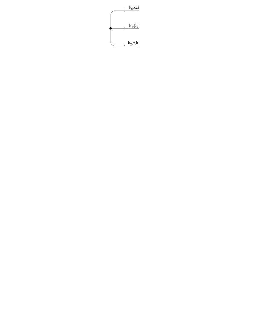
Figure 1: Initial proton state - three valence quarks with no soft gluons

Starting with three valence quarks, described by $\epsilon_{ijk}\psi^{(0)}(k_{0},k_{1},k_{2})$, we can calculate 1-soft gluon component of a proton wave function. Summing contributions of the three graphs in fig.2 we find (in the first order in strong coupling constant $g$):

$${\psi^{(1)}}^{~{}ijk~{}a_{1}}_{~{}~{}~{}~{}~{}\lambda_{1}}(k_{0},\dots k_{3})=i2\sqrt{2}g\frac{\bar{k}_{3}\cdot\bar{\epsilon}_{\lambda_{1}}}{\bar{k}_{3}^{2}}\left[\frac{\epsilon_{i^{\prime}jk}(T^{a_{1}})^{i}_{i^{\prime}}}{\sqrt{3!}}\psi^{(0)}(k_{0}+k_{3},k_{1},k_{2})\right.$$

$$\left.+\frac{\epsilon_{ij^{\prime}k}(T^{a_{1}})^{j}_{j^{\prime}}}{\sqrt{3!}}\psi^{(0)}(k_{0},k_{1}+k_{3},k_{2})+\frac{\epsilon_{ijk^{\prime}}(T^{a_{1}})^{k}_{k^{\prime}}}{\sqrt{3!}}\psi^{(0)}(k_{0},k_{1},k_{2}+k_{3})\right].$$ (3)

Here we have used a light-cone decomposition of the momenta, with $\bar{k}_{i}$ being the transverse component of $k_{i}$. It is convenient to work in a mixed momentum-space representation performing Fourier transform in $\bar{k}_{i}$. The corresponding 2-dimensional transverse position vectors are subsequently denoted by $x_{i}$, whereas $z_{i}$ correspond to the fractions of the “+” components of momenta with respect to the “+” component of the initial proton momentum. The details of the kinematics can be found in Ref.[5]. The 1-gluon component of the proton wave function takes the following form in the mixed momentum-space representation:

$${\psi^{(1)}}^{~{}ijk~{}a_{1}}_{~{}~{}~{}~{}~{}\lambda_{1}}({x}_{0},\dots{x}_{3};z_{0},\dots z_{3})=-\frac{\sqrt{2}}{\pi}g\psi^{(0)}({x}_{0},{x}_{1},{x}_{2};z_{0},z_{1},z_{2})$$

$$\left[\frac{\epsilon_{i^{\prime}jk}(T^{a_{1}})^{i}_{i^{\prime}}}{\sqrt{3!}}\frac{{x}_{30}\cdot\bar{\epsilon}_{\lambda_{1}}}{{x}_{30}^{2}}+\frac{\epsilon_{ij^{\prime}k}(T^{a_{1}})^{j}_{j^{\prime}}}{\sqrt{3!}}\frac{{x}_{31}\cdot\bar{\epsilon}_{\lambda_{1}}}{{x}_{31}^{2}}+\frac{\epsilon_{ijk^{\prime}}(T^{a_{1}})^{k}_{k^{\prime}}}{\sqrt{3!}}\frac{{x}_{32}\cdot\bar{\epsilon}_{\lambda_{1}}}{{x}_{32}^{2}}\right],$$ (4)

where $x_{ij}=x_{i}-x_{j}$ and $\bar{\epsilon}_{\lambda_{i}}$ is transverse part of gluon polarization vector.

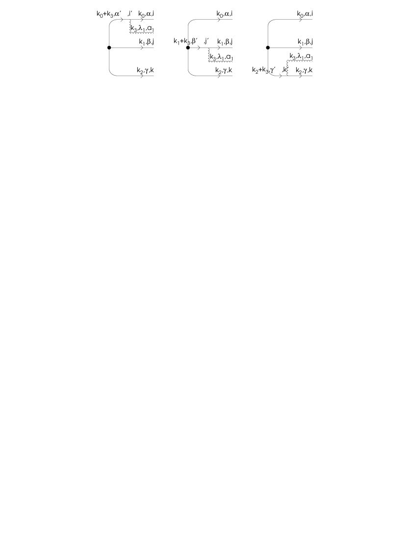
Figure 2: One gluon component of a proton wave function

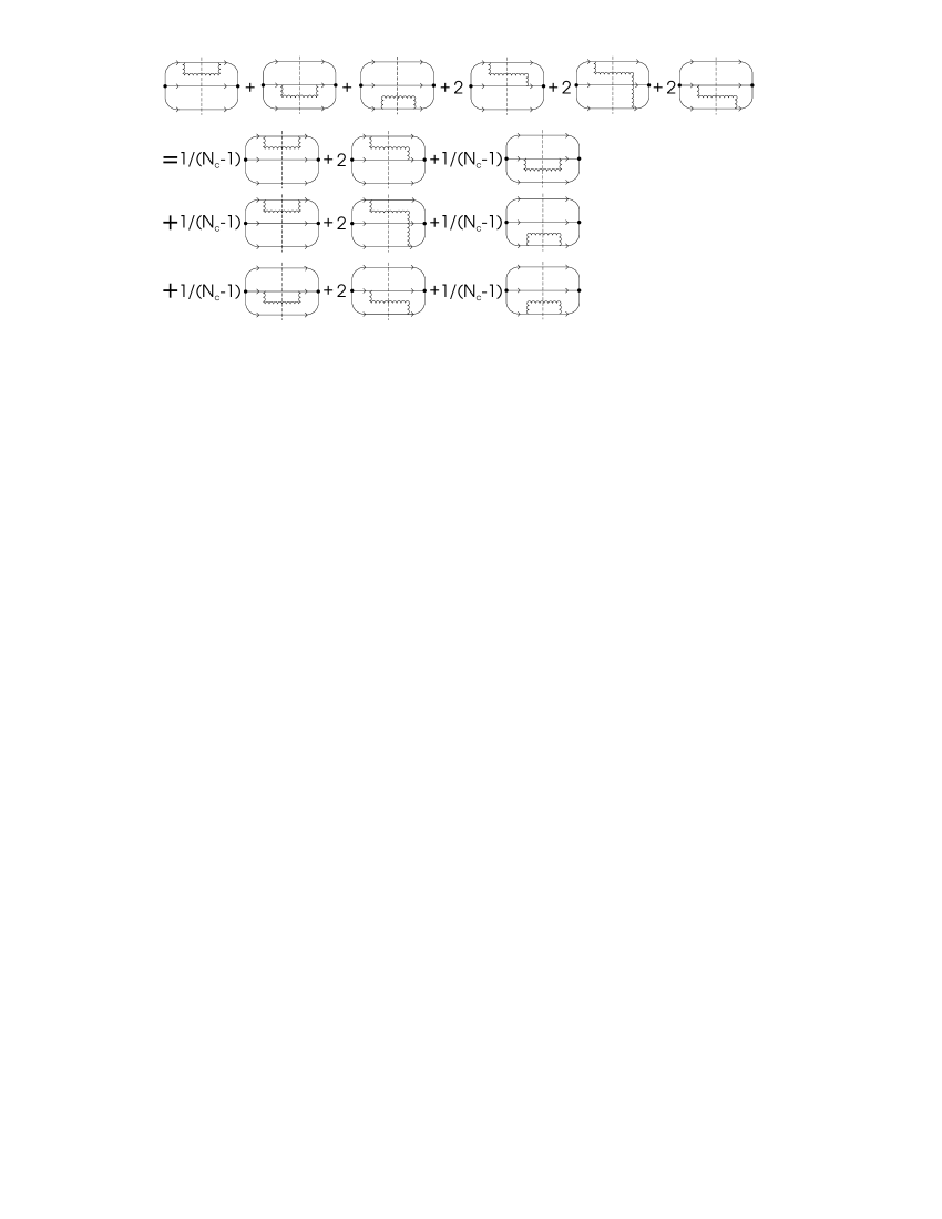
Figure 3: Square of the one gluon component of a proton wave function for $N_{\rm c}=3$

Now we can calculate $\Phi^{(1)}$ – square of the 1-gluon component of the proton wave function summed over gluon polarizations, which is depicted in the first row of fig.3. The color factor of the noninterference graphs (gluon emitted and absorbed by the same quark line – first three graphs of the first row of fig.3) equals $C_{F}$. The color factor of the interference graphs (gluon exchanged between the different quark lines – last three graphs of the first row of fig.3) equals $C_{F}/(N_{\rm c}-1)$. However we cannot neglect the interference diagrams, even in the large $N_{\rm c}$ limit. That is because in the large $N_{\rm c}$ limit a proton would be composed not from three but from $N_{\rm c}$ valence quarks. Therefore effectively each non-interference diagram has to be split into $(N_{\rm c}-1)$ ’copies’ in order to match the interference graphs. This is pictorially illustrated in fig.3 for $N_{\rm c}=3$. Each row in the second part of fig.3 sums up to a compact expression resembling a dipole production by an onium. Summing up the contribution from all 3 (or rather $N_{\rm c}(N_{\rm c}-1)/2$) rows we get:

$$\Phi^{(1)}({x}_{0},{x}_{1},{x}_{2},{x}_{3};z_{0},z_{1},z_{2},z_{3}) = \Phi^{(0)}({x}_{0},{x}_{1},{x}_{2};z_{0},z_{1},z_{2})$$ (5)

$$\frac{8\alpha_{\rm s}}{\pi}\frac{N_{\rm c}+1}{2N_{\rm c}}\,\left[\frac{x_{10}^{2}}{x_{30}^{2}x_{31}^{2}}+\frac{x_{20}^{2}}{x_{30}^{2}x_{32}^{2}}+\frac{x_{21}^{2}}{x_{31}^{2}x_{32}^{2}}\right].$$

It is important to note that interference diagrams make the integral:

$$\int\frac{d^{2}{x}_{3}}{2\pi}\Phi^{(1)}({x}_{0},\dots{x}_{3};z_{0},\dots z_{3})$$ (6)

IR finite (like in the dipole case). The UV divergence appears because the $virtual$ corrections have not been taken into account (see [5]) and the integral (6) should be appropriately regularized.

We can compare this result with the case of an onium.

$$\Phi_{\rm onium}^{(1)}({x}_{0},{x}_{1},{x}_{2};z_{0},z_{2},z_{3})=\Phi_{\rm onium}^{(0)}({x}_{0},{x}_{1};z_{0},z_{1})\frac{8\alpha_{\rm s}C_{F}}{\pi}\frac{x_{10}^{2}}{x_{20}^{2}x_{21}^{2}},$$ (7)

gives the universal probability of a gluon emission from a dipole. In the large $N_{\rm c}$ limit a gluon line can be represented as a quark-antiquark pair in color space. The onium with one gluon has then a straightforward interpretation of two dipoles and the probability (7) can be interpreted as a probability of a dipole (or equivalently an onium) splitting into two dipoles.

In the large $N_{\rm c}$ limit there is no interference between different dipoles, so once a gluon is emitted from one of the already existing dipoles we can again identify the resulting color structure as two new dipoles. Therefore the probability of emission of the second (or $n$-th) gluon is given by the sum of the probabilities of a gluon emission by two (or $n$) already existing dipoles. Thus for $\Phi^{(2)}_{\rm onium}$ we get an expression:

$$\Phi_{\rm onium}^{(2)}({x}_{0},\dots{x}_{3};z_{0},\dots z_{3}) = \Phi_{\rm onium}^{(0)}({x}_{0},{x}_{1};z_{0},z_{1})$$ (8)

$$\left(\frac{8\alpha_{\rm s}C_{F}}{\pi}\right)^{2}\frac{x_{10}^{2}}{x_{20}^{2}x_{21}^{2}}\left(\frac{x_{20}^{2}}{x_{30}^{2}x_{32}^{2}}+\frac{x_{21}^{2}}{x_{31}^{2}x_{32}^{2}}\right),$$

where the first factor ${x_{10}^{2}}/{x_{20}^{2}x_{21}^{2}}$ describes a process in which the original onium splits into 2 dipoles and the second term in brackets describes the splitting of these 2 dipoles into 2 new dipoles each. This pattern is universal at every order of $\alpha_{\rm s}$.

Similarly $\Phi^{(1)}$ of eq.(5) can be interpreted as a probability of an emission of the first soft gluon from a proton. Representing the first gluon as a quark-antiquark pair, one might try to interpret the resulting state as a proton made of two original quarks and a quark part of the gluon and a dipole made of an antiquark part of a gluon and the remaining quark of the original proton (fig.4a). In analogy with the onium case one could naturally expect that in the next step one would get:

1. a proton emitting the next gluon described by the kernel of eq.(5) and

2. a dipole emitting the next gluon described by the kernel of eq.(7).
Unfortunately it is not so.

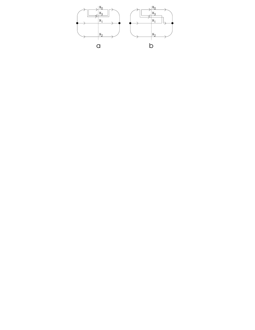
Figure 4: Large $N_{\rm c}$ limit of the first gluon emission

We shall show this by explicit calculation of the square of the proton wave function. We shall do this exactly, i.e. without escaping to the large $N_{\rm c}$ limit. The 2-gluon component of the proton wave function equals:

$${\psi^{(2)}}^{~{}ijk~{}a_{1}a_{2}}_{~{}~{}~{}~{}~{}\lambda_{1}\lambda_{2}}({x}_{0},\dots{x}_{4})=-\frac{\sqrt{2}}{\pi}g \left[(T^{a_{2}})^{i}_{i^{\prime}}{\psi^{(1)}}^{~{}i^{\prime}jk~{}a_{1}}_{\lambda_{1}}({x}_{0},\dots{x}_{3})\frac{{x}_{40}\cdot\bar{\epsilon}_{\lambda_{2}}}{{x}_{40}^{2}}\right.$$ (9)

$$+(T^{a_{2}})^{j}_{j^{\prime}}{\psi^{(1)}}^{~{}ij^{\prime}k~{}a_{1}}_{\lambda_{1}}({x}_{0},\dots{x}_{3})\frac{{x}_{41}\cdot\bar{\epsilon}_{\lambda_{2}}}{{x}_{41}^{2}}$$

$$+(T^{a_{2}})^{k}_{k^{\prime}}{\psi^{(1)}}^{~{}ijk^{\prime}~{}a_{1}}_{\lambda_{1}}({x}_{0},\dots{x}_{3})\frac{{x}_{42}\cdot\bar{\epsilon}_{\lambda_{2}}}{{x}_{42}^{2}}$$

$$\left.+if^{a_{1}a_{2}c}{\psi^{(1)}}^{~{}ijk~{}c}_{\lambda_{1}}({x}_{0},\dots{x}_{3})\frac{{x}_{43}\cdot\bar{\epsilon}_{\lambda_{2}}}{{x}_{43}^{2}}\right].$$

In order to calculate $\Phi^{(2)}$ it is convenient to split the entire expression into 2 parts. Contribution to $\Phi^{(2)}$ coming from the second gluon attached in all possible ways within a diagram of fig.4a equals:

$$\Phi^{(2)}_{4{\rm a}}({x}_{0},\ldots{x}_{4};z_{0},\ldots z_{4}) =\Phi^{(0)}({x}_{0},{x}_{1},{x}_{2};z_{0},z_{1},z_{2})\left(\frac{8\alpha_{\rm s}}{\pi}\right)^{2}{C_{F}}$$

$$\frac{1}{x_{30}^{2}}\left[\frac{N_{\rm c}}{2}\frac{x_{30}^{2}}{x_{43}^{2}x_{40}^{2}}+\frac{N_{\rm c}+1}{2N_{\rm c}}\left(\frac{x_{31}^{2}}{x_{43}^{2}x_{41}^{2}}+\frac{x_{32}^{2}}{x_{43}^{2}x_{42}^{2}}+\frac{x_{12}^{2}}{x_{41}^{2}x_{42}^{2}}\right)\right.$$

$$\left.+\frac{1}{2N_{\rm c}(N_{\rm c}-1)}\left(\frac{x_{31}^{2}}{x_{43}^{2}x_{41}^{2}}+\frac{x_{32}^{2}}{x_{43}^{2}x_{42}^{2}}-\frac{x_{01}^{2}}{x_{40}^{2}x_{41}^{2}}-\frac{x_{12}^{2}}{x_{41}^{2}x_{42}^{2}}\right)\right].$$

In this case the probability of the second gluon emission behaves as we would have a dipole ($x_{3}$, $x_{0}$), a proton ($x_{3}$, $x_{1}$, $x_{2}$) and a sum of four (or $2(N_{\rm c}-1)$) terms which in the large $N_{\rm c}$ limit can be neglected. However the prefactor $1/{x_{30}^{2}}$ corresponds only to one part of the emission kernel of the first gluon. Contribution to $\Phi^{(2)}$ coming from the second gluon attached in all possible ways within a diagram of fig.4b equals:

$$\Phi^{(2)}_{4{\rm b}}({x}_{0},\ldots{x}_{4};z_{0},\ldots z_{4}) =\Phi^{(0)}({x}_{0},{x}_{1},{x}_{2};z_{0},z_{1},z_{2})\left(\frac{8\alpha_{\rm s}}{\pi}\right)^{2}\frac{N_{\rm c}+1}{2N_{\rm c}}$$ (11)

$$\left(-2\frac{{x}_{30}\cdot{x}_{31}}{x_{30}^{2}x_{31}^{2}}\right)\left[\frac{N_{\rm c}}{2}\left(\frac{x_{03}^{2}}{x_{40}^{2}x_{43}^{2}}+\frac{x_{13}^{2}}{x_{41}^{2}x_{43}^{2}}-\frac{x_{01}^{2}}{x_{40}^{2}x_{41}^{2}}\right)\right.$$

$$\left.+\frac{N_{\rm c}+1}{2N_{\rm c}}\left(\frac{x_{01}^{2}}{x_{40}^{2}x_{41}^{2}}+\frac{x_{02}^{2}}{x_{40}^{2}x_{42}^{2}}+\frac{x_{12}^{2}}{x_{41}^{2}x_{42}^{2}}\right)\right].$$

In this case we get a color structure which cannot be identified with a proton and a dipole emitting a gluon. The probability of the second gluon emission behaves as we would have the original proton ($x_{0}$, $x_{1}$, $x_{2}$) and two dipoles ($x_{3}$, $x_{0}$ and $x_{3}$, $x_{1}$) with subtraction of another dipole ($x_{0}$, $x_{1}$). This is a signature of a new color structure. Here the prefactor corresponding to the first emission reads: $-2\;{x}_{30}\cdot{x}_{31}/{x_{30}^{2}x_{31}^{2}}$. The fact that even in the large $N_{\rm c}$ limit expressions in square brackets in eq.(2) and eq.(11) are different, makes it impossible to collect the prefactors into one compact expression like eq.(5).

To get the full expression for $\Phi^{(2)}$ one has to sum all (see fig.3) contributions from three (or $N_{\rm c}$) diagrams of the type of fig.4a, where the first gluon is emitted and absorbed by the same quark in the initial proton and from three (or $N_{\rm c}(N_{\rm c}-1)/2$) diagrams of the type of fig.4b, where the first gluon line extends between two different quark lines of the original proton. On the top of the first gluon the second gluon line should be added accordingly. Thus one gets:

$$\Phi^{(2)}({x}_{0},\dots,{x}_{4};z_{0},\dots z_{4})=$$

$$\Phi^{(2)}_{4{\rm a}}({x}_{0},{x}_{1},{x}_{2},{x}_{3},{x}_{4};z_{0},\ldots z_{4})+\Phi^{(2)}_{4{\rm a}}({x}_{1},{x}_{0},{x}_{2},{x}_{3},{x}_{4};z_{0},\ldots z_{4})+\Phi^{(2)}_{4{\rm a}}({x}_{2},{x}_{1},{x}_{0},{x}_{3},{x}_{4};z_{0},\ldots z_{4})+$$

$$\Phi^{(2)}_{4{\rm b}}({x}_{0},{x}_{1},{x}_{2},{x}_{3},{x}_{4};z_{0},\ldots z_{4})+\Phi^{(2)}_{4{\rm b}}({x}_{0},{x}_{2},{x}_{1},{x}_{3},{x}_{4};z_{0},\ldots z_{4})+\Phi^{(2)}_{4{\rm b}}({x}_{1},{x}_{2},{x}_{0},{x}_{3},{x}_{4};z_{0},\ldots z_{4})$$

Although the full expression is IR finite there is no factorization of the first gluon emission as given by eq.(5). It seems to us that this might be due to the fact that at every step of the gluon cascade new color structures appear which cannot be reduced to one proton and a number of dipoles.

3 Diquark limit and dipole equation

It is not clear to us whether the assumption, made in Refs.[8, 9], that up to a normalization factor there is no difference between a proton and an onium soft gluon dynamics can be justified in general case. However, if we assume that two valence quarks are localized in the same transverse position we recover the dipole equation. This is is of course an expected feature, since two (or $N_{\rm c}-1$) quarks in antisymmetric state behave like an antiquark.

It is, however, instructive to check this on the example of $\Phi^{(2)}$. Putting ${x}_{1}={x}_{2}$ in the expression (2) for $\Phi^{(2)}$ and remembering about combinatory factors we get:

$$\Phi^{(2)}({x}_{0},{x}_{1}={x}_{2},{x}_{3},{x}_{4};z_{0},\dots z_{4}) =\Phi^{(0)}({x}_{0},{x}_{1}={x}_{2};z_{0},z_{1},z_{2})\left(\frac{8\alpha_{\rm s}}{\pi}\right)^{2}C_{F}$$

$$\frac{x_{10}^{2}}{x_{30}^{2}x_{31}^{2}}\left[\frac{N_{\rm c}}{2}\left(\frac{x_{30}^{2}}{x_{43}^{2}x_{40}^{2}}+\frac{x_{31}^{2}}{x_{43}^{2}x_{41}^{2}}\right)-\frac{1}{2N_{\rm c}}\frac{x_{01}^{2}}{x_{40}^{2}x_{41}^{2}}\right],$$

which in the large $N_{\rm c}$ limit reduces to (8).

4 Summary

In this short note we have calculated two soft gluon contribution to the wave function of the proton. The first gluon emission, described by eq.(5), reveals all nice features of the onium case:

1. it is IR finite and

2. can be interpreted as dipole emission from the initial proton.
One has to stress that this result can be obtained only if the interference diagrams of the type of fig.4b are included. With respect to the graphs of the type of fig.4a their color factor is suppressed as $1/N_{\rm c}$, however, their number grows like $N_{\rm c}$ and therefore they cannot be neglected.

The emission of the next gluon causes the problem. Kinematical factors in transverse configuration space corresponding to diagrams of fig.4a and fig.4b are completely different. In fact the naive interpretation, that in the first emission the proton splits into a dipole and another proton breaks down. Instead we encounter new color structures, like the one in fig.4b, where the quark and antiquark lines which are localized in the same transverse position are interchanged many times. This is perhaps the signature that some new color structures, not only dipoles and three-quark singlets (like proton) appear. However, we do not have any solid proof of this statement at the moment.

We have also checked by explicit calculation that if 2 (or $N_{\rm c}-1$) quarks are “by force” put into the same transverse position the dipole equation emerges. This is an expected feature, since two (or $N_{\rm c}-1$) quarks in antisymmetric state behave like an antiquark.

Acknowledgements

We would like to thank A. Białas for suggesting this investigation and useful discussions and R. Peschanski for discussions. The authors acknowledge the support of Polish KBN Grant PB 2 PO3B 044 12. M.P. acknowledges support of A. v. Humboldt Foundation.

References

- [1] Ya. Ya. Balitsky, L. N. Lipatov, Sov. J. Nucl. Phys. 28 (1978) 822.
- [2] E. A. Kuraev, L. N. Lipatov, V. S. Fadin, Sov. Phys. JETP 45 (1977) 199
- [3] L. N. Lipatov, Sov. Phys. JETP 63 (1986) 904
- [4] N. Nikolaev, B.G. Zaharkov, Phys. Lett. B 327 (1994) 149
- [5] A.H. Mueller, Nucl. Phys. B 415 (1994) 373
- [6] A.H. Mueller, B. Patel, Nucl. Phys. B 425 (1994) 471, hep-ph/9403256
- [7] Z Chen, A.H. Mueller, Nucl. Phys. B 451 (1995) 579
- [8] H. Navelet, R. Peschanski, Ch. Royon, Phys. Let. B 366 (1996) 329, hep-ph/9508259
- [9] H. Navelet, R. Peschanski, Ch. Royon, S. Wallon, Phys. Let. B 385 (1996) 357, hep-ph/9605389
- [10] A. Białas, W. Czyż, W. Florkowski, Phys.Rev. D55 (1997) 6830, hep-ph/9701209
- [11] A. Białas, W. Czyż, W. Florkowski, hep-ph/9705470
- [12] A. Białas, R. Peschanski, Phys.Lett.B355 (1995) 301, hep-ph/9504293 and Phys.Lett.B378 (1996) 302, hep-ph/9512427
- [13] A. Białas, Acta Phys.Polon. B27 (1996) 1263