Multibody neutrino exchange in a neutron star:
neutrino sea and border effects

Abstract

The interaction due to the exchange of massless neutrinos between neutrons is a long-range force. Border effects on this multibody exchange inside a dense core are studied and computed analytically in $1\ +\ 1$ dimensions. We demonstrate in this work that a proper treatment of the star’s border effect automatically incorporates the condensate contribution as a consequence of the appropriate boundary conditions for the neutrino Feynman propagator inside the star. The total multibody exchange contribution is infrared-safe and vanishes exactly in $1\ +\ 1$ dimensions. The general conclusion of this work is that the border effect does not modify the result that neutrino exchange is infrared-safe. This toy model prepares the ground and gives the tools for the study of the realistic $3\ +\ 1$ star.

December 1997

The possible connection between the multibody neutrino exchange and the stability of compact stellar objects has recently motivated several relevant works [1]–[4]. The interest raised by Fischbach’s original idea [1] is based on the presumably catastrophic consequences for the self-energy of compact objects, such as neutron stars, originated by the long-range neutron correlation due to massless neutrino exchange. This catastrophic effect is then invoked to justify the introduction of a lower bound for the neutrino mass. In a previous work [2], we have shown that the total contribution of the many-body massless neutrino exchanges may be directly and rather easily computed, using an effective Lagrangian, and results in an infrared well-behaved star self-energy. The catastrophic result of the resummation method is simply due, in our opinion, to the fact that it is done outside the radius of convergence of the perturbative series.

Smirnov and Vissani [3], following Fischbach’s approach of summing up many-body exchange, order by order, showed that the 2-body potential is damped by the blocking effects of the neutrino sea [6] and conjectured that a similar effect for a many-body potential would reduce Fischbach’s catastrophic effect.

The effect of such a condensate has also been incorporated in our non-perturbative method by using a neutrino Feynman propagator inside a dense stellar medium with a condensate term [2]. However, this condensate does not bring any major modification to our conclusion that the total result of the multi-body massless neutrino exchange is infrared well-behaved.

The objection to our previous work [5] is that we had worked in the approximation where the presence of the neutron star border was negligible. In fact, we stressed in [2] our belief that the neutrino condensate had to be understood as a manifestation of the star’s border, and a preliminary proof of that statement can be found in ref. [4].

In this paper, we shall demonstrate that a proper treatment of the star’s border effect automatically incorporates the condensate contribution. And that this is a consequence of the appropriate boundary conditions for the Feynman propagator of the massless neutrino in the interacting medium. Finally, we will show that the border effect does not modify our main result that neutrino exchange is infrared-safe.

Our tool in this proof is the computation of the Feynman propagator for the massless neutrino in the neutron star medium. In [2], ignoring the border effect and hence using the translational symmetry, we have found the following effective propagator

$${i\over\hbox to0.0pt{/\hss}q-b\gamma^{0}}\ \ ,$$ (1)

where $b\gamma^{0}$ accounts for $Z^{0}$-exchange diagrams between the neutrino and the neutrons of the medium in the static limit.

The latter is an infrared regular propagator, which can be written as follows:

$${i\over\hbox to0.0pt{/\hss}q-b\gamma^{0}}={i\hbox to0.0pt{/\hss}q_{>}\over q_{>}^{2}+is\varepsilon}\ \ ,$$ (2)

where $(q_{>})^{\mu}=(q_{0}-b,\vec{q})$. The term $is\varepsilon$ is the infrared regulator, where $s$ is a sign that stands for the appropriate “time convention”. The determination of $s$ needs some care: the propagator has been rewritten in terms of the four-momentum $q_{>}$, its “time” component being $(q_{0}-b)$ instead of $q_{0}$. As we will show, the appropriate boundary conditions, i.e. the “time convention”, should be imposed to keep the usual distribution in the $q_{0}$ complex plane of the poles for the Feynman propagator: since neutrino (antineutrino) states correspond to the positive energy (the hole of negative energy) solutions, then the positive (negative) energy propagates forward (backward) in time. This rule implies

$$s=\mbox{sign}(q_{0})\mbox{sign}(q_{0}-b)\ \ .$$ (3)

It is crucial to insist that by energy we here meanstrictly $q_{0}$ and not the combination $(q_{0}-b)$, which expresses the distance of the energy level to the bottom of the potential $V\equiv b$. As a consequence, $b$ being negative, we get these dispersion relations for neutrinos and antineutrinos:

$$\begin{array}[]{ll}E_{\nu}=q_{0}=|\vec{q}|+b\ \ \ \quad\quad\ \ \ \ \mbox{for}\ |\vec{q}|>|b|\\ E_{\overline{\nu}}=-q_{0}=\left\{\begin{array}[]{ll}|\vec{q}|-b&\quad\forall|\vec{q}|\ \ \ \mbox{or}\ ,\\ -|\vec{q}|-b&\ \ \ \mbox{for}\ |\vec{q}|<|b|\end{array}\right.\end{array}$$ (8)

Finally, the poles are in the first and/or third quadrants in $q_{0}$ complex plane, as shown in fig. 1. Had we taken $s=1$, for a range of values of $|\vec{q}|<|b|$ poles would have appeared in the other quadrants (see fig. 1). Such a pole should be taken into account when rotating to Euclidean time. This has not been done correctly in [2], inducing a minor error which will be discussed below.

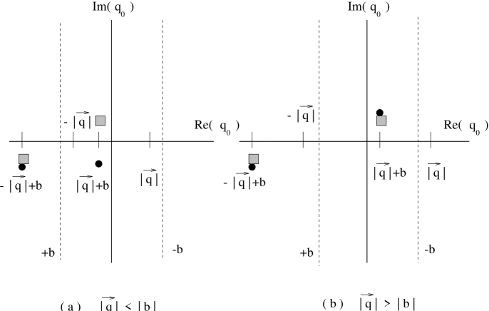
FIG. 1.: Schematic distribution of the poles of the propagator. The black dots and the grey squares represent the poles placed by following the time convention $is\varepsilon$ and $+i\varepsilon$, respectively.

Let us now return to the central issue of this note, which is the estimation of the border effect. As an attempt to have a simple analytic result, we start, in this work, our study with the $1\ +\ 1$ dimensions toy model for the following reasons: i) we will be able to work analytically to the end, ii) the subtle problem of the $i\varepsilon$ convention is easier to master,
iii) thanks to the relative simplicity of the problem, we will be able to use different complementary techniques and to get a deeper understanding of the physics, which will prove most helpful for a more realistic problem, i.e. $3\ +\ 1$ dimensions [10].

For simplicity, we consider a sharp border located at $z=0$ and use an effective neutrino Lagrangian that summarizes the interaction with the neutrons [4]:

$${\cal L}_{eff}=i{\overline{\nu}}(x)\hbox to0.0pt{/\hss}\partial\nu(x)-b\theta(z){\overline{\nu}}(x)\gamma^{0}\nu(x)\ \ ,$$ (9)

where $b\sim-\sqrt{2}G_{F}{n_{n}\over 2}\sim-0.2\times 10^{-7}{\mbox{GeV}}$, $n_{n}$ being the neutron density of the star [2].

The usual definition of the propagator is the following:

$$S_{F}(x,y)=\langle 0|T\left(\Psi(x)\overline{\Psi}(y)\right)|0\rangle\ \ .$$ (10)

It is worth stressing at this point that the time-ordered product will give us the Feynman boundary conditions.

Following Gavela et al. [8], $\Psi(x)$, the general Dirac solution of the problem, can be written as:

$$\Psi(x)=\sum_{\pm\vec{k},h}b_{h}(\pm\vec{k})\nu^{h}_{\pm\vec{k}}(\vec{x})e^{-iEt}\ +\ d^{{\dagger}}_{h}(\pm\vec{k})\nu^{A\ h}_{\pm\vec{k}}(\vec{x})e^{iEt}\ \ ,$$ (11)

where $\nu$ are the eigenstates of the Dirac Hamiltonian derived from the Lagrangian (9). In the second quantization, the coefficients $b$ and $d^{{\dagger}}$ become annihilation and creation operators, respectively.

The functions $\nu$ can be obtained from the following complete set of solutions:

$$\nu_{\pm{\vec{k}}}^{h}(z,t)=e^{-iE(t\mp z)}u_{h}(\pm{\vec{k}})\left\{\theta(-z)+e^{\mp ibz}\theta(z)\right\}\ \ ,$$ (12)

$$\nu_{\pm{\vec{k}}}^{A\ h}(z,t)=e^{iE(t\mp z)}v_{h}({\pm\vec{k}})\left\{\theta(-z)+e^{\mp ibz}\theta(z)\right\}\ \ \ ,$$ (13)

which are obtained by solving the equation of motion for the $1\ +\ 1$ Lagrangian of eq. (9),

$$\left\{\gamma^{0}\left(i\partial_{t}-b\theta(z)\right)+i\gamma^{1}\partial_{1}\right\}\nu({\vec{x}},t)=0\ \ .$$ (14)

In eq. (13), the index $h$ expresses the chirality of the solution and $A$ denotes the antiparticles. Note that the chirality is the same on both sides of the border, as expected from the chirality-conserving Lagrangian of eq. (9).

In the region $z>0$ (inside the star), neutrinos have $k_{z}=\pm(E-b)$ and antineutrinos have $k_{z}=\pm(E+b)$, while in the region $z<0$ (outside the star), they have both $k_{z}=\pm E$. The subscripts $\pm{\vec{k}}$ depend on the choice of the sign for $k_{z}$. In Eq. (13) $u$ and $v$ are the Dirac spinors for particles and antiparticles, respectively,

$$\hbox to0.0pt{/\hss}k_{>,<}^{\pm}\left\{\begin{array}[]{r}u_{h}(\pm\vec{k})\\ v_{h}(\pm\vec{k})\end{array}\right\}\ =\ 0\ ,$$ (17)

where $k_{>}^{\pm}=(E-b,\pm(E-b))$ for neutrinos, $k_{>}^{\pm}=(E+b,\pm(E+b))$ for antineutrinos and $k_{<}^{\pm}=(E,\pm E)$ for both.

Equations (11) and (13) imply a definite choice of the zero energy level that corresponds to the standard choice of the free neutrinos far outside the star, $z\to-\infty$, clearly the only admissible choice. Physically this choice is related to the use of a stationary Lagrangian, (9), which means that we assume that the system has relaxed to equilibrium, implying plane-wave solutions that extend outside and inside the star. These plane waves “know” the zero energy level from their outer domain. This choice, combined with the time-ordered product of eq. (10), implies the $+is\varepsilon$ time regulator in momentum space as announced before.

In momentum space, the propagator can be written as

$$\begin{array}[]{l}S_{F}(q^{f},q^{i})\gamma^{0}={i\over 2\pi}\int_{0}^{\infty}dk_{0}\left[\widetilde{\nu_{\pm\vec{k}}^{h}(q_{z}^{f})}\left(\widetilde{\nu_{\pm\vec{k}}^{h}(q_{z}^{i})}\right)^{{\dagger}}{1\over q_{0}-k_{0}+i\varepsilon}\right.\\ \left.+\ \widetilde{\nu_{\pm\vec{k}}^{A\ h}(q_{f}^{f})}\left(\widetilde{\nu_{\pm\vec{k}}^{A\ h}(q_{z}^{i})}\right)^{{\dagger}}{1\over q_{0}+k_{0}-i\varepsilon}\right]\ \ \ ,\end{array}$$ (20)

where $q^{f,i}=(q_{0},q_{z}^{f,i})$. Notice that the character of creation or annihilation for the operators in eq. (11) is fixed by taking the matter-free vacuum as reference, i.e. it is a consequence of our choice of the zero energy level. $\widetilde{\nu}$ are the Fourier transform of the eigenstates $\widetilde{\nu(q_{z})}=\int_{-\infty}^{+\infty}dz\ e^{-iq_{z}z}\nu(z)$:

$$\widetilde{\nu_{\pm{\vec{k}}}^{h}(q_{z})}=i\left({1\over q_{z}\mp k_{0}+i\varepsilon}-{1\over q_{z}\mp(k_{0}-b)-i\varepsilon}\right)u_{h}(\mp{\vec{k}})\ \ ,$$ (21)

$$\widetilde{\nu_{\pm{\vec{k}}}^{A\ h}(q_{z})}=i\left({1\over q_{z}\pm k_{0}+i\varepsilon}-{1\over q_{z}\pm(k_{0}+b)-i\varepsilon}\right)v_{h}(\pm{\vec{k}})\ \ .$$ (22)

We took $E=k_{0}$ in order to make the notation uniform. Applying this last result in eq. (20), with the appropriate analytic continuation of the integration variable $k_{0}$, and by following the adequate integration contour (see appendix Multibody neutrino exchange in a neutron star: neutrino sea and border effects), we obtain for the $1\ +\ 1$ propagator:

$$\begin{array}[]{l}S_{F}(q^{f},q^{i})=2\pi\delta\left(q_{z}^{f}-q_{z}^{i}\right){i\over(\hbox to0.0pt{/\hss}q_{>})^{*}}\ +\ {b\over 2}\ {1\over q_{z}^{f}-q_{z}^{i}+i\varepsilon}\\ \times\left\{{1\over(\hbox to0.0pt{/\hss}q_{>}^{i})^{*}}\gamma^{0}{1\over\hbox to0.0pt{/\hss}q_{<}^{f}}\left(1+\mbox{sign}(q_{0})\alpha_{z}\right)\right.\left.+{1\over(\hbox to0.0pt{/\hss}q_{>}^{f})^{*}}\gamma^{0}{1\over\hbox to0.0pt{/\hss}q_{<}^{i}}\left(1-\mbox{sign}(q_{0})\alpha_{z}\right)\right\}\ \ ,\end{array}$$ (25)

where we define:

$${1\over\hbox to0.0pt{/\hss}q_{<}}={1\over\hbox to0.0pt{/\hss}q}={\hbox to0.0pt{/\hss}q_{<}\over q_{<}^{2}+i\varepsilon}\ \mbox{with}\ \ \left(q_{<}\right)^{\mu}=q^{\mu}=(q_{0},{\vec{q}})\ \ ,$$ (26)

$${1\over(\hbox to0.0pt{/\hss}q_{>})^{*}}={\hbox to0.0pt{/\hss}q_{>}\over q_{>}^{2}+is\varepsilon}\ \mbox{with}\ \ \left(q_{>}\right)^{\mu}=(q_{0}-b,{\vec{q}})\ \ ,$$ (27)

with $s=\mbox{sign}(q_{0})\mbox{sign}(q_{0}-b)$ and $\alpha_{z}=\gamma^{0}\gamma^{1}$. The location of the poles in the complex plane have already been depicted in fig. 1.

Anticipating over the vacuum energy calculation, it is interesting to notice that the second term in the r.h.s of eq. (25) does not contribute when the border is sent to infinity; one is then left with only the first term, which is exactly the one of eq. (2) for the infinite star with the same good regularization. To convince ourselves, eq. (25) can be rewritten as follows:

$$\begin{array}[]{l}S_{F}(q^{f},q^{i})=2\pi i\delta\left(q_{z}^{f}-q_{z}^{i}\right)\left\{{1\over(\hbox to0.0pt{/\hss}q_{>})^{*}}-{b\over 2}{1\over(\hbox to0.0pt{/\hss}q_{>})^{*}}\gamma^{0}{1\over\hbox to0.0pt{/\hss}q_{<}}\right\}\\ +{b\over 2}{\cal P}\left({1\over q_{z}^{f}-q_{z}^{i}}\right)\left\{{1\over(\hbox to0.0pt{/\hss}q_{>}^{i})^{*}}\gamma^{0}{1\over\hbox to0.0pt{/\hss}q_{<}^{f}}-{1\over(\hbox to0.0pt{/\hss}q_{>}^{f})^{*}}\gamma^{0}{1\over\hbox to0.0pt{/\hss}q_{<}^{i}}\right\}\mbox{sign}(q_{0})\alpha_{z}\ \ ,\end{array}$$ (30)

where ${\cal P}$ stands for the principal value. For an observer located at $z\to\infty$, which means that he does not see the star border, restoring the translational symmetry, i.e. $q_{z}^{f}\to q_{z}^{i}$ (when $z\to\infty$), is a good approximation. Consequently, the second term in the r.h.s of eq. (30) will not contribute when $z\to\infty$ . Furthermore, it can be seen from eq. (34) below that after the integration over the momenta, as suggested by Schwinger’s method to obtain the vacuum energy, the second term in the r.h.s of eq. (25) does not contribute to the energy density $w(z\to+\infty)$.

The expression for $1/(\hbox to0.0pt{/\hss}q)^{*}$, given by eq. (27), can be appropriately rewritten as

$${i\over(\hbox to0.0pt{/\hss}q_{>})^{*}}=i\left\{{1\over\hbox to0.0pt{/\hss}q_{>}}+2\pi i\hbox to0.0pt{/\hss}q_{>}\delta\left(q_{>}^{2}\right)\theta(q_{0})\theta(b-q_{0})\right\}\ \ .$$ (31)

This last equation is a concrete demonstration that we have, in $1\ +\ 1$ dimensions, generated the condensate contribution in a natural way to all orders. In refs. [2] and [3], the same condensate term in the r.h.s of eq. (31) was introduced by hand. We should stress that in ref. [2] we initially computed the weak energy density by using the $+i\varepsilon$ convention (first term of eq. (31)), but we did not take into account the pole $q_{0}=|\vec{q}|+b$, in the second quadrant for $|\vec{q}|<|b|$ (see fig. 1) when rotating to Euclidean time. This explains our non-zero result for the energy density when we have fixed the good boundary conditions by introducing the second term of eq. (25) for the propagator.

The existence of a certain neutrino condensate due to the interaction of neutrinos and the stellar matter background was initially proposed by Loeb [6]: neutrinos are trapped inside the star and antineutrinos are repelled. The relevant physics concerning the neutrino propagator in the scenario we described above would appear by introducing the appropriate boundary conditions. Equations (27) and (31) give a confirmation of the idea proposed in ref. [2]: the condensate is a consequence of the existence of a border.

This condensate is physically understandable. As we have tuned the level of the Dirac sea outside the star (to the left) and as our states extend over all space, far inside the star (to the right), the level corresponds to filling a Fermi sea above the bottom of the potential $b<q_{0}<0$. This obviously induces a Pauli blocking effect. Equation (8) anticipates this result: $|b|$ is a lower bound for the momentum of the $q_{0}$-positive states.

With these tools, let us compute the total neutrino-exchange contribution to the energy of the star, which is nothing else than the difference between the vacuum energy of our effective theory eq. (9) and the vacuum energy of free neutrinos (without the star). Following Schwinger’s method [7], the vacuum energy in the presence of an external field is given by tracing the Hamiltonian multiplied by the propagator, as done in refs. [1] and [2]. Now, we compute the time-independent vacuum energy density

$$\begin{array}[]{l}w(z)\equiv-{i}\partial_{t}\mbox{tr}[\gamma^{0}\left(S_{F}(z,t;z^{\prime},t)-S^{(0)}_{F}(z,t;z^{\prime},t)\right)P_{L}]_{z^{\prime}\to z}\\ =\int{dq_{z}^{f}\ dq_{z}^{i}\ dq_{0}\over(2\pi)^{3}}\ \mbox{tr}\left[q_{0}\gamma^{0}e^{i(q_{z}^{f}-q_{z}^{i})z}\left(S_{F}(q^{f},q^{i})-S_{F}^{(0)}(q^{f},q^{i})\ 2\pi\delta\left(q_{z}^{f}-q_{z}^{i}\right)\right)P_{L}\right]\ \ ,\end{array}$$ (34)

where $S^{(0)}_{F}$ is the free neutrino propagator and $P_{L}={1-\gamma_{5}\over 2}$. We should remark that the $e^{i(q_{z}^{f}-q_{z}^{i})z}$ in the second line of this equation is generated by the break-up of the translational symmetry due to the border.

Now, by applying the expression of eq. (25) for the propagator in this last equation, we obtain:

$$w(z)\ =-\int\ {dq_{z}\ dq_{0}\over(2\pi)^{2}}\mbox{tr}\left[q_{0}\gamma^{0}\left({i\over(\hbox to0.0pt{/\hss}q_{>})^{*}}-{i\over\hbox to0.0pt{/\hss}q_{<}}\right)P_{L}\right]$$ (35)

$$-{b\over 2}\int\ {dq_{z}^{f}\ dq_{z}^{i}\ dq_{0}\over(2\pi)^{3}}\ {1\over q_{z}^{f}-q_{z}^{i}+i\varepsilon}\times$$ (36)

$$\mbox{tr}\left[e^{i(q_{z}^{f}-q_{z}^{i})z}\left\{{1\over(\hbox to0.0pt{/\hss}q_{>}^{i})^{*}}\gamma^{0}{1\over\hbox to0.0pt{/\hss}q_{<}^{f}}\left(1+\mbox{sign}(q_{0})\alpha_{z}\right)\right.\right.\left.\left.+{1\over(\hbox to0.0pt{/\hss}q_{>}^{f})^{*}}\gamma^{0}{1\over\hbox to0.0pt{/\hss}q_{<}^{i}}\left(1-\mbox{sign}(q_{0})\alpha_{z}\right)\right\}P_{L}\right]\ \ .$$ (37)

It should be noted that the first term of the r.h.s can be appropriately rewritten by using the Schwinger–Dyson relation, which has been shown in ref. [2] for the effective propagator (1) in the case of the infinite star . However, the calculation is rather cumbersome, even if it presents no special difficulty and leads to the amazing result:

$$w(z)=0\ .$$ (38)

As surprising as this result may seem, it can be understood physically in a rather simple way. One must remember [7] that $w(z)$ is nothing else than:

$$\sum\!\!\!\!\!\!\!\int_{n_{-}}E_{n_{-}}\Psi^{{\dagger}}_{n_{-}}(z)\Psi_{n_{-}}(z)-\sum\!\!\!\!\!\!\!\int_{n_{-}}E^{(0)}_{n_{-}}\Psi^{{\dagger}(0)}_{n_{-}}(z)\Psi^{(0)}_{n_{-}}(z)\ \ ,$$ (39)

where $n_{-}$ labels the negative energy states and $(0)$ refers to the matter-free vacuum.

These integrals are ultraviolet-divergent and we will allow the interchange of the sum and the integral as a regularization method. This was implicitly done in eq. (37). Looking now at the solutions of eq. (13) of the Hamiltonian with and without ($b=0$) the star, we first that remark there is a one-to-one correspondance of the states in the two situations and with the same energy; furthermore the probability density of the states are all equal to 1 for all $z$. More explicitly, the border does not disturb the wave functions, except for a phase. Consequently, after regularization (interchanging the sum and the difference) each term in the sum of eq. (39) vanishes.

The ($1\ +\ 1$)-dimensional problem presents the particularity that, for a given wave-plane solution, the sign of the momentum determines a positive correspondence between $z=\ +\ (-)\infty$ and $t=\ +\ (-)\infty$, or vice versa. Massless fermions are not reflected by a one-dimensional potential. However, the potential introduced through the Lagrangian (9) does not allow us to identify, for a given process, asymptotically free states for $t=\pm\infty$, because there is no “vacuum” to the right, and hence the S-matrix formalism is not adequate in a world defined by such a Lagrangian. In order to avoid the latter, we can take a second border. In this case, one can easily see that the phase shift taken by the neutrino states keeps the S-matrix diagonal: the star is “transparent” for the neutrino propagation. Therefore, by applying eq. (39), we can now conclude that the diagonality of the S-matrix justifies the null result for the weak energy density .

The generalization to the ($3\ +\ 1$)-dimensional problem is difficult even if the border is simplified to a flat one because of the presence of a refraction index, of a consequent modification of the probability density of the waves at the border, including non-penetrating or non-outgoing waves. This ($3\ +\ 1$)-dimensional problem will be analytically and numerically studied in a forthcoming work [10].

However, two main conclusions of this paper will remain valid in $3\ +\ 1$ dimensions:
i) the natural connection between the neutrino sea and the border, ii) the proper definition of the $is\epsilon$ infrared regulator for the propagator, or, equivalently, the correct definition of the zero energy level of the Dirac sea. On the other hand, the vanishing of the energy density $w(z)$ will not remain valid in $3\ +\ 1$ dimensions.

Finally, this work is a confirmation of the conclusion of ref. [2]: after correcting the mistake of forgetting the pole in the analytic continuation, and adding the condensate, which is proved here to be directly connected to the border, the multibody exchange of massless neutrinos results in an infrared-well -behaved contribution for the neutron star self-energy.

Acknowledgements

This work has been partially supported by Spanish CICYT, project PB 95-0533-A. We are specially grateful to B. M. Gavela for the discussions that initiated this work. A. Abada thanks A. Smirnov for inspiring discussion. J. Rodríguez–Quintero thanks M. Lozano for many important and helpful discussions and comments.

Details of integration in $1\ +\ 1$ dimensions

To compute the Feynman neutrino propagator in the momentum space, we should apply the results for the Fourier-transformed eigenstates (22) in eq. (20). After some tedious transformations, we obtain:

$${i\over 2\pi}\int_{0}^{+\infty}dk_{0}\left(I_{1}+I_{2}+I_{3}+I_{4}\right)\ \ ,$$ (40)

where

$$\begin{array}[]{l}I_{1}={1\over{1\over b}\left(q_{z}^{f}-k_{0}\right)\left(q_{z}^{f}-k_{0}+b\right)+i\varepsilon}\times\\ \\ {1\over{1\over b}\left(q_{z}^{i}-k_{0}\right)\left(q_{z}^{i}-k_{0}+b\right)-i\varepsilon}\ {1\over 2}\left(\gamma^{0}-\gamma^{1}\right)\gamma^{0}{1\over q_{0}-k_{0}+i\varepsilon}\ \ ,\\ \\ I_{2}={1\over-{1\over b}\left(q_{z}^{f}+k_{0}\right)\left(q_{z}^{f}+k_{0}-b\right)+i\varepsilon}\times\\ \\ {1\over-{1\over b}\left(q_{z}^{i}+k_{0}\right)\left(q_{z}^{i}+k_{0}-b\right)-i\varepsilon}\ {1\over 2}\left(\gamma^{0}+\gamma^{1}\right)\gamma^{0}{1\over q_{0}-k_{0}+i\varepsilon}\ \ ,\\ \\ I_{3}={1\over{1\over b}\left(q_{z}^{f}+k_{0}\right)\left(q_{z}^{f}+k_{0}+b\right)+i\varepsilon}\times\\ \\ {1\over{1\over b}\left(q_{z}^{i}+k_{0}\right)\left(q_{z}^{i}+k_{0}+b\right)-i\varepsilon}\ {1\over 2}\left(\gamma^{0}-\gamma^{1}\right)\gamma^{0}{1\over q_{0}+k_{0}-i\varepsilon}\ \ ,\\ \\ I_{4}={1\over-{1\over b}\left(q_{z}^{f}-k_{0}\right)\left(q_{z}^{f}-k_{0}-b\right)+i\varepsilon}\times\\ \\ {1\over-{1\over b}\left(q_{z}^{i}-k_{0}\right)\left(q_{z}^{i}-k_{0}-b\right)-i\varepsilon}\ {1\over 2}\left(\gamma^{0}+\gamma^{1}\right)\gamma^{0}{1\over q_{0}+k_{0}-i\varepsilon}\ \ .\end{array}$$ (56)

By taking into account the form of the different expressions for $I_{i}$ in eqs. (56), we have:

$$\int_{0}^{\infty}dk_{0}\left(I_{1}+I_{3}\right)=\int_{C_{1}}dk_{0}I_{1}\ \ ,$$ (57)

$$\int_{0}^{\infty}dk_{0}\left(I_{2}+I_{4}\right)=\int_{C_{1}}dk_{0}I_{2}\ \ ,$$ (58)

where the integration in the r.h.s should be done in the complex plane by following the contour $C_{1}$ (see fig. 2).

FIG. 2.: Integration contour $C_{1}$. (a) $q_{0}>0$ case; (b) $q_{0}<0$ case.

Identifying the relevant poles for each case and applying Cauchy’s theorem, we obtain the $1\ +\ 1$ propagator given above by eq. (25).

REFERENCES

-
[1]
E. Fischbach, 1996 Ann. Of. Phys. 247, 213,
B. Woodahl, M. Parry, S-J. Tu and E. Fischbach, hep-ph/9709334, hep-ph/9606250. - [2] As. Abada, M.B. Gavela and O. Pène, Phys. Lett. B387 (1996), 315.
- [3] A. Smirnov, F. Vissani, “A lower bound on neutrino mass”, Moriond Proceedings (1996).
- [4] J. Rodríguez–Quintero, “Resurrection of a star”, Moriond Proceedings (1997).
- [5] A. Smirnov, private communication.
- [6] A. Loeb, Phys. Rev. Lett. 64 (1990) 115.
- [7] J. Schwinger, Phys. Rev. 94 (1954) 1362.
- [8] M. B. Gavela, M. Lozano, J. Orloff, O. Pène, Nucl. Phys. B430 (1994) 345.
- [9] J.C. D’Olivo, J.F. Nieves, M. Torres, Phys. Rev. D46 (1992) 1172, C. Quimbay, S. Vargas-Castrillón, Nucl. Phys. B451 (1995) 265.
- [10] A. Abada, O. Pène, J. Rodríguez–Quintero, in preparation.