IUHET-376 OHSTPY-HEP-T-97-023

$b\rightarrow s\gamma$ with Large tan$\beta$ in MSSM Analysis Constrained by a Realistic SO(10) Model

Tomáš Blažek^a∗ and Stuart Raby^b†

^aDepartment of Physics, Indiana University,
Swain Hall West 117, Bloomington, IN 47405, USA

^bDepartment of Physics, The Ohio State University,
174 W. 18th Ave., Columbus, OH 43210, USA

December 3, 1997

Study of the MSSM in large tan$\beta$ regime has to include correlations between the constraints presented by the low energy values of the $b$ quark mass and BR($b\rightarrow s\gamma$). Both quantities receive SUSY contributions enhanced by tan$\beta$ and have a major impact on the MSSM analysis. Here we summarize the results of such a study constrained by a complete SO(10) model. The dominant effects to the analysis come from third generation Yukawa couplings and a GUT threshold to $\alpha_{s}$. We show that a small negative GUT correction to $\alpha_{s}$ accommodates $\alpha_{s}(M_{Z})\leq 0.118$ and $\delta m_{b}^{SUSY}>0$. The latter quantity being positive then opens up two options to fit the measured rate for $b\rightarrow s\gamma$. The two distinct fits differ by the overall sign of the amplitude for this process. They work equally well in complementary regions of the allowed SUSY parameter space. We show plots of the partial contributions to the coefficient $C_{7}(M_{Z})$ in the ($m_{0},M_{1/2}$) plane in each of these best fits. We conclude that an attractive SO(10)-derived regime of the MSSM remains a viable option.

PACS numbers: 12.15.Ff, 12.15.Hh, 12.60.Jv

^∗On leave of absence from the Dept. of Theoretical Physics, Comenius Univ., Bratislava, Slovakia;
blazek@gluon2.physics.indiana.edu

^†raby@pacific.mps.ohio-state.edu

1 Introduction

The inclusive $b\rightarrow s\gamma$ decay has attracted a lot of attention in the past and will undoubtfully attract at least as much attention in the future. On one side, it is an observed flavor changing neutral current (FCNC) process with the measured rate $BR(b\rightarrow s\gamma)=(2.32\pm 0.57\pm 0.35)\;\times\;10^{-4}$ announced by CLEO[1], and $BR(b\rightarrow s\gamma)=(3.38\pm 0.74\pm 0.85)\;\times\;10^{-4}$ found most recently by the ALEPH Coll.[2], and we can expect that the statistical uncertainty of these measurements will be reduced in the near future. On the other side, the Standard Model (SM) prediction with the next-to-leading order QCD corrections included has been calculated as $BR(b\rightarrow s\gamma)=(3.48\pm 0.31)\;\times\;10^{-4}$ [3]. However, since forbidden at tree level it lets the SM compete with the loop contributions from any new physics. Theoretical analyses of this process, which assume minimal supersymmetric (SUSY) extension of the SM and are constrained by unification, naturally fall into two categories. Either tan$\beta$ (the ratio of the Higgs vacuum expectation values $\,<\!H^{0}_{u}\!>\!/\!<\!H^{0}_{d}\!>$ ) is considered to be low (i.e., close to 1) or this parameter is large, of the order 50.

In the first case, both $\,<\!H^{0}_{u}\!>$ and $<\!H^{0}_{d}\!>$ are of the order of the electroweak scale and the hierarchy $M_{b},M_{\tau}\ll M_{t}$ is triggered by the smallness of the $b$ and $\tau$ Yukawa couplings $\lambda_{b}$ and $\lambda_{\tau}$. In effect, this regime of the Minimal Supersymmetric Standard Model (MSSM) has several simple features: radiative electroweak symmetry breaking is rather straightforward to impose, and the terms suppressed by $\lambda_{b}$ and $\lambda_{\tau}$ can be neglected both in the renormalization group equations (RGEs) and in the analysis at the $Z$ scale. A drawback, if we can say so, is that when considering the MSSM as a low energy effective theory, there is no appealing unification dynamics requiring the hierarchy $\lambda_{b}$,$\lambda_{\tau}\ll\lambda_{top}$.

The large tan$\beta$ case, on the other hand, is very attractive when considered from the unification point of view. Using the MSSM RGEs one finds that this case offers an amazingly simple option $\lambda_{b}=\lambda_{\tau}=\lambda_{top}$ at the unification scale, consistent with the minimal $SO(10)$ grand unified theories (GUTs). The third generation mass hierarchy is, however, explained by $<\!H^{0}_{d}\!>\>\approx 3$-$4$GeV, the value which is much less than the electroweak scale - the generic scale of the other dimensionful parameters, including $<\!H^{0}_{u}\!>$. That makes the MSSM analysis with large tan$\beta$ challenging in more than just the symmetry breaking sector. For example, there are fermion masses which are proportional to $<\!H^{0}_{d}\!>$ at tree level, and there is no symmetry which would guarantee the same suppression in their radiative corrections. Contributions at one-loop may be and indeed are proportional to $<\!H^{0}_{u}\!>$. The same type of corrections are then also induced to some CKM matrix elements, e.g. $V_{cb}$ or $V_{ub}$. As a result, the tan$\beta$ enhanced corrections to such observables must be included into the MSSM analysis. Inclusive $b\rightarrow s\gamma$ decay represents an even more sensitive probe if tan$\beta$ is large. As an FCNC process emerging only at a loop level its SM contribution turns out to be suppressed by $<\!H^{0}_{d}\!>$. On the other hand, the chargino-squark contributions are proportional to $<\!H^{0}_{u}\!>$ and may dominate the whole process. Thus the MSSM analysis becomes more powerful (and restrictive) than in the case with low tan$\beta$.

In this work, we present the results of such a constrained global analysis of the MSSM with large tan$\beta$ and pay special attention to the structure of the $b\rightarrow s\gamma$ partial amplitudes. Our actual investigation has been performed within a complete $SO(10)$ model proposed by Lucas and Raby[4]. The model (called model 4c), was analyzed in detail in [5] and a very good agreement with low energy data (including fermion masses and mixings) was found in a large region of the SUSY parameter space. Although the primary goal of the analysis was to discriminate among different models of fermion masses, this model turned out to work so well, that the main constraints were the $b$ quark mass and the $BR(b\rightarrow s\gamma)$. As a result we can regard the work as testing the MSSM with large tan$\beta$, with the inclusion of a particular set of 3$\times$3 non-diagonal Yukawa matrices at the GUT scale. Thus we think that this letter naturally fits into the mosaic of many previous works on $b\rightarrow s\gamma$ in the MSSM. These works studied the $b\rightarrow s\gamma$ process either with low (or moderate, i.e. less than about 10) tan$\beta$ only[6] or, if the large tan$\beta$ regime was also considered [7], then some of the important ingredients of our procedure were not taken into account. Most notably, we improve the previous studies (i) by taking into account the tan$\beta$ enhanced SUSY threshold corrections to fermion masses and mixings, and (ii) by introducing global analysis instead of scatter plots of random points in SUSY parameter space. Due to the latter improvement we can present the contour plots of the interesting quantities from the best fits and observe how these quantities are correlated. Additional motivation for this paper came from the study [8]. This work has also introduced global analysis, with one-loop SUSY threshold corrections properly included, and studied both the low and large tan$\beta$ regimes. However, this analysis assumed strict gauge unification with no threshold correction to $\alpha_{s}$ at the GUT scale. As a result, it did not concentrate on the regime with rather low values of $\alpha_{s}(M_{Z})\leq 0.118$ and positive SUSY corrections to $m_{b}$. Therefore, that work does not test the subspace in SUSY parameter space which we study in this analysis.

Thus our main result is that in the regime of SUSY parameter space where tan$\beta$ is large and the $b$ quark mass receives positive corrections we find the analysis consistent with $t-b-\tau$ unification and the observed BR($b\rightarrow s\gamma$), in contradiction to previous studies. Dominant effects come from the third generation Yukawa couplings and the introduction of $\epsilon_{3}$, a GUT threshold to $\alpha_{s}$. In the best fits, small negative $\epsilon_{3}$ is correlated with lower $\alpha_{s}(M_{Z})$, and that in effect decreases $m_{b}$. We also find that the contribution of the inter-generational $\tilde{c}_{L}$-$\tilde{t}_{L}$ squark mixing to the $b\rightarrow s\gamma$ amplitude (tan$\beta$ enhanced compared to the SM contribution) is numerically significant. It is, however, model dependent. Note that it is neglected in the approximation of Barbieri-Giudice [7] which has been used in many of the succeeding studies.

The main steps of our procedure are described in section 2. For completeness, the performance of model 4c in the global analysis is presented in section 3. Section 4 contains the results of this work. It starts with comment on model sensitivity and includes contour plots in the ($m_{0},M_{1/2}$) plane of constant $BR(b\rightarrow s\gamma)$ and various contributions to this process, extracted from our best fits. We show how the destructive interference among the $b\rightarrow s\gamma$ partial amplitudes provides for two distinct fits, each of a very low $\chi^{2}$ in rather complementary regions of the parameter space. We also discuss phenomenological implications of our findings. Finally, conclusions in section 5 contain a brief summary of this work.

2 Global Analysis

Details of our numerical analysis are described in [5]. Here we summarize the main steps of our procedure relevant for this letter. We perform a global analysis in a strict top-down approach. We start with the following initial parameters: the scale of new physics $M_{G}$, unified gauge coupling $\alpha_{G}(M_{G})$ , one-loop GUT threshold correction $\epsilon_{3}$ to $\alpha_{3}(M_{G})$, and A: the 33 element common to all three Yukawa matrices at $M_{G}$. We assume supergravity induced SUSY breaking and neglect the effects of running between the Planck scale and the GUT scale. The parameters of the SUSY sector, which are introduced at $M_{G}$, include a common gaugino mass $M_{1/2}$, common scalar mass $m_{0}$ of squark and slepton mass matrices, scalar Higgs mass parameters $m_{H_{d}}$ and $m_{H_{u}}$ and a universal dimensionful trilinear coupling $A_{0}$. For simplicity, the $\mu$ parameter and its SUSY breaking bilinear partner $B$ are introduced at the $Z$ scale, since they are renormalized multiplicatively and do not enter the RGEs of the other parameters. In the actual model 4c analysis, the structure of the Yukawa matrices at $M_{G}$ is built up using six more dimensionless parameters. As explained in section 4, these are small numbers and their effects decouple from the observables related to the gauge and SUSY sectors and from the masses of the third generation fermions.

We use the two-loop RGEs for the gauge and Yukawa couplings, and the one-loop RGEs for the MSSM dimensionful parameters to run down to the $Z$ scale. At selected points, we check that the full two-loop RGEs of the MSSM [10] yield the same results. At the $Z$ scale, the MSSM is matched to the effective theory consisting of QCD and electromagnetism, leaving out the SM as an effective theory. Within the MSSM, we implement the effective potential method of [11] (at one loop, with all one-loop threshold effects included) to obtain the fit values of $v$ and tan$\beta$. These quantities are not directly restricted. (Neither is tan$\beta$ among the free initial parameters.) Electroweak symmetry breaking is established implicitly in the process of the $\chi^{2}$ minimization by the evaluation of the fermion and gauge boson masses. The latter are calculated with the full MSSM one-loop corrections included. We also compute all the threshold corrections, proportional to tan$\beta$, to fermion masses and CKM matrix elements, following [12]. Masses of the Higgs particles are calculated at the two-loop level as in [11], and masses of the SUSY particles are left at their respective tree level values. The tree level squark and slepton masses are constrained to be greater than 30 GeV. This is below the experimental limit but when they are that light, we count on substantial enhancements at one loop [13]. Chargino and neutralino masses receive very small one-loop corrections and so we restrict their tree masses by the respective LEP limits. As we match the MSSM to the effective theory below $M_{Z}$, the threshold corrections to the gauge couplings are calculated following [14], with the exception that the SUSY vertex and box corrections to $\Delta r$ are neglected. In our approach, $\Delta r$ serves to derive the theoretical value of $G_{\mu}$. When below the $Z$ scale, we use the three-loop QCD and one-loop QED RGEs [15] to evaluate the quark and lepton masses.

$$\begin{array}[]{|r|c|c|c||r|c|c|c|}\hline\cr\vrule\lx@intercol\hfil\rm Observable\hfil\lx@intercol\vrule\lx@intercol&{\rm Central}&\sigma&\lx@intercol\hfil\rm Observable\hfil\lx@intercol\vrule\lx@intercol&{\rm Central}&\sigma\\ \vrule\lx@intercol\hfil\hfil\lx@intercol\vrule\lx@intercol&\makebox[48.36958pt]{\rm value}&\makebox[48.36958pt]{}&\lx@intercol\hfil\hfil\lx@intercol\vrule\lx@intercol&\makebox[48.36958pt]{\rm value}&\makebox[48.36958pt]{}\\ \hline\cr 1.&M_{Z}&91.186&\underline{0.46}&11.&M_{b}-M_{c}&3.4&0.2\\ 2.&M_{W}&80.356&\underline{0.40}&12.&m_{s}&180&50\\ 3.&G_{\mu}&1.166\cdot 10^{-5}&\underline{1.2\cdot 10^{-7}}&13.&m_{d}/m_{s}&0.05&0.015\\ 4.&\alpha^{-1}&137.04&\underline{0.69}&14.&Q^{-2}&0.00203&0.00020\\ 5.&\alpha_{s}(M_{Z})&0.118&0.005&15.&M_{\mu}&105.66&\underline{0.53}\\ \cline{1-4}\cr 6.&M_{t}&175.0&6.0&16.&M_{e}&0.5110&\underline{0.0026}\\ \cline{5-8}\cr 7.&m_{b}(M_{b})&4.26&0.11&17.&V_{us}&0.2205&0.0026\\ 8.&M_{\tau}&1.777&\underline{0.0089}&18.&V_{cb}&0.0392&0.003\\ \cline{1-4}\cr 9.&\rho_{new}&-0.6\cdot 10^{-3}&2.6\cdot 10^{-3}&19.&V_{ub}/V_{cb}&0.08&0.02\\ 10.&B(b\rightarrow s\gamma)&2.32\cdot 10^{-4}&0.92\cdot 10^{-4}&20.&\hat{B}_{K}&0.8&0.1\\ \hline\cr\end{array}$$

Table 1: Experimental observables of the global analysis.

Our $\chi^{2}$ function is calculated based on the low energy data (observables and their corresponding errors) listed in table 1. Our analysis was originally designed to test GUT models, so from the point of view of testing the MSSM the data in table 1 are divided into two groups, corresponding to observables 1-10, and 11-20 respectively. Five observables in the gauge sector ($M_{Z},\,M_{W},\,G_{\mu},\,\alpha$ and $\alpha_{s}$), masses of the third generation fermions, $\rho_{new}$ and $BR(b\rightarrow s\gamma)$ are typically chosen to test the MSSM constrained by unification. The other ten observables corresponding to six light fermion masses and four independent parameters of the CKM matrix have been included in the analysis but they do not significantly affect our results (see introduction to section 4 where we discuss model dependence).

Note that seven out of the twenty observables have the estimated theoretical uncertainties dominating over the experimental ones (their respective $\sigma$’s are underlined in table 1). These theoretical uncertainties represent conservative estimates of the errors (0.5% for six out of the seven, and 1% for $G_{\mu}$ to compensate for SUSY boxes and vertices which are neglected in the computation of $\Delta r$) generated by our numerical procedure. In addition, note that we have also introduced a conservative error on $\alpha_{s}(M_{Z})$ [16] and added the CLEO errors for the $BR(b\rightarrow s\gamma)$ linearly.

2.1 Calculation of $b\rightarrow s\gamma$

The MSSM amplitude for the transition $b\rightarrow s\gamma$ is calculated following [17] at the threshold $M_{Z}$. The effective Hamiltonian method, summarized in [18], is used below $M_{Z}$. In particular, the amplitude at $M_{Z}$ is matched to the Wilson coefficient $C_{7}(M_{Z})$ in the effective hamiltonian

$$H_{eff}=-\frac{4G_{F}}{\sqrt{2}}V^{*}_{ts}V_{tb}\;\sum_{i=1}^{8}C_{i}(\mu)O_{i}(\mu)\;.$$ (1)

Following the conventions of ref.[18] the magnetic dipole operator reads

$$O_{7}=\frac{e}{16\pi^{2}}\,m_{b}\,(\bar{s}_{L}\sigma^{\mu\nu}b_{R})\,F_{\mu\nu}\;,$$ (2)

with $\sigma^{\mu\nu}=i/2\,[\gamma_{\mu},\gamma_{\nu}]$. The branching ratio is computed from the formula

$$BR(b\rightarrow s\gamma)=\frac{|V^{*}_{ts}V_{tb}|^{2}}{|V_{cb}|^{2}}\;\frac{6\alpha}{\pi g(M_{c}/M_{b})}\;|C_{7}^{eff}(\mu_{b})|^{2}\;BR(b\rightarrow ce\bar{\nu})\;,$$ (3)

where $BR(b\rightarrow ce\bar{\nu})=0.104$ [19], $\alpha=1/132.5$ and the phase-space function for the semileptonic decay $g(z)=1-8z^{2}+8z^{6}-z^{8}-24z^{4}\log z$. The effective coefficient

$$C_{7}^{eff}(\mu)=\eta^{16\over 23}C_{7}(M_{Z})+{8\over 3}\>(\eta^{14\over 23}-\eta^{16\over 23})\>C_{8}(M_{Z})+C_{2}(M_{Z})\,\sum_{i=1}^{8}h_{i}\eta^{a_{i}}\,$$ (4)

comes from operator mixing in the leading log approximation, with $\eta=\alpha_{s}(M_{Z})/\alpha_{s}(\mu)$. The numbers $h_{i}$ and $a_{i}$ are given in [18]. For the CKM matrix elements and quark masses, the fit values of the model 4c analysis are consistently used in the formulas above. The best fits yield their values very close to the ones quoted by Particle Data Group (PDG) [19]. The values of $\alpha_{s}(M_{Z})$ are also taken from the GUT analysis. (The best fit values which are used to calculate $\eta$ in eq.(4) can be read out from the figures discussed in section 4.6.)

In our analysis, we fix the low energy scale to be $\mu_{b}=4.7$GeV and do not study the scale dependence of the result. The scale dependence will be reduced once the complete next-to-leading order calculation within the MSSM will be known. Because of the significant SUSY contributions to this process in large tan$\beta$ regime, we use the leading order calculation in our fits and only comment (in section 4.5) on possible changes which may result from the next-to-leading order calculation in the full MSSM.

3 Model 4c Best Fits

The analysis, as described above, was used to test simple $SO(10)$ models [20]. It was found [5, 21] that one of the models, called model 4c [4], yields very good fits in a large portion of the allowed SUSY parameter space. The quality of these fits is presented in figures 1a-c. The figures show the contour plots of the minimum $\chi^{2}$ in the $(m_{0},M_{1/2})$ plane, for three different fixed values of the parameter $\mu(M_{Z})=80,\,160,\,240$ GeV. All initial parameters other than {$m_{0},M_{1/2},\mu$} were subject to minimization.

Note that as $\mu$ increases, the quality of the fit gets worse. This is understood from the form of the SUSY corrections to fermion masses and mixings. These corrections increase with $\mu$ and as $\mu$ gets larger they can only be kept under control by larger squark masses. For this reason the contour lines of constant $\chi^{2}$ move towards larger values of $m_{0}$ for $M_{1/2}<400$GeV in figures 1b and 1c. Varying $\mu$ freely actually results in its approaching the lowest possible value. This lower bound on $\mu(M_{Z})$ is determined by the chargino mass limit from direct searches and is correlated with $M_{1/2}$. When the value of $\mu$ is fixed, as in figures 1a-c, the chargino mass limit then sets a sharp lower bound on $M_{1/2}$, which is explicitly visible in each of the figures. Plots in figures 1a-c were constructed under the assumption that the chargino mass limit was 65 GeV.

Because the chargino mass limit has been raised at LEP2, and because the optimization ends up with low values of $\mu$, in the rest of the analysis presented in this paper $\mu(M_{Z})$ has been fixed to $110$GeV. At this value of $\mu$, the lightest chargino mass turns out to be about $100$GeV for $M_{1/2}>340$GeV, and slowly drops down to about $85$GeV for $M_{1/2}=200$GeV. Figures 2a and 2b show explicitly that the structure observed in figures 1a-c originates from the two distinct fits corresponding to two separate minima of the global analysis. The fits are primarily distinguished by the sign of the effective $b\rightarrow s\gamma$ decay amplitude, or in other words, by the sign of the $C_{7}$ coefficient of the effective Hamiltonian for the low energy FCNC processes. The two options are available because of the destructive chargino interference among the partial amplitudes to this process. A more detailed discussion of these results is actually the subject of section 4. As can be seen from the contour lines corresponding to $\chi^{2}=$0.4 and 0.3, the minimum in the $(m_{0},M_{1/2})$ plane is quite shallow. For this reason and because the optimization converges very slowly we do not specify the exact point with minimum $\chi^{2}$ in the figures. We are also aware that such low $\chi^{2}$ values most likely result from an overestimate of the theoretical uncertainties. That suggests that our best fit $\chi^{2}$’s should be used more in the sense of figures of merit than in a rigorous statistical fit evaluation.

We do not show results for negative values of $\mu$. In this case, the SUSY corrections to $m_{b}$ are negative (which is rather a welcome feature in connection with strict $b-\tau$ unification). However, the chargino contribution to $b\rightarrow s\gamma$ interferes constructively with the already large enough SM and charged Higgs contributions. As a result, the fits get much worse, with $\chi^{2}$ well above 10 per 3 d.o.f., and that disfavors this region of the SUSY parameter space. Similar observations were also made in [9].

4 MSSM Analysis

4.1 Model Dependence

Recall that a general, model independent analysis of the MSSM constrained by unification traditionally assumes exact gauge and Yukawa coupling unification and some degree of universality among the SUSY mass parameters. The lighter generation fermion masses and the CKM matrix elements are taken over from experiment, and in the SUSY sector, only the left-right mixings of the stops, sbottoms and staus are usually considered, with the inter-generational mixings left out.

The most significant model dependent feature of the analysis presented in this letter is the introduction of $\epsilon_{3}$, the GUT threshold to $\alpha_{s}$. We have introduced $\epsilon_{3}$ as an initial parameter which is free to vary within $\pm 6$%. The contour plots of constant $\epsilon_{3}$ resulting from the best fits are shown in the figures discussed in section 4.6. As one can see, $\epsilon_{3}$ tends to be negative. Lucas and Raby showed that such negative threshold corrections are consistent with the complete $SO(10)$ formulation of model 4c [4]. Negative $\epsilon_{3}$ allows $\alpha_{s}(M_{Z})$ to go below 0.120. That in turn is a welcome feature for the $b-\tau$ unification if one studies the SUSY parameter subspace in which $m_{b}$ receives positive SUSY corrections. There is more discussion on these effects in section 4.6. $\epsilon_{3}$ is the only GUT threshold introduced in this study.

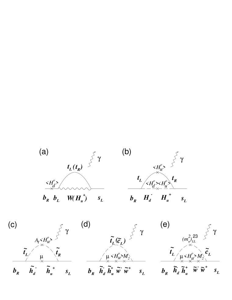
Figure 3: The most important diagrams for the $b\rightarrow s\gamma$ decay in the MSSM with large tan$\beta$, in the interaction basis. Note the enhancement of the chargino diagrams (c)–(e) by tan$\beta$ compared to the SM and charged Higgs diagrams (a) and (b).

For the Yukawa matrices, the exact equality of the 33 elements is assumed. The remaining Yukawa entries are, of course, dependent on specific properties of model 4c. However, they are small and decouple from the MSSM RGEs for the gauge and third generation Yukawa couplings, as well as for the diagonal SUSY mass parameters. Thus they have no effect on the calculation of the $Z$-scale values for the first nine observables in table 1. Only the branching ratio $BR(b\rightarrow s\gamma)$ is affected by some of these entries. This dependence comes dominantly from the diagram in figure 3e. The partial contribution to $b\rightarrow s\gamma$ is proportional to the flavor changing $\tilde{c}_{L}$-$\tilde{t}_{L}$ squark mixing in this case [23] and is tan$\beta$ enhanced which makes it non-negligable. The mixing is completely induced by the off-diagonal entries of the Yukawa matrices in the RG evolution, since we assume universal squark masses at the GUT scale. In addition, there is no significant pull in the model 4c best $\chi^{2}$’s from the light fermion masses and CKM mixing elements [5]. Instead, the dominant pulls are imposed by $\alpha_{s}(M_{Z})$, $m_{b}(M_{b})$ and other observables which also enter the MSSM analysis. Typically, about 60-80% of the total $\chi^{2}$ value comes from the first ten observables of table 1. That means that it is these traditional MSSM observables which drive the model 4c optimization procedure when it gets close to its minima and that at the same time the Yukawa sector of model 4c works indeed very well and does not bias the optimization significantly. We conclude that our results presented in this section are not sensitive to the structure of the Yukawa matrices except for the model dependent 23 mixing which is significant for the BR($b\rightarrow s\gamma$).

4.2 $BR({b\rightarrow s\gamma})$ in MSSM with large tan$\beta$

The SM, charged Higgs, and chargino diagrams contributing to the amplitude for $b\rightarrow s\gamma$ are shown in figures 3a–e. These are the dominant contributions in the best fits of our analysis. Note that the three chargino contributions in figures 3c–e are enhanced by tan$\beta$. In our code, we also take into account the gluino and neutralino diagrams as well as the full chargino contribution including the pieces not enhanced by tan$\beta$, although their contributions are numerically insignificant.

To understand our results which will be presented below, we would like to look first at an estimate what to expect from the SUSY contribution to $C_{7}(M_{Z})$. As a starting point we acknowledge the fact that the SM contribution gives a rough agreement with the measured rate and define the ratios for Higgs and chargino contributions

$$r^{(H)} = C_{7}^{(H)}\>/\>C_{7}^{(SM)}\>,$$ (5)

$$r^{(C)} = C_{7}^{(C)}\>/\>C_{7}^{(SM)}\>,$$ (6)

where all quantities are evaluated at $M_{Z}$. Equation (4) then reads

$$C_{7}^{(MSSM)\>eff}\approx\eta^{16\over 23}\>C_{7}^{(SM)}\,(1+r^{(H)}+r^{(C)})+\sum_{i=1}^{8}h_{i}\eta^{a_{i}}\,$$ (7)

where we used $C_{2}(M_{Z})=1$ and, for simplicity, neglected the mixing with the chromomagnetic operator, proportional to $C_{8}$, which turns out to be by about a factor 5–10 less than the other two terms.

Since $C_{7}^{(SM)\>eff}$ (approximately equal to $\eta^{16\over 23}\,C_{7}^{(SM)}+\sum h_{i}\eta^{a_{i}}\,$) would yield about the right value of the $BR(b\rightarrow s\gamma)$ we deduce that either

$$r^{(C)}\approx-r^{(H)}$$ (8)

for $C_{7}^{(MSSM)\>eff}\approx+C_{7}^{(SM)\>eff}$ , or

$$r^{(C)}\approx-r^{(H)}-4.60$$ (9)

for $C_{7}^{(MSSM)\>eff}\approx-C_{7}^{(SM)\>eff}$. For the last estimate, the numerical results $C_{7}^{(SM)}=-0.190$, $\eta^{16\over 23}=0.679$, and $\sum_{i=1}^{8}h_{i}\eta^{a_{i}}\,=-0.168$ were used — computed for $\alpha_{s}(M_{Z})=0.118$.

The charged Higgs contribution always interferes constructively with the SM contribution [7]. Typically, we get

$$0<r^{(H)}<1.3\,,$$ (10)

depending on the mass of the $H^{-}$. In the first case, especially if $r^{(H)}$ and $r^{(C)}$ are non-negligible, eq.(8) means that the chargino part must interfere destructively with the SM and charged Higgs contributions, practically cancelling the latter. The enhancement by tan$\beta$ of the chargino contribution has to be compensated for by rather large masses of the sparticles in the diagrams in figures 3c–e. In the second case, described by eq.(9), large destructive chargino interference is required to outweigh the combined SM and $H^{-}$ contributions and to flip the overall sign of the amplitude. Quite amazingly, it is not so difficult to arrange (see also [24]) since the chargino contribution is the only one enhanced by large tan$\beta$. However, large sparticle masses obviously suppress the effect. The lesson is that we can expect the two cases to work in a complementary SUSY parameter space and have sign$\,C_{7}^{(MSSM)}=\stackrel{{\scriptstyle+}}{{\scriptstyle(-)}}$ sign$\,C_{7}^{(SM)}$ for the best fits in the region with large (low) $m_{0}$ and/or $M_{1/2}$, respectively.

These expectations are indeed realized in the best fits of model 4c. Figure 2a shows the best fits in the case when the chargino contribution roughly cancels the charged Higgs contribution, while the best fits of figure 2b correspond to the case when the chargino piece truly dominates and reverses the sign of the overall amplitude. As anticipated, these two cases work in complementary regions of parameter space.

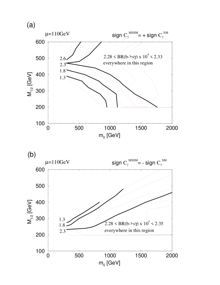
Figure 4: Contour lines of constant $BR(b\rightarrow s\gamma)\times 10^{4}$ in the best fits assuming the opposite signs of the effective amplitude for this process. For better reference, the $\chi^{2}$ contour plots of figures 2a and 2b are shown in the background of (a) and (b), respectively, as dotted lines.

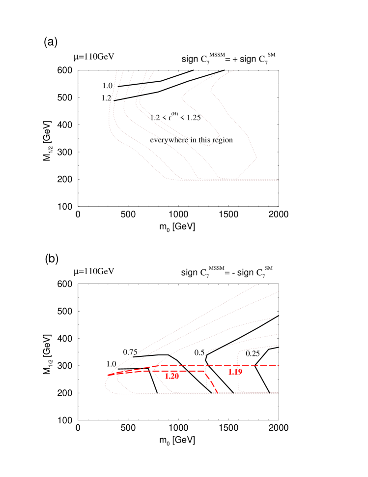
Figure 5: The same as in fig.4 for the contour plot of $r^{(H)}$ defined in eq.(5). The effect of the doubled minimum in the lower part of figure (b) corresponds to the possibility of having heavy (solid black curves) or light (dashed gray curves) Higgs spectrum for $M_{1/2}<300$GeV.

Figures 4a and 4b show how well the fits describe the measured value of the $BR(b\rightarrow s\gamma)$. In these figures (and similarly in the following ones) we show the contour lines of constant $\chi^{2}$ in the background for reference. As can be seen, the $BR(b\rightarrow s\gamma)$ indeed presents a major constraint since whenever the $\chi^{2}$ values go up, the agreement with the observed $b\rightarrow s\gamma$ decay rate gets worse. Figures 5a–b and 6a–b show the contour plots of constant $r^{(H)}$ and $r^{(C)}$ in each of these two cases. One can compare the numerical results in these figures with the approximate relations (8) and (9). Note also the validity of relation (10) in each case. Finally note that due to large tan$\beta$ the effects of SUSY decoupling start showing up only for $m_{0}>2$TeV, i.e. outside the SUSY space studied in these figures.

4.3 Discussion of the results for $BR({b\rightarrow s\gamma})$ and phenomenological implications

There is one striking feature which is common to both cases. It is that both fits would like to have the $BR(b\rightarrow s\gamma)$ below rather than above the current experimental value $2.32\times 10^{-4}$.

In the first case, the tan$\beta$ enhanced chargino contribution tends to be too large when going against the charged Higgs contribution, since the latter is not tan$\beta$ enhanced. The fit clearly favors as large Higgs contribution as possible with $r^{(H)}$ reaching its maximum (see fig.5a). A phenomenological consequence of this observation is that the charged Higgs (and then also the whole Higgs sector) tends to be as light as possible in this case. We get, for instance, the best fit value of the pseudoscalar mass $m_{A}<100$GeV everywhere in the $(m_{0},M_{1/2})$ plane.

In the second case, when the chargino part overshoots the combined SM and $H^{-}$ contributions we observe different effects in the regions with $M_{1/2}$ below and above (roughly) $300$GeV. For larger values of $M_{1/2}$ the chargino contribution clearly tends to be not big enough. As a result we might expect to see only very low values of $r^{(H)}$ in this region — complementary to the large values in fig.5a — and a very heavy Higgs sector. However, the best fit value of $r^{(H)}$ varies quite a bit indicating that the charged Higgs mass does not stay at some very large value. That is related to the observation [5] that one cannot have good fits with the Higgs sector much heavier than squarks. When $M_{1/2}$ gets below $300$GeV the $b\rightarrow s\gamma$ decay rate is no longer a strong constraint and two separate minima can be found in the course of the optimization. The two fits work equally well: $\chi^{2}$ in each case stays below 1 per 3dof. The minima differ by the best fit values of the Higgs masses: one minimum corresponds to $m_{h^{0}}$ and $m_{A}$ at the experimental lower limit (set to $65$GeV in our analysis) while these masses gradually rise in the second “valley” up to $700$GeV. When crossing the region with $M_{1/2}\approx 300$GeV towards larger $M_{1/2}$, the first “valley” vanishes and the optimization slides down to the second minimum because of the $BR(b\rightarrow s\gamma)$. In the allowed corner with $m_{0}<700$GeV, the two “valleys” approach each other and finally coincide. The effect of the doubled minima is indicated in figures 5b and 6b with the solid black (dashed gray) contour lines corresponding to the heavier (lighter) Higgs sector.

In summary, if the future experimental analysis confirms the discrepancy between the CLEO measured value and the NLO SM calculation [3], the MSSM with large tan$\beta$ could be the solution. Similarly, if the NLO calculation is completed for the MSSM, and if it turns out to increase the LO result as occurred for the SM, then the large tan$\beta$ regime will apparently have no problem fitting the $b\rightarrow s\gamma$ rate exactly. That seems to be in contrast with the fits in the low tan$\beta$ regime of ref.[9], which get below the SM value only for $M_{1/2}<200$GeV and small $m_{0}$.

4.4 Role of $\tilde{c}$-$\tilde{t}$ mixing in our results for $BR({b\rightarrow s\gamma})$

It is interesting to note the significance of the inter-generational squark mixing in fig.3e. In analogy to eq’s (5), (6) we define

$$r^{(C23)}=C_{7}^{(C23)}\>/\>C_{7}^{(SM)}\>,$$ (11)

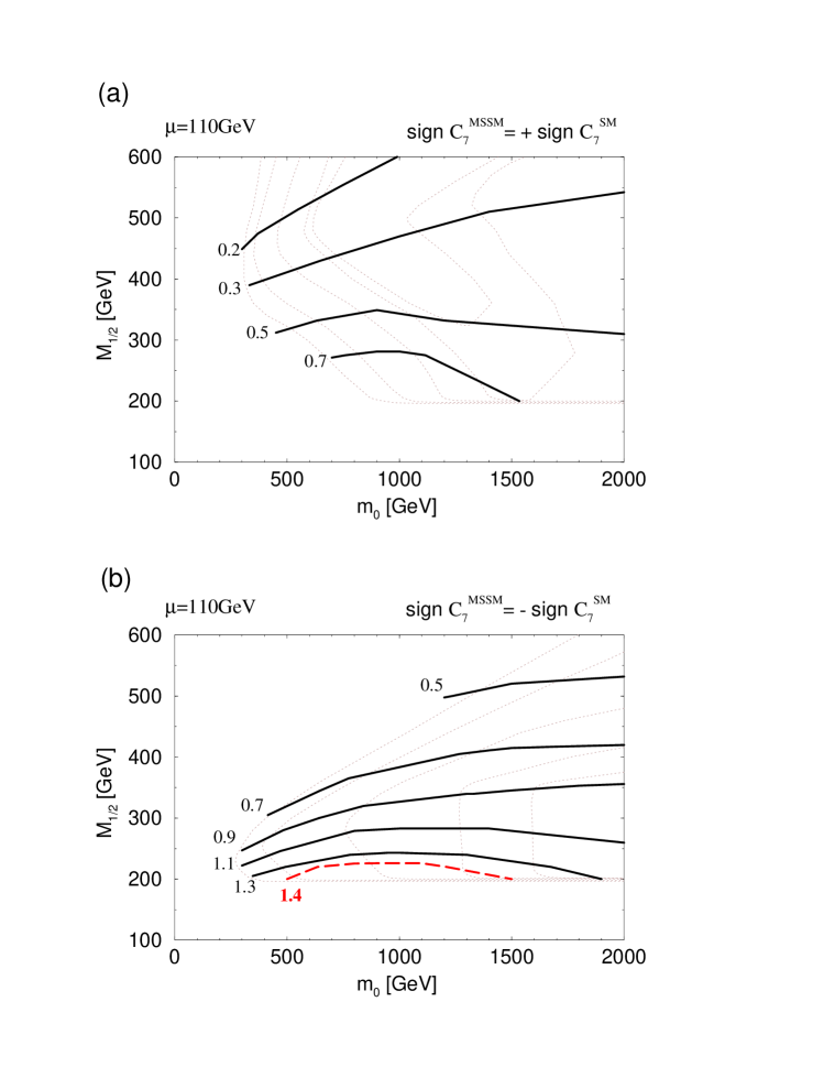
Figure 7: The same as in fig.5 for the contour plot of $r^{(C23)}$ defined in eq.(11).

where $C_{7}^{(C23)}$ is the $\tilde{c}_{L}$-$\tilde{t}_{L}$ mixing contribution to the coefficient $C_{7}$ at the scale $M_{Z}$. We show the contour plots of the constant $r^{(C23)}$ in figures 7a and 7b. While the dominant chargino contribution is that proportional to the $\tilde{t}_{L}$-$\tilde{t}_{R}$ mixing (fig.3c), $C_{7}^{(C23)}$ becomes important because of the destructive character of the interference among the partial amplitudes. As one can see, the $\tilde{c}_{L}$-$\tilde{t}_{L}$ mixing term can be comparable with the SM and $H^{-}$ contributions. More importantly, it always interferes constructively with them. In the case when sign$\,C_{7}^{(MSSM)}=+$ sign$\,C_{7}^{(SM)}$, this term helps to counterbalance the large contribution of the left-right stop mixing. In the complementary case, when the chargino contribution overturns the sign of the net amplitude the $\tilde{c}_{L}$-$\tilde{t}_{L}$ mixing makes this flip more difficult to happen. As a result, it has different consequences for the two fits in figures 2a and 2b, especially important in the region ($m_{0}\leq 1000$GeV,$\,M_{1/2}\approx 350$GeV) where the fits start getting worse. In figure 2a, it improves the fit for lower values of $(m_{0},M_{1/2})$ where the contribution from the stop mixing alone would otherwise overwhelm the sum of the SM and $H^{-}$ diagrams. On the contrary, it worsens the fit in figure 2b in the same parameter subspace. These observations are, however, model dependent as has been explained in the introduction to this section, and their validity relies on the boundary conditions assumed at the GUT scale. A general study of the limits imposed by the inter-generational mixings can be found in the review [23] and the references therein. To make a connection with the general approach we note that typically we get

$$(\delta^{23}_{U})_{LL}\equiv\frac{(m^{2}_{U})^{23}_{LL}}{[(m^{2}_{U})^{22}_{LL}(m^{2}_{U})^{33}_{LL}]^{1/2}}\sim-(0.01\mbox{-}0.02)\,$$ (12)

at the $Z$ scale, where $(m^{2}_{U})_{LL}$ is the $3\times 3$ $m^{2}_{Q}$ squark mass matrix after the unitary rotations which diagonalize the fermionic sector are performed in the squark sector too ( — sandwiching by $V_{U}^{L}$’s in this particular case). This value is to be compared with the flavor–changing effects originating in the CKM matrix (figures 3a–d) with $|V_{ts}|\approx|V_{cb}|\approx 0.04$.

4.5 Effects of NLO QCD Corrections to BR($b\rightarrow s\gamma$)

Finally, we would like to comment on the next-to-leading order (NLO) QCD corrections. These have been completed only for the SM [3]. In ref.[25] it was shown that the NLO matching at the high scale gives a non-negligible contribution to $C_{7}$. In particular, for the SM we get

$$C_{7}^{eff}(\mu_{b}) = C_{7}^{(0)\,eff}(\mu_{b})+\frac{\alpha_{s}}{4\pi}\,(\,\eta^{39/23}C_{7}^{(1)}(M_{Z})+\frac{8}{3}(\eta^{\frac{37}{23}}-\eta^{\frac{39}{23}})C_{8}^{(1)}(M_{Z})+\cdots)$$

$$= -0.312+0.017\,(-0.883-0.111+\cdots)\;,$$ (13)

where $C_{7}^{(0)\,eff}(\mu_{b})$ is given in terms of the LO matching coefficients (our eq.(4)) and for the evaluation in the second line $\alpha_{s}(M_{Z})=0.118$ was assumed. Hence within the SM the NLO matching corrections $C_{7}^{(1)}(M_{Z})$ and $C_{8}^{(1)}(M_{Z})$ alone would change the rate by about 10%. The final NLO corrected result increases the LO value obtained at $\mu_{b}\simeq M_{b}$ by about 20%. (In other words, it effectively lowers the scale $\mu_{b}$ of the LO calculations to about $0.6\,M_{b}$ as obtained also in ref.[9].) In the MSSM, the NLO matching remains to be calculated. Clearly, with large tan$\beta$ the chargino diagrams will likely dominate and their contribution may cause a different effect than in the SM. For that reason we have left our results without applying the NLO corrections and will just sketch at this point what effects the higher order matching corrections may have in our best fits.

The case when sign$\,C_{7}^{(MSSM)}=+$ sign$\,C_{7}^{(SM)}$ is much like the SM case. The effect of the unknown $C_{7}^{(MSSM)\,(1)}(M_{Z})$ and $C_{8}^{(MSSM)\,(1)}(M_{Z})$ can be readily estimated from the complete form of eq.(13) quoted in [3]. If the NLO matching followed the cancellation among the charged Higgs and chargino contributions observed in the LO (eq.(8)), our results for the $BR(b\rightarrow s\gamma)$ would also be about 20% larger, similar to the SM calculation. We can see from figure 4a that this would increase the parameter space in this case. Effectively, the NLO terms would add to the LO contributions of $W^{-}$ and $H^{-}$, enabling the tan$\beta$ enhanced chargino contribution to be greater in magnitude than what is allowed by eq.(8) — a welcome feature for lighter SUSY spectra. Clearly, if the NLO matching terms remain negative and get even larger in magnitude than in the SM case, the fit will improve substantially in the region with low $m_{0}$ and $M_{1/2}$ (and may get somehow worse in the upper left corner of the $(m_{0},M_{1/2})$ plane). On the other hand, we have checked that our LO results remain unaltered for $C_{k}^{(MSSM)\,(1)}\simeq-C_{k}^{(SM)\,(1)}$, $k=7,8$: for such matching terms all NLO corrections practically sum up to zero. Only if the NLO matching terms turn out to be very large and positive, the fit will be forced to retreat significantly towards larger $M_{1/2}$ values.

The second case, sign$\,C_{7}^{(MSSM)}=-$ sign$\,C_{7}^{(SM)}$, is obviously more sensitive to the unknown NLO matching. Despite the sensitivity our sample calculations indicate that a drop in the value of the $BR(b\rightarrow s\gamma)$ is fairly common and more likely to happen than an enhancement. For instance, we get $BR(b\rightarrow s\gamma)\times 10^{4}=0.98\,(2.31)$ in the complete NLO calculation assuming the NLO matching terms are $C_{k}^{(MSSM)\,(1)}=+1\,(-7)\times C_{k}^{(SM)\,(1)}$, $k=7,8$, and keeping $C_{7}^{(0)}$ and $C_{8}^{(0)}$ at the values which yield $BR(b\rightarrow s\gamma)\times 10^{4}=2.31$ at the LO. The reduction in the rate is correlated with the opposite signs of $C_{7}$ and $C_{8}$ as compared to the SM case. However, it still holds that the NLO correction would be effectively taken into account by lowering the scale in the LO calculation. For the region with $M_{1/2}>300$GeV, where the fit gradually gets worse in this case, it means that the $b\rightarrow s\gamma$ decay is likely more constraining than it appears in the analysis based on the LO calculation. As indicated above, the NLO corrections will improve the fit only if the NLO matching terms are at least seven times larger and opposite in sign compared to the SM NLO matching terms.

4.6 $\delta m_{b}^{SUSY}$, $\alpha_{s}(M_{Z})$ and $\epsilon_{3}$ in the Best Fits

For the presented results, it has been important to have a destructive interference among the partial contributions to $b\rightarrow s\gamma$. With the universal boundary conditions at the GUT scale however, that can be arranged only for a specific sign of the $\mu$ parameter: $\mu>0$ in our conventions. That in turn correlates with the positive sign of the SUSY corrections to the $b$ quark mass [26]. This fact implies strong constraints on the SUSY parameter space from $m_{b}$ since $\delta m_{b}^{SUSY}$ gets a dominant contribution from the tan$\beta$ enhanced gluino exchange, which tends to be very large [27] and offsets the agreement between the low energy value of $m_{b}$ and the $b$–$\tau$ unification at the GUT scale. The gluino correction can be explicitly suppressed by heavy squarks and by the chargino correction which enters with the opposite sign. It can also be reduced by lower values of $\alpha_{s}(M_{Z})$ because of the strong couplings in the vertices of the gluino – $b$-squark diagram. The contour plots of the total SUSY correction to $m_{b}(M_{Z})$ in the best fits are shown in figures 8a–b where one can see that these effects are quite effective in reducing the value of $\delta m_{b}$.

Note that the impact of large positive $\delta m_{b}^{SUSY}$ is reduced by a lower value of $\alpha_{s}(M_{Z})$ also indirectly — due to the RG evolution of the current $b$ mass from $M_{Z}$ down to $M_{b}$. The effect is enhanced if the current mass $m_{b}$ is converted to the perturbative pole mass $M_{b}$ in a top–down analysis. For example, the difference between $\alpha_{s}(M_{Z})$ being 0.115 and 0.121 leads to about 5% difference in $M_{b}$, if the same value of $m_{b}(M_{Z})$ is assumed in each case. This is a significant effect. In our analysis, which assumes larger uncertainty for $\alpha_{s}$ than for $m_{b}(M_{b})$, it pushes $\alpha_{s}(M_{Z})$ down. The effect can be seen in figures 9a–b. Note that one can trade lower values of $\alpha_{s}$ for higher values of $m_{b}$ provided a smaller uncertainty $\sigma(\alpha_{s})$ is assumed [28].

Rather low values of $\alpha_{s}(M_{Z})$ are, however, difficult to obtain from the exact gauge coupling unification, traditionally assumed in an MSSM analysis constrained by unification. In our analysis, we assumed that there is a few per cent correction to the gauge coupling unification generated by the spread in masses of heavy states integrated out at the GUT scale. It turned out that with a few per cent negative correction $\epsilon_{3}$ to $\alpha_{s}(M_{G})$ we can accommodate lower values of $\alpha_{s}(M_{Z})$ with no problem. The best fit values of $\epsilon_{3}$ are presented in figures 10a–b. Clearly, as squarks get lighter the SUSY correction to $m_{b}(M_{Z})$ (fig.8) has to be increasingly reduced by lower values of $\alpha_{s}(M_{Z})$ (fig.9), which in turn requires a more substantial departure from the gauge coupling unification (fig.10) in the respective SUSY parameter subspace.

5 Conclusions

In summary, we have presented the results of the MSSM analysis focusing on the constraint imposed by the measured value of the $BR(b\rightarrow s\gamma)$. The analysis was motivated by the best of the $SO(10)$ SUSY GUT models studied previously. Large tan$\beta$ was assumed as a consequence of simple SO(10) flavor dynamics. We showed that the effective amplitude for the inclusive $b\rightarrow s\gamma$ decay can be of either sign in such a scenario. In the case, when the sign is the same as in the SM calculation, the often neglected inter-generational $\tilde{c}_{L}$-$\tilde{t}_{L}$ squark mixing and the NLO correction tend to increase the allowed SUSY parameter space. The best fits favor light Higgs spectrum since a substantial charged Higgs contribution to $b\rightarrow s\gamma$ helps to counterbalance the chargino contribution. In the complementary case, when the sign of the $C_{7}$ coefficient is flipped by a large chargino contribution, both the $\tilde{c}_{L}$-$\tilde{t}_{L}$ mixing and the NLO correction work the other way and tend to reduce the allowed SUSY parameter space. The charged and pseudoscalar Higgs masses can be either large or small. In each case, the chargino (and neutralino) masses are at the experimental limit in the best fits. Because of $\delta m_{b}^{SUSY}>0$ the best fits result in rather low values of $\alpha_{s}(M_{Z})$, which can be obtained with a few per cent negative correction to $\alpha_{s}(M_{G})$. With these guidelines the large tan$\beta$ regime of the MSSM constrained by simple $SO(10)$ GUTs remains a viable option for physics beyond the Standard Model.

Acknowledgments

The authors would like to thank Marcela Carena and Carlos Wagner who collaborated on the early stages of this project. This research was supported in part by the U.S. Department of Energy under contract numbers DE-FG02-91ER40661 and DOE/ER/01545-729.

Figure 1: Contour lines of constant $\chi^{2}$ in the best fits of model 4c for $\mu(M_{Z})$ = ($a$) 80 GeV, ($b$) 160 GeV and ($c$) 240 GeV. Solid, dashed and dotted curves correspond to $\chi^{2}$= 6, 3 and 1 per 3 degrees of freedom, respectively.

Figure 2: $\chi^{2}$ contour plots in the best fits of model 4c with the MSSM effective amplitude for $b\rightarrow s\gamma$ of (a) the same (b) the opposite sign as compared to the SM amplitude. $\mu(M_{Z})$ = 110 GeV, which — as described in the text — basically corresponds to the minimum value if $\mu$ freely varied as an input parameter. As indicated, curves correspond to $\chi^{2}=6,\,3,\,1,\,0.4,\,0.3$ per $3\>d.o.f.$, respectively.

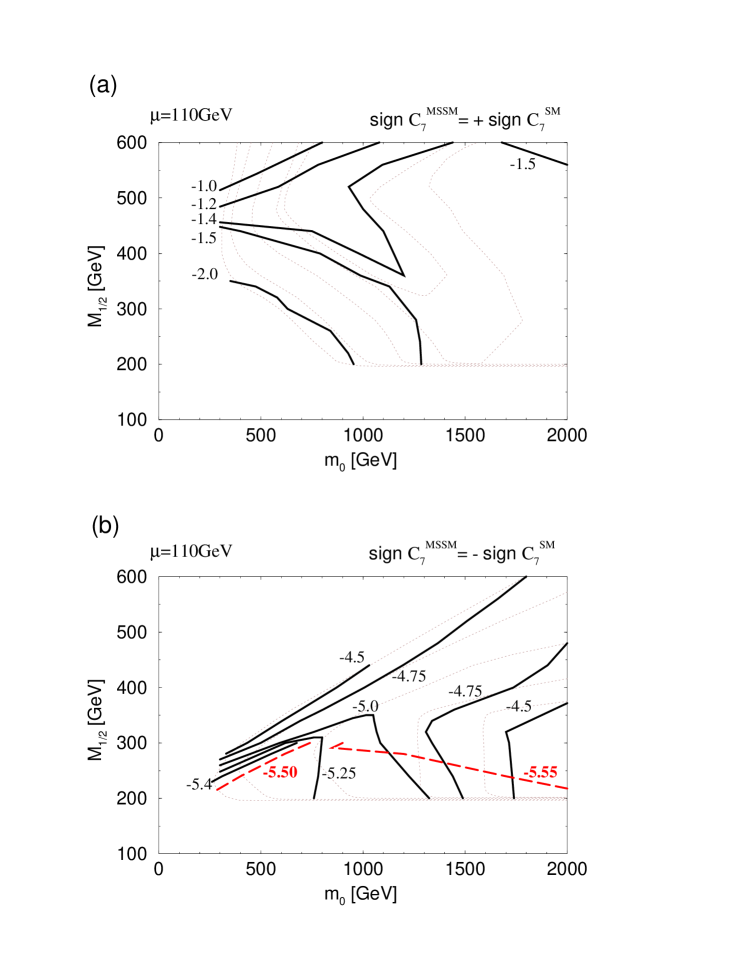
Figure 6: The same as in fig.5 for the contour plot of $r^{(C)}$ defined in eq.(6).

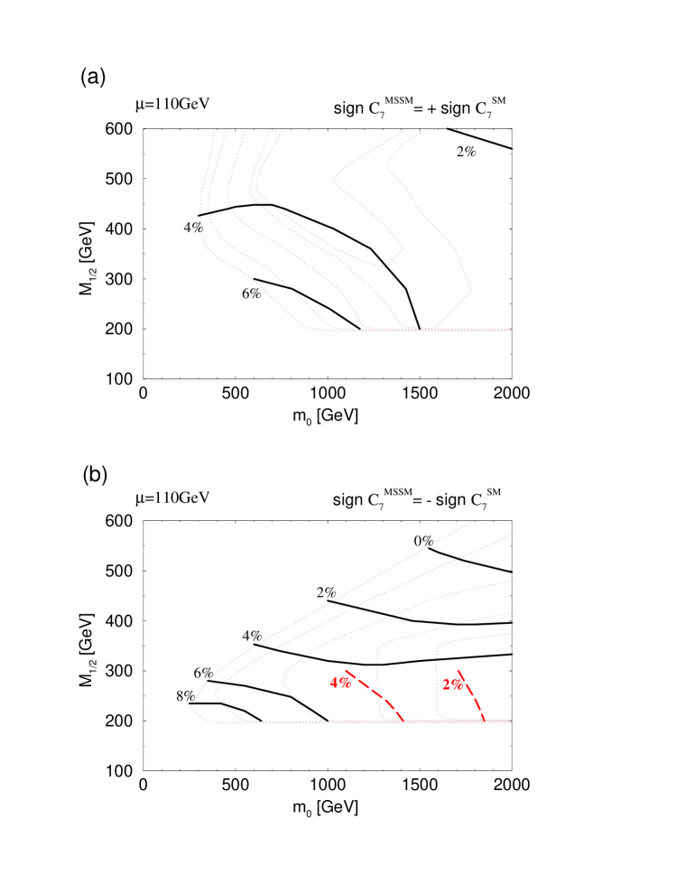
Figure 8: The same as in fig.5 for the contour plot of $\delta m_{b}^{SUSY}$, the SUSY correction to the $b$ quark mass $m_{b}(M_{Z})$.

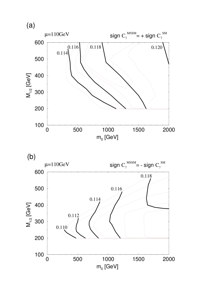
Figure 9: The same as in fig.4 for the contour plot of $\alpha_{s}(M_{Z})$.

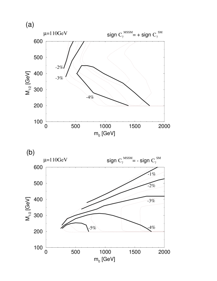
Figure 10: The same as in fig.4 for the contour plot of $\epsilon_{3}$, the GUT scale threshold correction to $\alpha_{s}$.

References

- [1] CLEO Collaboration, M.S. Alam et al., Phys.Rev.Lett. 74 (1995) 2885.
- [2] Aleph Coll., a preliminary result presented at the International Europhysics Conference on High Energy Physics, Jerusalem, Israel, August 19-26, 1997. To be published in the conference proceedings.
- [3] K. Chetyrkin, M. Misiak and M. Münz, hep-ph/9612313; A. Buras, A.J. Kwiatkowski and N. Pott, hep-ph/9707482; C. Greub and T. Hurth, hep-ph/9708214. The quoted SM value of the BR() is from Buras et al.
- [4] V. Lucas and S. Raby, Phys. Rev. D54, 2261 (1996).
- [5] T. Blažek, M. Carena, S. Raby and C.E.M. Wagner, Phys. Rev. D56 (1997) 6919.
-
[6]
S. Bertolini, F. Borzumati, A. Masiero and G. Ridolfi,
Nucl. Phys. B353 (1991) 591;
V. Barger, M.S. Berger, P. Ohmann and R.J.N. Phillips, Phys. Rev. D51 (1995) 2438;
H. Baer and M. Brhlik, Phys. Rev. D55 (1997) 3201. -
[7]
R. Barbieri and G.F. Giudice, Phys. Lett. B309 (1993) 86;
R. Garisto and J. Ng, Phys. Lett. B315 (1993) 372;
F. Borzumati, Z. Phys. C63 (1994) 291;
F. Borzumati, M. Olechowski and S. Pokorski, Phys. Lett. B349 (1995) 311;
D.M. Pierce and J. Erler, talk by D.M.P. at SUSY’97, Philadelphia, PE, May 1997, hep-ph/9708374;
J.L. Hewett and J.D. Wells, Phys. Rev. D55 (1997) 5549. - [8] W. de Boer, A. Dabelstein, W. Hollik, W. Moesle, U. Schwickerath, Z. Phys. C75 (1997) 627; for the update see [9].
- [9] W. de Boer, talk presented at the International Europhysics Conference on High Energy Physics, Jerusalem, Israel, August 19-26, 1997. To be published in the conference proceedings.
- [10] S. Martin and Vaughn, Phys. Rev. D50 (1994) 2282.
- [11] M.Carena, M.Quiros and C. Wagner, Nucl. Phys. B461 (1996) 407.
- [12] T. Blažek, S. Pokorski and S. Raby, Phys. Rev. D52 (1995) 4151.
- [13] D.M. Pierce, J. Bagger, K.T. Matchev and R. Zhang, Nucl. Phys. B491 (1997) 3.
- [14] P. Chankowski, Z. Pluciennik and S. Pokorski, Nucl. Phys. B439 (1995) 23.
-
[15]
O.V. Tarasov, A.A. Vladimirov and A.Y. Zharkov,
Phys. Lett. B93 (1980) 429;
S.G. Gorishny, A.L. Kataev and S.A. Larin, Sov. J. Nucl. Phys. 40 (1984) 329;
H. Arason, D.J. Castaño, B. Kesthelyi, S. Mikaelian, E.J. Piard, P. Ramond and B.D. Wright, Phys. Rev. D46 (1992) 3945;
V. Barger, M.S. Berger, and P. Ohmann, Phys. Rev. D47 (1993) 1093. - [16] P.Burrows, “Review of Measurements”, invited talk at the 3rd International Symposium on Radiative Corrections, Cracow, Poland, August 1 - 5, 1996. To be published in the conference proceedings.
- [17] Bertolini et al, in [6].
- [18] A.J. Buras, M. Misiak, M. Münz and S. Pokorski, Nucl. Phys. B424 (1994) 374.
- [19] Particle Data Group, Phys. Rev. D54 (1996) 1.
- [20] G. Anderson, S. Dimopoulos, L.J. Hall, S. Raby and G. Starkman, Phys. Rev. D49 (1994) 3660.
- [21] T. Blažek and S. Raby, Phys. Lett. B392 (1997) 371.
- [22] ALEPH Collaboration, “Preliminary ALEPH Results at 183 GeV”, presented at the International Europhysics Conference on High Energy Physics, Jerusalem, Israel, August 19-26, 1997. To be published in the conference proceedings.
- [23] M. Misiak, S. Pokorski and J. Rosiek, “Supersymmetry and FCNC Effects”, to appear in “Heavy Flavours II” (eds. A.J. Buras and M. Lindner, World Scientific, Singapore).
- [24] Garisto and Ng, in [7]
- [25] K.Adel and Y.P.Yao, Phys. Rev. D49 (1994) 4945.
- [26] M. Carena, M. Olechowski, S. Pokorski and C.E.M. Wagner, Nucl. Phys. B426 (1994) 269.
- [27] L.J. Hall, R. Rattazzi and U. Sarid, Phys. Rev. D50, (1994) 7048; R. Hempfling, Phys. Rev. D49, (1994) 6168.
- [28] T. Blažek and S. Raby, “Details of the study of the MSSM derived from a simple SO(10) SUSY GUTS”, in preparation.