IUHET-375 OHSTPY-HEP-T-97-022 November 1997

Global Analysis of Electroweak Data in SUSY GUTs 

Tomáš Blažek 
Department of Physics, Indiana University, Swain Hall West 117, Bloomington, IN 47405, USA and Stuart Raby 
Department of Physics, The Ohio State University, 174 W. 18th Ave., Columbus, OH 43210, USA

Abstract

A $\chi^{2}$ analysis of several SUSY GUTs recently discussed in the literature is presented. We obtain global fits to electroweak data, which include gauge couplings, gauge boson masses, $BR(b\rightarrow s\gamma)$ and masses of fermions of all three generations and their mixing angles. Thus we are able to test gauge unification, radiative electroweak symmetry breaking, SUSY sector ( – in the context of supergravity induced SUSY breaking) and the Yukawa sector in each particular model self-consistently. One of the models studied provides a very good fit with $\chi^{2}\sim 1$ for $3$ degrees of freedom, in a large region of the allowed SUSY parameter space. The Yukawa sector works so well in this case that the analysis ends up testing the MSSM constrained by unification. Adopting this point of view, in the second part of this talk we focus on the details of the fit for $BR(b\rightarrow s\gamma)$ and discuss the correlations among $\delta m_{b}^{SUSY}$, $\alpha_{s}(M_{Z})$ and a GUT threshold to $\alpha_{s}(M_{G})$. We conclude that an attractive $SO(10)$-derived regime of the MSSM remains a viable option.

A $\chi^{2}$ analysis of several SUSY GUTs recently discussed in the literature is presented. We obtain global fits to electroweak data, which include gauge couplings, gauge boson masses, $BR(b\rightarrow s\gamma)$ and masses of fermions of all three generations and their mixing angles. Thus we are able to test gauge unification, radiative electroweak symmetry breaking, SUSY sector ( – in the context of supergravity induced SUSY breaking) and the Yukawa sector in each particular model self-consistently. One of the models studied provides a very good fit with $\chi^{2}\sim 1$ for $3$ degrees of freedom, in a large region of the allowed SUSY parameter space. The Yukawa sector works so well in this case that the analysis ends up testing the MSSM constrained by unification. Adopting this point of view, in the second part of this talk we focus on the details of the fit for $BR(b\rightarrow s\gamma)$ and discuss the correlations among $\delta m_{b}^{SUSY}$, $\alpha_{s}(M_{Z})$ and a GUT threshold to $\alpha_{s}(M_{G})$. We conclude that an attractive $SO(10)$-derived regime of the MSSM remains a viable option.

1 Introduction

Reaching beyond the Minimal Supersymmetric Standard Model (MSSM) we apply global analysis to the search for grand unified theories (GUTs). That enables us to compare specific GUT models which become the MSSM as effective theory below the unification scale. In practice, it means that we test gauge unification, radiative electroweak symmetry breaking and the SUSY sector in the same way as the MSSM analysis constrained by unification $\!{}^{{\bf?}}$, but in addition we also test the Yukawa sector of the theory versus the observed fermion masses of all three generations and the Cabibbo-Kobayashi-Maskawa (CKM) matrix elements. Clearly, we agree with the MSSM analysis for models which describe the Yukawa sector very well.

There are plenty of models to be tested in this kind of analysis. For the beginning we start with models based on SO(10) gauge symmetry. SO(10) SUSY GUTs have been recognized as excellent candidates for an effective field theory below the Planck/string scale. They maintain the successful prediction for gauge coupling unification and provide a powerful and very economic framework for theories of fermion masses. This is because all the fermions of one generation are contained in the 16 dimensional representation of SO(10) - thus fermion mass matrices are related by symmetry. In the most predictive theories, the ratio of Higgs vevs - tan$\beta$ - is large, and the top quark is naturally heavy as found experimentally. However, as a consequence of large tan$\beta$ there are potentially large supersymmetric one-loop effects at the weak scale which could play an important role in fitting the fermion masses and mixings, and the FCNC processes like the observed $b\rightarrow s\gamma$ decay rate. Thus a self-consistent analysis becomes more powerful (and restrictive) than in a low tan$\beta$ scenario.

In sections 3 and 4, we present the results of such a complete top-down analysis. In section 5, we focus on the MSSM constrained by the best working GUT model and analyze it similarly to generic MSSM analyses constrained by unification. We present the best fit correlations among various contributions to the $b\rightarrow s\gamma$ decay rate, SUSY corrections to $m_{b}$, and rather low values of $\alpha_{s}(M_{Z})$ – all in the $(m_{0},M_{1/2})$ SUSY parameter space. The phenomenological implications are discussed as well.

2 Global Analysis

Details of our numerical procedure are described in $\!{}^{{\bf?}}$. The analysis starts at the GUT scale $M_{G}$, which is a free parameter itself, with unified gauge coupling $\alpha_{G}$, $n_{y}$ free parameters entering the Yukawa matrices, and with $\epsilon_{3}$ as a one loop GUT threshold correction to $\alpha_{s}(M_{G})$ . We assume supergravity induced SUSY breaking. At the scale $M_{G}$ we introduce standard universal soft SUSY breaking parameters $m_{0},\>M_{1/2}$ and $A_{0}$, and non-universal Higgs masses $m_{H_{d}}$ and $m_{H_{u}}$. The $\mu$ parameter and its SUSY breaking bilinear partner $B$ are introduced at the $Z$ scale, since they are renormalized multiplicatively and do not enter the RGEs of the other parameters. At the $Z$ scale we match the MSSM directly to $SU(3)_{c}\times U(1)_{em}$, thus leaving out the SM as an effective theory $\!{}^{{\bf?}}$. Electroweak symmetry breaking is established at one loop in the process of the $\chi^{2}$ minimization by fitting the observables in table 1. Within the MSSM, we calculate one-loop corrected $W$ and $Z$ masses and $G_{\mu}$, corrections to the $\rho$ parameter from new physics outside the SM, and the amplitude for the process $b\rightarrow s\gamma$. When crossing the $Z$ scale, we compute the complete one loop threshold corrections to $\alpha_{s}$ and $\alpha$, whereas only those one loop threshold corrections to the fermion masses and mixings enhanced by tan$\beta$ are computed $\!{}^{{\bf?}}$.

Table 1: Experimental observables of the global analysis.

$$\begin{array}[]{|r|c|c|c||r|c|c|c|}\hline\cr\vrule\lx@intercol\hfil\rm Observable\hfil\lx@intercol\vrule\lx@intercol&{\rm Central}&\sigma&\lx@intercol\hfil\rm Observable\hfil\lx@intercol\vrule\lx@intercol&{\rm Central}&\sigma\\ \vrule\lx@intercol\hfil\hfil\lx@intercol\vrule\lx@intercol&\makebox[48.36958pt]{\rm value}&\makebox[48.36958pt]{}&\lx@intercol\hfil\hfil\lx@intercol\vrule\lx@intercol&\makebox[48.36958pt]{\rm value}&\makebox[48.36958pt]{}\\ \hline\cr 1.&M_{Z}&91.186&\underline{0.46}&11.&M_{b}-M_{c}&3.4&0.2\\ 2.&M_{W}&80.356&\underline{0.40}&12.&m_{s}&180&50\\ 3.&G_{\mu}&1.166\cdot 10^{-5}&\underline{1.2\cdot 10^{-7}}&13.&m_{d}/m_{s}&0.05&0.015\\ 4.&\alpha^{-1}&137.04&\underline{0.69}&14.&Q^{-2}&0.00203&0.00020\\ 5.&\alpha_{s}(M_{Z})&0.118&0.005&15.&M_{\mu}&105.66&\underline{0.53}\\ \cline{1-4}\cr 6.&M_{t}&175.0&6.0&16.&M_{e}&0.5110&\underline{0.0026}\\ \cline{5-8}\cr 7.&m_{b}(M_{b})&4.26&0.11&17.&V_{us}&0.2205&0.0026\\ 8.&M_{\tau}&1.777&\underline{0.0089}&18.&V_{cb}&0.0392&0.003\\ \cline{1-4}\cr 9.&\rho_{new}&-0.6\cdot 10^{-3}&2.6\cdot 10^{-3}&19.&V_{ub}/V_{cb}&0.08&0.02\\ 10.&B(b\rightarrow s\gamma)&2.32\cdot 10^{-4}&0.92\cdot 10^{-4}&20.&\hat{B}_{K}&0.8&0.1\\ \hline\cr\end{array}$$

The $Z$-scale amplitude for $b\rightarrow s\gamma$ is matched to the coefficient $C_{7}(M_{Z})$ which is then renormalized down to the scale $M_{b}$,

$$C_{7}^{eff}(M_{b})=\eta^{16\over 23}C_{7}(M_{Z})+{8\over 3}\>(\eta^{14\over 23}-\eta^{16\over 23})\>C_{8}(M_{Z})+C_{2}(M_{Z})\,\sum_{i=1}^{8}h_{i}\eta^{a_{i}}\,,$$ (1)

based on mixing of the electromagnetic operator with the chromomagnetic and current-current operators (coefficients $C_{8}$ and $C_{2}$) in the leading log approximation; with $\eta=\alpha_{s}(M_{Z})/\alpha_{s}(M_{b})$. Finally, the branching ratio

$$BR(b\rightarrow s\gamma)=\frac{|V^{*}_{ts}V_{tb}|^{2}}{|V_{cb}|^{2}}\;\frac{6\alpha}{\pi g(M_{c}/M_{b})}\;|C_{7}^{eff}(\mu_{b})|^{2}\;BR(b\rightarrow ce\bar{\nu})\;,$$ (2)

where $BR(b\rightarrow ce\bar{\nu})=0.104$, $\alpha=1/132.5$, the phase-space function $g(z)=1-8z^{2}+8z^{6}-z^{8}-24z^{4}\log z$, and $h_{i}$’s and $a_{i}$’s in eq.(1) are given in ref.$\!{}^{{\bf?}}$. The values of the CKM matrix elements and quark masses in (2) are consistently calculated in the actual fit within a particular model.

Note that $M_{Z},\>M_{W},\>\alpha,\>G_{\mu}$ and the lepton masses are known so well that we have to assign a theoretical error as their standard deviation ( — the corresponding $\sigma$’s are underlined in table 1). We estimated conservatively the theoretical error to be 0.5% based on the uncertainties from higher order perturbation theory and from the performance of our numerical analysis. The error on $G_{\mu}$ is estimated to be within 1% due to the fact that in addition to the uncertainties mentioned above we neglect SUSY vertex and box corrections to $\Delta r$. Also note that $\epsilon_{K}$, the observable of $CP$ violation, has been replaced by a less precisely known hadronic matrix element $\hat{B}_{K}$ . Similarly, the light quark masses are replaced by their ratios (at the scale 1GeV), and $m_{c}(M_{c})$ by the difference $M_{b}-M_{c}$, since the latter quantities are known to better accuracy. $Q^{-2}\doteq(m_{d}^{2}-m_{u}^{2})/m_{s}^{2}$ is the Kaplan-Manohar-Leutwyler ellipse parameter. Finally note, that the data in table 1 are divided into two groups. The first ten, i.e. five observables in the gauge sector ($M_{Z},\,M_{W},\,G_{\mu},\,\alpha$ and $\alpha_{s}$), masses of the third generation fermions, $\rho_{new}$ and $BR(b\rightarrow s\gamma)$ can also be included in tests of the MSSM constrained by unification with no particular underlying GUT. The other ten correspond to six light fermion masses and four independent parameters of the CKM matrix and test primarily the Yukawa sector of a GUT model.

In addition, the $\chi^{2}$ function is increased significantly by a special penalty whenever a sparticle mass goes below its experimental limit.

3 Results for SO(10) GUT Models with Four Effective Operators

The analysis, as described above, was used to test simple SO(10) models. First we checked the performance of the nine models with four effective operators suggested in $\!{}^{{\bf?}}$. The models were defined by a unique choice of the operators ${{\cal O}_{33}}=16_{3}\>10\>16_{3}$ and ${{\cal O}_{12}}=16_{1}\>(\frac{\tilde{A}}{S})^{3}\>10\>(\frac{\tilde{A}}{S})^{3}\>16_{2}$ at the GUT scale ($A$’s stand for adjoint states and $S$ for singlets). There were six ${\cal O}_{22}$ operators which all gave the same 0:1:3 Clebsch relation between the $22$ elements of the Yukawa matrices for the up quarks, down quarks and charged leptons, thus introducing Georgi-Jarlskog relation in all models. Finally, the models were distinguished by a choice of the ${\cal O}_{23}$ operator. Nine operators were suggested in ref.$\!{}^{{\bf?}}$ leading to different predictions at low energies.

Our analysis has shown that the choice of the ${\cal O}_{23}$ operator is indeed significant (see fig.1a) and that model 4 is by far the best working model. In this case, ${{\cal O}_{23}}=16_{2}\>(\frac{A_{2}}{\tilde{A}})\>10\>(\frac{A_{1}}{\tilde{A}})\>16_{3}$. Note that with four effective operators we have $n_{y}=5$ free parameters in the Yukawa matrices at the GUT scale. That leaves the $\chi^{2}$ function (out of the 20 observables in table 1) with 5 degrees of freedom (d.o.f.). We show in fig.1b that the performance of model 4 does not get significantly better in a larger SUSY parameter space. We checked that the same is true for the other models. We also checked that no substantial improvement of the performance of model 4 can be achieved by neglecting one out of the twenty observables given in table 1 $\!{}^{{\bf?}}$. On the other hand, we have found that a significant improvement is possible by adding one new operator, contributing to the 13 and 31 elements of the Yukawa matrices.

4 Results for SO(10) GUT Models with Five Effective Operators

Next, we analyzed two models recently derived from the complete SO(10) SUSY GUTs $\!{}^{{\bf?}}$. The models were constructed

Figure 1: Results of global analysis for SO(10) GUT models: (a) nine models of section 3; (b) model 4 [solid (dashed, short-long-dashed, dotted) lines represent contour lines of constant $\chi^{2}=16\,(15,\,14,\,13)$ per 5 d.o.f.]; (c) model 4c [solid (dashed, dotted) lines represent contour lines of constant $\chi^{2}=6\,(3,\,1)$ per 3 d.o.f.].

as simple extensions of model 4. Different label (a,b,…f) refers to the different possible 22 operators. In the extension to a complete GUT the different 22 operators lead to inequivalent theories due to different U(1) charge assignments. When one demands “naturalness”, i.e. includes all terms in the superpotential consistent with the symmetries of the theory one finds one and only one 13 operator for models 4a and 4c. The 22 and 13 operators of model 4c are ${{\cal O}_{22}}=16_{2}\>{\tilde{A}\over S}\>10\>{A_{1}\over S}\>16_{2}$ and ${{\cal O}_{13}}=16_{1}\>({\tilde{A}\over S})^{3}\>10\>{A_{2}\over S}\>16_{3}\;\;$. With the 13 operator $n_{y}$=7, which implies 3 degrees of freedom. The results of the global analysis are given in fig.1c. Similarly to fig.1b, these figures show the contour plots of the minimum $\chi^{2}$ in the $(m_{0},M_{1/2})$ plane, for three different fixed values of the parameter $\mu(M_{Z})=80,\,160,\,240$ GeV. All initial parameters other than {$m_{0},M_{1/2},\mu$} were subject to minimization.

The fits get worse as $\mu$ increases because the SUSY corrections to fermion masses and mixings increase with $\mu$. As $\mu$ gets larger they can only be kept under control by larger squark masses. Varying $\mu$ freely actually results in its approaching the lowest possible value. The lower bound on $\mu(M_{Z})$ is determined by the chargino mass limit from direct searches and is correlated with $M_{1/2}$. When the value of $\mu$ is fixed, as in fig’s 1b-c, the chargino mass limit then sets a sharp lower bound on $M_{1/2}$, which is explicitly visible in each of the figures. Figures 1b and 1c were obtained assuming $m_{\chi^{-}}>65$GeV. In our further analysis $\mu(M_{Z})$ has been fixed to $110$GeV and $m_{\chi^{-}}>85$GeV was imposed. Figures 2a-b show explicitly that the structure observed in fig.1c originates from the two distinct fits corresponding to two separate minima of the global analysis. The fits are primarily distinguished by the sign of the $b\rightarrow s\gamma$ decay amplitude. ( See section 5 for more details.) We do not show the results for negative values of $\mu$. In this case, the chargino contribution to $b\rightarrow s\gamma$ interferes constructively with the already large enough SM and charged Higgs contributions. As a result, the fits get much worse, with $\chi^{2}$ well above 10 per 3 d.o.f., and that disfavors this region of the SUSY parameter space. Similar observations were also made by W. Hollik et al $\!{}^{{\bf?}}$.

Model 4a is defined by different 22 and 13 operators and gives the fits with the best $\chi^{2}\simeq$4-6 in most of the parameter space. (It yields also $\chi^{2}\simeq$3, but only for the corner in the SUSY parameter space with large $m_{0},\>M_{1/2}$ and $\mu$.) $\!{}^{{\bf?}}$

Whether or not these particular models are close to the path Nature has chosen remains to be seen. One important test will be via the CP violating decays of the B meson. Models 4c and 4a both predict a narrowly spread value sin2$\alpha\simeq 0.95$, whereas in the SM the value of sin2$\alpha$ is unrestricted $\!{}^{{\bf?}}$. Another important test may come from nucleon decay rates $\!{}^{{\bf?}}$.

5 MSSM Analysis Constrained by the Best Working GUT Model

Since the fermionic sector of model 4c works very well, we can regard the analysis in this case as a test of the MSSM with large tan$\beta$. Yet, some model dependence is still present. It is, first of all, the introduction of $\epsilon_{3}$, a GUT threshold to $\alpha_{s}$. It is actually the only GUT threshold introduced in our study. Note in subsection 5.3 that non-zero $\epsilon_{3}$ is imposed by the low energy phenomenology rather than by physics at the GUT scale.

For the Yukawa matrices, the exact equality of the 33 elements is assumed. The remaining Yukawa entries are small and decouple from the MSSM RGEs for the gauge and third generation Yukawa couplings and diagonal SUSY mass parameters. Thus they have no effect on the calculation of the $Z$-scale values for the first nine observables in table 1. The $BR(b\rightarrow s\gamma)$ is affected by some of these entries. Model dependence comes from the chargino contribution which contains inter-generational $\tilde{c}_{L}$-$\tilde{t}_{L}$ squark mixing. That contribution is tan$\beta$ enhanced which makes it non-negligible. The mixing is completely induced by the off-diagonal entries of the Yukawa matrices in the RG evolution. Next, note that the light quark and lepton masses and CKM elements do not exert any significant pull on the best $\chi^{2}$’s of model 4c $\!{}^{{\bf?}}$. We conclude that our results presented in this section are not sensitive to the structure of the Yukawa matrices except for the model dependent 23 mixing which is significant for the $BR(b\rightarrow s\gamma)$.

5.1 Results for $BR({b\rightarrow s\gamma})$

We find that the $b\rightarrow s\gamma$ amplitude is dominated by the SM, charged Higgs, and tan$\beta$ enhanced chargino contributions. To understand our results, let’s estimate first what to expect from the SUSY contribution to $C_{7}(M_{Z})$ and define the $Z$ scale ratios for Higgs and chargino contributions $r^{(H)}=C_{7}^{(H)}/C_{7}^{(SM)}$ and $r^{(C)}=C_{7}^{(C)}/C_{7}^{(SM)}$. Equation (1) then reads

$$C_{7}^{(MSSM)\>eff}\approx\eta^{16\over 23}\>C_{7}^{(SM)}\,(1+r^{(H)}+r^{(C)})+\sum_{i=1}^{8}h_{i}\eta^{a_{i}}\,$$ (3)

where we used $C_{2}(M_{Z})=1$ and $C_{8}\ll C_{7},\,C_{2}$. Since it is well known that $C_{7}^{(SM)\>eff}\>(\approx\eta^{16\over 23}\,C_{7}^{(SM)}+\sum_{i=1}^{8}h_{i}\eta^{a_{i}})$ would yield about the right value for the $BR(b\rightarrow s\gamma)$ we infer that either

$$r^{(C)} \approx -r^{(H)}\,,\>\>\>\>\>\>\>\>\>\>\>\>\>\>\>\>\mbox{\rm for}\>C_{7}^{(MSSM)\>eff}\approx+\,C_{7}^{(SM)\>eff}\,,$$ (4)

or

$$r^{(C)} \approx -r^{(H)}-4.60\,,\>\>\>\mbox{\rm for}\>C_{7}^{(MSSM)\>eff}\approx-\,C_{7}^{(SM)\>eff}.$$ (5)

For the last estimate, the numerical results $C_{7}^{(SM)}=-0.190$, $\eta^{16\over 23}=0.679$, and $\sum_{i=1}^{8}h_{i}\eta^{a_{i}}\,=-0.168$ were used — computed for $\alpha_{s}(M_{Z})=0.118$.

The charged Higgs contribution always interferes constructively with the SM contribution. We get $0<r^{(H)}<1.3$, depending on the mass of the $H^{-}$. In the first case, especially if $r^{(H)}$ and $r^{(C)}$ are non-negligible, eq.(4) means that the chargino part must interfere destructively with the SM and charged Higgs contributions, practically cancelling the latter. The enhancement by tan$\beta$ of the chargino contribution has to be compensated for by rather large sparticle masses. In the second case, described by eq.(5), large destructive chargino interference is required to outweigh the combined SM and $H^{-}$ contributions and to flip over the overall sign of the amplitude. Quite amazingly, it is not so difficult to arrange since the chargino contribution is the only one enhanced by large tan$\beta$. However, large sparticle masses obviously suppress the effect. The lesson is that we can expect the two cases to work in a complementary SUSY parameter space and have sign$\,C_{7}^{(MSSM)}=\stackrel{{\scriptstyle+}}{{\scriptstyle(-)}}$ sign$\,C_{7}^{(SM)}$ for the best fits in the region with large (low) $m_{0}$ and/or $M_{1/2}$, respectively.

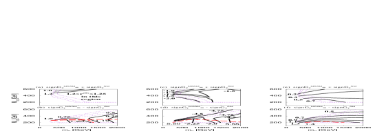
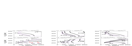
Figure 2: Model 4c global analysis results for the two possible signs of $C_{7}^{MSSM}$. The best fit contour plots of (a),(b) $\chi^{2}$ [solid (dashed, dotted) lines correspond to $\chi^{2}=6\,(3,\,1)$ per 3 d.o.f.]; (c),(d) BR$(b\rightarrow s\gamma)\times 10^{4}$ ; (e),(f) the lightest stop mass $m_{\tilde{t}_{1}}$ [in GeV]; with the $\chi^{2}$ contour lines in the background.

Figure 3: Relative contributions to $C_{7}$ for the two possible signs of $C_{7}^{MSSM}$. Contour plots of (a),(b) $r^{(H)}$; (c),(d) $r^{(C)}$; (e),(f) $r^{(C23)}$; with the $\chi^{2}$ contour lines in the background.

Figure 4: Contour plots of (a),(b) $\delta m_{b}^{SUSY}$; (c),(d) $\alpha_{s}(M_{Z})$; (e),(f) GUT threshold $\epsilon_{3}$; with the $\chi^{2}$ contour lines in the background.

These expectations are indeed realized in the best fits of model 4c. Figure 2a (2b) corresponds to the case when the $b\rightarrow s\gamma$ amplitude in MSSM is of the same (opposite) sign as the SM amplitude. As anticipated, these two cases work in complementary regions of parameter space. Figures 2c-d show how well the fits describe the measured value of the $BR(b\rightarrow s\gamma)$. In these figures (and similarly in the following ones) we show the $\chi^{2}$ contour lines of fig’s 2a-b in the background for reference. As can be seen, the $BR(b\rightarrow s\gamma)$ presents a major constraint since whenever the $\chi^{2}$ values go up, the agreement with the observed $b\rightarrow s\gamma$ decay rate gets worse. For the flipped sign of the amplitude it is interesting that the lightest stop $\tilde{t}_{1}$ can be sufficiently light (see fig.2f) to maintain the required large size of the chargino contribution even for $m_{0}$ at $2$TeV. That can be arranged due to significant left-right stop mixing and the freedom in varying the trilinear scalar coupling $A_{0}(M_{G})$. The corresponding $\tilde{t}_{L}$-$\tilde{t}_{R}$ mixing angle changes between 31^o to 40^o across the $(m_{0},M_{1/2})$ plane while the trilinear coupling $A_{t}(M_{Z})$ ranges from $-300$ to $-1700$GeV in this case. Figure 3 shows the contour plots of constant $r^{(H)}$ and $r^{(C)}$ for different signs of $C_{7}^{MSSM}$. One can compare the numerical results in figures 3a vs. 3c and 3b vs. 3d with the approximate relations (4) and (5).

There is one striking feature which is common to both cases. It is that both fits would like to have the $BR(b\rightarrow s\gamma)$ below rather than above the CLEO experimental value $2.32\times 10^{-4}$. $\!{}^{{\bf?}}$

In the first case, the tan$\beta$ enhanced chargino contribution tends to be too large when going against the charged Higgs contribution, since the latter is not tan$\beta$ enhanced. The fit clearly tries to make the Higgs contribution as large as possible (see fig.3a). As a result, the charged Higgs (and then also the whole Higgs sector) tends to be light. We get, for instance, the best fit value of the pseudoscalar mass $m_{A}<100$GeV everywhere in the $(m_{0},M_{1/2})$ plane.

In the second case, when the sign of $C_{7}$ is flipped by the chargino contribution, this contribution tends to be not big enough, especially if $M_{1/2}>300$GeV. Hence $b\rightarrow s\gamma$ would prefer a heavy charged Higgs. However, one cannot have good fits with the Higgs sector much heavier than squarks $\!{}^{{\bf?}}$ and thus $r^{(H)}$ varies quite a bit across the SUSY parameter space (see fig.3b). When $M_{1/2}$ gets below $300$GeV, $b\rightarrow s\gamma$ is no longer a strong constraint and two separate minima can be found in the course of optimization. The two fits work equally well ($\chi^{2}$ in each case stays below 1 per 3 d.o.f.) and differ only by the best fit values of the Higgs masses. One minimum corresponds to $m_{h^{0}}$ and $m_{A}$ settled at the experimental lower limit ($65$GeV, in our analysis) while these masses gradually rise up to $700$GeV in the second “valley”. In the allowed corner with $m_{0}<700$GeV, the two “valleys” approach each other and eventually coincide. The effect of the doubled minimum is indicated in figures 3b, 3d, 3f and 4b with the solid black (dashed gray) contour lines corresponding to the heavier (lighter) Higgs sector.

Can the NLO QCD corrections to BR($b\rightarrow s\gamma$) improve the fits? The calculation of these corrections has not been completed in the MSSM. Here we just summarize$\!{}^{{\bf?}}$ that the rate goes up if the unknown MSSM matching corrections satisfy $C_{k}^{(MSSM)\,(1)}/\,C_{k}^{(SM)\,(1)}\stackrel{{\scriptstyle>}}{{\sim}}-1$, ($k=7,8$), in the case when sign$\,C_{7}^{(MSSM)}=+$ sign$\,C_{7}^{(SM)}$. Thus the allowed SUSY parameter space is likely to increase in this case. In the second case, with the opposite sign of the $b\rightarrow s\gamma$ amplitude, the NLO correction will more likely make the fit worse. In this case, the net NLO correction increases the rate only if $C_{k}^{(MSSM)\,(1)}/C_{k}^{(SM)\,(1)}\stackrel{{\scriptstyle<}}{{\sim}}-7$, $k=7,8$.

In summary, if the future experimental analysis confirms the discrepancy between the CLEO measured value and the NLO SM calculation $\!{}^{{\bf?}}$, the MSSM with large tan$\beta$ could be the solution. Similarly, if the NLO calculation is completed for the MSSM, and if it turns out to enhance the LO result as occurred for the SM, then the large tan$\beta$ regime will apparently have no problem fitting the $b\rightarrow s\gamma$ rate exactly.

5.2 Role of $\tilde{c}$-$\tilde{t}$ mixing for $BR({b\rightarrow s\gamma})$

In analogy to previously defined $r^{(H)}$ and $r^{(C)}$ we introduce $r^{(C23)}\!=C_{7}^{(C23)}\,/\>C_{7}^{(SM)}$, where $C_{7}^{(C23)}$ is the $\tilde{c}_{L}$-$\tilde{t}_{L}$ mixing contribution to the coefficient $C_{7}$ at the scale $M_{Z}$. We show the contour plots of the constant $r^{(C23)}$ in fig’s 3e-f. While the dominant chargino contribution is that proportional to the $\tilde{t}_{L}$-$\tilde{t}_{R}$ mixing, $C_{7}^{(C23)}$ becomes important because of the destructive character of the interference among the partial amplitudes. As one can see, the $\tilde{c}_{L}$-$\tilde{t}_{L}$ mixing term can be comparable with the SM and $H^{-}$ contributions. More importantly, it always interferes constructively with them. In the case when sign$\,C_{7}^{(MSSM)}=+$ sign$\,C_{7}^{(SM)}$, this term helps to counterbalance the large contribution of the left-right stop mixing. In the complementary case, when the chargino contribution flips the sign of the net amplitude the $\tilde{c}_{L}$-$\tilde{t}_{L}$ mixing makes it more difficult to happen. As a result, it has different consequences for the two fits in figures 2a and 2b, especially important in the region ($m_{0}\leq 1000$GeV,$\,M_{1/2}\approx 350$GeV) where the fits start getting worse. These observations are, however, model dependent and their validity relies on the boundary conditions assumed at the GUT scale.

5.3 Correlations among $\epsilon_{3}$, $\alpha_{s}(M_{Z})$ and $\delta m_{b}^{SUSY}$

The results on $b\rightarrow s\gamma$ show that it is important to have a destructive interference among the partial contributions to $b\rightarrow s\gamma$. However, with the universal boundary conditions at the GUT scale that can be arranged only for a specific sign of the $\mu$ parameter: $\mu>0$ in our conventions. That in turn correlates with the positive sign of the SUSY corrections to the $b$ quark mass. This fact implies strong constraints on the SUSY parameter space from $m_{b}$ since $\delta m_{b}^{SUSY}$ gets a dominant contribution from the tan$\beta$ enhanced gluino exchange. The gluino correction can be explicitely suppressed by heavy squarks and by the chargino correction which enters with the opposite sign. It can also be reduced by lower values of $\alpha_{s}(M_{Z})$ because of the strong coupling in the vertices of the gluino – $b$-squark diagram. The contour plots of the net SUSY correction to $m_{b}(M_{Z})$ in the best fits are shown in figures 4a-b where one can see that these effects are quite effective in reducing $\delta m_{b}^{SUSY}$.

Note that the effect of large positive $\delta m_{b}^{SUSY}$ is also reduced by a lower value of $\alpha_{s}(M_{Z})$ indirectly — due to the RG evolution of the current $b$ mass from $M_{Z}$ down to $M_{b}$. In our analysis, which assumes larger uncertainty for $\alpha_{s}$ than for $m_{b}(M_{b})$, it pushes $\alpha_{s}(M_{Z})$ down (see figures 4c-d). One can trade lower values of $\alpha_{s}$ for higher values of $m_{b}$ provided a smaller uncertainty $\sigma(\alpha_{s})$ is assumed. Rather low values of $\alpha_{s}(M_{Z})$ are, however, difficult to obtain from an exact gauge coupling unification. Our analysis shows that a few per cent negative correction to $\alpha_{s}(M_{G})$ is enough to get $\alpha_{s}(M_{Z})\stackrel{{\scriptstyle<}}{{\sim}}0.118$. The best fit values of $\epsilon_{3}$ are presented in figures 4e-f. Clearly, as squarks get lighter the SUSY correction to $m_{b}(M_{Z})$ (fig’s 4a-b) has to be increasingly reduced by the lower values of $\alpha_{s}(M_{Z})$ (fig’s 4c-d), which in turn requires a more substantial departure from the gauge coupling unification (fig’s 4e-f). $\epsilon_{3}$ can be generated by the spread in masses of heavy states integrated out at the GUT scale $\!{}^{{\bf?}}$.

6 Conclusions

At the present time, when direct evidence for physics beyond the SM evades experimental observations, global analysis serves as the best test of new physics. Our results show that minimal SUSY SO(10) models remain among the candidates for the theory below the Planck scale and that they can provide specific guidelines in the search for signatures of new physics at the electroweak scale.

7 Acknowledgment

T.B. would like to thank the organizers for the invitation to a nice and well organized workshop at the Universita Autonoma de Barcelona. Thanks goes also to Marcela Carena and Carlos Wagner who collaborated on parts of this project. This work was supported in part by the U.S. Department of Energy under contract numbers DE-FG02-91ER40661 and DOE/ER/01545-728.

References

References

- [1] W. de Boer, A. Dabelstein, W. Hollik, W. Moesle, U. Schwickerath, Z. Phys. C 75, 627 (1997), for the update see the contribution of W. Hollik to this workshop; D.M. Pierce and J. Erler, talk by D.M.P. at SUSY’97, Philadelphia, May 1997, hep-ph/9708374.
- [2] T. Blažek, M. Carena, S. Raby and C. Wagner, Phys. Rev. D 56, 6919 (1997).
- [3] P. Chankowski, Z. Pluciennik and S. Pokorski, Nucl. Phys. B 439, 23 (1995).
- [4] T. Blažek, S. Pokorski and S. Raby, Phys. Rev. D 52, 4151 (1995).
- [5] A.J. Buras, M. Misiak, M. Münz and S. Pokorski, Nucl. Phys. B 424, 374 (1994).
- [6] G. Anderson, S. Dimopoulos, L.J. Hall, S. Raby and G. Starkman, Phys. Rev. D 49, 3660 (1994).
- [7] V. Lucas and S. Raby, Phys. Rev. D 54, 2261 (1996).
- [8] A.Ali and D.London, Nucl. Phys. Proc. Suppl. 54A, 297 (1997).
- [9] V.Lucas and S.Raby, Phys. Rev. D 55, 6986 (1997).
- [10] CLEO Coll., M.S. Alam et al., Phys. Rev. Lett. 74, 2885 (1995).
- [11] T. Blažek and S. Raby, “ with Large tan in MSSM Analysis Constrained by a Realistic SO(10) Model”, Indiana Univ. preprint IUHET-376, November 1997.
- [12] K. Chetyrkin, M. Misiak and M. Münz, hep-ph/9612313; A. Buras, A.J. Kwiatkowski and N. Pott, hep-ph/9707482; C. Greub and T. Hurth, hep-ph/9708214.