Renormalon Phenomena in Jets and Hard Processes

Abstract

The ‘renormalon’ or ‘dispersive’ method for estimating non-perturbative corrections to QCD observables is reviewed. The corrections are power-suppressed, i.e. of the form $A/Q^{p}$ where $Q$ is the hard process momentum scale. The renormalon method exploits the connection between divergences of the QCD perturbation series and low-momentum dynamics to predict the power, $p$. The further assumption of an approximately universal low-energy effective strong coupling leads to relationships between the coefficients $A$ for different observables. Results on $1/Q^{2}$ corrections to deep inelastic structure functions and $1/Q$ corrections to event shapes are presented and compared with experiment. Shape variables that could be free of $1/Q$ and $\alpha_{\mbox{\tiny S}}(Q^{2})/Q$ corrections are suggested.

1 Introduction

The question of how best to compare QCD predictions with strong interaction data is an old one. The problem is that we are usually comparing predictions about quarks and gluons – the so-called parton level – with data on mesons and baryons – the hadron level. We must then choose carefully those quantities for which the differences between partons and hadrons are not expected to be important.

Our criteria for choosing what to compare are in fact all based on parton-level perturbation theory, so the argument looks in danger of being circular. However, we believe that the conversion of partons into hadrons – hadronization – is a long-distance process. So we can select those observables that are insensitive to long-distance physics (infrared-safe quantities) or in which long-distance contributions can be separated out (factorizable quantities). These properties can be established entirely within perturbation theory, and it seems reasonable to expect that they are also true in the real world.

Increasingly, though, we need to know more quantitatively which are the best QCD observables, with the least sensitivity to long-distance physics. One way to study this is to make a model for the non-perturbative hadronization process and to look at the size of the resulting hadronization corrections. This has been a very fruitful approach, and is still the standard procedure of most experiments, but it does have its limitations. It doesn’t apply to long-distance physics other than hadronization, for example the parton distributions inside colliding hadrons. It’s a ‘black-box’ procedure that often doesn’t provide much insight, and has many adjustable parameters that may conceal wrong physics assumptions. Perhaps most seriously of all, it doesn’t really apply in the circumstances in which it is normally used. By that I mean that the ‘parton level’ to which the hadronization model is applied is a somewhat mutilated version of the final states that appear in a perturbative calculation. It contains approximate matrix elements, infrared and collinear cutoffs, angular ordering instead of genuine quantum interference, etc. Therefore, even if the hadron-level predictions of the model agree very well with experiment, as they often do, we cannot be sure that the hadronization effects are correctly estimated.

In the past two or three years an alternative method has developed, based more directly on perturbation theory. The approach is a logical extension of the identification of suitable (infrared-safe or factorizable) observables within perturbation theory. One now asks which amongst these observables are expected to be more sensitive to long-distance physics, and which less sensitive. This can be established by seeing whether low-momentum regions contribute much to the perturbative prediction, even when the overall momentum scale $Q$ is high. Generally one finds that the low-momentum contribution is of the form $A/Q^{p}$, i.e., power-suppressed, modulo logarithms. Simply by examining Feynman graphs, one can compute the powers $p$ for different observables, which is already useful. More speculatively, one can try to estimate the coefficients $A$, and to relate them to the power corrections observed experimentally. In the following Sections, I shall review recent work on both of these aspects of the problem.

The approach outlined above has become known as the ‘renormalon’ or ‘dispersive’ method for estimating power corrections. Sect. 2 explains the origin of this terminology and its connection with low-momentum contributions. Then Sect. 3 shows how the power corrections arise. Applications of the method to hadronic structure functions and event shape variables are reviewed in Sects. 4 and 5 respectively. Event shape variables are particularly ‘bad’ observables, in that they typically have the largest power corrections, with $p=1$. In Sect. 6, I discuss the possibilities for constructing better shape variables, with $p>1$. Finally Sect. 7 contains some conclusions and further speculations.

2 Renormalons

The usual starting point for a discussion of renormalons [1] is the observation that the QCD perturbation series is not expected to converge. There may indeed already be signs of this in some of the quantities that have been computed to order $\alpha_{\mbox{\tiny S}}^{3}$, for example the Gross-Llewellyn Smith sum rule for deep inelastic neutrino scattering:

$$\int_{0}^{1}dx\,(F_{3}^{\nu}+F_{3}^{\bar{\nu}}) = 6\biggl{[}1-\frac{\alpha_{\mbox{\tiny S}}}{\pi}-3.6\left(\frac{\alpha_{\mbox{\tiny S}}}{\pi}\right)^{2}$$ (1)

$$-19\left(\frac{\alpha_{\mbox{\tiny S}}}{\pi}\right)^{3}+\cdots\biggr{]}\;.$$

A known source of divergence is the class of diagrams in which a chain of (quark) loops is inserted into a gluon line as illustrated in Fig. 1. They lead to a factorial divergence of the form

$$F=\sum_{n}c_{n}\alpha_{\mbox{\tiny S}}^{n}\;,\;\;\;\;\;c_{n}\sim n!\,(2b/p)^{n}$$ (2)

where $b=-N_{f}/6\pi$ for $N_{f}$ flavours of quarks in the loops and the number $p$, normally an integer, depends on the observable $F$ being computed.

Figure 1: Diagram containing a renormalon chain.

A crucial step in estimating the form of divergence of the full perturbation series at high orders is that of so-called ‘naive non-Abelianization’ [2, 3], which consists of making the replacement $N_{f}\to N_{f}-33/2$ in the above equation, so that $b$ becomes the first coefficient of the QCD $\beta$-function, $b=(33-2N_{f})/12\pi$. This takes account of gluon loops and other contributions that give rise to the running coupling. Surprisingly, the resulting estimates of the perturbative coefficients $c_{n}$ seem to lie close to the true values even when $N_{f}=0$ (pure gauge theory), for quantities that have been studied to high orders by means of lattice perturbation theory [4].

Assuming the approximate validity of the naive non-Abelianization procedure, the divergent series of contributions can be conveniently summarised by the formula [5]

$$F(Q^{2},x)=\int\frac{d\mu^{2}}{\mu^{2}}\,\alpha_{\mbox{\tiny eff}}(\mu^{2})\,\dot{\cal F}(\mu^{2}/Q^{2},x)\;.$$ (3)

Here $Q^{2}$ is the hard process scale, assumed large, and $x$ represents dimensionless ratios of other hard scales, e.g. the Bjorken variable. As discussed more fully in [5], $\mu^{2}$ is the variable of integration in a dispersion relation but can be regarded in some respects as an effective gluon mass-squared. The ‘effective strong coupling’ $\alpha_{\mbox{\tiny eff}}$ is essentially equivalent to $\alpha_{\mbox{\tiny S}}$ at large values of $\mu^{2}$ but different from the perturbative expansion of $\alpha_{\mbox{\tiny S}}$ at low scales. This discrepancy might or might not depend on the observable $F$ – we shall discuss later the consequences of assuming that $\alpha_{\mbox{\tiny eff}}$ is universal. The ‘characteristic function’ ${\cal F}$ is found by evaluating the observable $F$ to first order for a finite gluon mass $\mu$. On dimensional grounds, for $F$ dimensionless, this must be dependent on $\mu$ only via the quantity $\epsilon=\mu^{2}/Q^{2}$. $\dot{\cal F}$ is then minus the logarithmic derivative of ${\cal F}$ with respect to $\epsilon$, i.e., with respect to $\mu^{2}$.

In general, $\dot{\cal F}$ is a well-behaved function of $\epsilon$, vanishing like a power at small $\epsilon$ and an inverse power at large $\epsilon$ (modulo logarithms). Thus we expect the integrand in Eq. (3), considered as a function of the complex variable $z=\ln\epsilon$, to be damped exponentially in both directions along the integration contour, which is the real axis (Fig. 2).

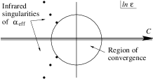
Figure 2: Integration contour and convergence region in the $\ln\epsilon$ plane ($\epsilon=\mu^{2}/Q^{2})$.

To represent Eq. (3) perturbatively, we expand the effective coupling in terms of $\alpha_{\mbox{\tiny S}}(Q^{2})$:

$$\alpha_{\mbox{\tiny eff}}(\mu^{2})=\alpha_{\mbox{\tiny eff}}(e^{z}Q^{2})=\sum_{1}^{n}a_{n}(z)[\alpha_{\mbox{\tiny S}}(Q^{2})]^{n}\;.$$ (4)

This series has some finite region of convergence in the $z$-plane, limited by the positions of the infrared singularities of $\alpha_{\mbox{\tiny eff}}$. If, for example, we use the one-loop expression $\alpha_{\mbox{\tiny eff}}(\mu^{2})=1/b\ln(\mu^{2}/\Lambda^{2})$, then the region is a circle which touches the Landau pole at $z=-\ln(Q^{2}/\Lambda^{2})$. In this case a singularity lies on the contour of integration and the integral is not defined. In a more realistic model for $\alpha_{\mbox{\tiny eff}}$, however, the infrared singularities will lie elsewhere in the complex $z$ plane, as depicted in Fig. 2, and the integral will be unambiguous order by order in $\alpha_{\mbox{\tiny S}}(Q^{2})$. Nevertheless the perturbation series in $\alpha_{\mbox{\tiny S}}(Q^{2})$ will diverge, because the contour extends outside the region of convergence, both to the right and to the left. Since $\dot{\cal F}$ is exponentially damped in $z$ on both sides, while $a_{n}(z)$ is power-behaved, with the power increasing with $n$, the divergence will be of factorial form.

The divergence due to the segment of the contour to the right of the convergence region is called an ultraviolet renormalon. We can see directly from the integral representation (3) that this divergence is just an artefact of expanding in powers of $\alpha_{\mbox{\tiny S}}(Q^{2})$. The ultraviolet contribution to the integral (say, that from $z>0$, i.e. $\mu^{2}>Q^{2}$) is perfectly well defined in terms of the usual perturbative form of the running coupling $\alpha_{\mbox{\tiny eff}}(\mu^{2})\simeq\alpha_{\mbox{\tiny S}}(\mu^{2})$. It can be evaluated numerically, or equivalently the corresponding series can be summed using a standard technique such as Borel summation. The divergence does not originate from the ultraviolet region, being simply a reflection of the limit on the region of convergence set by singularities far away in the infrared.

On the other hand the divergence of the series due to the region on the left, called an infrared renormalon, cannot be eliminated without information on the non-perturbative behaviour of $\alpha_{\mbox{\tiny eff}}$ in the infrared region. It should be clear from Fig. 2 that this ambiguity has nothing to do with whether a Landau pole is present on the axis [6]. It will exist as long as $\alpha_{\mbox{\tiny eff}}$ has any kind of infrared singularities, which it surely must. Therefore the so-called infrared renormalon ambiguity can only be resolved by providing a physical model of the infrared behaviour of $\alpha_{\mbox{\tiny eff}}$. Once this is done, one can integrate unambiguously along the left-hand portion of the contour, since no physical singularities can lie on the $z$-axis (they would correspond to tachyons).

3 Power corrections

Assuming the validity of Eq. (3), we can make useful deductions about the behaviour of $F(Q^{2},x)$ at low $Q^{2}$, without any specific assumptions about the infrared behaviour of the effective coupling. We shall argue that $F$ is of the form

$$F(Q^{2},x)=F^{(n)}_{\mbox{\tiny pert}}(Q^{2},x)+F^{(n)}_{\mbox{\tiny pow}}(Q^{2},x)$$ (5)

where the first term, representing the standard $n$-th order perturbative prediction, has a basically logarithmic $Q^{2}$-dependence while the second, which includes non-perturbative effects, is power-behaved. Note that the second term also requires a superscript $n$ since it depends on where we truncate the perturbation series $F^{(n)}_{\mbox{\tiny pert}}$.

To derive Eq. (5) we split $\alpha_{\mbox{\tiny eff}}$ into two parts, roughly described as perturbative and non-perturbative:

$$\alpha_{\mbox{\tiny eff}}(\mu^{2})=\alpha^{(n)}_{\mbox{\tiny pert}}(\mu^{2})+\delta\alpha^{(n)}_{\mbox{\tiny eff}}(\mu^{2})\;.$$ (6)

The superscript on $\alpha^{(n)}_{\mbox{\tiny pert}}$ indicates that this quantity is obtained by expanding to $n$-th order in $\alpha_{\mbox{\tiny S}}(Q^{2})$:

$$\alpha^{(n)}_{\mbox{\tiny pert}}(\mu^{2}) = \alpha_{\mbox{\tiny S}}(Q^{2})+b\left(\ln\frac{Q^{2}}{\mu^{2}}+K\right)\alpha_{\mbox{\tiny S}}^{2}(Q^{2})$$ (7)

$$+\cdots+{\cal O}\left(\ln\frac{Q^{2}}{\mu^{2}}\right)^{n}\alpha_{\mbox{\tiny S}}^{n}(Q^{2})$$

where the constant $K$ depends on the choice of renormalization scheme. Once again it follows that the remainder $\delta\alpha^{(n)}_{\mbox{\tiny eff}}$ also depends on $n$.

In Fig. 3, the solid curve shows a possible model for the behaviour of $\alpha_{\mbox{\tiny eff}}$, in which it is assumed to vanish at very small scales, as suggested in [7]. Given the present level of understanding, it could equally well approach a non-zero value. The quantity $\delta\alpha^{(n)}_{\mbox{\tiny eff}}$ is given by the difference between the solid curve and the dot-dashed one representing $\alpha^{(n)}_{\mbox{\tiny pert}}$, which rises as $n$ increases. Therefore we expect in general that $\delta\alpha^{(n)}_{\mbox{\tiny eff}}$ will decrease with increasing $n$.

Figure 3: Possible behaviour of the effective coupling. Solid: $\alpha_{\mbox{\tiny eff}}$. Dashed: 1-loop running $\alpha_{\mbox{\tiny S}}$. Dot-dashed: $\alpha^{(n)}_{\mbox{\tiny pert}}$ for $n=2,3,4$.

Substituting in Eq. (3), we obtain Eq. (5) with

$$F^{(n)}_{\mbox{\tiny pow}}=\int_{0}^{\mu_{\mbox{\tiny I}}^{2}}\frac{d\mu^{2}}{\mu^{2}}\,\delta\alpha^{(n)}_{\mbox{\tiny eff}}(\mu^{2})\,\dot{\cal F}(\mu^{2}/Q^{2},x)\;.$$ (8)

We have assumed here that the approximation (7) to $\alpha_{\mbox{\tiny eff}}$ is sufficiently accurate at high $\mu^{2}$ for $\delta\alpha^{(n)}_{\mbox{\tiny eff}}$ to be negligible above some ‘infrared matching’ scale $\mu_{\mbox{\tiny I}}$ ($\Lambda\ll\mu_{\mbox{\tiny I}}\ll Q$). It follows then that the $Q^{2}$ dependence of $F^{(n)}_{\mbox{\tiny pow}}$ is determined by the behaviour of $\dot{\cal F}(\epsilon,x)$ for small values of $\epsilon$. For the general behaviour

$$\dot{\cal F}(\epsilon,x)\sim f(x)\epsilon^{p/2}\ln^{q}\epsilon\;\;\;\;\;\mbox{as}\;\;\epsilon\to 0$$ (9)

we have

$$F^{(n)}_{\mbox{\tiny pow}}\sim\frac{f(x)}{Q^{p}}\int_{0}^{\mu_{\mbox{\tiny I}}^{2}}\frac{d\mu^{2}}{\mu^{2}}\,\delta\alpha^{(n)}_{\mbox{\tiny eff}}(\mu^{2})\,\mu^{p}\,\ln^{q}\left(\frac{\mu^{2}}{Q^{2}}\right)$$ (10)

Thus, as stated earlier, $F^{(n)}_{\mbox{\tiny pow}}$ is power-behaved (modulo logs), with $x$-dependence given by that of $\dot{\cal F}(\epsilon,x)$ at small $\epsilon$ and magnitude determined by a (log-)moment of the ‘effective coupling modification’ $\delta\alpha^{(n)}_{\mbox{\tiny eff}}$.

All this depends only on the validity of the dispersive formula (3), irrespective of whether $\delta\alpha^{(n)}_{\mbox{\tiny eff}}$ varies from one observable $F$ to another. Therefore one would expect the value of the power $p$ to be given reliably by Eq. (9). Under the additional assumption that $\alpha_{\mbox{\tiny eff}}$, and hence $\delta\alpha^{(n)}_{\mbox{\tiny eff}}$, is universal, one obtains testable relationships between power corrections to different observables with the same value of $p$.

Over the last few years, this ‘renormalon-inspired’ or ‘dispersive’ approach to the estimation of power corrections has been applied to a wide variety of QCD observables [5],[8]-[19]. Many of the results have been presented in other talks at this meeting. Therefore I shall concentrate in the remainder of this talk on topics that illustrate some of the general remarks made above.

4 Structure functions

Figure 4: Higher-twist contribution to $F_{2}$ (data, solid curve) and $F_{3}$ (dashed curve).

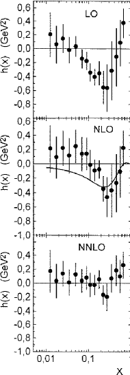
Figure 5: Higher-twist contribution to $F_{3}$, extracted from various orders of perturbative analysis. Figure adapted from Ref. [21].

The need for $1/Q^{2}$ power corrections to hadronic structure functions, normally called higher-twist contributions, is well established and their dependence on the Bjorken $x$ variable has been extracted from deep inelastic scattering (DIS) data. Typical results are shown in Figs. 4 and 5 [20, 21]. In Fig. 4 the higher-twist contribution is parametrized as $D_{2}(x)/Q^{2}$ time the leading-twist, whereas in Fig. 5 it is represented simply as an additive term $h(x)/Q^{2}$.

Such contributions are predicted by the renormalon approach, since the characteristic functions for the evolution of (non-singlet) structure functions have the general form

$$\dot{\cal F}(\epsilon,x)\sim P(x)+f(x)\epsilon\ln\epsilon+\ldots$$ (11)

where $P(x)$ is the usual splitting function and the ellipsis represents terms that are less important as $\epsilon\to 0$. The convolution of the (structure-function-dependent) coefficient function $f(x)$ with the quark distribution then gives the predicted form of the leading $1/Q^{2}$ correction.

The solid curve in Fig. 4 shows the prediction for the structure function $F_{2}$, with the relevant ($p=2$, $q=1$) moment of $\delta\alpha^{(n)}_{\mbox{\tiny eff}}$ (for $n=2$) in Eq. (10) as the only free parameter [5, 14, 17]. The good agreement with the data is due mainly to the characteristic $1/(1-x)$ behaviour at large $x$, which is also predicted by a number of models of higher-twist contributions.

A more stringent test is the prediction of the power correction to $xF_{3}$ [14], which depends on the same moment of $\delta\alpha^{(n)}_{\mbox{\tiny eff}}$. The dashed curve shows the result, for the value of the moment obtained by fitting $F_{2}$. It is interesting that the prediction is negative for all but the largest $x$ values, in agreement with the need for a negative power correction to the GLS sum rule (1). This is confirmed by a recent analysis [21] of the data of the CCFR collaboration [22]: the power corrections extracted in LO, NLO and NNLO (i.e. $n=1,2,3$) analyses are shown in Fig. 5, together with the same prediction for $F_{3}$ as in Fig. 4.

Fig. 5 also illustrates an important point discussed in Sect. 3, namely that the normalization of the power correction depends on the order of the perturbative analysis. It decreases in magnitude with increasing order, as more of the divergent renormalon series is included in the perturbative prediction $F^{(n)}_{\mbox{\tiny pert}}$. We can see from the GLS prediction, Eq. (1), that the perturbative coefficients are indeed increasingly negative, consistent with the presence of an infrared renormalon with a negative coefficient, which tends to cancel the power correction.

5 Event shape variables

Power corrections to hadronic event shapes are generally larger than those in most other observables. This, together with the lack of complete next-to-next-to-leading order perturbative calculations of these quantities, has made it difficult to use them for precise tests of QCD, in spite of the very high statistics available from LEP1.

Usually the non-perturbative contributions to event shapes are estimated using Monte Carlo event generators [23, 24], or rather the hadronization models that are built into them. The difference between the parton- and hadron-level predictions of the generator is taken as the hadronization correction, with an error given by the discrepancy between the models. As discussed in Sect. 1, the trouble with this is that the parton-level generators do not coincide with fixed-order perturbation theory. They represent an approximate summation of various contributions (including the renormalon graphs) up to rather high order. In addition, they contain cutoff parameters that can emulate non-perturbative effects. Thus the power corrections might be under- or over-estimated by this procedure, even though the generator might agree perfectly with the data at the hadron level.

Some less model-dependent insight into power corrections to event shapes can be gained from the renormalon-inspired type of treatment discussed above. Consider as a prototype the thrust variable in $e^{+}e^{-}$ annihilation,

$$T=\max\sum_{i}|{\mbox{\boldmath$p$}}_{i}\cdot{\mbox{\boldmath$n$}}|/\sum_{i}|{\mbox{\boldmath$p$}}_{i}|\;,$$ (12)

where the sum is over final-state hadron momenta ${\mbox{\boldmath$p$}}_{i}$ and the maximum is with respect to the direction of the unit vector $n$ (the thrust axis). In lowest order the difference $1-T$ arises from a $q\bar{q}g$ final state. Making a Sudakov decomposition of the gluon momentum $k$,

$$k=\alpha p+\beta\bar{p}+k_{\perp}$$ (13)

where $p^{2}=\bar{p}^{2}=p\cdot k_{\perp}=\bar{p}\cdot k_{\perp}=0$, $k_{\perp}^{2}=-{\mbox{\boldmath$k$}_{\perp}^{2}}$ and $2p\cdot\bar{p}=Q^{2}$, the c.m. energy-squared, we have

$$t\equiv 1-T=\min\{\alpha,\beta\}$$ (14)

in the soft region. Hence the characteristic function for the mean value of this quantity is

$${\cal F} \simeq \frac{C_{F}}{\pi}\int\frac{d\alpha}{\alpha}\frac{d\beta}{\beta}\,d{\mbox{\boldmath$k$}_{\perp}^{2}}$$ (15)

$$\cdot\min\{\alpha,\beta\}\,\delta(\alpha\beta Q^{2}-{\mbox{\boldmath$k$}_{\perp}^{2}}-\mu^{2})$$

$$= \frac{2C_{F}}{\pi Q}\int\frac{d{\mbox{\boldmath$k$}_{\perp}^{2}}}{\sqrt{{\mbox{\boldmath$k$}_{\perp}^{2}}+\mu^{2}}}\;,$$

from which we find

$$\dot{\cal F}\simeq\frac{2C_{F}}{\pi}\frac{\mu}{Q}\;.$$ (16)

It follows from Eqs. (8) and (16) that the quantity $\langle{t}\rangle$ is expected to receive a $1/Q$ power correction, in contrast to the $1/Q^{2}$ corrections to other quantities like structure and fragmentation [15] functions. A similar result is obtained for the mean values of several other $e^{+}e^{-}$ shape variables [8, 11, 9], and for the corresponding quantities in deep inelastic final states [16].

There is by now good experimental evidence for $1/Q$ corrections to the mean values of several event shape variables in both $e^{+}e^{-}$ annihilation [25, 26] and DIS [27]. Furthermore the magnitudes of the corrections are in most cases consistent (at about the 20% level) with a universal value of the relevant moment of $\delta\alpha^{(n=2)}_{\mbox{\tiny eff}}$ in Eq. (10), namely

$$\int\frac{d\mu^{2}}{\mu^{2}}\,\mu\,\delta\alpha^{(n=2)}_{\mbox{\tiny eff}}(\mu^{2})\simeq 1\;\mbox{GeV}\;.$$ (17)

Turning from the mean values to the distributions of event shape variables, a simple result is obtained when the dominant low-momentum contributions exponentiate, that is, when they correspond to essentially uncorrelated multiple soft gluon emission. This is the case for the thrust distribution, which may be expressed as a Laplace transform [28]

$$F(t)\equiv\frac{1}{\sigma}\frac{d\sigma}{dt}=\int_{C}d\nu\,\exp[\nu t+R(\nu,Q)]$$ (18)

where the contour $C$ runs parallel to the imaginary axis, to the right of all singularities of the integrand, and $t=1-T$ as usual. The ‘radiator’ $R$ has the following form in lowest order:

$$R(\nu,Q) = \frac{2C_{F}}{\pi}\int\frac{d\mu^{2}}{\mu^{2}}\alpha_{\mbox{\tiny eff}}(\mu^{2})$$ (19)

$$\cdot\int_{\mu^{2}/Q^{2}}^{\mu/Q}\frac{du}{u}\left(\mbox{e}^{-u\nu}-1\right)$$

To compute the effect of a non-perturbative contribution to $\alpha_{\mbox{\tiny eff}}$, confined to the region $\mu^{2}<\mu_{\mbox{\tiny I}}^{2}\ll Q^{2}$, we note that, since $\nu$ is conjugate to $t$, the exponential can safely be expanded to first order as long as $t\gg\mu_{\mbox{\tiny I}}/Q$. The resulting change in the radiator is

$$\delta R\simeq-\frac{2C_{F}}{\pi}\nu\int\frac{d\mu^{2}}{\mu^{2}}\delta\alpha^{(n)}_{\mbox{\tiny eff}}(\mu^{2})\frac{\mu}{Q}\equiv-\nu\frac{A}{Q}$$ (20)

which corresponds simply to a shift in the $t$-distribution [9, 13], by an amount $A/Q$ equal to the non-perturbative shift in $\langle{t}\rangle$ computed above:

$$F(t)\simeq F_{\mbox{\tiny pert}}(t-A/Q)$$ (21)

where $F_{\mbox{\tiny pert}}$ is the perturbative prediction. This agrees well with the $e^{+}e^{-}$ data [13].

There is some ambiguity in the calculations outlined above: we assumed an effective gluon mass $\mu$ but used the massless forms of the shape variable and lowest-order matrix element, when expressed in terms of the Sudakov variables $\alpha$ and $\beta$, as was done in [8]. In reality the ‘massive’ gluon fragments into massless partons, which eventually form hadrons, and the fragmentation products may have a thrust value different from that of their parent [12]. This will not change the $1/Q$ form of the power correction but it would be expected to modify its coefficient.

These issues have been clarified in a recent paper from the Milan group [29], in which the coefficient of the $1/Q$ correction is evaluated to two-loop order in the soft limit. A substantial increase, relative to the above naive treatment, is obtained – a factor of 1.8 for three active flavours. Interestingly, however, this enhancement factor itself appears to be universal across a wide range of shape variables, in both $e^{+}e^{-}$ and DIS final states [30]. Therefore the experimental analyses [25, 26, 27] of event shapes assuming universality are not invalidated, but the fitted values of the moments of $\delta\alpha^{(n)}_{\mbox{\tiny eff}}$, such as Eq. (17), need to be rescaled by the inverse of the Milan factor.

6 Better shape variables

As we have seen, the power corrections to event shapes are normally of order $1/Q$. For determinations of $\alpha_{\mbox{\tiny S}}$, it would be an advantage to know if there are any shape variables that are free of such corrections, preferably up to order $1/Q^{2}$.

One set of variables that has been suggested is the higher moments of shape variables. A straightforward approach along the lines of Sect. 3 suggests that if the mean value has a correction of order $1/Q$ then the $p$-th moment will only receive a non-perturbative contribution of order $1/Q^{p}$.

Unfortunately the situation is not so simple, since we would also like to safeguard against corrections of order $\alpha_{\mbox{\tiny S}}(Q^{2})/Q\gg 1/Q^{2}$. Consider again for example the variable $t\equiv 1-T$. We know that the power correction to the NLO perturbative prediction for $\langle{t}\rangle$ is $A/Q$ where $A\simeq 1$ GeV. Furthermore we saw that the main non-perturbative effect on the thrust distribution $F(t)$ is a simple shift, Eq. (21). It follows that for the mean value of $t^{p}$ we have

$$\langle{t^{p}}\rangle = \int dt\,t^{p}F(t)\simeq\int dt\,(t+A/Q)^{p}F_{\mbox{\tiny pert}}(t)$$ (22)

$$= \langle{t^{p}}\rangle_{\mbox{\tiny pert}}+\frac{pA}{Q}\langle{t^{p-1}}\rangle_{\mbox{\tiny pert}}+{\cal O}\left(\frac{1}{Q^{2}}\right)$$

In practice, the perturbative predictions for $\langle{t^{p}}\rangle$ decrease rapidly with $p$, and therefore the second term is relatively important for $p>1$, in spite of its suppression by $\alpha_{\mbox{\tiny S}}(Q^{2})$. One finds

$$\langle{t}\rangle_{\mbox{\tiny pert}} = 0.335\alpha_{\mbox{\tiny S}}+1.03\alpha_{\mbox{\tiny S}}^{2}+\ldots\;,$$

$$\langle{t^{2}}\rangle_{\mbox{\tiny pert}} = 0.030\alpha_{\mbox{\tiny S}}+0.15\alpha_{\mbox{\tiny S}}^{2}+\ldots\;.$$ (23)

and so, at LEP energies and below, the power corrections to $\langle{t}\rangle$ and $\langle{t^{2}}\rangle$ are actually comparable, relative to the perturbative predictions. In addition, the perturbation series for $\langle{t^{2}}\rangle$ and higher moments show increasingly poor convergence.

A better idea is to consider moments about the mean value, such as the thrust variance $\sigma^{2}_{\mbox{\tiny T}}=\langle{t^{2}}\rangle-\langle{t}\rangle^{2}$. Then we see from Eq. (22) that the $\alpha_{\mbox{\tiny S}}(Q^{2})/Q$ corrections should cancel out. Furthermore the perturbative prediction,

$$\sigma^{2}_{\mbox{\tiny T, pert}}=0.030\alpha_{\mbox{\tiny S}}+0.04\alpha_{\mbox{\tiny S}}^{2}+\ldots\;,$$ (24)

shows better convergence than that for $\langle{t^{2}}\rangle$ – better than $\langle{t}\rangle$, in fact. Nevertheless, this is a quantity an order of magnitude smaller than $\langle{t}\rangle$, and so its measurement will require that experimental sources of error are well under control.

An interesting open question is whether the $1/Q$ and $\alpha_{\mbox{\tiny S}}(Q^{2})/Q$ corrections to $\sigma^{2}_{\mbox{\tiny T}}$ remain cancelled after taking into account the Milan enhancement factor, to be extracted from a two-loop analysis.

Finally we should consider a shape variable which is not expected to have $1/Q$ or $\alpha_{\mbox{\tiny S}}(Q^{2})/Q$ corrections to its first moment, namely the three-jet resolution $y_{3}$. This is the value of the Durham jet measure $y_{\mbox{\tiny cut}}$ at which three jets are just resolved in the final state. Recalling that the Durham criterion for resolving two partons $i$ and $j$ is $y_{ij}>y_{\mbox{\tiny cut}}$, where [31]

$$y_{ij}=2\min\{E_{i}^{2},E_{j}^{2}\}(1-\cos\theta_{ij})/Q^{2}\;,$$ (25)

we find that in the soft limit we obtain in place of Eq. (14)

$$y_{3}=(\alpha+\beta)\min\{\alpha,\beta\}\;,$$ (26)

giving instead of Eq. (16)

$$\dot{\cal F}\simeq\frac{2C_{F}}{\pi}\frac{\mu^{2}}{Q^{2}}\ln\left(\frac{Q}{\mu}\right)$$ (27)

for $\langle{y_{3}}\rangle$. Thus, modulo possible logarithms, the expected leading correction to this quantity is ${\cal O}(1/Q^{2})$. Once again, it would be interesting to know whether the Milan enhancement can somehow generate a $1/Q$ correction. Experimentally, no significant power correction to $\langle{y_{3}}\rangle$ has yet been found [26], which is certainly consistent with the absence of a $1/Q$ term.

7 Conclusions

The renormalon-inspired or dispersive method for estimating power corrections to perturbative calculations of QCD observables has proved to be a useful phenomenological tool. At the very least, it warns us of those quantities and phase-space regions in which the perturbative calculation is dangerously sensitive to low-momentum contributions. If we wish, we can simply avoid those regions in comparing theory with experiment. From this viewpoint, the renormalon ambiguity is analogous to the renormalization-scale dependence of a next-to-leading order perturbative prediction: if it is large, we would be unwise to trust the prediction as a reliable test of QCD or as a good way of measuring $\alpha_{\mbox{\tiny S}}$. The ideal observable for these purposes has both a small scale dependence and a small renormalon ambiguity – in particular, a large value of the power $p$. These are somewhat independent requirements, and therefore a renormalon analysis provides useful additional information, even if we do not accept it as a quantitative estimate of power corrections.

As far as I am aware, the powers $p$ for the corrections observed experimentally agree with those predicted in all cases studied so far. This provides the motivation for going further and comparing the measured and computed coefficients of power corrections, assuming a universal low-energy form for the effective strong coupling $\alpha_{\mbox{\tiny eff}}$. The initial results look encouraging to me, although many issues remain unclear. As emphasised in Sect. 4, the coefficient must depend on the order of the perturbative prediction that is being subtracted. Presumably the optimal comparison would be with the perturbation series truncated at its smallest term, but we remain far from that situation. In the case of event shape variables, the renormalization of the coefficient by two-loop effects has been shown to be large but appears to remain universal for a range of observables. A general argument can be made that higher loop corrections should be small [29], but explicit calculations would be reassuring.

Another relevant question is whether we should expect the strong coupling itself to exhibit power corrections, possibly as large as $1/Q^{2}$ [32]. There have been recent suggestions of such terms in lattice calculations [33]. A systematic perturbative treatment of the effective strong coupling beyond one-loop (i.e. one-renormalon-chain) order seems essential for this purpose, but is still lacking. Approaches such as that of [34] may be fruitful. Such a treatment would also be valuable for the study of power corrections to gluon-dominated quantities such as hadronic jet shapes [35] and small-$x$ structure functions [36].

References

- [1] For reviews and classic references see V.I. Zakharov, Nucl. Phys. B385 (1992) 452 and A.H. Mueller, in QCD 20 Years Later, vol. 1 (World Scientific, Singapore, 1993).
- [2] M. Beneke and V.M. Braun, Phys. Lett. 348B (1995) 513 (hep-ph/9411229); P. Ball, M. Beneke and V.M. Braun, Nucl. Phys. B452 (1995) 563 (hep-ph/9502300).
- [3] M. Neubert, Phys. Rev. D51 (1995) 5924 (hep-ph/9412265).
- [4] F. Di Renzo, E. Onofri and G. Marchesini, Nucl. Phys. B457 (1995) 202 (hep-th/9502095).
- [5] Yu.L. Dokshitzer, G. Marchesini and B.R. Webber, Nucl. Phys. B469 (1996) 93 (hep-ph/9512336).
- [6] Yu.L. Dokshitser and N.G. Uraltsev, Phys. Lett. 380B (1996) 141 (hep-ph/9512407); G. Grunberg, Ecole Polytechnique preprint CPTH-S505-0597 (hep-ph/9705290).
- [7] Yu.L. Dokshitzer, V.A. Khoze and S.I. Troyan, Phys. Rev. D53 (1996) 89 (hep-ph/9506425).
- [8] B.R. Webber, Phys. Lett. 339B (1994) 148 (hep-ph/9408222); see also Proc. Summer School on Hadronic Aspects of Collider Physics, Zuoz, Switzerland, 1994 (hep-ph/9411384).
- [9] G.P. Korchemsky and G. Sterman, Nucl. Phys. B437 (1995) 415 (hep-ph/9411211); in Proc.30th Rencontres de Moriond, Meribel les Allues, France, March 1995 (hep-ph/9505391); G.P. Korchemsky, G. Oderda and G. Sterman, Stony Brook preprint ITP-SB-97-41, to appear in Proc. DIS97 (hep-ph/9708346).
- [10] Yu.L. Dokshitzer and B.R. Webber, Phys. Lett. 352B (1995) 451 (hep-ph/9504219).
- [11] R. Akhoury and V.I. Zakharov, Phys. Lett. 357B (1995) 646 (hep-ph/9504248); Nucl. Phys. B465 (1996) 295 (hep-ph/9507253).
- [12] P. Nason and M.H. Seymour, Nucl. Phys. B454 (1995) 291 (hep-ph/9506317).
- [13] Yu.L. Dokshitzer and B.R. Webber, Phys. Lett. 404B (1997) 321 (hep-ph/9704298).
- [14] M. Dasgupta and B.R. Webber, Phys. Lett. 382B (1996) 273 (hep-ph/9604388).
- [15] M. Dasgupta and B.R. Webber, Nucl. Phys. B484 (1997) 247 (hep-ph/9608394); P. Nason and B.R. Webber, Phys. Lett. 395B (1997) 355 (hep-ph/9612353); M. Beneke, V.M. Braun and L. Magnea, Nucl. Phys. B497 (1997) 297 (hep-ph/9701309).
- [16] M. Dasgupta and B.R. Webber, Cavendish-HEP-96/5, to appear in Z. Phys. C (hep-ph/9704297).
- [17] E. Stein, M. Meyer-Hermann, L. Mankiewicz and A. Schäfer, Phys. Lett. 376B (1996) 177 (hep-ph/9601356); M. Meyer-Hermann, M. Maul, L. Mankiewicz, E. Stein and A. Schäfer, Phys. Lett. 383B (1996) 463, erratum ibid. B393 (1997) 487 (hep-ph/9605229).
- [18] M. Maul, E. Stein, A. Schäfer and L. Mankiewicz, Phys. Lett. 401B (1997) 100 (hep-ph/9612300); M. Maul, E. Stein, L. Mankiewicz, M. Meyer-Hermann and A. Schäfer, hep-ph/9710392.
- [19] M. Meyer-Hermann and A. Schäfer, hep-ph/9709349.
- [20] M. Virchaux and A. Milsztajn, Phys. Lett. 274B (1992) 221.
- [21] A.L. Kataev, A.V. Kotikov, G. Parente and A.V. Sidorov, Dubna preprint JINR-E2-97-194 (hep-ph/9706534).
- [22] CCFR Collaboration, P.Z. Quintas et al., Phys. Rev. Lett. 71 (1997) 1307; CCFR-NuTeV Collaboration, W.G. Seligman et al., Columbia preprint Nevis-292 (hep-ex/9701017).
- [23] T. Sjöstrand, Comp. Phys. Commun. 82 (1994) 74 (hep-ph/9508391).
- [24] G. Marchesini, B.R. Webber, G. Abbiendi, I.G. Knowles, M.H. Seymour, L. Stanco, Comp. Phys. Commun. 67 (1992) 465 (hep-ph/9607393).
- [25] DELPHI Collaboration, P. Abreu et al., Z. Phys. C73 (1997) 22; D. Wicke, in Proc. QCD97, Montpellier, July 1997 (hep-ph/9708467).
- [26] JADE Collaboration, P.A. Movilla Fernandez et al., Aachen preprint PITHA-97-27 (hep-ex/9708034); O. Biebel, Aachen preprint PITHA-97-32 (hep-ex/9708036).
- [27] H1 Collaboration, C. Adloff et al., Phys. Lett. 406B (1997) 256 (hep-ex/9706002).
- [28] S. Catani, L. Trentadue, G. Turnock and B.R. Webber, Phys. Lett. 263B (1991) 491; Nucl. Phys. B407 (1993) 3.
- [29] Yu.L. Dokshitzer, A. Lucenti, G. Marchesini and G.P. Salam, Milan preprint IFUM-573-FT (hep-ph/9707532).
- [30] Yu.L. Dokshitzer, A. Lucenti, G. Marchesini and G.P. Salam, Milan preprint in preparation; M. Dasgupta and B.R. Webber, Cambridge preprint in preparation.
- [31] Yu.L. Dokshitzer, contribution cited in Report of the Hard QCD Working Group, Proc. Workshop on Jet Studies at LEP and HERA, Durham, December 1990, J. Phys. G17 (1991) 1537.
- [32] R. Akhoury and V.I. Zakharov, Michigan preprint UM-TH-97-11 (hep-ph/9705318); G. Grunberg, preprint CERN-TH/97-340 (hep-ph/9711481).
- [33] G. Burgio, F. Di Renzo, G. Marchesini and E. Onofri, to appear in Proc. Lattice 97, Edinburgh, July 1997 (hep-lat/9709105).
- [34] N.J. Watson, Nucl. Phys. B494 (1997) 388 (hep-ph/9606381).
- [35] M.H. Seymour, Rutherford preprint RAL-TR-97-026 (hep-ph/9707338).
- [36] F. Hautmann, Oregon preprint OITS-640 (hep-ph/9710256).