The $\mathchar 259\relax$-parameter and $m_{s}$ of quenched QCD¹

Abstract.

We explain how scale dependent renormalized quantities can be computed using lattice QCD. Two examples are used: the running coupling and quark masses. A reliable computation of the $\mathchar 259\relax$-parameter in the quenched approximation is presented.

DESY 97-223

1 Introduction

In a perturbative treatment, one takes as parameters of QCD the running coupling and running quark masses in a specific renormalization scheme. If we adopt a mass-independent scheme, the coupling and quark masses satisfy rather simple renormalization group equations. Their asymptotic high energy behavior is given by the $\mathchar 259\relax$-parameter and the renormalization group invariant masses $\{M_{f}\}$ ($f$ labeling the flavors). These parameters have the advantage that $M_{f}$ are independent of the renormalization scheme and the $\mathchar 259\relax$-parameters of different schemes can be related exactly by 1-loop calculations.

Once one considers QCD on the non-perturbative level, it is natural to take $N_{\rm f}+1$ hadronic observables to be the parameters that fix the theory instead of $\mathchar 259\relax$ and $\{M_{f}\}$. We call this a hadronic scheme (HS). For QCD with $u$ and $d$ taken as mass-degenerate and an additional $s$-quark, one may take for example the proton mass, $m_{\rm p}$, the pion mass, $m_{\pi}$, and the Kaon mass, $m_{\rm K}$, as the basic parameters. Of course, the two sets of parameters are related once a non-perturbative solution of QCD is available. It is a challenge for lattice QCD to provide this relation with completely controlled errors. In this brief report we describe a method that allows to solve this problem. The numerical results (sect. 4) are for quenched QCD, i.e. the fermion determinant is omitted in the path integral; one may think of this as a version of QCD with $N_{\rm f}=0$ flavors of sea-quarks.

The problem described above is the connection of the short distance and long distance dynamics of QCD. As such it appears at first sight to be intractable by numerical simulations, since it requires that various scales are treated on one and the same lattice. This is impossible, if discretization errors are supposed to be under control! However, one may define a running coupling and running quark masses in QCD in a finite volume of linear size $L$ with suitably chosen boundary conditions (cf. sect. 3). Then the masses and coupling run with an energy scale $q=1/L$ and their evolution can be computed recursively. The only requirement to keep discretization errors small in each step of the recursion is $L\gg a$ which is easy to satisfy ($a$ denotes the lattice spacing)[1, 2].

2 Strategy

We start by giving an overview of the strategy to compute short distance parameters in figure1.

$${L_{\rm max}}={\rm O}(\hbox{$1\over 2$}\hbox{$.\!\!^{\rm m}$}):\qquad{\rm HS}\quad\longrightarrow\quad {\rm SF}(q=1/{L_{\rm max}})$$

$$\downarrow$$

$${\rm SF}(q=2/{L_{\rm max}})$$

$$\downarrow$$

$$\bullet$$

$$\bullet$$

$$\bullet$$

$$\downarrow$$

$${\rm SF}(q=2^{n}/{L_{\rm max}})$$

$$\mbox{ PT:}\quad\downarrow\qquad\quad$$

$${\rm jet-physics}\quad\stackrel{{\scriptstyle\rm PT}}{{\longleftarrow}}\quad \mathchar 259\relax_{\rm QCD},M$$

Fig. 1.: The strategy for a non-perturbative computation of short distance parameters.

One first renormalizes QCD replacing the bare parameters by hadronic observables. This defines the HS introduced above. It can be related to the finite volume scheme (denoted by SF) at a low energy scale $q=1/L_{\rm max}$, where $L_{\rm max}$ is of the order of $1\penalty 10000\kern 3.0pt\hbox{$.\!\!^{\rm m}$}$. Within this scheme one then computes the scale evolution up to a desired energy $q=2^{n}/{L_{\rm max}}$. It is no problem to choose the number of steps $n$ large enough to be sure that one has entered the perturbative regime. There perturbation theory (PT) is used to evolve further to infinite energy and compute $\mathchar 259\relax$ and $\{M_{f}\}$. Inserted into perturbative expressions, these parameters provide predictions for jet cross sections or other high energy observables. In figure1, all arrows correspond to relations in continuum QCD; the whole strategy is designed such that lattice calculations for these relations can be extrapolated to the continuum limit.

For the practical success of the approach, the finite volume coupling and quark masses must satisfy a number of criteria.

• They should have an easy perturbative expansion, such that the $\beta$-function (and $\tau$-function, which describes the evolution of the running masses) can be computed to sufficient order in the coupling.

• They should be easy to calculate in MC (small variance!).

• Lattice effects must be small to allow for safe extrapolations $a/L\to 0$.

Careful consideration of the above points led to the introduction of the running coupling, $\bar{g}$, and quark mass, $\kern 1.0pt\overline{\kern-1.0ptm\kern-1.0pt}\kern 1.0pt$, through the Schrödinger functional (SF) of QCD [3, 2, 4, 5].

3 Schrödinger functional scheme

We describe the definition of $\bar{g}$ and $\kern 1.0pt\overline{\kern-1.0ptm\kern-1.0pt}\kern 1.0pt$ in a formal continuum formulation. The SF is the partition function of the Euclidean path integral on a hyper-cylinder with Dirichlet boundary conditions in time, ($P_{\pm}=\hbox{$1\over 2$}(1\pm\gamma_{0})$)

$$\left.\begin{array}[]{llll}A_{k}(x)=C_{k}({\bf x}),&P_{+}\psi(x)=\rho({\bf x}),&\overline{\psi}(x)P_{-}=\bar{\rho}({\bf x})&\mbox{at}\,\,x_{0}=0\enspace,\\ A_{k}(x)=C^{\prime}_{k}({\bf x}),&P_{-}\psi(x)=\rho^{\prime}({\bf x}),&\overline{\psi}(x)P_{+}=\bar{\rho}^{\prime}({\bf x})&\mbox{at}\,\,x_{0}=L\enspace.\end{array}\right.$$ (3)

Here, $A_{k},\ldots,\bar{\rho}^{\prime}$ are classical prescribed boundary fields. In space, the gauge fields are taken periodic under shifts $x\to x+L\hat{k}$ and the fermion fields are periodic up to a phase $\theta$.

The renormalized coupling is defined through the response of the SF to an infinitesimal change of the boundary gauge fields $C_{k},C_{k}^{\prime}$. Since the boundary fields are taken with a strength proportional to $1/L$, there is no scale apart from $L$ and the coupling $\bar{g}(L)$ runs with $L$. Details have been discussed in several publications [3, 2].

A natural starting point for the definition of a renormalized quark mass is the PCAC relation,

$$\partial_{\mu}A_{\mu}^{a}(x)=2mP^{a}(x)\enspace,$$ (4)

which expresses the proportionality of the divergence of the axial current, $A_{\mu}^{a}$, to the pseudo-scalar density $P^{a}$, where

$$P^{a}(x)=\overline{\psi}(x)\gamma_{5}\hbox{$1\over 2$}\tau^{a}\psi(x),\quad A_{\mu}^{a}=\overline{\psi}(x)\gamma_{\mu}\gamma_{5}\hbox{$1\over 2$}\tau^{a}\psi(x)\enspace,$$ (5)

and $\tau^{a}$ are the Pauli-matrices acting in flavor space (we take $N_{\rm f}=2$ degenerate flavors from now on). Renormalizing the operators in equation 4,

$$(A_{{\rm R}})_{\mu}^{a}=Z_{\rm A}A_{\mu}^{a}\enspace,\quad P_{{\rm R}}^{a}=Z_{\rm P}P^{a}\enspace,$$ (6)

we define a renormalized quark mass by

$$\kern 1.0pt\overline{\kern-1.0ptm\kern-1.0pt}\kern 1.0pt={Z_{\rm A}\over Z_{\rm P}}m\enspace.$$ (7)

Here, $m$ is to be taken from equation 4 inserted into an arbitrary correlation function. It does not depend on the chosen correlation function, since equation 4 is an operator identity. The scale independent renormalization $Z_{\rm A}$ can be fixed through current algebra relations (also in the lattice regularization [6, 7]) and we are left to give a normalization condition for the pseudo-scalar density, $P_{{\rm R}}$. The running mass, $\kern 1.0pt\overline{\kern-1.0ptm\kern-1.0pt}\kern 1.0pt$, then inherits its scheme- and scale-dependence from the corresponding dependence of $P_{{\rm R}}$.

We define $Z_{\rm P}$ in terms of correlation functions in the SF.

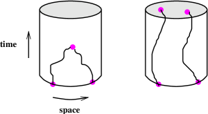
Fig. 2.: $.\!\!^{\scriptscriptstyle\rm p}$ (left) and $f_{1}$ (right) in terms of quark propagators.

To start, we construct (isovector) pseudo-scalar fields at the boundary of the SF ,

$${\cal O}^{a} = \int{\rm d}^{3}{\bf u}\int{\rm d}^{3}{\bf v}\,\,\bar{\zeta}({\bf u})\gamma_{5}\hbox{$1\over 2$}\tau^{a}\zeta({\bf v})\enspace,$$ (8)

from the “boundary quark fields”, $\zeta,\bar{\zeta}$. Their precise definition [8] involves a functional derivative, e.g. $\zeta({\bf x})\equiv\hbox{$\delta\over\delta\bar{\rho}({\bf x})$}$. After taking this functional derivative one sets the boundary values, $\rho...$ ,to zero. Analogously one defines a field ${\cal O}^{\prime a}$, which resides at $x_{0}=L$. These fields are used in the correlation functions

$$\hbox{$.\!\!^{\scriptscriptstyle\rm p}$}(x_{0})=-\hbox{$1\over 3$}\langle P^{a}(x){\cal O}^{a}\rangle\enspace,\quad f_{1} = \langle{\cal O}\kern-7.7778pt\kern 7.7778pt\smash{\raise 4.5pt\hbox{\kern 1.0pt$\scriptstyle\prime$}}\kern 1.0pt^{a}{\cal O}^{a}\rangle\enspace,$$ (9)

(see figure2). In the ratio

$$Z_{\rm P}={\rm const.}\sqrt{f_{1}}/\hbox{$.\!\!^{\scriptscriptstyle\rm p}$}(x)|_{x_{0}=L/2}\enspace,$$ (10)

the renormalization of the boundary quark fields [4] cancels out; it can therefore be taken as the definition of the renormalization constant of $P$. The proportionality constant is to be chosen such that $Z_{\rm P}=1$ at tree level. Further details of the definition are $C=C^{\prime}=0$ and a specific choice for $\theta$. The renormalization constant is to be evaluated for zero quark mass, $m$. This defines a mass-independent scheme.

By construction, the SF scheme is non-perturbative and independent of a specific regularization. For a concrete non-perturbative computation, we do, however, need to evaluate the expectation values by a MC-simulation of the corresponding lattice theory. For the details of the lattice formulation we refer to [8] but mention that it is essential to use an ${\rm O}(a)$-improved formulation in order to keep lattice spacing effects small [9]. We now explain the computation of the scale dependence, omitting the matching to the HS scheme [2, 5] for lack of space.

4 Scale evolution, $\mathchar 259\relax$ and RGI masses

Each step in the recursive computation of the scale evolution consists of:

• Choose a lattice with $L/a$ points in each direction.

• Tune the bare coupling, $g_{0}$, such that the renormalized coupling $\bar{g}^{2}(L)$ has the value $u$ and tune the bare mass, $m_{0}$, such that the mass (equation 4) vanishes; compute $Z_{\rm P}$.

• At the same values of $g_{0},m_{0}$, simulate a lattice with twice the linear size; compute $u^{\prime}=\bar{g}^{2}(2L)$ and $Z_{\rm P}^{\prime}$. This determines the lattice step scaling functions for the coupling, $\mathchar 262\relax(u,a/L)$=u’, and for the mass, $\mathchar 262\relax_{\rm P}(u,a/L)=Z_{\rm P}/Z_{\rm P}^{\prime}$.

• Repeat steps 1.–3. with different resolutions $L/a$ and extrapolate $\sigma(u)=\lim_{a/L\to 0}\mathchar 262\relax(u,a/L)$, $\sigma_{\rm P}(u)=\lim_{a/L\to 0}\mathchar 262\relax_{\rm P}(u,a/L)$. This extrapolation can be done by allowing for small linear $a/L$-discretization errors [2].

Fig. 3.: Non-perturbative running coupling and quark mass as a function of $q\equiv 1/L$. Uncertainties are smaller than the size of the symbols.

In this way, $\sigma(u),\,1.1\leq u\leq 2.4$ and $\sigma_{\rm P}(u),\,1.1\leq u\leq 3.48$ have been computed in the quenched approximation. The scale evolution is monotonous in this range: $\sigma(u)>u$, $\sigma_{\rm P}(u)>1$. $\sigma$ and $\sigma_{\rm P}$ can therefore be used to follow figure1 downwards (up in the energy scale).

Starting from the box size $L_{\rm max}$, defined by $\bar{g}^{2}(L_{\rm max})=3.48$, we use

$$\bar{g}^{2}(L_{k-1})=\sigma(\bar{g}^{2}(L_{k})),\,\,\,\kern 1.0pt\overline{\kern-1.0ptm\kern-1.0pt}\kern 1.0pt(L_{k-1})=\sigma_{\rm P}(\bar{g}^{2}(L_{k}))\,\kern 1.0pt\overline{\kern-1.0ptm\kern-1.0pt}\kern 1.0pt(L_{k}),\,\,\,L_{k}=2^{-k}L_{\rm max}$$ (11)

to compute the sequences [5]

$$\bar{g}^{2}(L_{k}),\quad\kern 1.0pt\overline{\kern-1.0ptm\kern-1.0pt}\kern 1.0pt(L_{k})/\kern 1.0pt\overline{\kern-1.0ptm\kern-1.0pt}\kern 1.0pt(L_{\rm max}),\quad k=0,1,\ldots 8\enspace.$$ (12)

In figure3, these are compared to the perturbative evolutions (starting at the weakest coupling). It is surprising that the perturbative evolution is quite precise down to rather low energy scales. This property may of course not be generalized to other schemes but has to be checked in each scheme separately.

On the other hand, the figure clearly demonstrates that the SF-scheme is perturbative in the large energy regime, say $q>50{\rm GeV}$. We may therefore start from the exact relations

$$\mathchar 259\relax = q\left(b_{0}\bar{g}^{2}\right)^{-b1/(2b_{0}^{2})}{\rm e}^{-1/(2b_{0}\bar{g}^{2})}\exp\left\{-\int_{0}^{\bar{g}}{\rm d}x\left[\hbox{$1\over\beta(x)$}+\hbox{$1\over b_{0}x^{3}$}-\hbox{$b_{1}\over b_{0}^{2}x$}\right]\right\}\enspace,$$ (13)

$$M = \kern 1.0pt\overline{\kern-1.0ptm\kern-1.0pt}\kern 1.0pt\,(2b_{0}\bar{g}^{2})^{-d_{0}/2b_{0}^{2}}\exp\left\{-\int_{0}^{\bar{g}}{\rm d}g[\hbox{$\tau(g)\over\beta(g)$}-\hbox{$d_{0}\over b_{0}g$}]\right\}\enspace,$$ (14)

insert for the $\beta$-function ($\tau$-function) its 3-loop (2-loop) approximation and set $q$ to the maximal value reached, to compute $\mathchar 259\relax$ and $\kern 1.0pt\overline{\kern-1.0ptm\kern-1.0pt}\kern 1.0pt/M$. One can easily convince oneself that the left over perturbative uncertainty is negligible compared to the accumulated statistical errors.

After converting to the $\overline{\rm MS}$-scheme one arrives at the result[5]

$$\mathchar 259\relax_{\overline{\rm MS}}^{(0)}=251\pm 21{\rm MeV}\enspace,$$ (15)

where the label ⁽⁰⁾ reminds us that this number was obtained with zero quark flavors. The error in equation 15 accounts for all uncertainties including the extrapolations to the continuum limit that were done in the intermediate steps.

This talk is based on research done in the framework of the ALPHA collaboration[5]. I thank in particular S. Capitani, M. Guagnelli, M. Lüscher, S. Sint, P. Weisz and H. Wittig for the joint work.

References

- [1] M. Lüscher, P. Weisz and U. Wolff, Nucl. Phys. B359 (1991) 221
- [2] M. Lüscher, R. Sommer, P. Weisz and U. Wolff, Nucl. Phys. B389 (1993) 247, Nucl. Phys. B413 (1994) 481
- [3] M. Lüscher, R. Narayanan, P. Weisz and U. Wolff, Nucl. Phys. B384 (1992) 168
- [4] S. Sint, Nucl. Phys. B421 (1994) 135, Nucl. Phys. B451 (1995) 416
- [5] S. Capitani et al., hep-lat/9709125
- [6] M. Bochicchio, L. Maiani, G. Martinelli, G.C. Rossi and M. Testa, Nucl. Phys. B262 (1985) 331
- [7] M. Lüscher, S. Sint, R. Sommer and H. Wittig, Nucl. Phys. B491 (1997) 344
- [8] M. Lüscher, S. Sint, R. Sommer and P. Weisz, Nucl. Phys. B478 (1996) 365
- [9] R. Sommer, -improved lattice QCD, hep-lat/9705026