SUSY–QCD Corrections to
Higgs Particle Decays into Quarks and Squarks

Abstract

We study the decays of the Higgs bosons $H^{\pm}$, $H^{0}$, and $A^{0}$ within the Minimal Supersymmetric Standard Model. For decays into quarks and squarks we include the supersymmetric QCD radiative corrections. We find that the corrections are significant and can go up to 50%. The supersymmetric decay modes $H^{+}\rightarrow\tilde{t}\bar{\tilde{b}}$ and $H^{0}(A^{0})\rightarrow\tilde{t}\bar{\tilde{t}}$ can be dominant in a wide range of the model parameters due to the large Yukawa couplings and mixings of $\tilde{t}$ and $\tilde{b}$.

1 Introduction

We need to find the Higgs boson for a conclusive test of the electroweak symmetry breaking mechanism of the Standard Model. The search for the Higgs boson, therefore, has high priority at LEP, TEVATRON, LHC, and a future $e^{+}e^{-}$ Linear Collider. To facilitate searching for the Higgs boson we need to study not only the production mechanisms, but also all possible decay modes. While in the Standard Model (SM) there is only one physical Higgs particle, extensions of the SM contain more Higgs bosons.

In this contribution we consider Higgs particle decays in the Minimal Supersymmetric Standard Model (MSSM) $\!{}^{{\bf?}}$. The MSSM implies the existence of five physical Higgs bosons $h^{0}$, $H^{0}$, $A^{0}$, and $H^{\pm}$ $\!{}^{{\bf?},{\bf?}}$. Provided that all SUSY particles are very heavy, the $H^{+}$ decays mainly into $t\bar{b}$, and below the $t\bar{b}$ threshold the decays $H^{+}\to\tau^{+}\nu$ and/or $H^{+}\to W^{+}h^{0}$ are dominant $\!{}^{{\bf?},{\bf?}}$. Similarly, if all decay modes of $H^{0}$ and $A^{0}$ into SUSY particles are kinematically forbidden, they decay dominantly into a fermion pair of the third generation. Higgs boson decays into supersymmetric (SUSY) particles can be very important if they are kinematically allowed. The decays into charginos and neutralinos can have large branching ratios, and can significantly change the signatures of SUSY Higgs particles $\!{}^{{\bf?},{\bf?}}$. The decays into squarks can be the dominant decay modes of Higgs bosons in a large parameter region in case that the squarks are relatively light $\!{}^{{\bf?},{\bf?}}$.

For a precise determination of the Higgs boson couplings to quarks and squarks we need to include the SUSY–QCD corrections in the calculation of the decay widths. The SUSY–QCD corrections in ${\cal O}(\alpha_{s})$ were calculated in the on–shell scheme for the processes $H^{+}\to t\bar{b}$ in $\!{}^{{\bf?},{\bf?}}$, and for $H^{0},A^{0}\to q\bar{q}$ in $\!{}^{{\bf?}}$. For the decays of Higgs particles into squark pairs we calculated the SUSY–QCD corrections in the on–shell scheme in $\!{}^{{\bf?}}$, including squark–mixing and a proper renormalization of the mixing angle $\theta_{\tilde{q}}$ $\!{}^{{\bf?}}$. The SUSY–QCD corrections to Higgs boson decays into squarks were also studied in $\!{}^{{\bf?}}$ recently.

In this talk we review our work on the branching ratios of Higgs boson decays. In order to show how the branching ratios of the various decay modes depend on the SUSY parameters, we will first summarize the tree–level results. Then we will take into account the SUSY–QCD corrections in ${\cal O}(\alpha_{s})$ for the decay branching ratios into third generation quarks and squarks. We will show that in most cases the SUSY–QCD corrections are significant and need to be included.

At tree–level the masses of the MSSM Higgs bosons depend on the two parameters $m_{A}$ and $\tan\beta$. $m_{A}$ is the mass of the pseudoscalar Higgs boson $A^{0}$, and $\tan\beta=\frac{v_{2}}{v_{1}}$ is the ratio of the vacuum expectation values of the two neutral Higgs doublet states $\!{}^{{\bf?},{\bf?}}$. The mass of $h^{0}$ gets large radiative corrections from one–loop contributions. We will take into account these corrections using the formulae of $\!{}^{{\bf?}}$. The experimental lower bounds on the Higgs boson masses from LEP are $m_{h^{0}}>62$ GeV and $m_{A^{0}}>62$ GeV $\!{}^{{\bf?}}$. In addition to $\tan\beta$, the main SUSY parameters in the chargino and neutralino systems are the Higgs–higgsino mass parameter $\mu$ and the $SU(2)$ gaugino mass parameter $M$. We assume that $M$ is related to the gluino mass $m_{{\tilde{g}}}$ and the $U(1)$ gaugino mass parameter $M^{\prime}$ by $M=(\alpha_{2}/\alpha_{s}(m_{\tilde{g}}))m_{{\tilde{g}}}=3/(5\tan^{2}\theta_{W})M^{\prime}$. For the third generation squarks and sleptons we also need the mass parameters $M_{\tilde{Q}}$, $M_{\tilde{U}}$, $M_{\tilde{D}}$, $M_{\tilde{L}}$, $M_{\tilde{E}}$, and the trilinear scalar coupling parameters $A_{t}$, $A_{b}$ and $A_{\tau}$.

2 Tree–Level Widths

In the following we will use the short–hand notation $H^{k}$, $k=1,2,3,4$, for the Higgs bosons of the MSSM, with $H^{1}\equiv h^{0}$, $H^{2}\equiv H^{0}$, $H^{3}\equiv A^{0}$, and $H^{4}\equiv H^{+}$. The decay widths for $H^{k}\rightarrow q\bar{q}$, $k=1,2,3$, $q=t,b$, and $H^{+}\rightarrow t\bar{b}$ are given by

$$\Gamma^{tree}(H^{k}\rightarrow q\bar{q}) = \frac{3g^{2}m_{q}^{2}(d_{k}^{q})^{2}m_{H^{k}}}{32\pi m_{W}^{2}\,a_{q}^{2}}\left(1-\frac{4m_{q}^{2}}{m_{H^{k}}^{2}}\right)^{(3/2-\delta_{k3})}\!\!\!\!\!\!\!\!(k=1,2,3),$$ (1)

$$\Gamma^{tree}(H^{+}\rightarrow t\bar{b}) = \frac{3\kappa(m_{H^{+}}^{2},m_{t}^{2},m_{b}^{2})}{16\pi m_{H^{+}}^{3}}\times$$ (2)

$$\left[(m_{H^{+}}^{2}-m_{t}^{2}-m_{b}^{2})(y_{t}^{2}+y_{b}^{2})-4m_{t}m_{b}y_{t}y_{b}\right]\,,$$

with $\kappa(x,y,z)\equiv((x-y-z)^{2}-4yz)^{1/2}$, $d_{1}^{t}=d_{2}^{b}=\cos\alpha$, $d_{2}^{t}=-d_{1}^{b}=-\sin\alpha$, $d_{3}^{t}=a_{b}=\cos\beta$, $d_{3}^{b}=-a_{t}=-\sin\beta$, where $\alpha$ is the mixing angle in the $h^{0}$ – $H^{0}$ system $\!{}^{{\bf?},{\bf?}}$. $y_{t}$ and $y_{b}$ are related to the Yukawa couplings and are $y_{t}=h_{t}\cos\beta=gm_{t}\cot\beta/(\sqrt{2}m_{W})$ and $y_{b}=h_{b}\sin\beta=gm_{b}\tan\beta/(\sqrt{2}m_{W})$. The decay widths into top quarks are large due to the large top quark mass. If $\tan\beta>20$, the decay modes into bottom quarks can also become important. Asymptotically for $m_{H^{k}}\gg m_{q}$ the Higgs boson decay widths into quarks are proportional to $m_{H^{k}}$.

The Higgs boson decay widths into squarks of the third generation depend on ${\tilde{q}}_{L}-{\tilde{q}}_{R}$ mixing. This mixing is described by the squark mass matrix which in the basis (${\tilde{q}}_{L}$, ${\tilde{q}}_{R}$), ${\tilde{q}}={\tilde{t}}$ or ${\tilde{b}}$, and in the diagonalized form is

$$\left(\begin{array}[]{cc}m_{LL}^{2}&m_{LR}^{2}\\ m_{RL}^{2}&m_{RR}^{2}\end{array}\right)=(R^{{\tilde{q}}})^{\dagger}\left(\begin{array}[]{cc}m_{{\tilde{q}}_{1}}^{2}&0\\ 0&m_{{\tilde{q}}_{2}}^{2}\end{array}\right)R^{{\tilde{q}}}\,,$$ (3)

where $R^{{\tilde{q}}}_{i\alpha}$ is a $2\times 2$ rotation matrix with rotation angle $\theta_{\tilde{q}}$, and

$$m_{LL}^{2} = M_{\tilde{Q}}^{2}+m_{q}^{2}+m_{Z}^{2}\cos 2\beta(I^{3L}_{q}-e_{q}\sin^{2}\theta_{W})\,,$$ (4)

$$m_{RR}^{2} = M_{\{\tilde{U},\tilde{D}\}}^{2}+m_{q}^{2}+m_{Z}^{2}\cos 2\beta\,e_{q}\sin^{2}\theta_{W}\,,$$ (5)

$$m_{LR}^{2} = m_{RL}^{2}=m_{q}(A_{q}-\mu(\tan\beta)^{-2I^{3L}_{q}})\,.$$ (6)

$I^{3L}_{q}$ and $e_{q}$ are the third component of isospin and the electric charge of the quark $q$, and $\theta_{W}$ is the Weinberg angle. The mass eigenstates ${\tilde{q}}_{i},i=1,2$, ($m_{{\tilde{q}}_{1}}<m_{{\tilde{q}}_{2}}$) are related to the states ${\tilde{q}}_{\alpha},\alpha=L,R$, by ${\tilde{q}}_{i}=R^{{\tilde{q}}}_{i\alpha}{\tilde{q}}_{\alpha}$.

The widths of the decays $H^{k}\rightarrow{\tilde{q}}_{i}\bar{{\tilde{q}}}_{j}$ at tree–level are

$$\Gamma^{tree}(H^{k}\rightarrow{\tilde{q}}_{i}\bar{{\tilde{q}}}_{j})=\frac{3\kappa(m_{H^{k}}^{2},m_{{\tilde{q}}_{i}}^{2},m_{{\tilde{q}}_{j}}^{2})}{16\pi m_{H^{k}}^{3}}|G_{ijk}^{\tilde{q}}|^{2}\,.$$ (7)

For $k=1,2,3$ we have ${\tilde{q}}={\tilde{t}},{\tilde{b}}$, and for $k=4$ we have ${\tilde{q}}_{i}\equiv{\tilde{t}}_{i}$, ${\tilde{q}}_{j}\equiv{\tilde{b}}_{j}$, $(i,j=1,2)$. The expressions for the couplings $G_{ijk}^{\tilde{q}}$ are given in $\!{}^{{\bf?}}$. The Higgs boson decay widths into squarks can be large in the case of large squark mixing. For example, the width of $A^{0}\rightarrow{\tilde{q}}_{1}\bar{{\tilde{q}}}_{2}$ is directly proportional to $|m_{q}(A_{q}(\tan\beta)^{-2I^{3L}_{q}}+\mu)|^{2}$. The same expressions appear in the couplings $G_{ij4}$ for the decays $H^{+}\rightarrow{\tilde{t}}_{i}\bar{{\tilde{b}}}_{j}$. The $H^{0}{\tilde{t}}_{i}{\tilde{t}}_{j}$ couplings can be large since they contain terms proportional to $m_{t}$, and the $H^{0}{\tilde{b}}_{i}{\tilde{b}}_{j}$ couplings can be large if $\tan\beta>20$. More details can be found in $\!{}^{{\bf?}}$. For $m_{H^{k}}\gg m_{{\tilde{q}}_{i}}$ the widths of Higgs boson decays into squarks behave asymptotically like $1/m_{H^{k}}$.

In the calculation of the corresponding branching ratios we have included the widths of the following $H^{+}$, $H^{0}$ and $A^{0}$ decay modes:
(i) $H^{+}$ $\to$ $t\bar{b}$, $c\bar{s}$, $\tau^{+}\nu_{\tau}$, $W^{+}h^{0}$, ${\tilde{t}}_{i}\bar{\tilde{b}}_{j}$, $\tilde{\chi}^{+}_{k}\tilde{\chi}^{0}_{l}$, $\tilde{\tau}_{i}^{+}\tilde{\nu}_{\tau}$, $\tilde{\ell}_{L}^{+}\tilde{\nu}_{\ell}\,(\ell=e,\mu)$, (ii) $H^{0}$ $\to$ $t\bar{t}$, $b\bar{b}$, $c\bar{c}$, $\tau^{-}\tau^{+}$, $W^{+}W^{-}$, $Z^{0}Z^{0}$, $h^{0}h^{0}$, $A^{0}A^{0}$, $W^{\pm}H^{\mp}$, $Z^{0}A^{0}$, ${\tilde{t}}_{i}\bar{{\tilde{t}}}_{j}$, ${\tilde{b}}_{i}\bar{{\tilde{b}}}_{j}$, ${\tilde{\ell}}^{-}_{i}{\tilde{\ell}}^{+}_{j}$, ${\tilde{\nu}}_{\ell}\bar{{\tilde{\nu}}}_{\ell}$ ($\ell=e,\mu,\tau$), ${\tilde{\chi}}^{+}_{i}{\tilde{\chi}}^{-}_{j}$, ${\tilde{\chi}^{0}}_{k}{\tilde{\chi}^{0}}_{l}$, and (iii) $A^{0}$ $\to$ $t\bar{t}$, $b\bar{b}$, $c\bar{c}$, $\tau^{-}\tau^{+}$, $Z^{0}h^{0}$, ${\tilde{t}}_{1}\bar{{\tilde{t}}}_{2}$, ${\tilde{t}}_{2}\bar{{\tilde{t}}}_{1}$, ${\tilde{b}}_{1}\bar{{\tilde{b}}}_{2}$, ${\tilde{b}}_{2}\bar{{\tilde{b}}}_{1}$, ${\tilde{\tau}}^{-}_{1}{\tilde{\tau}}^{+}_{2}$, ${\tilde{\tau}}^{-}_{2}{\tilde{\tau}}^{+}_{1}$, ${\tilde{\chi}}^{+}_{i}{\tilde{\chi}}^{-}_{j}$, ${\tilde{\chi}^{0}}_{k}{\tilde{\chi}^{0}}_{l}$.

Formulae for these widths are found e. g. in $\!{}^{{\bf?}}$. We have not taken into account loop induced decay modes like $H^{+}\to W^{+}Z^{0},W^{+}\gamma$, $H^{0}\to gg,\gamma\gamma$ etc., and three-body decay modes $\!{}^{{\bf?},{\bf?}}$.

We have shown in $\!{}^{{\bf?},{\bf?}}$ that the branching ratios for decays into squarks, $H^{+}\to{\tilde{t}}_{i}\bar{{\tilde{b}}}_{j}$, $H^{0}\to{\tilde{t}}_{i}\bar{{\tilde{t}}}_{j},{\tilde{b}}_{i}\bar{{\tilde{b}}}_{j}$, and $A^{0}\to{\tilde{t}}_{1}\bar{{\tilde{t}}}_{2},{\tilde{b}}_{1}\bar{{\tilde{b}}}_{2}$ can be larger than $50\%$ in a sizeable region of the SUSY parameter space. To illustrate this we show in Figs. 2a, and c the tree level decay widths (dashed lines) $\Gamma(H^{0}\to{\tilde{t}}\bar{{\tilde{t}}})\equiv\sum_{i,j}\Gamma(H^{0}\to{\tilde{t}}_{i}\bar{{\tilde{t}}}_{j})$ and $\Gamma(A^{0}\to{\tilde{t}}_{1}\bar{{\tilde{t}}}_{2})$ as a function of $m_{A}$. For comparison we also show in Figs. 2a and c the tree level decay widths $\Gamma(H^{0}\to t\bar{t})$ and $\Gamma(A^{0}\to t\bar{t})$ (dashed lines). Fig. 3a shows the tree level decay widths $\Gamma(H^{+}\to{\tilde{t}}\bar{{\tilde{b}}})\equiv\sum_{i,j}\Gamma(H^{+}\to{\tilde{t}}_{i}\bar{{\tilde{b}}}_{j})$ and $\Gamma(H^{+}\to t\bar{b})$ as a function of $m_{A}$ (dashed lines). In these plots we have assumed the relations $M_{\tilde{Q}}:M_{\tilde{U}}:M_{\tilde{D}}=1:\frac{8}{9}:\frac{10}{9}$ for the squark mass parameters, and $A\equiv A_{t}=A_{b}$ for the trilinear scalar coupling parameters. We have taken $M_{\tilde{Q}}=120$ GeV, $A=280$ GeV, $\mu=300$ GeV, $M=140$ GeV, and $\tan\beta=3$. In the plots we have required $m_{h^{0}}>70$ GeV. For large $m_{A^{0}}$ one has $m_{H^{+}}\approx m_{H^{0}}\approx m_{A^{0}}$. For this set of parameters we have (in GeV) ($m_{{\tilde{t}}_{1}}$, $m_{{\tilde{t}}_{2}}$, $m_{{\tilde{b}}_{1}}$, $m_{{\tilde{b}}_{2}}$, $m_{{\tilde{g}}}$, $m_{\tilde{\chi}_{1}^{0}}$, $m_{\tilde{\chi}_{1}^{+}}$) = (102, 271, 121, 145, 412, 63, 116). In the examples shown, the decay widths $\Gamma(H^{0}\to{\tilde{t}}\bar{{\tilde{t}}})$, $\Gamma(A^{0}\to{\tilde{t}}_{1}\bar{{\tilde{t}}}_{2})$, and $\Gamma(H^{+}\to{\tilde{t}}\bar{{\tilde{b}}})$ are always much larger than the decay widths $\Gamma(H^{0}\to t\bar{t})$, $\Gamma(A^{0}\to t\bar{t})$, and $\Gamma(H^{+}\to t\bar{b})$, respectively. The corresponding branching ratios for decays into third generation squarks are much larger than 50% in the whole $m_{A}$ range shown where these decays are kinematically allowed. The branching ratios for the decays into sbottoms, $H^{0}\to{\tilde{b}}_{i}\bar{{\tilde{b}}}_{j}$ and $A^{0}\to{\tilde{b}}_{1}\bar{{\tilde{b}}}_{2}$ turn out to be less than 3% due to the low $\tan\beta$ value considered.

3 SUSY–QCD Corrected Decay Widths

In Section 2 we have seen that the Higgs boson decays into squarks can be important. Therefore, it is necessary to include the SUSY–QCD radiative corrections in the calculation of the widths for the decays into squarks and into quarks. In this section we will review some of our results about the branching ratios of Higgs boson decays including the SUSY–QCD corrections in ${\cal O}(\alpha_{s})$. For further details concerning the theoretical calculation of these corrections we refer to $\!{}^{{\bf?},{\bf?},{\bf?},{\bf?},{\bf?}}$.

The Feynman diagrams for the virtual ${\cal O}(\alpha_{s})$ SUSY–QCD corrections are shown in Fig. 1. We work in the on–shell renormalization scheme. We first discuss the radiative corrections for the Higgs boson decays into squarks. In this case the virtual corrections consist of the vertex corrections, wave function corrections, and the corrections due to the shift from the bare couplings to the on–shell couplings. We use the scheme introduced in $\!{}^{{\bf?}}$ for $e^{+}e^{-}\to{\tilde{q}}_{i}\bar{\tilde{q}}_{j}$, where we fixed the counterterm of the squark mixing angle such that it cancels the off–diagonal term of the squark wave–function correction to $e^{+}e^{-}\to{\tilde{q}}_{1}\bar{\tilde{q}}_{2}$. For the shift $\delta\theta_{\tilde{q}}$ we take the same expression as in $\!{}^{{\bf?}}$. A more detailed discussion of the on–shell renormalization of the squark mixing angle $\theta_{\tilde{q}}$ is given in $\!{}^{{\bf?}}$.

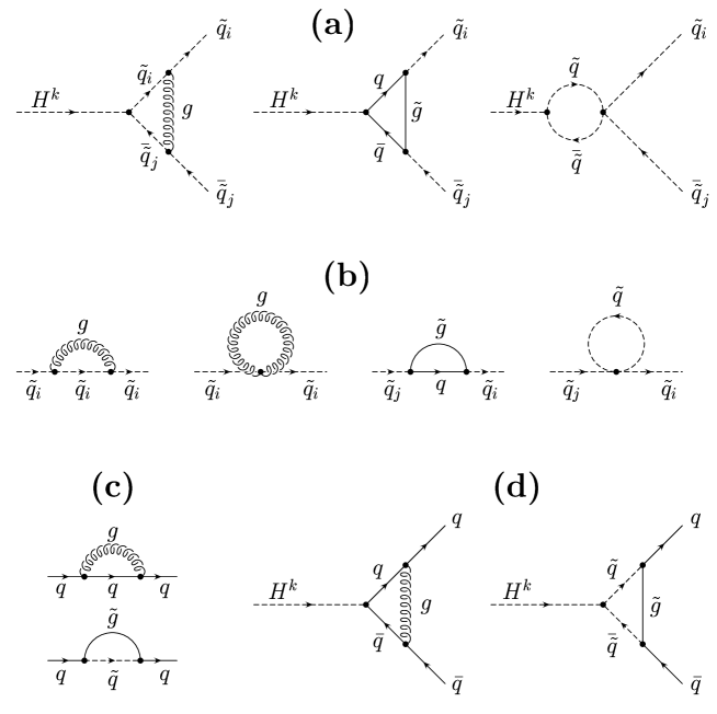
Figure 1: Feynman diagrams for the calculation of the virtual ${\cal O}(\alpha_{s})$ SUSY–QCD corrections to the decay widths $H^{k}\to{\tilde{q}}_{i}\bar{\tilde{q}}_{j}$ and $H^{k}\to q\bar{q}$.

The calculation of the SUSY–QCD corrections to the decay widths of $H^{+}\to{\tilde{t}}\bar{{\tilde{b}}}$ and of the branching ratios of $H^{0}$ and $A^{0}$ decays involves both the stop and the sbottom sector. We have to pay special attention to the parameter $M_{\tilde{Q}}$ in the on–shell scheme. $SU(2)_{L}$ symmetry requires that at tree–level and in the $\overline{DR}$ scheme the parameter $M_{\tilde{Q}}$ is the same in the stop and sbottom mass matrix (see eq.(4)). However, in the on–shell scheme this is no more the case, because the shifts from the $\overline{DR}$ parameters to the on–shell parameters are, in general, different for the stop and sbottom sectors. In the present case we choose $M_{\tilde{Q}}({\tilde{t}})|_{OS}$ in the stop sector as the on–shell input parameter. Then $M_{\tilde{Q}}({\tilde{b}})|_{OS}$ in the sbottom sector is shifted by the amount

$$M^{2}_{\tilde{Q}}({\tilde{b}})|_{OS}=M^{2}_{\tilde{Q}}({\tilde{t}})|_{OS}+\delta M^{2}_{\tilde{Q}}({\tilde{t}})-\delta M^{2}_{\tilde{Q}}({\tilde{b}})\,.$$ (8)

The shift $\delta M^{2}_{\tilde{Q}}({\tilde{t}})-\delta M^{2}_{\tilde{Q}}({\tilde{b}})$ is ultra–violet finite due to the underlying $SU(2)_{L}$ symmetry.

We also include the SUSY–QCD corrections for the Higgs decays into third generation quarks, taking the formulae of $\!{}^{{\bf?},{\bf?},{\bf?}}$. In the following numerical examples we assume for the on–shell input parameters the same relations as for the tree–level quantities, $M_{\tilde{Q}}({\tilde{t}}):M_{\tilde{U}}:M_{\tilde{D}}:M_{\tilde{L}}:M_{\tilde{E}}=1:\frac{8}{9}:\frac{10}{9}:1:1$ and $A\equiv A_{t}=A_{b}=A_{\tau}$. We take $m_{t}=175$ GeV, $m_{b}=5$ GeV, $m_{Z}=91.2$ GeV, $m_{W}=80$ GeV, $\sin^{2}\theta_{W}=0.23$, $\alpha_{2}=0.0337$, and $\alpha_{s}=\alpha_{s}(m_{H^{k}})$ for $H^{k}$ decay. We use $\alpha_{s}(Q)=12\pi/\{(33-2n_{f})\ln(Q^{2}/\Lambda_{n_{f}}^{2})\}$, with $\alpha_{s}(m_{Z})=0.12$, and the number of quark flavors $n_{f}=5(6)$ for $m_{b}<Q\leq m_{t}$ (for $Q>m_{t}$).

In addition to the tree–level decay width we show in Fig. 2a also the SUSY–QCD corrected decay width $\sum_{i,j}\Gamma(H^{0}\to{\tilde{t}}_{i}\bar{{\tilde{t}}}_{j})$ and $\Gamma(H^{0}\to t\bar{t})$ as a function of $m_{A}$ (full lines). In Fig. 2c we show also the SUSY–QCD corrected widths $\Gamma(A^{0}\to{\tilde{t}}_{1}\bar{{\tilde{t}}}_{2})$ and $\Gamma(A^{0}\to t\bar{t})$, and in Fig. 3a those of $\sum_{i,j}\Gamma(H^{+}\to{\tilde{t}}_{i}\bar{{\tilde{b}}}_{j})$ and $\Gamma(H^{+}\to t\bar{b})$. We have taken $M_{\tilde{Q}}({\tilde{t}})=120$ GeV, and for $A,M,\mu$, and $\tan\beta$ the same values as in the tree–level calculation. The masses of ${\tilde{t}}_{1}$, ${\tilde{t}}_{2}$, ${\tilde{g}}$, $\tilde{\chi}_{1}^{0}$, and $\tilde{\chi}_{1}^{+}$ are the same as mentioned at the end of Section 2, however, those of ${\tilde{b}}_{1}$ and ${\tilde{b}}_{2}$ are different due to eq. (8). For the parameters used we get $M_{\tilde{Q}}({\tilde{b}})=134$ GeV, $m_{{\tilde{b}}_{1}}=127$ GeV, and $m_{{\tilde{b}}_{2}}=151$ GeV. This means that the shift $(M_{\tilde{Q}}({\tilde{b}})-M_{\tilde{Q}}({\tilde{t}}))|_{OS}$ at one–loop level is about 10% of the tree–level value of $M_{\tilde{Q}}$. As can be seen in Figs. 2a, c and Fig. 3a, the corrections to the sums of the decay widths $\sum_{i,j}\Gamma(H^{0}\to{\tilde{t}}_{i}\bar{\tilde{t}}_{j})$, $\sum_{i,j}\Gamma(H^{+}\to{\tilde{t}}_{i}\bar{\tilde{b}}_{j})$, and to $\Gamma(A^{0}\to{\tilde{t}}_{1}\bar{\tilde{t}}_{2})$ are significant and can be larger than 30%. The modes into bottom quarks and sbottoms are very small compared to the top and stop modes and are not shown. In Figs. 2b and d we show the SUSY–QCD corrected branching ratios for $H^{0}$ and $A^{0}$ decays into squarks, quarks, charginos and neutralinos, and in Fig. 3b those for $H^{+}$ decays. In the examples shown the squark decay modes are always the dominant ones. The discontinuities in $\sum_{i,j}\Gamma(H^{0}\to{\tilde{t}}_{i}\bar{\tilde{t}}_{j})$ and $\sum_{i,j}\Gamma(H^{+}\to{\tilde{t}}_{i}\bar{\tilde{b}}_{j})$, and in the corresponding branching ratios, are due to decay channels opening.

Figure 2: Tree–level and SUSY–QCD corrected decay widths into squarks and quarks ((a) and (c)) and important branching ratios ((b) and (d)) for the neutral Higgs boson decays, $H^{0},A^{0}\to\sum_{i,j=1,2}({\tilde{t}}_{i}\bar{\tilde{t}}_{j}+{\tilde{b}}_{i}\bar{\tilde{b}}_{j})$ (full line), $H^{0},A^{0}\to t\bar{t}+b\bar{b}$ (dashed line), and $H^{0},A^{0}\to\sum_{i,j=1,2}\tilde{\chi}_{i}^{+}\tilde{\chi}_{j}^{-}+\sum_{i,j=1,4}\tilde{\chi}_{i}^{0}\tilde{\chi}_{j}^{0}$ (dashed–dotted line), as functions of $m_{A^{0}}$.

Figure 3: (a) tree–level and SUSY–QCD corrected decay widths into squarks and quarks and (b) important branching ratios for the charged Higgs boson decays, $H^{+}\to\sum_{i,j=1,2}{\tilde{t}}_{i}\bar{\tilde{b}}_{j}$ (full line), $H^{+}\to t\bar{b}$ (dashed line), and $H^{+}\to\sum_{i=1,2}\sum_{j=1,4}\tilde{\chi}_{i}^{+}\tilde{\chi}_{j}^{0}$ (dashed–dotted line), as functions of $m_{A^{0}}$.

The SUSY–QCD corrections to the widths of individual decay modes into squarks, $H^{0}\to{\tilde{t}}_{i}\bar{\tilde{t}}_{j}$ or $H^{+}\to{\tilde{t}}_{i}\bar{\tilde{b}}_{j}$, may go up to 50%. They may also be negative. When summed over the individual decay channels, the SUSY–QCD corrections to $\sum_{i,j}\Gamma(H^{0}\to{\tilde{t}}_{i}\bar{\tilde{t}}_{j})$ and $\sum_{i,j}\Gamma(H^{+}\to{\tilde{t}}_{i}\bar{\tilde{b}}_{j})$ are in many cases positive, whereas those for the decays into quarks are in general negative. Therefore, in these cases the branching ratios for decays into squarks are enhanced by including the SUSY–QCD corrections.

We also studied the $m_{\tilde{t}_{1}}$ and $\mu$ dependence of the tree–level and SUSY–QCD corrected branching ratios. Figs. 4a and b show the branching ratios $\sum_{i,j}B(H^{0}\to{\tilde{t}}_{i}\bar{{\tilde{t}}}_{j})$ and $B(A^{0}\to{\tilde{t}}_{1}\bar{{\tilde{t}}}_{2})$ as a function of $m_{\tilde{t}_{1}}$ by varying $M_{\tilde{Q}}=M_{\tilde{Q}}({\tilde{t}})$, taking $m_{A}=600$ GeV, $\mu=300$ GeV, $M=140$ GeV, $\tan\beta=3$, and $A=280$ GeV. Figs. 5a and b show the same branching ratios as a function of $\mu$, taking $M_{\tilde{Q}}=120$ GeV, and the remaining parameters as in Figs. 3. For $\mu<500$ GeV the branching ratios for $H^{0}$ and $A^{0}$ decays into squarks increase with increasing $\mu$. This is a consequence of the $\mu$–dependence of the widths for the decays into charginos and neutralinos.

References

Figure 4: Tree–level and SUSY–QCD corrected branching fractions of the neutral Higgs bosons $H^{0}$ and $A^{0}$ decaying into squarks, as a function of $m_{{\tilde{t}}_{1}}$.

Figure 5: Tree–level and SUSY–QCD corrected branching fractions of the neutral Higgs bosons $H^{0}$ and $A^{0}$ decaying into squarks, as functions of $\mu$.

References

[1]
H. E. Haber and G. L. Kane, Phys. Rep. 117 (1985) 75.
[2]
J. F. Gunion, H. E. Haber, G. L. Kane, and S. Dawson,
The Higgs Hunter’s Guide, Addison-Wesley (1990).
[3]
J. F. Gunion and H. E. Haber, Nucl. Phys. B272
(1986) 1; B402 (1993) 567 (E).
[4]
Z. Kunszt and F. Zwirner, Nucl. Phys. B385 (1992) 3.
[5]
H. Baer, D. Dicus, M. Drees and X. Tata, Phys. Rev. D36 (1987)
1363;
J. Gunion and H. Haber, Phys. Rev. D37 (1988) 2515;
A. Djouadi, J. Kalinowski and P. Zerwas, Z. Phys. C57 (1993)
569;
J. Gunion and J. Kelly, Phys. Rev. D56 (1997) 1730.
[6]
A. Djouadi, J. Kalinowski, P. Ohmann and P. Zerwas,
Z. Phys. C74 (1997) 93.
[7]
A. Bartl, K. Hidaka, Y. Kizukuri, T. Kon and W. Majerotto,
Phys. Lett. B315 (1993) 360.
[8]
A. Bartl, H. Eberl, K. Hidaka, T. Kon, W. Majerotto, and Y. Yamada,
Phys. Lett. B389 (1996) 538.
[9]
A. Bartl, H. Eberl, K. Hidaka, T. Kon, W. Majerotto, and Y. Yamada,
Phys. Lett. B378 (1996) 167, and references therein.
[10]
R. A. Jiménez and J. Solà, Phys. Lett. B389 (1996) 53.
[11]
J. A. Coarasa, R. A. Jiménez, and J. Solà,
Phys. Lett. B389 (1996) 312.
[12]
A. Bartl, H. Eberl, K. Hidaka, T. Kon, W. Majerotto, and Y. Yamada,
Phys. Lett. B402 (1997) 303, and references therein.
[13]
H. Eberl, A. Bartl and W. Majerotto,
Nucl. Phys. B472 (1996) 481.
[14]
A. Arhrib, A. Djouadi, W. Hollik and C. Jünger,
hep-ph/9702426.
[15]
Y. Okada, M. Yamaguchi and T. Yanagida, Progr. Theor. Phys. 85
(1991) 1;
H. Haber and R. Hempfling, Phys. Rev. Lett. 66 (1991) 1815;
J. Ellis, G. Ridolfi and F. Zwirner, Phys. Lett. B257 (1991) 83;
R. Barbieri, F. Caravaglios and M. Frigeni, Phys. Lett. B258
(1991) 167.
[16]
ALEPH Collaboration, Preprint CERN–PPE/97–071, subm. to
Phys. Lett. B.
[17]
J. F. Gunion, G. L. Kane and J. Wudka, Nucl. Phys. B299 (1988)
231;
M. C. Peyranère, H. E. Haber and P. Irulegui, Phys. Rev. D44
(1991) 191.
A. Mèndez and A. Pomarol, Nucl. Phys. B349 (1991) 369.
[18]
A. Djouadi, J. Kalinowski and P. M. Zerwas,
Z. Phys. C70 (1996) 435.
[19]
W. Majerotto, these Proceedings.