LU TP 97-35

November 1997

Transverse and Longitudinal
Bose-Einstein Correlations in $\mbox{e}^{+}\mbox{e}^{-}$ annihilation

Markus Ringnér

Department of Theoretical Physics, Lund University,

Sölvegatan 14A, S-223 62 Lund, Sweden

Abstract:
We show how a difference in the correlation length longitudinally and transversely, with respect to the jet axis in $e^{+}e^{-}$ annihilation, arises naturally in a model for Bose-Einstein correlations based on the Lund string model. The difference is more apparent in genuine three-particle correlations and they are therfore a good probe for the longitudinal stretching of the string field.

(To appear in The Proceedings of the EPS Conference HEP97, Jerusalem, August 1997)

Abstract.

We show how a difference in the correlation length longitudinally and transversely, with respect to the jet axis in $e^{+}e^{-}$ annihilation, arises naturally in a model for Bose-Einstein correlations based on the Lund string model. The difference is more apparent in genuine three-particle correlations and they are therefore a good probe for the longitudinal stretching of the string field.

1 Introduction

Bosons obey Bose-Einstein statistics, which compared to an uncorrelated production leads to an enhancement of the production of identical bosons at small momentum separations. The enhancement is called the Bose-Einstein effect and it is very often parametrised in the form

$$R_{2}(q)=1+\lambda\exp(-Q^{2}R^{2})$$ (1)

where Q is the relative four-momenta of a pair of bosons, $Q^{2}=-q^{2}=-(p_{2}-p_{1})^{2}$, and $R$ and $\lambda$ are two phenomenological parameters. The parameter $R$ is often refered to as the radius of the boson emitting source. It is clear that the correlation function $R_{2}$ reflects the space–time region in which the particle production occurs but both the parametrisation in equation1 and the interpretation of $R$ are often given without very convincing arguments.

In reference[1] (an extension of reference[2] to multi-boson final states) a model for Bose-Einstein correlations based on a quantum-mechanical interpretation of the Lund string fragmentation model [3] is presented. In this work we will investigate some features of the model to see how the correlation lengths in the model arises and this will be used to show what the parameter $R$ is sensitive to. We will in particular show that the model predicts, due to the properties of string fragmentation, a difference between the correlation length along the string and transverse to it. In practice this means that if we introduce the longitudinal and transverse components of the vector $q$ (defined with respect to the thrust axis in $\mbox{e}^{+}\mbox{e}^{-}$ annihilation) we obtain a noticable difference in the correlation distributions. This becomes even more apparent when we go to three-particle correlations because in this case one is even more sensitive to the longitudinal stretching of the string field.

2 Correlation lengths

The starting point of our Bose-Einstein model [1, 2] is an interpretation of the (non-normalised) Lund string area fragmentation probability for an $n$-particle state (see figure1)

$$dP(p_{1},p_{2},\ldots,p_{n})=\penalty 10000\kern 3.0pt\penalty 10000\kern 3.0pt\penalty 10000\kern 3.0pt\penalty 10000\kern 3.0pt\penalty 10000\kern 3.0pt\penalty 10000\kern 3.0pt\penalty 10000\kern 3.0pt\penalty 10000\kern 3.0pt\penalty 10000\kern 3.0pt\penalty 10000\kern 3.0pt\penalty 10000\kern 3.0pt\penalty 10000\kern 3.0pt\penalty 10000\kern 3.0pt\penalty 10000\kern 3.0pt\penalty 10000\kern 3.0pt\penalty 10000\kern 3.0pt$$ (2)

$$\prod_{1}^{n}\!Ndp_{j}\delta(p_{j}^{2}\!-\!m_{j}^{2})\delta(\sum p_{j}\!-\!P_{tot})exp(-bA)$$

in accordance with a quantum mechanical transition probability containing the final state phase space multiplied with the square of a matrix element ${\cal M}$. In reference[2] and in more detail in reference[1] a possible matrix element is suggested in agreement with (Schwinger) tunneling and the (Wilson) loop operators necessary to ensure gauge invariance. The matrix element is

$${\cal M}=\exp(i\kappa-b/2)A$$ (3)

where the area A is interpreted in coordinate space, $\kappa\simeq 1$ GeV/fm is the string constant and $b\simeq 0.3$ GeV/fm is the decay constant.

The transverse momentum properties are in the Lund model taken into account by means of a Gaussian tunneling process. The produced $(\mbox{q}\overline{\mbox{q}})$-pair in each vertex will in this way obtain $\pm\bf{k}_{\perp}$ and the hadron stemming from the combination of a $\overline{\mbox{q}}$ from one vertex and a q from the adjacent vertex obtains $\bf{p}_{\perp}=\bf{k}_{\perp j+1}-\bf{k}_{\perp j}$.

In case there are two or more identical bosons the matrix element should be symmetrised and in general we obtain the symmetrised production amplitude

$${\cal M}=\sum_{{\cal P}}{\cal M_{{\cal P}}}$$ (4)

where the sum goes over all possible permutations of identical particles. Taking the square we get

$$|{\cal M}|^{2}\!=\!\sum_{{\cal P}}|{\cal M}_{{\cal P}}|^{2}\!\left(\!1\!+\!\!\sum_{{\cal P}^{\prime}\neq{\cal P}}\!\frac{2\mbox{Re}({\cal M}_{{\cal P}}{\cal M}_{{\cal P}^{\prime}}^{\ast})}{|{\cal M}_{{\cal P}}|^{2}+|{\cal M}_{{\cal P}^{\prime}}|^{2}}\right)$$ (5)

The MC program JETSET[4] will provide the outer sum in equation5 by the generation of many events but it is evident that the model predicts a quantum mechanical interference weight, $w_{{\cal P}}$, for each given final state characterised by the permutation ${\cal P}$:

$$w_{{\cal P}}=1+\sum_{{\cal P}^{\prime}\neq{\cal P}}\frac{2\mbox{Re}({\cal M}_{{\cal P}}{\cal M}_{{\cal P}^{\prime}}^{\ast})}{|{\cal M}_{{\cal P}}|^{2}+|{\cal M}_{{\cal P}^{\prime}}|^{2}}$$ (6)

In the Lund model we note in particular for the case exhibited in figure1, with two identical bosons denoted 1 and 2 having a state $I$ in between, that the decay area is different if the two identical particles are exchanged. It is evident that the interference between the two permutation matrices will contain the area difference, $\mathchar 257\relax A$, and the resulting general weight formula will be

$$w_{{\cal P}}=1+\sum_{{\cal P}^{\prime}\neq{\cal P}}\frac{\textstyle\cos\frac{\textstyle\mathchar 257\relax A}{\textstyle 2\kappa}}{\textstyle\cosh\left(\frac{\textstyle b\mathchar 257\relax A}{\textstyle 2}+\frac{\textstyle\mathchar 257\relax(\sum{\bf k}^{2}_{\perp j})}{\textstyle 2\kappa}\right)}$$ (7)

where $\mathchar 257\relax$ stands for the difference between the configurations described by the permutations ${\cal P}$ and ${\cal P}^{\prime}$ and the sum is taken over all the vertices.

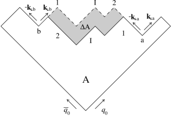
Fig. 1.: The decay of a Lund Model string spanning the space–time area $A$. The particles $1$ and $2$ are identical bosons and the particle(s) produced in between them is denoted by $I$. The two ways to produce the state are shown.

The calculation of the weight function for $n$ identical bosons contains $n!-1$ terms and it is therefore from a computational point of view of exponential-type. We have in reference[1] introduced approximate methods so that it becomes of power-type instead and we refer for details to this work.

We have seen that the transverse and longitudinal components of the particles momenta stem from different generation mechanisms. This is clearly manifested in the weight in equation7 where they give different contributions. In the following we will therefore in some detail analyse the impact of this difference on the transverse and longitudinal correlation lengths, as implemented in the model.

In order to understand the properties of the weight in equation7 we again consider the simple case in figure1. The area difference of the two configurations depends upon the energy momentum vectors $p_{1},p_{2}$ and $p_{I}$ and can in a dimensionless and useful way be written as

$$\frac{\mathchar 257\relax A}{2\kappa}=\delta p\delta x_{L}$$ (8)

where $\delta p=p_{2}-p_{1}$ and $\delta x_{L}=(\delta t;0,0,\delta z)$ is a reasonable estimate of the space-time difference, along the surface area, between the production points of the two identical bosons.

To preserve the transverse momenta of the particles in the state $(1,I,2)$ it is necessary to change the generated ${\bf k}_{\perp}$ at the two internal vertices around the state $I$ during the permutation, i.e. to change the Gaussian weights. Also in this case we may write a formula similar to equation8 for the transverse momentum change:

$$\frac{\mathchar 257\relax(\sum{\bf k}_{\perp j}^{2})}{2\kappa}=\delta{\bf p}_{\perp}\delta{\bf x}_{\perp}$$ (9)

where ${\delta{\bf p}}_{\perp}$ is the difference ${\bf p}_{\perp 2}-{\bf p}_{\perp 1}$ and $\delta{\bf x}_{\perp}=({\bf k}_{\perp b}-(-{\bf k}_{\perp a}))/\kappa$. The two neighbour vertices to the state $(1,I,2)$ ($(2,I,1)$) are denoted by $a$ and $b$ and ${\bf k}_{\perp b}+{\bf k}_{\perp a}$ corresponds to the state’s transverse momentum exchange to the outside. Therefore $\delta{\bf x}_{\perp}$ constitutes a possible estimate of the transverse distance between the production points of the pair.

For the general case when the permutation ${\cal P}^{\prime}$ is more than a two-particle exchange there are formulas similar to equations8 and 9.

It is evident from the considerations leading to equations8 and 9 that only particles with a finite longitudinal distance and small relative energy momenta will give significant contributions to the weights. We also note that we are in this way describing longitudinal correlation lengths along the color fields, inside which a given flavor combination is compensated. The corresponding transverse correlation length describes the tunneling (and in this model it provides a damping chaoticity).

The weight distribution we obtain is discussed in reference[1]. It is strongly centered around unity and we find negligible changes in the JETSET default observables (besides the correlation functions) by this extension of the Lund model.

3 Results

We have analysed two- and three-particle correlations in the Longitudinal Centre-of-Mass System (LCMS). For each pair (triplet) of particles the LCMS is the system in which the sum of the particles momentum components along the jet axis is zero. In the pair analysis we have used the kinematical variables

$$q_{\perp}=\sqrt{(p_{x2}-p_{x1})^{2}+(p_{y2}-p_{y1})^{2}}$$ (10)

$$q_{L}=|p_{z2}-p_{z1}|$$

and in the triplet analysis we have used

$$q_{\perp}=\sqrt{q_{\perp 12}^{2}+q_{\perp 13}^{2}+q_{\perp 23}^{2}}$$ (11)

$$q_{L}=\sqrt{q_{L12}^{2}+q_{L13}^{2}+q_{L23}^{2}}$$

where the jet axis is along the z-axis.

We have taken the ratio of the two-particle probability density of pions, $\rho_{2}$, with and without BE weights applied as the two-particle correlation function, $R_{2}$

$$R_{2}(p_{1},p_{2})=\frac{\rho_{2w}(p_{1},p_{2})}{\rho_{2}(p_{1},p_{2})}$$ (12)

and the resulting distribution is shown in figure2. It is clearly seen that it is not symmetric in $q_{L}$ and $q_{\perp}$ and in particular that the correlation length , as measured by the inverse of the width of the correlation function, is longer in the longitudinal than in the transverse direction. This difference remains for reasonable changes of the width in the transverse momentum generation. Using all the final pion pairs in the analysis results in in a small decrease in the transverse correlation length and of course a large decrease in the height for $q_{L}\simeq q_{\perp}\simeq 0$, while the longitudinal correlation length is rather unaffected.

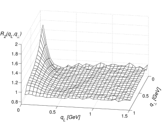
Fig. 2.: The two-particle correlation function $R_{2}(q_{L},q_{\perp})$ for charged pions. The sample consistes of particles which are either initially produced or stemming from short-lived resonances.

The total three-particle correlation function is in analogy with equation12

$$R_{3}^{{}^{\prime\prime}}(p_{1},p_{2},p_{3})=\frac{\rho_{3w}(p_{1},p_{2},p_{3})}{\rho_{3}(p_{1},p_{2},p_{3})}$$ (13)

To get the genuine three-particle correlation function, $R_{3}$, the consequences of having two-particle correlations in the model have to be subtracted from $R_{3}^{{}^{\prime\prime}}$. To this aim we have calculated the weight taking into account only configurations where pairs are exchanged, $w^{{}^{\prime}}$. In this way the three-particle correlations which only are a consequence of lower order correlations can be defined as

$$R_{3}^{{}^{\prime}}(p_{1},p_{2},p_{3})=\frac{\rho_{3w^{{}^{\prime}}}(p_{1},p_{2},p_{3})}{\rho_{3}(p_{1},p_{2},p_{3})}$$ (14)

The genuine three-particle correlation function, $R_{3}$, is then given by

$$R_{3}=R_{3}^{{}^{\prime\prime}}-R_{3}^{{}^{\prime}}+1$$ (15)

This way of getting the genuine correlations is not possible in an experimental situation, where one has to find other ways to get a $R_{3}^{{}^{\prime}}$ reference sample. We have suggested one possible option in reference[1].

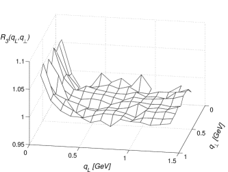
Fig. 3.: The genuine three-particle correlation function $R_{3}(q_{L},q_{\perp})$ for all final state charged pions.

The distribution $R_{3}$ is shown in figure3. The effect of the higher order terms is to pull the triplets closer in longitudinal direction while the transverse direction is rather unaffected. This suggests that the higher order terms are more sensitive to the longitudinal stretching of the string field.

References

-
[1]
B. Andersson and M. Ringnér,
LU TP 97-07 and hep-ph/9704383 (1997)
(accepted for publication in Nucl.Phys.B) -
[2]
B. Andersson and W. Hofmann,
Physics Letters B199 (1986), 364 -
[3]
B. Andersson et al.,
Phys. Rep. 97 (1983), 31 -
[4]
T. Sjöstrand,
Comp. Phys. Comm. 82 (1994), 74