ELECTROWEAK PRECISION OBSERVABLES IN THE MSSM AND GLOBAL ANALYSES OF PRECISION DATA

Abstract

The calculation of electroweak precision observables in the MSSM is reviewed. The description of the data of 1997 and results of updated global fits are discussed in comparison with the Standard Model.

The calculation of electroweak precision observables in the MSSM is reviewed. The description of the 1997 data and the results of updated global fits are discussed in comparison with the Standard Model.

1 Introduction

Experiments have measured the electroweak observables of the $W$ and $Z$ bosons $\!{}^{{\bf?}}$ and the top quark $\!{}^{{\bf?}}$ with an impressive accuracy thus providing precision tests of the electroweak theory at a level which had never been reached before. The description of the current precision data by the minimal Standard Model is extaordinarily successful, with a few observed deviations of the order $\geq 2\sigma$. They lower the quality of the Standard Model fits, but they can be understood as fluctuations which are statistically normal.

Extensions of the Standard Model hence are essentially theoretically motivated. Among the supersymmetric extensions, the $R$-parity conserving minimal supersymmetric standard model (MSSM) with the minimal particle content plays a special role as the most predictive framework beyond the Standard Model. Besides introducing the superpartners for the standard particles, the Higgs sector has to be augmented by a second scalar doublet. The structure of the MSSM allows a similarly complete calculation of the electroweak precision observables as in the Standard Model in terms of one Higgs mass and the ratio $v_{2}/v_{1}$ of the Higgs vacua together with the set of SUSY soft breaking parameters fixing the chargino/neutralino and scalar fermion sectors. Besides the direct searches for SUSY particles, which as yet have not been successful $\!{}^{{\bf?}}$, the interest for indirect tests of the MSSM in terms of virtual effects from the non-standard particles has triggered a broad activity in calculating and investigating the supersymmetric quantum effects in the electroweak precision observables $\!{}^{{\bf?},{\bf?},{\bf?},{\bf?},{\bf?}}$. Complete one-loop calculations are available for the quantity $\Delta r$ in the $M_{W}$-$M_{Z}$ correlation $\!{}^{{\bf?}}$ and for the $Z$ boson observables $\!{}^{{\bf?},{\bf?}}$ and have recently been improved by the supersymmetric QCD corrections to the $\rho$-parameter at the two-loop level $\!{}^{{\bf?}}$.

2 MSSM entries

The quantum contributions to the electroweak precision observables contain, besides the standard input, the following entries:

Higgs sector: The scalar sector of the MSSM, consisting of three neutral particles $h^{0},\,H^{0},\,A^{0}$ and a pair of charged bosons $H^{\pm}$, is completely determined by the value of $\tan\beta=v_{2}/v_{1}$ and the pseudoscalar mass $M_{A}$, together with the radiative corrections. The latter ones can be easily taken into account by means of the effective potential approximation with the leading terms $\sim m_{t}^{4}$, including mixing in the scalar top system $\!{}^{{\bf?}}$. In this way, the coupling constants of the various Higgs particles to gauge bosons and fermions can be taken from $\!{}^{{\bf?}}$ substituting only the scalar mixing angle $\alpha$ by the improved effective mixing angle which is obtained from the diagonalization of the scalar mass matrix. The mass of the light $h^{0}$ is constrained to $<\,130$ GeV when the dominant two-loop corrections are included $\!{}^{{\bf?}}$.

Chargino/Neutralino sector: The chargino (neutralino) masses and the mixing angles in the gaugino couplings are calculated from soft breaking parameters $M_{1}$, $M_{2}$ and $\mu$ in the chargino (neutralino) mass matrix $\!{}^{{\bf?}}$. For practical calculations, the GUT relation $M_{1}=5/3\tan^{2}\theta_{W}\,M_{2}$ is conventionally assumed.

The chargino $2\times 2$ mass matrix is given by

$$\cal{M}_{\rm\tilde{\chi}^{\pm}}\rm=\left(\begin{array}[]{l l}M_{2}&\quad M_{W}\sqrt{2}\sin\beta\\ M_{W}\sqrt{2}\cos\beta&\quad-\mu\\ \end{array}\right)\ ,$$ (1)

with the SUSY soft breaking parameters $\mu$ and $M_{2}$ in the diagonal matrix elements. The physical chargino mass states $\tilde{\chi}^{\pm}_{i}$ are the rotated wino and charged Higgsino states:

$$\tilde{\chi}^{+}_{i} = V_{ij}\psi^{+}_{j}$$

$$\tilde{\chi}^{-}_{i} = U_{ij}\psi^{-}_{j}\ ;\ i,j=1,2\ .$$ (2)

$V_{ij}$ and $U_{ij}$ are unitary chargino mixing matrices obtained from the diagonalization of the mass matrix Eq. (1):

$$\rm U^{*}\cal{M}_{\rm\tilde{\chi}^{\pm}}\rm V^{-1}=diag(m_{\tilde{\chi}^{\pm}_{1}},m_{\tilde{\chi}^{\pm}_{2}})\ .$$ (3)

The neutralino $4\times 4$ mass matrix $\cal{M}_{\rm\tilde{\chi}^{0}}$ can be written as:

$$\left(\begin{array}[]{cccc}M_{1}&0&-M_{Z}\sin\theta_{W}\cos\beta&M_{Z}\sin\theta_{W}\sin\beta\\ 0&M_{2}&M_{Z}\cos\theta_{W}\cos\beta&-M_{Z}\cos\theta_{W}\sin\beta\\ -M_{Z}\sin\theta_{W}\cos\beta&M_{Z}\cos\theta_{W}\cos\beta&0&\mu\\ M_{Z}\sin\theta_{W}\sin\beta&-M_{Z}\cos\theta_{W}\sin\beta&\mu&0\\ \end{array}\right)$$ (4)

where the diagonalization can be obtained by the unitary matrix $N_{ij}$:

$$\rm N^{*}\cal{M}_{\rm\tilde{\chi}^{0}}\rm N^{-1}=diag(m_{\tilde{\chi}_{i}^{0}})\ .$$ (5)

The elements $U_{ij}$, $V_{ij}$, $N_{ij}$ of the diagonalization matrices enter the couplings of the charginos, neutralinos and sfermions to fermions and gauge bosons, as explicitly given in ref. $\!{}^{{\bf?}}$. Note that the sign convention on the parameter $\mu$ is opposite to that of ref. $\!{}^{{\bf?}}$.

Sfermion sector: The physical masses of squarks and sleptons are given by the eigenvalues of the $2\times 2$ mass matrix:           $\cal M_{\rm\tilde{f}}^{\rm 2}\quad=$

$$\left(\begin{array}[]{ll}M_{\tilde{Q}_{L}}^{2}+m_{f}^{2}+M_{Z}^{2}(I_{3}^{f}-Q_{f}s_{W}^{2})\cos 2\beta&\quad m_{f}(A_{f}+\mu\{\cot\beta,\tan\beta\})\\ m_{f}(A_{f}+\mu\{\cot\beta,\tan\beta\})&\quad M_{\{\tilde{U},\tilde{D}\}_{R}}^{2}+m_{f}^{2}+M_{Z}^{2}Q_{f}s_{W}^{2}\cos 2\beta\end{array}\right)\ ,$$ (6)

with SUSY soft breaking parameters $M_{\tilde{Q}_{L}}$, $M_{\tilde{U}_{R}}$, $M_{\tilde{D}_{R}}$, $A_{f}$, and $\mu$. It is convenient to use the following notation for the off-diagonal entries in Eq. (6):

$$M_{f}^{LR}=A_{f}+\mu\{\cot\beta,\tan\beta\}\ .$$ (7)

Scalar neutrinos appear only as left-handed mass eigenstates. Up and down type sfermions in (6) are distinguished by setting f=u,d and the corresponding $\{u,d\}$ entries in the parenthesis. Since the non-diagonal terms are proportional to $m_{f}$, it seems natural to assume unmixed sfermions for the lepton and quark case except for the scalar top sector. The $\tilde{t}$ mass matrix is diagonalized by a rotation matrix with a mixing angle $\theta_{\tilde{t}}$. Instead of $M_{\tilde{Q}_{L}}$, $M_{\tilde{t}_{R}}$, $M_{\tilde{b}_{R}}$, $M_{t}^{LR}$ for the $\tilde{b}$, $\tilde{t}$ system ($Q=t,b$) the physical squark masses $m_{\tilde{b}_{L}},m_{\tilde{b}_{R}}$, $m_{\tilde{t}_{2}}$ can be used together with $M_{t}^{LR}$ or, alternatively, the stop mixing angle $\theta_{\tilde{t}}$. For simplicity one may assume $m_{\tilde{b}_{L}}=m_{\tilde{b}_{R}}$, and $\tilde{u}$, $\tilde{d}$, $\tilde{c}$, $\tilde{s}$ to have masses equal to the $\tilde{b}$ squark mass. The labels for the $\tilde{t}$ mass eigenstates are chosen in such a way that one gets $\tilde{t}_{1}=\tilde{t}_{L},\;\tilde{t}_{2}=\tilde{t}_{R}$ for the case of zero mixing.

3 Precision observables

3.1 The $\rho$-parameter

A possible mass splitting between the left-handed components of the $\tilde{b}$ and $\tilde{t}$ system yields a contribution to the $\rho$-parameter $\rho=1+\Delta\rho$ in terms of (neglecting left-right mixing in the $\tilde{b}$ sector)

$$\Delta\rho_{\tilde{t}\tilde{b}} = \frac{3G_{\mu}}{8\pi^{2}\sqrt{2}}\,\left[\cos^{2}\theta_{\tilde{t}}\;F_{0}(m_{\tilde{t}_{1}}^{2},m_{\tilde{b}_{L}}^{2})+\sin^{2}\theta_{\tilde{t}}\;F_{0}(m_{\tilde{t}_{2}}^{2},m_{\tilde{b}_{L}}^{2})\right.$$

$$\left.-\sin^{2}\theta_{\tilde{t}}\cos^{2}\theta_{\tilde{t}}\;F_{0}(m_{\tilde{t}_{1}}^{2},m_{\tilde{t}_{2}}^{2})\right]$$

$${\rm with} F_{0}(x,y)=x+y-\frac{2xy}{x-y}\log\frac{x}{y}$$ (8)

Examples for $\Delta\rho$ from the squark loops of the third generation, which can become remarkably large, are displayed in Figure 1. Recently the 2-loop $\alpha_{s}$ corrections have been computed $\!{}^{{\bf?},{\bf?}}$ which can amount to a sizeable fraction of the 1-loop $\Delta\rho_{\tilde{b}\tilde{t}}$. As a universal loop contribution, $\Delta\rho_{\tilde{t}\tilde{b}}$ enters the quantity $\Delta r$ and the $Z$ boson couplings through the relations (9) and (3.3) and is thus significantly constrained by the data on $M_{W}$ and the leptonic $Z$ widths.

Figure 1: $\Delta\rho_{\tilde{t}\tilde{b}}$ for $\tan\beta=1.6$. $M_{\tilde{t}_{L}}/M_{\tilde{t}_{R}}=1000/300$ (dotted), 300/1000 (solid)

3.2 The vector boson masses

The correlation between the masses $M_{W},M_{Z}$ of the vector bosons in terms of the Fermi constant $G_{\mu}$ is given by

$$\frac{G_{\mu}}{\sqrt{2}} = \frac{\pi\alpha}{2s_{W}^{2}M_{W}^{2}}\cdot\frac{1}{1-\Delta r}$$ (9)

$$= \frac{\pi\alpha}{2s_{W}^{2}M_{W}^{2}}\cdot\frac{1}{(1-\Delta\alpha)\cdot(1+\frac{c_{W}^{2}}{s_{W}^{2}}\Delta\rho)\,-\,(\Delta r)_{\rm rem}}$$

$${\rm with}\quad s_{W}^{2} = 1-\frac{M_{W}^{2}}{M_{Z}^{2}}\,.$$

Therein, $\Delta\alpha=0.0595\pm 0.0007$ $\!{}^{{\bf?}}$ is the QED vacuum polarization of the photon from the light fermions, $\Delta\rho$ is the irreducible quantum contribution to the $\rho$-parameter, and $(\Delta r)_{\rm rem}$ contains the residual loop terms. Complete 1-loop calculations for the quantity $\Delta r$ have been performed in ref’s $\!{}^{{\bf?}}$. Besides the higher order contributions beyond 1-loop from the Standard Model (see $\!{}^{{\bf?}}$ for more information and references), the SUSY-QCD 2-loop terms to $\Delta\rho$ are meanwhile available, as mentioned above in Section 3.1, as well as the complete 2-loop gluonic QCD corrections to the squark loop contributions to $\Delta r$ $\!{}^{{\bf?}}$. The SUSY QCD corrections to $\Delta r$ are well approximated by the SUSY QCD corrections to $\Delta\rho$. The 2-loop terms correspond to a shift in the $W$ mass of 10-20 MeV for not too heavy SUSY partners of the quarks and are thus of phenomenological importance.

By Eq. (9) the value for $M_{W}$ is fixed when $M_{Z}$ is taken as input and the MSSM model parameters have been chosen. Figure 2 displays the range of predictions for $M_{W}$ in the Standard Model (SM) and in the MSSM. Thereby it is assumed that no direct discovery has been made at LEP2 for constraining the model parameters. As one can see, precise determinations of $M_{W}$ and $m_{t}$ can become decisive for the separation between the models. The present world average $\!{}^{{\bf?}}$ $M_{W}=80.43\pm 0.08$ GeV together with $\!{}^{{\bf?}}$ $m_{t}=175.6\pm 5.5$ GeV shows a slight, but not significant, preference for the MSSM.

Figure 2: The $W$ mass range in the Standard Model (—–) and the MSSM (- - -). Bounds are from the non-observation of Higgs bosons and SUSY particles at LEP2.

3.3 $Z$ boson observables

With $M_{Z}$ as a precise input parameter, the predictions for the partial widths as well as for the asymmetries can conveniently be calculated in terms of effective neutral current coupling constants for the various fermions entering the neutral current vertex as follows:

$$J_{\nu}^{\rm NC} = g_{V}^{f}\,\gamma_{\nu}-g_{A}^{f}\,\gamma_{\nu}\gamma_{5}$$ (10)

$$= \left(\rho_{f}\right)^{1/2}\left[(I_{3}^{f}-2Q_{f}\,s_{f}^{2})\gamma_{\nu}-I_{3}^{f}\gamma_{\nu}\gamma_{5}\right]$$

with form factors $\rho_{f}$ for the overall normalization and with the effective mixing angles $s_{f}^{2}=\sin^{2}\theta_{f}$ for the corresponding fermions. The leading universal terms associated with the $\rho$-parameter enter the $Z$ boson couplings through

$$\rho_{f} = \frac{1}{1-\Delta\rho}+\cdots$$

$$s_{f}^{2} = s_{W}^{2}+c_{W}^{2}\,\Delta\rho+\cdots$$ (11)

Large non-universal contributions from the Higgs and the genuine SUSY particle sector are possible especially for the $b$-quark couplings.

Asymmetries and mixing angles:

The effective mixing angles are of particular interest since they determine the on-resonance asymmetries via the combinations

$$A_{f}=\frac{2g_{V}^{f}g_{A}^{f}}{(g_{V}^{f})^{2}+(g_{A}^{f})^{2}}\,.$$ (12)

Measurements of the asymmetries hence are measurements of the ratios

$$g_{V}^{f}/g_{A}^{f}=1-2Q_{f}s_{f}^{2}$$ (13)

or of the effective mixing angles $s^{2}_{f}$.

The measurable quantities are:

$-$ the forward-backward asymmetries in $e^{+}e^{-}\rightarrow f\bar{f}$:

$$A_{\rm FB}^{f}=\frac{3}{4}A_{e}\cdot A_{f}$$

$-$ the left-right asymmetry:

$$A_{\rm LR}=A_{e}$$

$-$ the $\tau$ polarization in $e^{+}e^{-}\rightarrow\tau^{+}\tau^{-}$ :

$$P_{\tau}=A_{\tau}\,.$$

It is interesting to note that the non-standard loop contributions to the leptonic mixing angle $s_{e}^{2}$ diminish the Standard Model value. A small experimental value, as observed in $A_{\rm LR}$, could therefore be accomodated in the MSSM also for a relatively high top mass.

$Z$ widths and cross sections:

The total $Z$ width $\Gamma_{Z}$ can be calculated essentially as the sum over the fermionic partial decay widths:

$$\Gamma_{Z}=\sum_{f}\,\Gamma_{f},\;\;\;\;\Gamma_{f}=\Gamma(Z\rightarrow f\bar{f})\,.$$ (14)

The peak cross sections for $e^{+}e^{-}\rightarrow f\bar{f}$ (had) are determined by

$$\sigma_{0}^{f}=\frac{12\pi}{M_{Z}^{2}}\frac{\Gamma_{e}\Gamma_{f}}{\Gamma_{Z}^{2}},\quad\sigma_{0}^{\rm had}=\frac{12\pi}{M_{Z}^{2}}\frac{\Gamma_{e}\Gamma_{\rm had}}{\Gamma_{Z}^{2}}\,.$$ (15)

The partial widths, expressed in terms of the effective coupling constants, read up to 2nd order in the fermion masses:

$$\Gamma_{f} = \Gamma_{0}\,\left((g_{V}^{f})^{2}+(g_{A}^{f})^{2}(1-\frac{6m_{f}^{2}}{M_{Z}^{2}})\right)\cdot(1+Q_{f}^{2}\,\frac{3\alpha}{4\pi})+\Delta\Gamma^{f}_{QCD}$$

with

$$\Gamma_{0}\,=\,N_{C}^{f}\,\frac{\sqrt{2}G_{\mu}M_{Z}^{3}}{12\pi},\;\;\;\;N_{C}^{f}=1\mbox{ (leptons)},\;\;=3\mbox{ (quarks)}.$$

and the QCD corrections $\Delta\Gamma^{f}_{QCD}$ for quark final states, both from standard (see $\!{}^{{\bf?}}$ for references) and SUSY QCD. The gluino contribution, however, is very small.

Of particular interest is the quantity

$$R_{\rm b}=\frac{\Gamma_{\rm b}}{\Gamma_{\rm had}}$$ (16)

which in the Standard Model is most sensitive to the mass of the top quark. As already known for quite some time $\!{}^{{\bf?}}$, light non-standard Higgs bosons for large $\tan\beta$ as well as light stop and charginos influence the $b$-quark couplings remarkably and predict larger values for the ratio $R_{b}$ in the MSSM $\!{}^{{\bf?},{\bf?}}$ (see figures 3, 4).

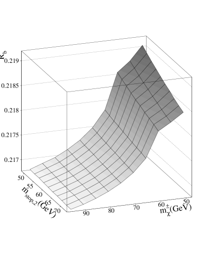
Figure 3: $R_{b}$ in the light stop-chargino plane. $\tan\beta=1.6$. $\!{}^{{\bf?}}$

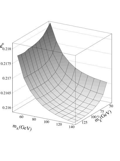
Figure 4: $R_{b}$ in the pseudoscalar Higgs - chargino plane. $\tan\beta=34$. $\!{}^{{\bf?}}$

4 MSSM global fits to precision data

For obtaining the optimized SUSY parameter set a global fit to all the electroweak precision data, including the top mass measurement, has to be performed. Two strategies can be persued: (i) the parameters of the MSSM are further restricted by specific model assumptions like unification scenarios, or (ii) the MSSM parameters are considered as free quantitites chosen in the optimal way for improving the observed deficiencies of the Standard Model in describing the data. (ii) has been applied in $\!{}^{{\bf?}}$, recently updated by Schwickerath $\!{}^{{\bf?}}$. In the past, the experimental value of $R_{\rm b}$ was $3.7\sigma$ away from the Standard Model predictions and could be accomodated much better in MSSM scenarios with light stop and charginos and/or light scalar amd pseudoscalar Higgs bosons. In the meantime, $R_{\rm b}$ has decreased and is now much closer to the Standard Model value. Instead, $A_{\rm FB}^{\rm b}$ shows a $2\sigma$ deviation between data and Standard Model prediction $\!{}^{{\bf?}}$.

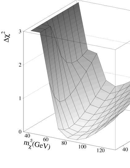
Figure 5: $\Delta\chi^{2}$ for $\tan\beta=1.5$. No limits for supersymmetric particle masses are imposed (from $\!{}^{{\bf?}}$ updated in $\!{}^{{\bf?}}$ )

In order to obtain the best MSSM fits the electroweak precision data are taken into account together with the error correlations $\!{}^{{\bf?}}$, and the measurement of the branching ratio $R_{b\rightarrow s\gamma}={\rm BR}(B\rightarrow X_{s}\gamma)$ by CLEO and ALEPH $\!{}^{{\bf?}}$ with the combined value $(2.55\pm 0.61)\cdot 10^{-4}$. The $b\rightarrow s\gamma$ rate becomes too small if $\tan\beta$ is near one. For $\tan\beta=1.6$ and 35, MSSM solutions can be found which are compatible with $R_{b\rightarrow s\gamma}$ and the electroweak precision data. For the MSSM calculation of $R_{b\rightarrow s\gamma}$, the results of $\!{}^{{\bf?}}$ are used with a chosen renormalization scale of $\mu=0.65m_{b}$.

For reducing the large number of parameters, the simplifying assumptions described in Section 2 are applied. As a common squark mass scale the value $M_{\tilde{Q}}=1$ TeV is chosen; $M_{\tilde{t}_{R}}$ and the stop mixing angle $\theta_{\tilde{t}}$ are kept free to allow for a light stop state $\tilde{t}_{2}$. This state has to be predominatly right-handed to avoid deteriorations of the $\rho$-parameter according to Eq. (3.1). In the slepton sector, common masses of 0.5 TeV are assumed for both left and right-handed components neglecting left-right mixing. The fits are insensitive to the detailed values of the heavy particles. Figure 5 shows the increase of the $\chi^{2}$ of the fit $\!{}^{{\bf?}}$ in the light stop-chargino plane ($\Delta\chi^{2}=\chi^{2}-\chi^{2}_{\rm min}$). In each point, the parameters $m_{t},\alpha_{s},\theta_{\tilde{t}},M_{2}$ are optimized.

Table 1: Fitted parameters and mass spectrum for the best low and high $\tan\beta$ fits $\!{}^{{\bf?}}$, updated from $\!{}^{{\bf?}}$. Parameter values in brackets are not fitted, but fixed to the given value during the fit.

	$\tan\beta$=1.5	$\tan\beta$=35
$\chi^{2}$/d.o.f.	15.0/13	15.8/13
prob.	31%	26%
fitted parameters
$\alpha_{s}(M_{Z}^{2})$	0.1161	0.1196
$m_{t}$ [GeV]	174.0	174.3
$M_{2}$ [GeV]	68	(1500)
$\mu$ [GeV]	79	92
$m_{A}$ [GeV]	(1500)	60
$m_{\tilde{t}_{2}}$ [GeV]	80	81
$\theta_{\tilde{t}}$	-0.139	0.0126
mass spectrum
$\tilde{\chi_{1}}^{\pm}$,$\tilde{\chi_{2}}^{\pm}$ [GeV]	89, 126	92, 1504
$\tilde{\chi_{1}}^{0}$,$\tilde{\chi_{2}}^{0}$[GeV]	38,70	89,96
$\tilde{\chi_{3}}^{0}$,$\tilde{\chi_{4}}^{0}$[GeV]	115,123	716,1504
$m_{\tilde{t}_{1}}$ [GeV]	1023	1012
$M_{h},M_{H}$ [GeV]	98,1503	60,103
$M_{H^{\pm}}$ [GeV]	1502	124
$M_{W}$ [GeV]	80.42	80.43

Constraints from direct searches for SUSY particles $\!{}^{{\bf?}}$ can be taken into account with the help of a penalty function (see $\!{}^{{\bf?}}$): $M_{A}>50$ GeV, $M_{h}>60$ GeV, $m_{\tilde{\chi}^{+}}>85$ GeV, $m_{\tilde{t}_{2}}>80$ GeV. With these constraints the best fit results for a low and high $\tan\beta$ scenario are listed in Table 1. The values of the strong coupling constant $\alpha_{s}$ is close to the best fit value of the Standard Model $\!{}^{{\bf?}}$ $\alpha_{s}({\rm SM})=0.120\pm 0.003$. For the low $\tan\beta$ scenario $\alpha_{s}$ is slightly lower; this is due to the positive loop contribution to the partial $Z$ width $\Gamma_{\rm b}$, which is less pronounced in the high $\tan\beta$ scenario because of the constraints to the Higgs masses. The particle spectrum for the best fits suggests that some SUSY particles could be within reach of LEP 2; the $\chi^{2}$ in the region of the best low $\tan\beta$ fit, however, increases only slowly for increasing chargino masses. Within the high $\tan\beta$ scenario both neutral $h^{0},A^{0}$ bosons are light and have practically the same mass. This scenario can be excluded if no Higgs bosons will be found at LEP 2.

Figure 6: Experimental data normalized to the best fit results in the SM and MSSM for low $\tan\beta$, with experimental error bars (updated from $\!{}^{{\bf?}}$ in $\!{}^{{\bf?}}$).

Figure 7: Experimental data normalized to the best fit results in the SM and MSSM for high $\tan\beta$, with experimental error bars (updated from $\!{}^{{\bf?}}$ in $\!{}^{{\bf?}}$).

A direct comparison to the Standard Model fit is shown in Figure 6 for $\tan\beta=1.6$. A very similar plot is obtained for $\tan\beta=35$ displayed in Figure 7. The present small difference between the experimental and the SM value of $R_{\rm b}$ can be completely removed in the MSSM for the low $\tan\beta$. Other quantities are practically unchanged; in particular, the difference between data and theory observed in $A_{\rm FB}^{\rm b}$ cannot be significantly diminished. The $\chi^{2}$ of the MSSM fits are lower than in the Standard Model, but due to the larger number of parameters the probability in the MSSM is not higher than in the Standard Model (31%); for high $\tan\beta$ the probability is even lower. (The small difference to the SM result of the LEP Electroweak Working Group is due to the inclusion of $R_{b\rightarrow s\gamma}$ in our fit.) This means that the MSSM yields an equally good description of the data as the minimal Standard Model and is thus competitive, but it does not appear as superior.

5 Conclusions

The supersymmetric extension of the Standard Model realized in terms of the MSSM permits a similar complete calculation of the electroweak precision observables as in the Standard Model. The version with all SUSY particles and the $A^{0},H^{0},H^{\pm}$ Higgs bosons heavy is equivalent to the Standard Model with a light Higgs around 120 GeV. The possibility of having some of the non-standard particles light, in the mass range around 100 GeV, opens the option to remove some of the observed deviations between data and theory, like in $R_{\rm b}$. The overall $\chi^{2}$ of a global fit is therefore slightly lower than in a corresponding Standard Model fit; the larger number of parameters, however, reduce the $\chi^{2}$ per degree of freedom and thus the probability of the MSSM to that of the Standard Model. The MSSM thus yields an equally good description of the precision data as the Standard Model. It is always possible to worsen the fits by inappropriate choices of the model parameters, which can be used to exclude certain regions of the parameter space, as done recently in $\!{}^{{\bf?}}$. The $W$ mass predicted by the MSSM is always higher than in the Standard Model; present data show a slightly better agreement with the MSSM. From the increasing experimental accuracy for $M_{W}$ and $m_{t}$ in the future one hence expects a very important probe for both the Standard Model and the MSSM.

References

References

-
[1]
The LEP Collaborations ALEPH, DELPHI, L3, OPAL, the LEP Electroweak
Working Group and the SLD Heavy Flavor Working Group,
CERN-PPE/96-183 (1996); for the update see:
J. Timmermans, Proceedings of the XVIII International Symposium on Lepton-Photon Interactions, Hamburg 1997;
D. Ward, Proceedings of the International Europhysics Conference on High Energy Physics, Jerusalem 1997 - [2] P. Giromini, Proceedings of the XVIII International Symposium on Lepton-Photon Interactions, Hamburg 1997
- [3] P. Janot, Proceedings of the International Europhysics Conference on High Energy Physics, Jerusalem 1997
-
[4]
A. Denner, R. Guth, W. Hollik, J.H. Kühn,
Z. Phys. C 51 (1991) 695;
J. Rosiek, Phys. Lett. B 252 (1990) 135;
M. Boulware, D. Finnell, Phys. Rev. D 44 (1991) 2054 -
[5]
G. Altarelli, R. Barbieri, F. Caravaglios,
Phys. Lett. B 314 (1993) 357;
C.S. Lee, B.Q. Hu, J.H. Yang, Z.Y. Fang, J. Phys. G 19 (1993) 13;
Q. Hu, J.M. Yang, C.S. Li, Comm. Theor. Phys. 20 (1993) 213;
J.D. Wells, C. Kolda, G.L. Kane, Phys. Lett. B 338 (1994) 219;
G.L. Kane, R.G. Stuart, J.D. Wells, Phys. Lett. B 354 (1995) 350;
M. Drees et al., Phys. Rev. D 54 (1996) 5598;
J. Ellis, G. Fogli. E. Lisi, Phys. Lett. B 389 (1996) 321 -
[6]
P. Chankowski, A. Dabelstein, W. Hollik, W. Mösle,
S. Pokorski, J. Rosiek, Nucl. Phys. B 417 (1994) 101;
D. Garcia, J. Solà, Mod. Phys. Lett. A 9 (1994) 211 -
[7]
D. Garcia, R. Jiménez, J. Solà,
Phys. Lett. B 347 (1995) 309; B 347 (1995) 321;
D. Garcia, J. Solà, Phys. Lett. B 357 (1995) 349;
A. Dabelstein, W. Hollik, W. Mösle, in Perspectives for Electroweak Interactions in Collisions, Ringberg Castle 1995, Ed. B.A. Kniehl, World Scientific 1995 (p. 345);
P. Chankowski, S. Pokorski, Nucl. Phys. B 475 (1996) 3 - [8] W. de Boer, A. Dabelstein, W. Hollik, W. Mösle, U. Schwickerath, Z. Phys. C 75 (1997) 627
- [9] A. Djouadi, P. Gambino, S. Heinemeyer, W. Hollik, C. Jünger, G. Weiglein, Phys. Rev. Lett. 78 (1997) 3626; – hep-ph/9710438
- [10] J. Ellis, G. Ridolfi and F. Zwirner, Phys. Lett. B 257 (1991) 83
-
[11]
H. P. Nilles, Phys. Rep. 110 (1984) 1;
H. E. Haber, G. Kane, Phys. Rep. 117 (1985) 75;
J. F. Gunion, H. E. Haber, Nucl. Phys. B 272 (1986) 1;
Nucl. Phys. B 402 (1993) 567;
J. F. Gunion, H. E. Haber, G. Kane, S. Dawson: The Higgs Hunter’s Guide, Addison-Wesley 1990. -
[12]
R. Hempfling, A. Hoang, Phys. Lett. B 331 (1994) 99;
M Carena, M. Quiros, C. Wagner, Nucl. Phys. B 461 (1996) 407 - [13] S. Heinemeyer, 2-Loop Calculations in the MSSM, these Proceedings
-
[14]
S. Eidelman, F. Jegerlehner,
Z. Phys. C 67 (1995) 585;
H. Burkhardt, B. Pietrzyk, Phys. Lett. B 356 (1995) 398 - [15] W. Hollik, Review Status of the Standard Model, these Proceedings
- [16] U. Schwickerath, Proceedings of the XVI International Workshop on Weak Interactions and Neutrinos (WIN’97), Capri 1997
- [17] CLEO-Collaboration, R. Ammar et al., Phys. Rev. Lett. 74 (1995) 2885; M. Feindt, Proceedings of the International Europhysics Conference on High Energy Physics, Jerusalem, August 1997 (to appear)
-
[18]
R. Barbieri, G. Giudice, Phys. Lett.
B 309 (1993) 86;
R. Garisto, J.N. Ng, Phys. Lett. B 315 (1993) 372;
S. Bertolini, F. Borzumati, A.Masiero, G. Ridolfi, Nucl. Phys. B 353 (1991) 591 and references therein;
N. Oshimo, Nucl. Phys. B 404 (1993) 20;
S. Bertolini, F. Vissani, Z. Phys. C 67 (1995) 513, 1995 - [19] D.M. Pierce, J. Erler, hep-ph/9708374