MPI/PhT/97–79
hep-ph/9711465
November 1997

Higher Order Corrections to the Hadronic Higgs Decay

Abstract

A Higgs boson in the intermediate mass range is considered. An effective Lagrangian approach is used in order to evaluate the top-induced QCD corrections of order $\alpha_{s}^{3}$ to the decay into light quarks and ${\cal O}(\alpha_{s}^{4})$ corrections to the gluonic decay mode. The connection to the decoupling relations for $\alpha_{s}$ and the light quark masses is discussed.

The Higgs boson is the only still missing particle in the standard model. Currently only lower bounds of roughly $70$ GeV have been obtained from the failure of finding the Higgs boson at the Large Electron-Positron Collider (LEP) at CERN. A global fit to the precision date also prefers a Higgs mass in the so-called intermediate mass range with $M_{H}\;\hbox to0.0pt{\lower 3.5pt\hbox{$\mathchar 0\relax\sim$}\hss}\raise 1.0pt\hbox{$<$}\;2M_{W}$. In this contribution we will concentrate on such a Higgs boson. The dominant decay mode is then the one into bottom quarks. In the “massless” theory corrections are known up to ${\cal O}(\alpha_{s}^{3})$ [1]. In this contribution we will discuss the top-induced correction terms of the same order [2].

A second very interesting decay mode of a Higgs boson in the intermediate mass range is the decay into gluons. The lowest order process is mediated by a quark loop. It is interesting to note that in the limit where the internal quark mass is much larger than $M_{H}$ the amplitude gets independent of the quark mass. Therefore this process counts the number of heavy quarks. In contrast to the electroweak $\rho$ parameter [3], the $ggH$ coupling is also sensitive to quark isodoublets if they are mass-degenerate. The first order QCD corrections to the triangle diagram where a top quark is running around are known since long [4, 5, 6]. It turned out that the order $\alpha_{s}$ corrections amount to approximately $70$ %. These large corrections were a strong motivation to evaluate the next term in the expansion in $\alpha_{s}$ [7]. Note that the $ggH$ coupling also appears as a building block in the process $gg\to H$ which is the dominant production mechanism at LHC.

As the top quark is much heavier than all other mass scales involved in the processes under consideration it makes sense to construct in a first step an effective Lagrangian. We start with the bare Yukawa Lagrangian,

$${\cal L}_{Y}=-\frac{H^{0}}{v^{0}}\left(\sum_{q}m_{q}^{0}\bar{q}^{0}q^{0}+m_{t}^{0}\bar{t}^{0}t^{0}\right){},$$ (1)

where $v$ is the Higgs vacuum-expectation value and the superscript 0 labels bare quantities. Assuming that the Higgs boson mass, $M_{H}$, is less than the top quark mass, $m_{t}$, ${\cal L}_{Y}$ can be replaced by an effective Lagrangian produced by integrating out the top quark field. According to Refs. [4, 8] the resulting Lagrangian reads

$${\cal L}_{Y}^{\rm eff} = -\frac{H^{0}}{v^{0}}\left[C_{1}\left[O_{1}^{\prime}\right]+\sum_{q}C_{2}\left[O_{2q}^{\prime}\right]\right],$$ (2)

where $[O_{1}^{\prime}]$ and $[O_{2q}^{\prime}]$ are the renormalized counterparts of the bare operators

$$O_{1}^{\prime}\,\,=\,\,\left(G_{a\mu\nu}^{0\prime}\right)^{2}, O_{2q}^{\prime}\,\,=\,\,m_{q}^{0\prime}\bar{q}^{0\prime}q^{0\prime},$$

with $G_{a\mu\nu}^{0\prime}$ being the (bare) field strength tensor of the gluon. The primes mark the quantities defined in the effective $n_{f}=5$ QCD including only light quarks. All the dependence on the top quark gets localized in the coefficient functions $C_{1}$ and $C_{2}$.

The task to compute the decay rates essentially splits into two parts: $(i)$ The evaluation of the coefficient functions where the scale is given by the top quark mass, and $(ii)$ the computation of the imaginary part of the correlators formed by the operators $O_{1}^{\prime}$ and $O_{2q}^{\prime}$. There the particles inside the loops are massless and for the external momentum one has $q^{2}=M_{H}^{2}$.

The computation of the coefficient function $C_{1}$ has been performed in two different way. The first method considers the vertex diagrams where the Higgs boson couples the top quark and where two gluons are in the final state (see Fig. 1). In order to calculate $C_{1}$ these graphs have to be expanded in their two external momenta.

xxxxx

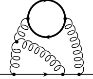
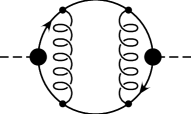
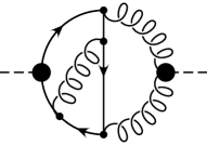
Figure 1: Typical Feynman diagrams contributing to $C_{1}$, $C_{2}$ and the three kind of correlators.

The second method is based on a low energy theorem (LET). We were able to derive the following simple formulae [9]:

$$C_{1}=-\frac{1}{2}\frac{\partial\ln\zeta_{g}^{2}}{\partial\ln m_{t}^{2}}, C_{2}=1+2\frac{\partial\ln\zeta_{m}}{\partial\ln m_{t}^{2}},$$ (3)

where $\zeta_{g}$ and $\zeta_{m}$ are the decoupling constants relating the strong coupling constant, $\alpha_{s}$, and the light quark masses, $m_{q}$, in the full and effective theory:

$$\alpha_{s}^{\prime}=\zeta_{g}\alpha_{s}, m_{q}^{\prime}=\zeta_{m}m_{q}.$$ (4)

$\zeta_{g}$ may be computed by considering the diagrams containing at least one top quark line of the gluon and ghost propagator and the gluon-ghost vertex with external momentum equal to zero. $\zeta_{m}$ is given by top-induced diagrams contributing to the fermion propagator (see Fig. 1). In [10, 9] $\zeta_{g}$ and $\zeta_{m}$ were evaluated up to the three-loop order. Eqs. (3) reduce the computation of $C_{1}$ and $C_{2}$ to the evaluation of essentially two-point functions with vanishing external momentum. With this method there are less diagrams to be considered which are in addition much simpler to evaluate. Another nice feature of Eqs. (3) is that because of the logarithmic derivative even the ${\cal O}(\alpha_{s}^{4})$ contributions to $C_{1}$ and $C_{2}$ can be evaluated if $\zeta_{g}$ and $\zeta_{m}$ are known up to ${\cal O}(\alpha_{s}^{3})$.

There are actually three types of correlators which have to be evaluated. In the bottom line of Fig. 1 some sample diagrams are pictured. The computation was performed with the program package MINCER [11].

The combination of the coefficient function and the imaginary part of the correlator $\langle\left[O_{1}^{\prime}\right]\left[O_{1}^{\prime}\right]\rangle$ immediately leads to the decay rate $\Gamma(H\to gg)$ ($\mu=M_{H}$):

$$\frac{\Gamma(H\to gg)}{\Gamma^{\rm Born}(H\to gg)}=$$ (5)

$$1+\frac{\alpha_{s}^{(5)}(M_{H})}{\pi}\left(\frac{95}{4}-\frac{7}{6}n_{l}\right)+\left(\frac{\alpha_{s}^{(5)}(M_{H})}{\pi}\right)^{2}\left[\frac{149533}{288}-\frac{363}{8}\zeta(2)\right.$$

$$\left.\mbox{}-\frac{495}{8}\zeta(3)-\frac{19}{8}\ln\frac{M_{t}^{2}}{M_{H}^{2}}+n_{l}\left(-\frac{4157}{72}+\frac{11}{2}\zeta(2)+\frac{5}{4}\zeta(3)-\frac{2}{3}\ln\frac{M_{t}^{2}}{M_{H}^{2}}\right)\right.$$

$$\left.\mbox{}+n_{l}^{2}\left(\frac{127}{108}-\frac{1}{6}\zeta(2)\right)\right]$$

$$\approx 1+17.917\,\frac{\alpha_{s}^{(5)}(M_{H})}{\pi}+\left(\frac{\alpha_{s}^{(5)}(M_{H})}{\pi}\right)^{2}\left(156.808-5.708\,\ln\frac{M_{t}^{2}}{M_{H}^{2}}\right),$$

with $\Gamma^{\rm Born}(H\to gg)=G_{F}M_{H}^{3}/36\pi\sqrt{2}\times(\alpha_{s}^{(5)}(M_{H})/\pi)^{2}$. Choosing $M_{t}=175$ GeV and $M_{H}=100$ GeV one arrives at:

$$\frac{\Gamma(H\to gg)}{\Gamma^{\rm Born}(H\to gg)} \approx 1+17.917\,\frac{\alpha_{s}^{(5)}(M_{H})}{\pi}+150.419\,\left(\frac{\alpha_{s}^{(5)}(M_{H})}{\pi}\right)^{2}$$ (6)

$$\approx 1+0.66+0.21.$$

We observe that the new ${\cal O}(\alpha_{s}^{2})$ term further increases the well-known ${\cal O}(\alpha_{s})$ enhancement by about one third. If we assume that this trend continues to ${\cal O}(\alpha_{s}^{3})$ and beyond, then Eq. (5) may already be regarded as a useful approximation to the full result. Inclusion of the new ${\cal O}(\alpha_{s}^{2})$ correction leads to an increase of the Higgs-boson hadronic width by an amount of order 1%.

The decay rate $\Gamma(H\to b\bar{b})$ can be cast into the form

$$\Gamma(H\to b\bar{b})=A_{b\bar{b}}\Bigg{\{}1+5.667\,a_{H}^{(5)}+29.147\,\left(a_{H}^{(5)}\right)^{2}+41.758\left(a_{H}^{(5)}\right)^{3}$$

$$\mbox{}+\left(a_{H}^{(5)}\right)^{2}\left[3.111-0.667\,L_{t}\right]+\left(a_{H}^{(5)}\right)^{3}\left[50.474-8.167\,L_{t}-1.278\,L_{t}^{2}\right]\Bigg{\}},$$

with $A_{b\bar{b}}=3G_{F}M_{H}m_{b}^{2}/4\pi\sqrt{2}$, $L_{t}=\ln M_{H}^{2}/M_{t}^{2}$ and $a_{H}^{(5)}=\alpha_{s}^{(5)}(M_{H})/\pi$. In Eq. ( MPI/PhT/97–79 hep-ph/9711465 November 1997 Higher Order Corrections to the Hadronic Higgs Decay) electromagnetic and electroweak corrections have been neglected. Also mass correction terms and second order QCD corrections which are suppressed by the top quark mass are not displayed. One observes from Eq. ( MPI/PhT/97–79 hep-ph/9711465 November 1997 Higher Order Corrections to the Hadronic Higgs Decay) that the top-induced corrections at ${\cal O}(\alpha_{s}^{3})$ are of the same order of magnitude than the “massless” corrections.

I would like to thank K.G. Chetyrkin and B.A. Kniehl for the fruitful collaboration on this subject.

References

- [1] K.G. Chetyrkin, Phys. Lett. B 390 (1997) 309.
- [2] K.G. Chetyrkin and M. Steinhauser, Phys. Lett. B 408 (1997) 320.
- [3] M. Veltman, Nucl. Phys. B 123, (1977) 89.
- [4] T. Inami, T. Kubota and Y. Okada, Z. Phys. C 18, (1983) 69.
- [5] S. Dawson, Nucl. Phys. B 359, (1991) 283; S. Dawson and R.P. Kauffman, Phys. Rev. Lett. 68, (1992) 2273; Phys. Rev. D 49, (1994) 2298; D. Graudenz, M. Spira and P.M. Zerwas, Phys. Rev. Lett. 70, (1993) 1372; M. Spira, A. Djouadi, D. Graudenz and P.M. Zerwas, Nucl. Phys. B 453, (1995) 17.
- [6] A. Djouadi, M. Spira and P.M. Zerwas, Phys. Lett. B 264, (1991) 440.
- [7] K.G. Chetyrkin, B.A. Kniehl and M. Steinhauser, Phys. Rev. Lett. 79 (1997) 353.
- [8] K.G. Chetyrkin, B.A. Kniehl and M. Steinhauser, Phys. Rev. Lett. 78 (1997) 594; Nucl. Phys. B 490 (1997) 19.
- [9] K.G. Chetyrkin, B.A. Kniehl and M. Steinhauser, hep-ph/9708255, Nucl. Phys. B (in press).
- [10] K.G. Chetyrkin, B.A. Kniehl and M. Steinhauser, Phys. Rev. Lett. 79 (1997) 2184.
- [11] S.A. Larin, F.V. Tkachev and J.A.M. Vermaseren, NIKHEF Report No. NIKHEF–H/91–18 (September 1991).