A Complete Order-$\alpha^{3}$ Calculation of the Cross Section for Polarized Compton Scattering^†

Abstract

The construction of a computer code to calculate the cross sections for the spin-polarized processes $e^{-}\gamma\to e^{-}\gamma,e^{-}\gamma\gamma,e^{-}e^{+}e^{-}$ to order-$\alpha^{3}$ is described. The code calculates cross sections for circularly-polarized initial-state photons and arbitrarily polarized initial-state electrons. The application of the code to the SLD Compton polarimeter indicates that the order-$\alpha^{3}$ corrections produce a fractional shift in the SLC polarization scale of $-$0.1% which is too small and of the wrong sign to account for the discrepancy in the Z-pole asymmetries measured by the SLD Collaboration and the LEP Collaborations.

Submitted to Physical Review D

^†This work was supported by Department of Energy contract DE-AC03-76SF00515

I Introduction

For some years, polarized Compton scattering, the scattering of circularly-polarized photons by spin-polarized electrons, has been used to measure the degree of polarization of one particle or the other. Circularly-polarized gamma-ray photons from nuclear decays have been polarization-analyzed by measuring the asymmetry in the rates of backscattering from magnetized iron foils (as the foil magnetization is reversed). Similarly, the polarization of electrons in high-energy storage rings and accelerators has been determined from scattering asymmetries of the accelerated beam with beams of optical laser photons. Until quite recently, all such measurements have made use of tree-level (order-$\alpha^{2}$) expressions for the polarized Compton scattering cross section.

Part of the reason for this has been the unavailability of a next-to-leading-order calculation that is packaged in an easily usable form. The first calculation of the order-$\alpha^{3}$ virtual and real-soft-photon corrections to unpolarized Compton scattering was published by Brown and Feynman in 1952 [1]. This calculation was not confirmed until 1972 when Tsai, DeRaad, and Milton (TDM) published the same corrections for the polarized case [2]. The TDM calculation, by itself, is sufficient to interpret the results of measurements involving longitudinally polarized electrons for which the presence of additional energetic photons in the final state can be excluded. This is often the case for measurements of gamma-rays that have been scattered from magnetized iron targets. However, accelerator-based polarimeters are often designed to measure transverse electron polarization and generally cannot distinguish between single-photon and multiple-photon final states. These shortcomings were addressed in 1987 by Góngora and Stuart (GS) who published the matrix elements for the hard-photon corrections in a spinor-product form that is suitable for numerical evaluation [3]. Their publication also includes spinor-product expressions for the matrix elements of six gauge-invariant tensors used by TDM to calculate their result. These expressions permit the application of the TDM virtual corrections to the case of general initial- and final-state electron spin directions. Finally, in 1989, the complete set of virtual, soft-photon, and hard-photon radiative corrections to polarized Compton scattering was calculated independently by Veltman [4]. Veltman’s paper describes her calculation qualitatively and presents a result in numerical form for two specific cases of an accelerator-based longitudinal polarimeter. Unfortunately, it does not include detailed expressions for the final result nor is the result checked against the TDM or GS calculations.

One of the specific cases discussed by Veltman, the case of a 50 GeV longitudinally-polarized electron colliding with a 2.34 eV photon, is quite close to that of the SLD Compton polarimeter (a 45.65 GeV longitudinally-polarized electron colliding with a 2.33 eV photon). This polarimeter is a key component in the measurement of the left-right $Z$-boson production asymmetry $A_{LR}^{0}$ which has been performed over several years by the SLD Collaboration [5]. At the current time, the measured value of $A_{LR}^{0}$ is approximately 8% larger than the value of the comparable quantity extracted from measurements of six different $Z$-pole asymmetries by the four LEP Collaborations [6]. Since the SLD and LEP measurements differ by approximately three standard deviations, the discrepancy is more likely to be due to systematic effects than to statistical fluctuations. One possible systematic effect is the absence of radiative corrections from the interpretation of the SLD polarimeter data. Veltman’s calculation implies that radiative corrections would shift the SLD polarization measurements by $-$0.1% of themselves which is far too small and of the wrong sign to account for the 8% discrepancy.

This paper describes a complete order-$\alpha^{3}$ calculation of polarized Compton Scattering. It was undertaken primarily to check the calculation of Veltman and to determine if radiative corrections to Compton scattering could be responsible for discrepancy between the LEP and SLD measurements of $Z$-pole asymmetries. A second goal was to develop a computer code which could applied to a variety of present and future experimental situations. The main ingredients of this code, the TDM and GS calculations, are sufficient for all present day experimental situations. However, it is likely that a very high energy linear electron-positron collider will be constructed somewhere in the world in the coming decade. Polarized beams are planned for all of the designs now under discussion. All of these projects incorporate Compton Scattering polarimeters into the optical designs of their final focusing systems. If these polarimeters use optical lasers, the $e^{-}\gamma$ center-of-mass energies will be above threshold for the production of final state $e^{+}e^{-}$ pairs. Since the process $e^{-}\gamma\to e^{-}e^{+}e^{-}$ occurs at order-$\alpha^{3}$, it must also be included in the computer code. A calculation of the matrix element for this process, based upon the techniques of Ref. [3], is described in Section II D.

The following sections of this paper describe the construction and operation of the Fortran-code COMRAD which calculates the order-$\alpha^{3}$ cross section for polarized Compton Scattering. Section II describes the ingredients of the calculations which the code is based. Section III describes the actual implementation of the various calculations and several cross checks that were performed. Section IV describes the application of the code to several cases of interest. And finally, Section V summarizes the preceding sections.

II Ingredients

This section describes the ingredients used to construct the code COMRAD. The hard photon corrections, virtual photon corrections, soft photon corrections, and $e^{-}e^{+}e^{-}$ cross sections are discussed in the following sections. Since the $e^{-}e^{+}e^{-}$ cross section calculation makes use of the techniques used to calculate the hard photon corrections, some technical details are presented in Section II A that facilitate the description of the original work presented in Section II D.

A Hard-Photon Corrections

The calculation of the cross section for the process $e^{-}\gamma\to e^{-}\gamma\gamma$ is based upon the matrix element calculation of Góngora and Stuart [3]. Their calculation is the first application of numerical spinor product techniques [7] to a case involving massive spinors. These techniques allow one to express any amplitude as a function of the scalar products of two massless spinors $u_{\pm}(p)$ and their conjugates $\bar{u}_{\pm}(p)$. The subscripts refer to positive and negative helicity states of a massless fermion of momentum $p$. The only two non-vanishing scalar products,

$$s_{+}(p_{1},p_{2}) = \bar{u}_{+}(p_{1})u_{-}(p_{2})=-s_{+}(p_{2},p_{1})$$ (1)

$$s_{-}(p_{1},p_{2}) = \bar{u}_{-}(p_{1})u_{+}(p_{2})=-s_{+}(p_{1},p_{2})^{*},$$ (2)

are easy to evaluate numerically. Góngora and Stuart define the photon polarization vector in terms of these quantities so that it is free of axial-vector components and can be used with massive currents,

$$\epsilon^{\mu}_{\pm}(q,\hat{q})=\pm\frac{1}{\sqrt{2}s_{\pm}(\hat{q},q)}\bar{u}_{\pm}(\hat{q})\gamma^{\mu}u_{\pm}(q),$$ (3)

where: the $\pm$ subscript refers to the helicity of initial-state photons (final-state photons have opposite helicities), $q$ is the photon momentum, and $\hat{q}$ is an arbitrary massless vector. Massive spinors of arbitrary spin direction are defined in terms of massless spinors as follows,

$$u(p,s) = \frac{s_{+}(p_{1},p_{2})}{m}u_{+}(p_{1})+u_{-}(p_{2})$$ (4)

$$\bar{u}(p,s) = -\frac{s_{-}(p_{1},p_{2})}{m}\bar{u}_{+}(p_{1})+\bar{u}_{-}(p_{2})$$ (5)

where $m$ is the electron mass and the massless vectors, $p_{1}$ and $p_{2}$, are defined in terms of the momentum and spin vectors, $p$ and $s$, as follows,

$$p_{1} = \frac{1}{2}\left(p+ms\right)$$ (6)

$$p_{2} = \frac{1}{2}\left(p-ms\right).$$ (7)

The actual calculation involves the evaluation of a single Feynman amplitude $D_{\lambda\lambda^{\prime}\lambda^{\prime\prime}}(q,\hat{q};q^{\prime},\hat{q}^{\prime};q^{\prime\prime},\hat{q}^{\prime\prime})$ for the process $e^{-}(s)\to e^{-}(s^{\prime})\gamma(\lambda)\gamma(\lambda^{\prime})\gamma(\lambda^{\prime\prime})$ (shown in Fig. 1) where: $\lambda$, $\lambda^{\prime}$, and $\lambda^{\prime\prime}$ label the helicities of the three photons ($+$ or $-$); and $s$ and $s^{\prime}$ are the spin-vectors of the initial- and final-state electrons, respectively. The matrix element ${\cal M}_{\lambda;\lambda^{\prime}\lambda^{\prime\prime}}(s,s^{\prime})$ for the process $e^{-}(s)\gamma(\lambda)\to e^{-}(s^{\prime})\gamma(\lambda^{\prime})\gamma(\lambda^{\prime\prime})$ can then be constructed from the function $D_{\lambda\lambda^{\prime}\lambda^{\prime\prime}}$ by reversing the momenta of single photons and by interchanging the momenta and helicities of the remaining identical photons,

$${\cal M}_{\lambda;\lambda^{\prime}\lambda^{\prime\prime}}(s,s^{\prime}) = D_{\lambda\lambda^{\prime}\lambda^{\prime\prime}}(-q,\hat{q};q^{\prime},\hat{q}^{\prime};q^{\prime\prime},\hat{q}^{\prime\prime})+D_{\lambda\lambda^{\prime\prime}\lambda^{\prime}}(-q,\hat{q};q^{\prime\prime},\hat{q}^{\prime\prime};q^{\prime},\hat{q}^{\prime})$$ (8)

$$+ D_{\lambda^{\prime}\lambda\lambda^{\prime\prime}}(q^{\prime},\hat{q}^{\prime};-q,\hat{q};q^{\prime\prime},\hat{q}^{\prime\prime})+D_{\lambda^{\prime\prime}\lambda\lambda^{\prime}}(q^{\prime\prime},\hat{q}^{\prime\prime};-q,\hat{q};q^{\prime},\hat{q}^{\prime})$$ (9)

$$+ D_{\lambda^{\prime\prime}\lambda^{\prime}\lambda}(q^{\prime\prime},\hat{q}^{\prime\prime};q^{\prime},\hat{q}^{\prime};-q,\hat{q})+D_{\lambda^{\prime}\lambda^{\prime\prime}\lambda}(q^{\prime},\hat{q}^{\prime};q^{\prime\prime},\hat{q}^{\prime\prime};-q,\hat{q}),$$ (10)

where $q$, $q^{\prime}$, and $q^{\prime\prime}$ are the momenta of the incident and final-state photons, respectively. Note that each of the six terms in Eq. 10 corresponds to an ordinary Feynman diagram.

Two technical issues are relevant to the present discussion and to the presentation of Section II D. The first issue concerns the choice of the arbitrary massless momenta: $\hat{q}$, $\hat{q}^{\prime}$, and $\hat{q}^{\prime\prime}$. Góngora and Stuart point out that one can substantially simplify some of the expressions by a judicious choice of these auxiliary momenta. They present results for two equivalently-simple sets of momenta. This approach provides an important cross check (one must find identical results for both sets of auxiliary momenta) and greatly facilitated the debugging of the GS manuscript and the computer code. A number of typographical errors were discovered in Ref. [3] and are listed in Appendix A. One should note that the first set of auxiliary momenta (used to calculate GS Eqs. 3.3.1-3.10.2) always produces singularities when the initial state electron is longitudinally polarized whereas the second set (used to calculate GS Eqs. C.1.1-C.8.2) never develops singularities so long as both photons have non-zero energy.

The second issue concerns the evaluation of spinors of negative momenta. In order to preserve the following (very useful) relationship,

$$\frac{1}{2}\left(1\pm\gamma_{5}\right)\not\!p=u_{\pm}(p)\bar{u}_{\pm}(p),$$ (11)

it is necessary to define negative momentum spinors in the following manner,

$$\bar{u}_{\pm}(-p)=i\bar{u}_{\pm}(p),\quad\quad u_{\pm}(-p)=iu_{\pm}(p).$$ (12)

This, in turn, implies that spinor products of negative arguments behave as follows,

$$s_{\pm}(-q_{1},q_{2}) = s_{\pm}(q_{1},-q_{2})=is_{\pm}(q_{1},q_{2})$$ (13)

$$s_{\pm}(-q_{1},-q_{2}) = -s_{\pm}(q_{1},q_{2}),$$ (14)

and that external photon polarization vectors are invariant under the transformation $q\to-q$ (see Eq. 3),

$$\epsilon^{\mu}(-q,\hat{q})=\epsilon^{\mu}(q,\hat{q}).$$ (15)

The actual cross section for the process $e^{-}(s)\gamma(\lambda)\to e^{-}\gamma\gamma$ is calculated in the center-of-mass (cm) frame from the matrix element given in Eq. 10 using the following expression,

$$\frac{d^{5}\sigma^{(1)}_{e\gamma\gamma}}{dE_{e}^{\prime}d\Omega_{e}^{\prime}dE_{\gamma}^{\prime}d\phi_{\gamma}^{\prime}}(s,\lambda)=\frac{1}{64(2\pi)^{5}E_{\gamma}(E_{e}+P_{e})}\sum_{\lambda^{\prime},\lambda^{\prime\prime},s^{\prime}}\left|{\cal M}_{\lambda;\lambda^{\prime}\lambda^{\prime\prime}}(s,s^{\prime})\right|^{2},$$ (16)

where: $E_{e}$ and $P_{e}$ are the energy and 3-momentum of the incident electron, $E_{\gamma}$ is the energy of the incident photon, $E_{e}^{\prime}$ and $\Omega_{e}^{\prime}$ are the energy and direction of the final state electron, $E_{\gamma}^{\prime}$ is then energy of one of the final state photons, and $\phi_{\gamma}^{\prime}$ is the azimuth of the final state photon with respect to the final-state electron direction [9]. Note that Eq. 16 includes a factor of $1/2$ to account for the identical photons in the final state.

B Virtual Corrections

The matrix element for the process $e^{-}(s)\gamma(\lambda)\to e^{-}(s^{\prime})\gamma(\lambda^{\prime})$ is expressed by Tsai, DeRaad, and Milton in the following form [8],

$${\cal M}^{(j)}_{\lambda;\lambda^{\prime}}(s,s^{\prime})=\frac{1}{2m^{4}}\sum_{i=1}^{6}\bar{u}(p^{\prime},s^{\prime})\epsilon_{\lambda^{\prime}}(q^{\prime})\cdot{\cal L}_{i}\cdot\epsilon_{\lambda}(q)u(p,s)\ M^{(j)}_{i}$$ (17)

where $j=0,1$ labels the order of the matrix element and the six gauge-invariant, singularity-free, kinematic-zero-free, Dirac tensors ${\cal L}_{i}$ are defined by Bardeen and Tung [10]. The authors calculate the six invariant matrix elements $M^{(j)}_{i}$ within the framework of Schwinger source theory to order-$\alpha$ ($M_{i}^{(0)}$) and to order-$\alpha^{2}$ ($M_{i}^{(1)}$). They explicitly consider the case that the initial- and final-state electrons are longitudinally polarized and express the matrix element as a set of six helicity amplitudes (due to the charge-conjugation and time-reversal symmetries, only six of the eight matrix elements defined in Eq. 17 are independent) which are linear combinations of the six invariant matrix elements. The helicity amplitudes are then used to derive an order-$\alpha^{3}$ expression for the unpolarized cross section which is found to agree with the calculation of Brown and Feynman. This cross check was found to be useful in locating three typographical sign errors in the rendering of the helicity amplitudes (which, given the complexity of the expressions, is a remarkably small number). The errors are listed in Appendix A.

As was mentioned in the introduction, Góngora and Stuart supply spinor-product expressions for the six tensors,

$$T^{i}_{\lambda\lambda^{\prime}}(s,s^{\prime})=\bar{u}(p^{\prime},s^{\prime})\epsilon_{\lambda^{\prime}}(q^{\prime})\cdot{\cal L}_{i}\cdot\epsilon_{\lambda}(q)u(p,s),$$ (18)

which permits the application of the virtual corrections contained in the invariant matrix elements $M_{i}^{(1)}$ to the case of general initial-state and final-state electron spin directions. To make use of these, the system of six equations which define the helicity amplitudes was inverted to extract the $M_{i}$.

The order-$\alpha^{2}$ and order-$\alpha^{3}$ cross sections for the process $e^{-}(s)\gamma(\lambda)\to e^{-}\gamma$ are then calculated (in the cm-frame) from the order-$\alpha$ and order-$\alpha^{2}$ matrix elements as follows,

$$\frac{d^{2}\sigma^{(0)}_{e\gamma}}{d\Omega_{e}^{\prime}}(s,\lambda) = \frac{1}{64\pi^{2}\left[m^{2}+2E_{\gamma}(E_{e}+P_{e})\right]}\sum_{\lambda^{\prime},s^{\prime}}\left|{\cal M}_{\lambda;\lambda^{\prime}}^{(0)}(s,s^{\prime})\right|^{2}$$ (19)

$$\frac{d^{2}\sigma^{(1V)}_{e\gamma}}{d\Omega_{e}^{\prime}}(s,\lambda) = \frac{1}{64\pi^{2}\left[m^{2}+2E_{\gamma}(E_{e}+P_{e})\right]}\sum_{\lambda^{\prime},s^{\prime}}2\Re\left[{\cal M}_{\lambda;\lambda^{\prime}}^{(0)}(s,s^{\prime}){\cal M}_{\lambda;\lambda^{\prime}}^{(1)*}(s,s^{\prime})\right],$$ (20)

where the order-$\alpha^{3}$ cross section has been labeled as $\sigma^{(1V)}_{e\gamma}$ to explicitly indicate that Eq. 20 describes virtual corrections only.

C Soft-Photon Corrections

The order-$\alpha^{3}$ cross section defined in Eq. 20 contains a term that depends logarithmically upon a small, but nonzero, fictitious photon mass ($m_{\gamma}$) used to regulate singularities in the virtual corrections. This unphysical term is cancelled by a similar term which arises in the cross section for $e^{-}\gamma\to e^{-}\gamma\gamma$ for slightly massive photons. Brown and Feynman discuss this point at some length in Ref. [1]. Since events with additional photons of energy less than some small value $k_{\gamma}^{min}$ are experimentally indistinguishable from the two-body final state, they explicitly integrate the three-body cross section over the extra photon momenta $q^{\prime\prime}$ in the region $m_{\gamma}<E_{\gamma}^{\prime\prime}<k_{\gamma}^{min}$. The resulting soft-photon cross section is approximately equal to the product of a function $J$ and the order-$\alpha^{2}$ cross section. The order-$\alpha^{3}$ 2-body cross section can now be defined as a function of $k_{\gamma}^{min}$,

$$\frac{d^{2}\sigma^{(1)}_{e\gamma}}{d\Omega_{e}^{\prime}}(s,\lambda;k_{\gamma}^{min}) = \frac{d^{2}\sigma^{(1V)}_{e\gamma}}{d\Omega_{e}^{\prime}}(s,\lambda;m_{\gamma})+\int_{m_{\gamma}}^{k_{\gamma}^{min}}d^{3}q^{\prime\prime}\frac{d^{5}\sigma^{(1)}_{e\gamma\gamma}}{d\Omega_{e}^{\prime}d^{3}q^{\prime\prime}}(s,\lambda)$$ (21)

$$\simeq \frac{d^{2}\sigma^{(1V)}_{e\gamma}}{d\Omega_{e}^{\prime}}(s,\lambda;m_{\gamma})+J(m_{\gamma},k_{\gamma}^{min},\Omega_{e}^{\prime})\frac{d^{2}\sigma^{(0)}_{e\gamma}}{d\Omega_{e}^{\prime}}(s,\lambda),$$ (22)

where $\sigma^{(1)}_{e\gamma}$ is independent of $m_{\gamma}$. One should note that although Eq. 22 is independent of reference frame, the actual integration [1, 2] was performed in the rest frame of the initial-state electron. The use of the resulting expression for $J$ implies that the quantity $k_{\gamma}^{min}$ is defined in that frame.

D The $e^{-}e^{+}e^{-}$ Final State

The cross section for the process $e^{-}(s)\gamma(\lambda)\to e^{-}(s^{\prime})e^{+}(\bar{s})e^{-}(s^{\prime\prime})$ is calculated using the massive spinor-product techniques given in Ref. [3]. Since the work described there doesn’t involve positrons, its authors did not define massive positron spinors. It is extremely straightforward to do this from Eqs. 5 and 7 by making the replacement $m\to-m$. This interchanges the massless momentum vectors, $p_{1}\leftrightarrow p_{2}$, and yields the following massive positron spinors,

$$v(p,s) = \frac{s_{+}(p_{1},p_{2})}{m}u_{+}(p_{2})+u_{-}(p_{1})$$ (23)

$$\bar{v}(p,s) = -\frac{s_{-}(p_{1},p_{2})}{m}\bar{u}_{+}(p_{2})+\bar{u}_{-}(p_{1}).$$ (24)

These spinors have the correct normalization and orthogonality properties,

$$\bar{u}(p,s)u(p,s) = 2m,\quad\bar{v}(p,s)v(p,s)=-2m,$$

$$\bar{u}(p,s)v(p,s) = \bar{v}(p,s)u(p,s)=0.$$

Similarly, the evaluation of a massive spinor with a negative momentum leads to the replacements $\{p_{1},p_{2}\}\to\{-p_{2},-p_{1}\}$ and using Eq. 12 one finds the correct behavior to within extra phases,

$$v(-p,s) = iu(p,s),\quad\bar{v}(-p,s)=i\bar{u}(p,s),$$ (25)

$$u(-p,s) = iv(p,s),\quad\bar{u}(-p,s)=i\bar{v}(p,s).$$ (26)

These extra phases do not occur in the case of external photons (see Eq. 15) and must be treated with some care. To avoid disturbing the phase relationships between diagrams, a calculation must be formulated so that all diagrams contain the same number of momentum-reversed massive spinors.

The actual calculation was carried out by calculating spinor-product expressions for two Feynman amplitudes, $D_{1\lambda}$ and $D_{2\lambda}$, for the process $\gamma\to e^{-}e^{+}e^{-}e^{+}$ as shown in Fig. 2. These expressions are listed in Appendix B. The matrix element is the sum of the eight diagrams generated by reversing one of the positron momenta and by interchanging final state electron momenta (according to Fermi-Dirac statistics),

$${\cal M}_{\lambda}(s,\bar{s},s^{\prime},s^{\prime\prime}) = D_{1\lambda}(-p,s;\bar{p},\bar{s};p^{\prime},s^{\prime};p^{\prime\prime},s^{\prime\prime})-D_{1\lambda}(-p,s;\bar{p},\bar{s};p^{\prime\prime},s^{\prime\prime};p^{\prime},s^{\prime})$$ (27)

$$- D_{1\lambda}(\bar{p},\bar{s};-p,s;p^{\prime},s^{\prime};p^{\prime\prime},s^{\prime\prime})+D_{1\lambda}(\bar{p},\bar{s};-p,s;p^{\prime\prime},s^{\prime\prime};p^{\prime},s^{\prime})$$ (28)

$$+ D_{2\lambda}(-p,s;\bar{p},\bar{s};p^{\prime},s^{\prime};p^{\prime\prime},s^{\prime\prime})-D_{2\lambda}(-p,s;\bar{p},\bar{s};p^{\prime\prime},s^{\prime\prime};p^{\prime},s^{\prime})$$ (29)

$$- D_{2\lambda}(\bar{p},\bar{s};-p,s;p^{\prime},s^{\prime};p^{\prime\prime},s^{\prime\prime})+D_{2\lambda}(\bar{p},\bar{s};-p,s;p^{\prime\prime},s^{\prime\prime};p^{\prime},s^{\prime}),$$ (30)

where: $p$ and $s$ are the momentum and spin of the initial-state electron, $\bar{p}$ and $\bar{s}$ are the momentum and spin of the final-state positron, $p^{\prime}$ and $s^{\prime}$ are the momentum and spin of one final-state electron, and $p^{\prime\prime}$ and $s^{\prime\prime}$ are the momentum and spin of the other final-state electron. This particular formulation does not benefit from algebraic simplifications due to a clever choice of the photon auxiliary momentum $\hat{q}$. It is possible to reduce the total number of terms in the matrix element from 112 to 96 by defining four amplitudes instead of two and by choosing $\hat{q}$ appropriately. As formulated, the choice of $\hat{q}$ is truly arbitrary.

The matrix element given in Eq. 30 is converted into a cross section with an expression that is very similar to Eq. 16,

$$\frac{d^{5}\sigma^{(1)}_{eee}}{dE_{e}^{\prime}d\Omega_{e}^{\prime}dE_{e}^{\prime\prime}d\phi_{e}^{\prime\prime}}(s,\lambda)=\frac{1}{64(2\pi)^{5}E_{\gamma}(E_{e}+P_{e})}\sum_{\bar{s},s^{\prime},s^{\prime\prime}}\left|{\cal M}_{\lambda}(s,\bar{s},s^{\prime},s^{\prime\prime})\right|^{2},$$ (31)

where $E_{e}^{\prime\prime}$ is the energy of the second electron and $\phi_{e}^{\prime\prime}$ is the azimuth of the second electron with respect to the first electron direction [9].

III Implementation

The Fortran-code COMRAD consists of three weighted Monte Carlo generators: COMTN2, COMEGG, and COMEEE. These perform integrations of the cross sections for the $e^{-}\gamma$, $e^{-}\gamma\gamma$, and $e^{-}e^{+}e^{-}$ final states, respectively. Operational details are given in Appendix C.

A Weighting Scheme

Each of the generators produces events that consist of momentum four-vectors of the final-state state particles in the laboratory frame. Each event is also accompanied by a vector of four event weights $W_{j}$. The event weights are defined as follows:

$$W_{1} = \frac{1}{2\rho^{(n)}(x)}\left[\frac{d^{n}\sigma^{(0)}}{dx^{n}}(s,-)+\frac{d^{n}\sigma^{(0)}}{dx^{n}}(s,+)\right]$$ (32)

$$W_{2} = \frac{1}{2\rho^{(n)}(x)}\left[\frac{d^{n}\sigma^{(0)}}{dx^{n}}(s,-)-\frac{d^{n}\sigma^{(0)}}{dx^{n}}(s,+)\right]$$ (33)

$$W_{3} = \frac{1}{2\rho^{(n)}(x)}\left[\frac{d^{n}\sigma^{(1)}}{dx^{n}}(s,-)+\frac{d^{n}\sigma^{(1)}}{dx^{n}}(s,+)\right]$$ (34)

$$W_{4} = \frac{1}{2\rho^{(n)}(x)}\left[\frac{d^{n}\sigma^{(1)}}{dx^{n}}(s,-)-\frac{d^{n}\sigma^{(1)}}{dx^{n}}(s,+)\right],$$ (35)

where $n$ is the dimensionality of the integrated space ($n=2$ for the $e^{-}\gamma$ final state, and $n=5$ for the three-body final states) and $\rho^{(n)}$ is the density of trials in that space.

The sums of the weights yield partly or fully integrated cross sections. It is convenient to define the following notation for these sums,

$$\sigma^{(0)}_{u}(x^{\prime})=\sum_{i}W_{1}^{i}$$ (36)

$$\sigma^{(0)}_{p}(s;x^{\prime})=\sum_{i}W_{2}^{i}$$ (37)

$$\sigma^{(1)}_{u}(x^{\prime})=\sum_{i}W_{3}^{i}$$ (38)

$$\sigma^{(1)}_{p}(s;x^{\prime})=\sum_{i}W_{3}^{i},$$ (39)

where the variables $x^{\prime}$ define the kinematical binning chosen for a particular problem. The sums of the $W_{1}$ and $W_{3}$ weights yield the order-$\alpha^{2}$ and order-$\alpha^{3}$ unpolarized cross sections, respectively. The sums of the $W_{2}$ and $W_{4}$ weights yield the order-$\alpha^{2}$ and order-$\alpha^{3}$ polarized cross sections and depend upon the initial spin direction $s$ (all cross sections are given in millibarns). It is also convenient to define notation for the fully corrected cross sections and for the asymmetry functions,

$$\sigma_{u}(x^{\prime})=\sigma^{(0)}_{u}(x^{\prime})+\sigma^{(1)}_{u}(x^{\prime})$$ (40)

$$\sigma_{p}(s;x^{\prime})=\sigma^{(0)}_{p}(s;x^{\prime})+\sigma^{(1)}_{p}(s;x^{\prime})$$ (41)

$$A^{(0)}(s;x^{\prime})=\frac{\sigma^{(0)}_{p}(s;x^{\prime})}{\sigma^{(0)}_{u}(x^{\prime})}$$ (42)

$$A(s;x^{\prime})=\frac{\sigma_{p}(s;x^{\prime})}{\sigma_{u}(x^{\prime})}.$$ (43)

Note that the polarized cross sections are chosen to be the differences of the negative-helicity photon cross sections and the positive-helicity photon cross sections. In particle physics terminology, these are called left-handed-helicity and right-handed-helicity photons, respectively. One should note that in optics terminology, a negative-helicity photon is called Right-Circularly-Polarized (RCP) and a positive-helicity photon is called Left-Circularly-Polarized (LCP).

The generation of multiple weights per event trial allows the user to significantly improve the statistical power of a given set of Monte Carlo trials. The uncertainty on any function of the four quantities $\sigma_{j}$ = {$\sigma_{u}^{(0)}$, $\sigma_{p}^{(0)}$, $\sigma_{u}^{(1)}$, $\sigma_{p}^{(1)}$} is always smaller when generated with correlated weights than separate, uncorrelated calculations would yield. The correct estimate of the statistical uncertainty on any such function requires that the user accumulate the full 4$\times$4 error matrix $E_{jk}$,

$$E_{jk}=\sum_{i=1}^{\rm ntrial}W^{i}_{j}W^{i}_{k},$$ (44)

where the sum is over all event trials. This matrix must then be propagated correctly to the final result. As an example, consider the calculation of the uncertainty on the quantity, $\Delta A$, which is the difference of the full, order-$\alpha^{3}$-corrected polarized asymmetry and the order-$\alpha^{2}$ asymmetry,

$$\Delta A(s;x^{\prime})=A(s;x^{\prime})-A^{(0)}(s;x^{\prime})=\frac{\sigma_{p}^{(0)}+\sigma_{p}^{(1)}}{\sigma_{u}^{(0)}+\sigma_{u}^{(1)}}-\frac{\sigma_{p}^{(0)}}{\sigma_{u}^{(0)}}$$ (45)

The correct uncertainty on this quantity is given by the expression,

$$\delta(\Delta A)=\sum_{j,k=1}^{4}\frac{\partial\Delta A}{\partial\sigma_{j}}E_{jk}\frac{\partial\Delta A}{\partial\sigma_{k}}$$ (46)

where $j$ and $k$ label the four cross sections.

B Cross Checks

The code COMRAD has been checked in a number of ways. The order-$\alpha^{3}$ unpolarized cross section $\sigma^{(1)}_{e\gamma}$ calculated from the unpolarized initial-state by COMTN2 is numerically identical to the one calculated from the diagnostic expression given by TDM in Ref. [2] and to one given by Brown and Feynman in Ref. [1]. It is verified that this cross section is rigorously independent of the value chosen for the photon mass $m_{\gamma}$. It is also verified that the order-$\alpha^{3}$ polarized cross section is invariant under helicity-flips of both incident particles (as required by parity invariance).

The hard-photon cross section calculated by COMEGG is verified to be independent of the choice of photon auxiliary momenta. The polarized hard-photon cross section is found to be invariant under helicity-flips of both incident particles. The dependence of the cross sections $\sigma^{(1)}_{e\gamma}$ and $\sigma^{(1)}_{e\gamma\gamma}$ on $k_{\gamma}^{min}$ is shown in part (a) of Fig. 3 for the case of a 50 GeV electron colliding with a 2.34 GeV photon (one of the cases considered by Veltman in Ref. [4]). Note that the cross-sections vary by approximately 1.4 mb as $k_{\gamma}^{min}$ is varied from 30 eV to 10 KeV. The sum of the cross sections, $\sigma^{(1)}_{u}$, is shown in part (b) of the figure and is constant at 0.002 mb level until $k_{\gamma}^{min}$ reaches several percent of the maximum photon energy and the two-body approximation for the soft-photon cross section begins to fail. Even then, the 10 KeV point differs by only 0.012 mb from the 30 eV point.

The $e^{-}e^{+}e^{-}$ cross section calculated by COMEEE is found to be independent of the choice of photon auxiliary momentum. The polarized $e^{-}e^{+}e^{-}$ cross section is found to be invariant under helicity-flips of both incident particles.

The sum of the virtual, soft-photon, and hard-photon cross sections calculated by COMRAD is compared with the numerical result presented in Ref. [4] for the case of a 50 GeV electron colliding with a 2.34 GeV photon. The ratio of the unpolarized cross sections $\sigma^{(1)}_{u}/\sigma^{(0)}_{u}$ is presented as a function of the laboratory energy of the scattered electron $E^{\prime}_{lab}$ in part (a) of Fig. 4. The COMRAD calculation predicts that $\sigma^{(1)}_{u}/\sigma^{(0)}_{u}$ increases from from $-$0.14% near the kinematical edge at 17.90 GeV to $+$0.2% near the beam energy. The Veltman calculation predicts that the ratio decreases from $+$0.3% near the edge to $+$0.2% near the beam energy. The physically correct behavior follows from a simple kinematical analysis. In the center-of-mass frame, the emission of an additional photon reduces the energy and momentum available to the scattered electron. Given the large mass of the electron, the fractional change in the momentum $P^{\prime}_{e}$ is larger than than fractional change in the energy $E^{\prime}_{e}$. The laboratory energy of a backscattered electron is given by the following expression,

$$E^{\prime}_{lab}=\gamma\left(E^{\prime}_{e}-P^{\prime}_{e}\right),$$ (47)

where $\gamma$ is the Lorentz factor for the highly-boosted cm-frame (the velocity is assumed to be one). It is straightforward to show that although $E^{\prime}_{e}$ and $P^{\prime}_{e}$ are decreased by the emission of an additional photon, the difference $E^{\prime}_{e}-P^{\prime}_{e}$ increases. The laboratory energy of the backscattered electron is therefore increased by the emission of an additional photon. It is clear that photon emission depopulates the Compton kinematical edge region and that $\sigma^{(1)}_{u}$ should be negative near the endpoint.

The order-$\alpha$ correction to the longitudinal polarization asymmetry is shown in part (b) of Fig. 4. The quantity $\Delta A(s_{z};E^{\prime}_{\rm lab})$ (defined in Eq. 45) predicted by COMRAD is compared with the similar quantity given in Ref. [4]. Good agreement is observed.

IV Results

This section describes the application of the COMRAD code to several accelerator-based polarimetry cases. The first case (the SLD polarimeter) deals with the detection of the scattered electrons to measure longitudinal polarization. The second case (the HERA polarimeters) involves the detection of scattered photons to measure longitudinal and transverse electron polarization. The final case (a Linear Collider polarimeter) illustrates the detection of final state electrons when there is sufficient energy to produce the $e^{-}e^{+}e^{-}$ final state.

A The SLD Polarimeter

The SLD Polarimeter [5] is located 33 m downstream of the SLC interaction point (IP). After the 45.65 GeV longitudinally-polarized electron beam passes through the IP and before it is deflected by dipole magnets, it collides with a 2.33 eV circularly-polarized photon beam produced by a pulsed frequency-doubled Nd:YAG laser. The scattered and unscattered components of the electron beam are separated by a dipole-quadrupole spectrometer. The scattered electrons are dispersed horizontally and exit the vacuum system through a thin window. A multichannel Cherenkov detector observes the scattered electrons in the interval from 17 to 27 GeV/c.

The helicities of the electron and photon beams are changed on each beam pulse according to pseudo-random sequences. Each channel of the Cherenkov detector measures the asymmetry in the signals $S_{j}$ observed when the electron and photon spins are parallel ($|J_{Z}|=3/2$) and anti-parallel ($|J_{Z}|=1/2$),

$$A^{C}_{j}=\frac{S_{j}(3/2)-S_{j}(1/2)}{S_{j}(3/2)+S_{j}(1/2)}={\cal P}_{e}^{z}{\cal P}_{\gamma}{\cal A}_{j}$$ (48)

where: $j$ labels the channels of the detector, ${\cal P}_{e}^{z}$ is the electron beam polarization, ${\cal P}_{\gamma}$ is the photon polarization, and ${\cal A}_{j}$ is the analyzing power of the $j^{th}$ channel. The analyzing powers are defined in terms of the Compton scattering cross section and the response function of each channel $R_{j}$,

$${\cal A}_{j}=\frac{\int dE^{\prime}_{\rm lab}\sigma_{u}(E^{\prime}_{\rm lab})R_{j}(E^{\prime}_{\rm lab})A(s_{z};E^{\prime}_{\rm lab})}{\int dE^{\prime}_{\rm lab}\sigma_{u}(E^{\prime}_{\rm lab})R_{j}(E^{\prime}_{\rm lab})},$$ (49)

where $E^{\prime}_{\rm lab}$ is the laboratory energy of the scattered electron. The unpolarized cross section $\sigma_{u}(E^{\prime}_{\rm lab})$ and longitudinal polarization asymmetry $A(s_{z};E^{\prime}_{\rm lab})$ are shown as functions of scattered electron energy in Fig. 5. The order-$\alpha^{2}$ quantities are shown as dashed curves in parts (a) and (b) of the figure. The fractional correction to the unpolarized cross section $\sigma^{(1)}/\sigma^{(0)}$ is shown as the solid curve in part (a) of the figure. It increases from $-$0.2% near the endpoint at 17.36 GeV to $+$0.2% at the beam energy. The correction to the asymmetry function $\Delta A(s_{z};E^{\prime}_{\rm lab})$ is shown as the solid curve in part (b) of the figure. Near the endpoint, $\Delta A$ is almost exactly one thousand times smaller than the order-$\alpha^{2}$ asymmetry. It becomes fractionally larger near the zero of $A^{(0)}$ at 25.15 GeV.

The effects of the order-$\alpha^{3}$ corrections upon the analyzing powers of the seven active channels of the Cherenkov detector are listed in Table I. The nominal acceptance in scattered energy, the order-$\alpha^{2}$ analyzing power ${\cal A}_{j}^{(0)}$, and the order-$\alpha^{3}$ fractional correction to the analyzing power are listed for each channel. The SLC beam polarization is determined from the channels near the endpoint (5-7). It is clear that proper inclusion of the radiative corrections increases the analyzing powers by 0.1% of themselves. This decreases the beam polarization by the same fractional amount. Since the left-right asymmetry is the ratio of the measured $Z$-event asymmetry $A_{Z}$ and the beam polarization,

$$A_{LR}=\frac{A_{Z}}{{\cal P}_{e}^{z}},$$ (50)

the application of the order-$\alpha^{3}$ corrections increases the measured value of $A_{LR}$ by 0.1% of itself. The corrections are much too small and have the wrong sign to account for the SLD/LEP discrepancy.

B The HERA Polarimeters

The $e^{\pm}$ ring of the HERA $e^{\pm}$-$p$ collider is the first $e^{\pm}$ storage ring to operate routinely with polarized beams and it is the first storage ring to operate with a longitudinally polarized beam [11]. The ring is instrumented with transverse and longitudinal Compton polarimeters.

1 The Transverse Polarimeter

The HERA transverse polarimeter [12] collides 2.41 eV photons from a continuous-wave Argon-Ion laser with the 27.5 GeV HERA positron beam. The scattered photons are separated from the electron beam by the dipole magnets of the accelerator lattice and are detected by a segmented tungsten-scintillator calorimeter located about 65 m from the $e^{+}$-$\gamma$ collision point. The scattering rate is sufficiently small that the calorimeter measures the energy and vertical position of individual photons.

When the positron beam is transversely polarized, the differential cross section depends upon the azimuthal directions of the scattered particles. The average direction the scattered photons changes when the laser helicity is reversed. The polarimeter measures the projected vertical direction $\theta_{y}$ and energy $k^{\prime}_{\rm lab}$ of each scattered photon. The shift in the centroid of the $\theta_{y}$ distribution that occurs with helicity reversal $\delta\theta^{meas}_{y}(k^{\prime}_{\rm lab})$ is proportional to the product of the photon polarization and the vertical positron polarization ${\cal P}_{e}^{y}$,

$$\delta\theta^{meas}_{y}(k^{\prime}_{\rm lab})=\langle\theta_{y}\rangle_{-}-\langle\theta_{y}\rangle_{+}={\cal P}_{e}^{y}\cdot{\cal P}_{\gamma}\cdot\delta\theta_{y}(k^{\prime}_{\rm lab}),$$ (51)

where $\delta\theta_{y}(k^{\prime}_{\rm lab})$ is the shift for 100% positron and photon polarizations. This quantity is given by the following expression,

$$\delta\theta_{y}(k^{\prime}_{\rm lab})=2\frac{\int d\phi_{\gamma}^{\prime}\sigma_{p}(s_{y};k^{\prime}_{\rm lab},\phi_{\gamma}^{\prime})\sin\theta_{\gamma}^{\prime}\sin\phi_{\gamma}^{\prime}}{\sigma_{u}(k^{\prime}_{\rm lab})},$$ (52)

where $\theta_{\gamma}^{\prime}$ and $\phi_{\gamma}^{\prime}$ are the polar angle and azimuth of the scattered photon in the laboratory frame. Note that $\theta_{\gamma}^{\prime}$ is a constant for fixed $k^{\prime}_{\rm lab}$.

The order-$\alpha^{3}$ corrections modify the function $\delta\theta_{y}(k^{\prime}_{\rm lab})$. The exact modification depends upon the details of how the polarimeter reacts to the two-photon final state. It is assumed that the segmented calorimeter of the HERA transverse polarimeter cannot distinguish between one-photon and two-photon final states. The energy measured by the calorimeter for two-photon final states is then the sum of the individual photon energies $k^{\prime}_{\rm lab}=k^{\prime}_{\rm lab}(1)+k^{\prime}_{\rm lab}(2)$. The measured vertical angle is assumed to the the energy-weighted mean of the individual photon angles, $\theta_{y}=[\theta_{y}(1)k^{\prime}_{\rm lab}(1)+\theta_{y}(2)k^{\prime}_{\rm lab}(2)]/k^{\prime}_{\rm lab}$. The order-$\alpha^{2}$ function $\delta\theta_{y}^{(0)}(k^{\prime}_{\rm lab})$ is plotted as function of laboratory photon energy in Fig. 6. The maximum angular separation of 5.6 $\mu$m occurs near 8 GeV. The fractional change caused by the order-$\alpha^{3}$ corrections $\Delta\delta\theta_{y}/\delta\theta_{y}^{(0)}$ is also shown as a function of $k^{\prime}_{\rm lab}$. Note that the correction is typically $+$0.08% near the maximum separation which would lower the measured transverse polarization by the same fractional amount.

2 The Longitudinal Polarimeter

A longitudinal polarimeter at HERA has been built by the HERMES Collaboration [13]. The 27.5 GeV HERA positron beam is brought into collision with a 2.33 eV photon beam produced by a pulsed frequency-doubled Nd:YAG laser. The scattered photons are separated from the electron beam by the dipole magnets of the accelerator lattice and are detected by an array of NaBi crystals. Since several thousand scattered photons are produced on each pulse, it is not possible to measure the cross section asymmetry as a function of photon energy. Instead, the calorimeter measures the asymmetry in deposited energy $A_{E}$ as the photon helicity is reversed,

$$A_{E}=\frac{E_{-}^{dep}-E_{+}^{dep}}{E_{-}^{dep}+E_{+}^{dep}}={\cal P}_{e}^{z}{\cal P}_{\gamma}{\cal A}_{E},$$ (53)

where $E^{dep}_{\pm}$ is the energy deposited by all accepted photons in the crystal calorimeter. The analyzing power ${\cal A}_{E}$ is given by the following expression,

$${\cal A}_{E}=\frac{\int dk^{\prime}_{\rm lab}k^{\prime}_{\rm lab}R(k^{\prime}_{\rm lab})\sigma_{p}(s_{z};k^{\prime}_{\rm lab})}{\int dk^{\prime}_{\rm lab}k^{\prime}_{\rm lab}R(k^{\prime}_{\rm lab})\sigma_{u}(k^{\prime}_{\rm lab})}$$ (54)

where $R(k^{\prime}_{\rm lab})$ describes the response of the detector. For this estimate, it is assumed that the calorimeter has uniform response in energy from the minimum accepted energy of 56 MeV (lower energy photons miss the calorimeter) to the maximum energy of 13.62 GeV. The order-$\alpha^{2}$ analyzing power and the full order-$\alpha^{3}$ correction are

$${\cal A}_{E}^{(0)} = 0.1838$$ (55)

$$\frac{{\cal A}_{E}-{\cal A}_{E}^{(0)}}{{\cal A}_{E}^{(0)}} = +0.20\%.$$ (56)

The fractional correction to the longitudinal polarization scale is therefore $-$0.20%.

C A Linear Collider Polarimeter

Longitudinally polarized beams are likely to be important features of a future Linear Collider. It is assumed that any such machine will include SLC-like polarimetry which detects and momentum-analyzes scattered electrons. The unpolarized cross section $\sigma_{u}(E^{\prime}_{\rm lab})$ and longitudinal polarization asymmetry $A(s_{z};E^{\prime}_{\rm lab})$ are shown as functions of scattered electron energy in Fig. 7 for the case of a 500 GeV electron beam colliding with a 2.33 eV photon beam. The order-$\alpha^{2}$ quantities are shown as dashed curves in parts (a) and (b) of the figure. The cross section is largest near the backscattering edge at 26.42 GeV. The longitudinal asymmetry function is 0.9944 at the kinematic endpoint. It decreases rapidly with increasing energy and passes through zero at 50.19 GeV. The fractional correction to the unpolarized cross section $\sigma^{(1)}/\sigma^{(0)}$ is shown as the solid curve in part (a) of the figure. It increases from $-$1.6% near the endpoint to $+$1.2% at the beam energy. Superimposed upon this is the contribution of the $e^{-}e^{+}e^{-}$ final state which is kinematically constrained to the region $34.36~{}{\rm GeV}<E^{\prime}_{\rm lab}<386.1~{}{\rm GeV}$. The effect of this final state is to increase the correction to the 1.0-1.7% level in the kinematically allowed region. The correction to the asymmetry function $\Delta A(s_{z};E^{\prime}_{\rm lab})$ is shown as the solid curve in part (b) of the figure. Near the endpoint, $\Delta A$ is $-$4$\times$10^-4 and represents a negligible correction. Due to the influence of the $e^{-}e^{+}e^{-}$ final state, it decreases to $-$2.2$\times$10^-3 near 49 GeV then begins to increase to $+$5.3$\times$10^-3 near 306 GeV where it is a 1% correction to the asymmetry function.

V Summary

The construction of a computer code, COMRAD, to calculate the cross sections for the spin-polarized processes $e^{-}\gamma\to e^{-}\gamma,e^{-}\gamma\gamma,e^{-}e^{+}e^{-}$ to order-$\alpha^{3}$ has been described. The code is based upon the work of Tsai, DeRaad, and Milton [2] for the virtual and soft-photon corrections. The hard-photon photon corrections and the application of the virtual corrections to arbitrary electron spin direction are based upon the work of Góngora and Stuart [3]. The calculation of the cross section for the $e^{-}e^{+}e^{-}$ final state was performed by the author. As implemented, the code calculates cross sections for circularly-polarized initial-state photons and arbitrarily polarized initial-state electrons. Final-state polarization information is not presented to a user of the code but is present at the matrix element level. The modification of the code to extract this information would not be difficult.

The order-$\alpha^{3}$ corrections to the longitudinal polarization asymmetry calculated by COMRAD agree well with those of Veltman [4]. However, the order-$\alpha^{3}$ corrections to the unpolarized cross section calculated by COMRAD do not agree with those of Veltman.

The application of the code to the SLD Compton polarimeter indicates that the order-$\alpha^{3}$ corrections produce a fractional shift in the SLC polarization scale of $-$0.1%. This shift is much too small and of the wrong sign to account for the discrepancy in the Z-pole asymmetries measured by the SLD Collaboration and the LEP Collaborations.

The application of the code to the photon-based polarimeters at the HERA storage ring indicates that the order-$\alpha^{3}$ corrections also have small effect on the measurements of the HERA positron polarization. The effects on the transverse polarization measurements are typically less than 0.1%. The effect upon the calibration of the HERMES longitudinal polarimeter is a somewhat larger 0.2%.

The application of the code to a polarimeter at a future Linear Collider indicates that the order-$\alpha^{3}$ corrections are very small near the Compton edge but increase to the 1% level elsewhere. The $e^{-}e^{+}e^{-}$ final state contributes significantly to the net corrections.

A Errata

The following typographical errors were found in Ref. [3]:

1. All of the spinor products of the form $\bar{u}_{\pm}(q_{1})\!{\not\!p}u_{\mp}(q_{2})$ given in Eqs. 3.3-3.10 and C.1-C.8 formally vanish (they are the traces of an odd number of gamma matrices) and should be replaced by $\bar{u}_{\pm}(q_{1})\!{\not\!p}u_{\pm}(q_{2})$ (the helicities of the $\bar{u}$-spinors are correct in all cases and the helicities of the $u$-spinors are wrong in all cases). The right-hand-sides of the spinor product definitions are nearly all correct (see items 4 and 5 below).

2. The sign of the second term in square brackets on the right-hand-side of Eq. 3.5.1 in the preprint is incorrect [$-s_{+}(p_{2},q^{\prime\prime})\cdots$ should be $+s_{+}(p_{2},q^{\prime\prime})\cdots$]. Unfortunately, a serious typesetting error in the published version significantly altered the equation. The correct equation should read as follows,

   $$D_{++-}(q,p_{2};q^{\prime},p_{2};q^{\prime\prime},p_{1}) = -\frac{s_{+}(p_{1},p_{2})s_{-}(p_{1},q)}{s_{+}(p_{2},q)s_{+}(p_{2},q^{\prime})s_{-}(p_{1},q^{\prime\prime})}\ \ \ \ \ \ \ \ \ \ \ \ \$$ (A1)

   $$\times \biggl{[}\frac{s_{+}(p_{1}^{\prime},q^{\prime\prime})s_{-}(p_{1}^{\prime},p_{2}^{\prime})}{m^{2}}\bar{u}_{-}(p_{1})\!{\not\!p}_{b}u_{-}(p_{2})\bar{u}_{-}(q^{\prime})\!{\not\!p}_{a}u_{-}(p_{2})$$ (A3)

   $$+s_{+}(p_{2},q^{\prime\prime})s_{-}(p_{1},p_{2}^{\prime})\bar{u}_{-}(q^{\prime})\!{\not\!p}_{a}u_{-}(p_{2})\biggr{]}.$$

3. The sign of the fourth term in square brackets on the right-hand-side of Eq. 3.6.1 is incorrect [$-s_{+}(p_{2},q^{\prime})\cdots$ should be $+s_{+}(p_{2},q^{\prime})\cdots$].

4. The right-hand-side of the first of Eqs. 3.6.2 is incorrect. The quantities $p_{1}$ and $p_{2}$ should be replaced by $p_{1}^{\prime}$ and $p_{2}^{\prime}$, respectively.

5. The left-hand-side of the second of Eqs. 3.7.2 is incorrect. The quantity $p_{1}^{\prime}$ should be replaced by $p_{2}$. The right-hand-side is also incorrect. The sign of the second term should be flipped [$-s_{-}(q^{\prime\prime},p_{2}^{\prime})\cdots$ should be $+s_{-}(q^{\prime\prime},p_{2}^{\prime})\cdots$].

6. The second factor in the second term in square brackets on the right-hand-side of Eq. 3.8.1 should be $s_{-}(p_{1},q^{\prime\prime})$ instead of $s_{-}(p_{1}^{\prime},q^{\prime\prime})$.

7. The fourth factor in the fourth term in square brackets on the right-hand-side of Eq. C.7.1 should be $s_{-}(p_{2}^{\prime},q^{\prime})$ instead of $s_{-}(p_{2}^{\prime},q)$.

8. The heading of Eqs. 4.10 which states that they define quantities of the form $\epsilon_{-}^{\prime}{\cal L}_{i}\epsilon_{+}$ is correct and all of the left-hand-sides which state the reverse helicity configuration are wrong.

9. The heading of Eqs. 4.11 which states that they define quantities of the form $\epsilon_{+}^{\prime}{\cal L}_{i}\epsilon_{-}$ is correct and all of the left-hand-sides which state the reverse helicity configuration are wrong.

The following typographical errors were found in Ref. [2]:

1. The signs of two of the tree-level helicity amplitudes given in Eqs. 5 are incorrect. The signs of the amplitudes $f^{(2)}(-+;+-)$ [the third amplitude] and $f^{(2)}(-+;++)$ [the fifth amplitude] should be reversed.

2. The sign of the order-$\alpha^{2}$ amplitude $f^{(4)}(-+;+-)$ defined in Eq. 8 should also be reversed.

B The Matrix Element for $e^{-}\gamma\to e^{-}e^{+}e^{-}$

The matrix for the process $e^{-}(s)\gamma(\lambda)\to e^{-}(s^{\prime})e^{+}(\bar{s})e^{-}(s^{\prime\prime})$ is calculated from the two amplitudes for the process $\gamma(\lambda)\to e^{+}(s)e^{-}(s^{\prime})e^{+}(\bar{s})e^{-}(s^{\prime\prime})$ shown in Fig. 2. This formulation is chosen so that each term in Eq. 30 has exactly one negative momentum. The internal momenta shown in the Fig. 2 are defined as,

$$Q = p^{\prime\prime}+\bar{p}$$ (B1)

$$p_{a} = -\left(p+Q\right)=p^{\prime}-q$$ (B2)

$$p_{b} = q-p=p^{\prime}+Q.$$ (B3)

Using the techniques described in Ref. [3] and the Chisholm identity [7],

$$\gamma^{\mu}\bar{u}_{\pm}(q_{1})\gamma_{\mu}u_{\pm}(q_{2})=2\left[u_{\pm}(q_{2})\bar{u}_{\pm}(q_{1})+u_{\mp}(q_{1})\bar{u}_{\mp}(q_{2})\right],$$ (B4)

it is straightforward to evaluate the amplitudes $D_{1\lambda}$ and $D_{2\lambda}$. Unfortunately, the exact form for each of these functions depends upon the initial-state photon helicity $\lambda$. They are listed below:

$$D_{1+}(p,s;\bar{p},\bar{s};p^{\prime},s^{\prime};p^{\prime\prime},s^{\prime\prime})=\frac{2\sqrt{2}e^{3}}{-2p^{\prime}\cdot q\ Q^{2}s_{+}(\hat{q},q)}\Biggl{\{}$$ (B5)

$$s_{-}(p_{2}^{\prime},q)s_{+}(p_{1},p_{2})s_{+}(\hat{q},\bar{p}_{1})s_{-}(p_{2}^{\prime\prime},p_{2})+s_{+}(\hat{q},p_{1}^{\prime})s_{-}(p_{1}^{\prime},p_{2}^{\prime})s_{-}(q,p_{2}^{\prime\prime})s_{+}(\bar{p}_{1},p_{1})$$ (B6)

$$+s_{-}(p_{2}^{\prime},q)s_{+}(\bar{p}_{1},p_{1})\Bigl{[}s_{+}(\hat{q},p_{1}^{\prime})s_{-}(p_{1}^{\prime},p_{2}^{\prime\prime})+s_{+}(\hat{q},p_{2}^{\prime})s_{-}(p_{2}^{\prime},p_{2}^{\prime\prime})-s_{+}(\hat{q},q)s_{-}(q,p_{2}^{\prime\prime})\Bigr{]}$$ (B7)

$$+\frac{s_{+}(\hat{q},p_{1}^{\prime})s_{-}(p_{1}^{\prime},p_{2}^{\prime})s_{+}(p_{1},p_{2})s_{-}(p_{2}^{\prime\prime},p_{2})}{m^{2}}\Bigl{[}s_{-}(q,p_{1}^{\prime})s_{+}(p_{1}^{\prime},\bar{p}_{1})+s_{-}(q,p_{2}^{\prime})s_{+}(p_{2}^{\prime},\bar{p}_{1})\Bigr{]}$$ (B8)

$$+\frac{s_{-}(p_{1}^{\prime\prime},p_{2}^{\prime\prime})s_{+}(\bar{p}_{2},\bar{p}_{1})}{m^{2}}\biggl{(}$$ (B9)

$$s_{-}(p_{2}^{\prime},q)s_{+}(p_{1},p_{2})s_{+}(\hat{q},p_{1}^{\prime\prime})s_{-}(\bar{p}_{2},p_{2})+s_{+}(\hat{q},p_{1}^{\prime})s_{-}(p_{1}^{\prime},p_{2}^{\prime})s_{-}(q,\bar{p}_{2})s_{+}(p_{1}^{\prime\prime},p_{1})$$ (B10)

$$+s_{-}(p_{2}^{\prime},q)s_{+}(p_{1}^{\prime\prime},p_{1})\Bigl{[}s_{+}(\hat{q},p_{1}^{\prime})s_{-}(p_{1}^{\prime},\bar{p}_{2})+s_{+}(\hat{q},p_{2}^{\prime})s_{-}(p_{2}^{\prime},\bar{p}_{2})-s_{+}(\hat{q},q)s_{-}(q,\bar{p}_{2})\Bigr{]}$$ (B11)

$$+\frac{s_{+}(\hat{q},p_{1}^{\prime})s_{-}(p_{1}^{\prime},p_{2}^{\prime})s_{+}(p_{1},p_{2})s_{-}(\bar{p}_{2},p_{2})}{m^{2}}\Bigl{[}s_{-}(q,p_{1}^{\prime})s_{+}(p_{1}^{\prime},p_{1}^{\prime\prime})+s_{-}(q,p_{2}^{\prime})s_{+}(p_{2}^{\prime},p_{1}^{\prime\prime})\Bigr{]}\biggr{)}\Biggr{\}}$$ (B12)

$$D_{1-}(p,s;\bar{p},\bar{s};p^{\prime},s^{\prime};p^{\prime\prime},s^{\prime\prime})=\frac{2\sqrt{2}e^{3}}{-2p^{\prime}\cdot q\ Q^{2}s_{-}(q,\hat{q})}\Biggl{\{}$$ (B14)

$$s_{-}(p_{2}^{\prime},\hat{q})s_{+}(p_{1},p_{2})s_{+}(q,\bar{p}_{1})s_{-}(p_{2}^{\prime\prime},p_{2})+s_{+}(q,p_{1}^{\prime})s_{-}(p_{1}^{\prime},p_{2}^{\prime})s_{-}(\hat{q},p_{2}^{\prime\prime})s_{+}(\bar{p}_{1},p_{1})$$ (B15)

$$+s_{-}(p_{2}^{\prime},\hat{q})s_{+}(\bar{p}_{1},p_{1})\Bigl{[}s_{+}(q,p_{1}^{\prime})s_{-}(p_{1}^{\prime},p_{2}^{\prime\prime})+s_{+}(q,p_{2}^{\prime})s_{-}(p_{2}^{\prime},p_{2}^{\prime\prime})\Bigr{]}$$ (B16)

$$+\frac{s_{+}(q,p_{1}^{\prime})s_{-}(p_{1}^{\prime},p_{2}^{\prime})s_{+}(p_{1},p_{2})s_{-}(p_{2}^{\prime\prime},p_{2})}{m^{2}}\Bigl{[}s_{-}(\hat{q},p_{1}^{\prime})s_{+}(p_{1}^{\prime},\bar{p}_{1})+s_{-}(\hat{q},p_{2}^{\prime})s_{+}(p_{2}^{\prime},\bar{p}_{1})$$ (B17)

$$-s_{-}(\hat{q},q)s_{+}(q,\bar{p}_{1})\Bigr{]}+\frac{s_{-}(p_{1}^{\prime\prime},p_{2}^{\prime\prime})s_{+}(\bar{p}_{2},\bar{p}_{1})}{m^{2}}\biggl{(}$$ (B18)

$$s_{-}(p_{2}^{\prime},\hat{q})s_{+}(p_{1},p_{2})s_{+}(q,p_{1}^{\prime\prime})s_{-}(\bar{p}_{2},p_{2})+s_{+}(q,p_{1}^{\prime})s_{-}(p_{1}^{\prime},p_{2}^{\prime})s_{-}(\hat{q},\bar{p}_{2})s_{+}(p_{1}^{\prime\prime},p_{1})$$ (B19)

$$+s_{-}(p_{2}^{\prime},\hat{q})s_{+}(p_{1}^{\prime\prime},p_{1})\Bigl{[}s_{+}(q,p_{1}^{\prime})s_{-}(p_{1}^{\prime},\bar{p}_{2})+s_{+}(q,p_{2}^{\prime})s_{-}(p_{2}^{\prime},\bar{p}_{2})\Bigr{]}$$ (B20)

$$+\frac{s_{+}(q,p_{1}^{\prime})s_{-}(p_{1}^{\prime},p_{2}^{\prime})s_{+}(p_{1},p_{2})s_{-}(\bar{p}_{2},p_{2})}{m^{2}}\Bigl{[}s_{-}(\hat{q},p_{1}^{\prime})s_{+}(p_{1}^{\prime},p_{1}^{\prime\prime})$$ (B21)

$$+s_{-}(\hat{q},p_{2}^{\prime})s_{+}(p_{2}^{\prime},p_{1}^{\prime\prime})-s_{-}(\hat{q},q)s_{+}(q,p_{1}^{\prime\prime})\Bigr{]}\biggr{)}\Biggr{\}}$$ (B22)

$$D_{2+}(p,s;\bar{p},\bar{s};p^{\prime},s^{\prime};p^{\prime\prime},s^{\prime\prime})=\frac{2\sqrt{2}e^{3}}{-2p\cdot q\ Q^{2}s_{+}(\hat{q},q)}\Biggl{\{}$$ (B24)

$$-s_{-}(p_{1}^{\prime},p_{2}^{\prime})s_{+}(\hat{q},p_{1})s_{+}(p_{1}^{\prime},\bar{p}_{1})s_{-}(p_{2}^{\prime\prime},q)+s_{+}(p_{1},p_{2})s_{-}(q,p_{2})s_{-}(p_{2}^{\prime},p_{2}^{\prime\prime})s_{+}(\bar{p}_{1},\hat{q})$$ (B25)

$$-s_{+}(\hat{q},p_{1})s_{-}(p_{2}^{\prime},p_{2}^{\prime\prime})\Bigl{[}s_{+}(\bar{p}_{1},p_{1})s_{-}(p_{1},q)+s_{+}(\bar{p}_{1},p_{2})s_{-}(p_{2},q)\Bigr{]}$$ (B26)

$$-\frac{s_{+}(p_{1}^{\prime},\bar{p}_{1})s_{-}(p_{1}^{\prime},p_{2}^{\prime})s_{+}(p_{1},p_{2})s_{-}(q,p_{2})}{m^{2}}\Bigl{[}s_{-}(p_{2}^{\prime\prime},q)s_{+}(q,\hat{q})-s_{-}(p_{2}^{\prime\prime},p_{1})s_{+}(p_{1},\hat{q})$$ (B27)

$$-s_{-}(p_{2}^{\prime\prime},p_{2})s_{+}(p_{2},\hat{q})\Bigr{]}+\frac{s_{-}(p_{1}^{\prime\prime},p_{2}^{\prime\prime})s_{+}(\bar{p}_{2},\bar{p}_{1})}{m^{2}}\biggl{(}$$ (B28)

$$-s_{-}(p_{1}^{\prime},p_{2}^{\prime})s_{+}(\hat{q},p_{1})s_{+}(p_{1}^{\prime},p_{1}^{\prime\prime})s_{-}(\bar{p}_{2},q)+s_{+}(p_{1},p_{2})s_{-}(q,p_{2})s_{-}(p_{2}^{\prime},\bar{p}_{2})s_{+}(p_{1}^{\prime\prime},\hat{q})$$ (B29)

$$-s_{-}(p_{2}^{\prime},\bar{p}_{2})s_{+}(\hat{q},p_{1})\Bigl{[}s_{+}(p_{1}^{\prime\prime},p_{1})s_{-}(p_{1},q)+s_{+}(p_{1}^{\prime\prime},p_{2})s_{-}(p_{2},q)\Bigr{]}$$ (B30)

$$-\frac{s_{+}(p_{1}^{\prime},p_{1}^{\prime\prime})s_{-}(p_{1}^{\prime},p_{2}^{\prime})s_{+}(p_{1},p_{2})s_{-}(q,p_{2})}{m^{2}}\Bigl{[}s_{-}(\bar{p}_{2},q)s_{+}(q,\hat{q})$$ (B31)

$$-s_{-}(\bar{p}_{2},p_{1})s_{+}(p_{1},\hat{q})-s_{-}(\bar{p}_{2},p_{2})s_{+}(p_{2},\hat{q})\Bigr{]}\biggr{)}\Biggr{\}}$$ (B32)

$$D_{2-}(p,s;\bar{p},\bar{s};p^{\prime},s^{\prime};p^{\prime\prime},s^{\prime\prime})=\frac{2\sqrt{2}e^{3}}{-2p\cdot q\ Q^{2}s_{-}(q,\hat{q})}\Biggl{\{}$$ (B34)

$$-s_{-}(p_{1}^{\prime},p_{2}^{\prime})s_{+}(q,p_{1})s_{+}(p_{1}^{\prime},\bar{p}_{1})s_{-}(p_{2}^{\prime\prime},\hat{q})+s_{+}(p_{1},p_{2})s_{-}(\hat{q},p_{2})s_{-}(p_{2}^{\prime},p_{2}^{\prime\prime})s_{+}(\bar{p}_{1},q)$$ (B35)

$$+s_{+}(\hat{q},p_{1})s_{-}(p_{2}^{\prime},p_{2}^{\prime\prime})\Bigl{[}s_{+}(\bar{p}_{1},q)s_{-}(q,\hat{q})-s_{+}(\bar{p}_{1},p_{1})s_{-}(p_{1},\hat{q})-s_{+}(\bar{p}_{1},p_{2})s_{-}(p_{2},\hat{q})\Bigr{]}$$ (B36)

$$+\frac{s_{+}(p_{1}^{\prime},\bar{p}_{1})s_{-}(p_{1}^{\prime},p_{2}^{\prime})s_{+}(p_{1},p_{2})s_{-}(\hat{q},p_{2})}{m^{2}}\Bigl{[}s_{-}(p_{2}^{\prime\prime},p_{1})s_{+}(p_{1},q)+s_{-}(p_{2}^{\prime\prime},p_{2})s_{+}(p_{2},q)\Bigr{]}$$ (B37)

$$+\frac{s_{-}(p_{1}^{\prime\prime},p_{2}^{\prime\prime})s_{+}(\bar{p}_{2},\bar{p}_{1})}{m^{2}}\biggl{(}$$ (B38)

$$-s_{-}(p_{1}^{\prime},p_{2}^{\prime})s_{+}(q,p_{1})s_{+}(p_{1}^{\prime},p_{1}^{\prime\prime})s_{-}(\bar{p}_{2},\hat{q})+s_{+}(p_{1},p_{2})s_{-}(\hat{q},p_{2})s_{-}(p_{2}^{\prime},\bar{p}_{2})s_{+}(p_{1}^{\prime\prime},q)$$ (B39)

$$+s_{-}(p_{2}^{\prime},\bar{p}_{2})s_{+}(q,p_{1})\Bigl{[}s_{+}(p_{1}^{\prime\prime},q)s_{-}(q,\hat{q})-s_{+}(p_{1}^{\prime\prime},p_{1})s_{-}(p_{1},\hat{q})-s_{+}(p_{1}^{\prime\prime},p_{2})s_{-}(p_{2},\hat{q})\Bigr{]}$$ (B40)

$$+\frac{s_{+}(p_{1}^{\prime},p_{1}^{\prime\prime})s_{-}(p_{1}^{\prime},p_{2}^{\prime})s_{+}(p_{1},p_{2})s_{-}(\hat{q},p_{2})}{m^{2}}\Bigl{[}s_{-}(\bar{p}_{2},p_{1})s_{+}(p_{1},q)+s_{-}(\bar{p}_{2},p_{2})s_{+}(p_{2},q)\Bigr{]}\biggr{)}\Biggr{\}}$$ (B41)

C Operational Details

The Fortran-code COMRAD [14] consists of a main program COMRAD that controls the three weighted Monte Carlo generators: COMTN2, COMEGG, and COMEEE. These perform integrations of the cross sections for the $e^{-}\gamma$, $e^{-}\gamma\gamma$, and $e^{-}e^{+}e^{-}$ final states, respectively. All three generators use a common set of conventions, input parameters, and a common interface routine called WGTHST. The routine WGTHST permits the user to accumulate event weights in a manner that is appropriate to his/her needs. Note that all quantities discussed in this section are assumed to be of type REAL*8 unless otherwise specified.

1 The Program COMRAD

The program COMRAD initializes all quantities and sequentially calls each of the event generators. Communication with the generators occurs through the /CONTROL/ common block which is specified within COMRAD. This common block contains the variables: EB, EPHOT, XME, XMG, KGMIN, ALPHA, PI, ROOT2, BARN, SPIN(3), LDIAG, LBF, and NTRY.

The variables EB and EPHOT specify the energy and laboratory frame to be used in the calculation. It is assumed that the incident electron is moving in the $+$z-direction with an energy EB GeV (${\rm EB}\geq m$). The incident photon is assumed to be moving in the $-$z-direction with an energy EPHOT GeV. The spin of the initial-state electron is specified in its rest frame by the three-vector SPIN(3). The maximum energy of additional soft-photons and the minimum energy of hard-photons is also specified in the electron rest frame ($k_{\gamma}^{min}$) by the variable KGMIN. The integer variable NTRY sets the number of trials for each of the event generators (COMTN2 and COMEGG generate NTRY trials whereas COMEEE produces smaller event weights and generates NTRY/20 trials). The logical flags LDIAG and LBF activate the calculation of the Tsai-DeRaad-Milton and Brown-Feynman expressions for the corrections to the unpolarized cross section in COMTN2 (for diagnostic purposes). The common block /CONTROL/ also contains several constants used by the generators.

2 The Generator COMTN2

The subroutine COMTN2 simulates the two-body $e^{-}\gamma$ final states. The calculation is carried out in the center-of-mass frame using Eq. 22 and Eqs. 32-35 to calculate the event weights $W_{1}$-$W_{4}$. The density function $\rho^{(2)}(\Omega_{e}^{\prime})$ is chosen to be uniform in the polar variables $\cos\theta_{e}^{\prime}$ and $\phi_{e}^{\prime}$,

$$\rho^{(2)}(\Omega_{e}^{\prime})=\frac{N_{trial}}{4\pi},$$ (C1)

where $N_{trial}$ is the number of event trials.

3 The Generator COMEGG

The subroutine COMEGG simulates the three-body $e^{-}\gamma\gamma$ final states. The calculation is carried out in the center-of-mass frame using Eq. 16 and Eqs. 34 and 35 to calculate the event weights $W_{3}$ and $W_{4}$ ($W_{1}$ and $W_{2}$ are always returned as 0). The five quantities $E_{e}^{\prime}$, $\cos\theta_{e}^{\prime}$, $\phi_{e}^{\prime}$, $E_{\gamma}^{\prime}$, and $\phi_{\gamma}^{\prime}$ are chosen according to the density function $\rho^{(5)}$ as follows,

$$\rho^{(5)}(E_{e}^{\prime},\Omega_{e}^{\prime},E_{\gamma}^{\prime}\phi_{\gamma}^{\prime})=\frac{N_{trial}}{4\pi\cdot 2\pi}\cdot\frac{C_{e}}{E_{e}^{max}+E_{\gamma}^{min}-E_{e}^{\prime}}\cdot C_{\gamma}\left[\frac{1}{E_{\gamma}^{\prime}}+\frac{1}{E_{\gamma}^{max}+E_{\gamma}^{min}-E_{\gamma}^{\prime}}\right],$$ (C2)

where: $N_{trial}$ is the number of generated trials (some are later discarded); $E_{e}^{max}$ and $E_{\gamma}^{max}$ are the maximum electron and photon energies in the cm-frame; $E_{\gamma}^{min}$ is the minimum photon energy in the cm-frame; and $C_{e}$ and $C_{\gamma}$ are normalization constants given as follows,

$$C_{e} = \frac{1}{\ln\left[(E_{e}^{max}+E_{\gamma}^{min}-m)/E_{\gamma}^{min}\right]}$$ (C3)

$$C_{\gamma} = \frac{1}{2\ln\left[E_{\gamma}^{max}/E_{\gamma}^{min}\right]}.$$ (C4)

The minimum energy in the cm-frame is related to the minimum photon energy in the initial-state electron rest frame as follows,

$$E_{\gamma}^{min}=\frac{m}{E_{cm}}k_{\gamma}^{min},$$ (C5)

where $E_{cm}$ is the total center-of-mass energy. Note that a photon emitted in the cm-frame in the $-z$ direction with energy $E_{\gamma}^{min}$ has an energy $k_{\gamma}^{min}$ in the electron rest frame. If emitted in any other direction, it has a smaller energy in the electron rest frame.

After all five variables have been chosen, the electron and photon energies are checked for consistency with three-body kinematics (the angle $\theta_{e\gamma}$ between the electron and photon directions must satisfy the condition $|\cos\theta_{e\gamma}|\leq 1$). If this condition is not satisfied, the trial is discarded. If it is satisfied, the four-vectors $p^{\prime}$, $q^{\prime}$, and $q^{\prime\prime}$ are generated. The photon energies in the initial-state electron rest frame are then calculated and if either is found to be less than $k_{\gamma}^{min}$, the trial is discarded. The kinematical boundary of the integration is therefore exactly the same as the one that defines the upper-limit of the soft-photon integration (and the function $J$). The integrated region is thus the complement of the soft-photon region and the sum of the cross sections returned by COMTN2 and COMEEG is independent of $k_{\gamma}^{min}$. The event generation procedure retains approximately 60% of the generated trials over a wide range incident electron and photon energies.

4 The Generator COMEEE

The subroutine COMEEE simulates the three-body $e^{-}e^{+}e^{-}$ final states. The calculation is carried out in the center-of-mass frame using Eq. 31 and Eqs. 34 and 35 to calculate the event weights $W_{3}$ and $W_{4}$ ($W_{1}$ and $W_{2}$ are always returned as 0). The five quantities $E_{e}^{\prime}$, $\cos\theta_{e}^{\prime}$, $\phi_{e}^{\prime}$, $E_{e}^{\prime\prime}$, and $\phi_{e}^{\prime\prime}$ are chosen according to the density function $\rho^{(5)}$ as follows,

$$\rho^{(5)}(E_{e}^{\prime},\Omega_{e}^{\prime},E_{e}^{\prime\prime},\phi_{e}^{\prime\prime})=\frac{N_{trial}}{4\pi\cdot 2\pi\cdot(E_{e}^{max}-m)^{2}},$$ (C6)

where $N_{trial}$ is the number of generated trials (some are later discarded) and $E_{e}^{max}$ is the maximum electron energy in the cm-frame. Note that the use of uniform phase space works well near threshold (the polarimetry case) but is inadequate at very high energies.

After all five variables have been chosen, the electron energies are checked for consistency with three-body kinematics (the angle $\theta_{e^{\prime}e^{\prime\prime}}$ between the electron directions must satisfy the condition $|\cos\theta_{e^{\prime}e^{\prime\prime}}|\leq 1$). If this condition is not satisfied, the trial is discarded. This procedure retains approximately 70% of the generated trials near the $e^{-}e^{+}e^{-}$ threshold.

5 The Interface Routine WGTHST

The routine WGTHST allows the user to accumulate the information needed for his/her purposes. The routine is called by the main program once before any event generation to permit initialization. It is called by each of the event generators (COMTN2, COMEGG, and COMEEE) at the end of each event trial. And finally, it is called by the main program after return from the last generator to permit the information to be output.

All communication with the routine occurs through the argument list,

SUBROUTINE WGTHST(IFLAG,NEM,PP,NGAM,QP,NEP,PB,WGT),

where: IFLAG is an integer flag which indicates the initialization call (0), an accumulation call (1), or the output call (2); NEM is an integer which indicates the number of electrons in the final state (1 or 2); PP(4,2) contains the four-vectors of the NEM electrons in the laboratory frame; NGAM is an integer which indicates the number of photons in the final state (0-2); QP(4,2) contains the four-vectors of the NGAM photons in the laboratory frame; NEP is an integer which indicates the number of positrons in the final state (0 or 1); PB(4) is the four-vector of the positron; and WGT(4) contains the four weights $W_{1}$-$W_{4}$ defined in Eqs. 32-35. Note that the event weights have been defined such that correctly normalized total cross sections are obtained by summing the weights exactly once per call to WGTHST. The calculation of final-state particle yields therefore requires that the weights be accumulated each time the given type of particle is encountered.

FIG. 1.: Amplitude for the process $e^{-}\to e^{-}\gamma\gamma\gamma$ (time flows left to right).

FIG. 2.: Two amplitudes for the process $\gamma\to e^{-}e^{+}e^{-}e^{+}$ (time flows left to right).

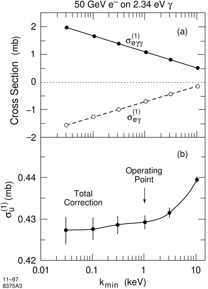
FIG. 3.: The unpolarized virtual plus soft-photon cross section $\sigma^{(1)}_{e\gamma}$ and hard-photon cross section $\sigma^{(1)}_{e\gamma\gamma}$ are shown in part (a) as functions of $k_{\gamma}^{min}$ for the case of a 50 GeV electron colliding with a 2.34 eV photon. The sum of these cross sections $\sigma_{u}^{(1)}$ is shown in part (b).

FIG. 4.: The ratio $\sigma^{(1)}_{u}/\sigma^{(0)}_{u}$ is shown in part (a) as a function of the laboratory energy of the scattered electron for the case of a 50 GeV electron colliding with a 2.34 eV photon. The difference in the fully order-$\alpha^{3}$ corrected asymmetry and the order-$\alpha^{2}$ asymmetry is shown as a function of the laboratory energy of the scattered electron in part (b). The COMRAD calculation is shown as solid lines and the calculation of Ref. [4] is shown as dashed lines.

FIG. 5.: The order-$\alpha^{2}$ cross section $\sigma^{(0)}_{u}$ and the ratio $\sigma^{(1)}_{u}/\sigma^{(0)}_{u}$ are shown in part (a) as functions of the laboratory energy of the scattered electron for the case of a 45.65 GeV electron colliding with a 2.33 eV photon. The order-$\alpha^{2}$ asymmetry function and the difference in the fully order-$\alpha^{3}$ corrected asymmetry and the order-$\alpha^{2}$ asymmetry are shown as functions of the laboratory energy of the scattered electron in part (b).

FIG. 6.: The order-$\alpha^{2}$ function $\delta\theta_{y}^{(0)}(k^{\prime}_{\rm lab})$ is plotted as the dashed curve as a function of the laboratory energy of the scattered photon for the case of a 27.5 GeV positron colliding with a 2.41 eV photon. The fractional difference in the fully order-$\alpha^{3}$ corrected function and the order-$\alpha^{2}$ function is shown the solid curve.

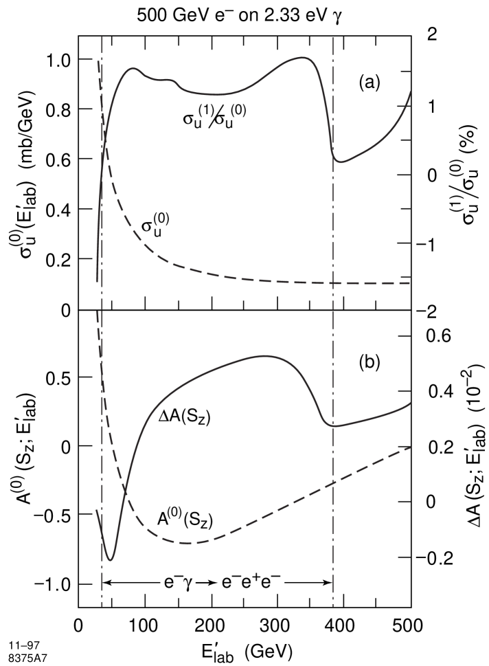
FIG. 7.: The order-$\alpha^{2}$ cross section $\sigma^{(0)}_{u}$ and the ratio $\sigma^{(1)}_{u}/\sigma^{(0)}_{u}$ are shown in part (a) as functions of the laboratory energy of the scattered electron for the case of a 500 GeV electron colliding with a 2.33 eV photon. The order-$\alpha^{2}$ asymmetry function and the difference in the fully order-$\alpha^{3}$ corrected asymmetry and the order-$\alpha^{2}$ asymmetry are shown as functions of the laboratory energy of the scattered electron in part (b). The vertical dashed-dotted lines indicate the allowed kinematic region for electrons from the $e^{-}\gamma\to e^{-}e^{+}e^{-}$ subprocess.

TABLE I.: The effect of order$-\alpha^{3}$ radiative corrections upon the analyzing powers of the SLD Compton polarimeter.

Channel	$E_{e}$ Acceptance	${\cal A}^{(0)}$	$({\cal A}-{\cal A}^{(0)})/{\cal A}^{(0)}$ (%)
7	17.14-18.02 GeV	0.7133	0.096
6	18.02-19.00 GeV	0.6483	0.097
5	19.00-20.11 GeV	0.5520	0.103
4	20.11-21.38 GeV	0.4309	0.118
3	21.38-22.83 GeV	0.2851	0.153
2	22.83-24.53 GeV	0.1228	0.285
1	24.53-26.51 GeV	$-$.0396	$-$.673

REFERENCES

- [1] L.M. Brown and R.P. Feynman, Phys. Rev. 85, 231 (1952).
- [2] W.-Y Tsai, L.L. DeRaad, and K.A. Milton, Phys. Rev. D6, 1428 (1972); K.A. Milton, W.-Y Tsai, and L.L. DeRaad, Phys. Rev. D6, 1411 (1972).
- [3] A. Góngora-T and R.G. Stuart, Z. Phys. C42, 617 (1989).
- [4] H. Veltman, Phys. Rev. D40, 2810 (1989); Erratum: Phys. Rev. D42, 1856 (1990).
- [5] K. Abe et al., Phys. Rev. Lett. 70, 2515 (1993); K. Abe et al., Phys. Rev. Lett. 73, 25 (1994); K. Abe et al., Phys. Rev. Lett. 78, 2075 (1997); R.E. Frey, OREXP-97-03, October 1997, hep-ex/9710016.
- [6] J. Timmermans, Proceedings of the 18th International Symposium on Lepton-Photon Interactions, 28 July - 1 August 1997, Hamburg, Germany.
- [7] R. Kleiss and W.J. Stirling, Nucl. Phys. B262, 235 (1985); R. Kleiss and W.J. Stirling, Phys. Lett. B179, 159 (1986); R. Kleiss, Z. Phys. C33, 433 (1987).
- [8] This expression differs by a factor of from Eq. 1 of Ref. [2] because the spinors in that work are normalized to unity.
- [9] The azimuth is defined in any frame which has been rotated such that the electron direction defines the z-axis.
- [10] W.A. Bardeen and W.-K. Tung, Phys. Rev. 173, 1423 (1968); Erratum: Phys. Rev. D4, 3229 (1971).
- [11] D.P. Barber, et al., Nucl. Inst. Meth. A338, 166 (1994); D.P. Barber, et al., Phys. Lett. B343, 436 (1995).
- [12] D.P. Barber, et al., Nucl. Inst. Meth. A329, 79 (1993).
- [13] A. Most, Proceedings of the 12th International Symposium on High-Energy Spin Physics, Amsterdam, The Netherlands (1996), p. 800.
- [14] The code COMRAD generally conforms to the Fortran-77 specification except that it performs COMPLEX*16 operations which are implemented in many compilers. The code has been successfully compiled and run with the IBM-AIX, SUN-Solaris, and DEC-OpenVMS operating systems.