$B$ and $D$ Meson Decay Constants in Lattice QCD

Abstract

We have calculated the decay constants of $B$ and $D$ mesons with lattice QCD. We use an ${\cal O}(a)$ improved action that takes light quark actions as a starting point, tuned so that it can be directly applied at the physical masses of the $b$ and $c$ quarks. Our results are $f_{B}=164\hskip-5.0pt\raisebox{0.80002pt}{\scriptsize{$\;\begin{array}[]{@{}l@{}}\makebox[15.0pt][c]{$+$}\makebox[3.5pt][r]{14\hfill}\\[-1.68004pt] \makebox[15.0pt][c]{$-$}\makebox[3.5pt][r]{11\hfill}\end{array}$}}\pm 8$ MeV, $f_{B_{s}}=185\hskip-5.0pt\raisebox{0.80002pt}{\scriptsize{$\;\begin{array}[]{@{}l@{}}\makebox[15.0pt][c]{$+$}\makebox[3.5pt][r]{13\hfill}\\[-1.68004pt] \makebox[15.0pt][c]{$-$}\makebox[3.5pt][r]{8\hfill}\end{array}$}}\pm 9$ MeV, $f_{D}=194\hskip-5.0pt\raisebox{0.80002pt}{\scriptsize{$\;\begin{array}[]{@{}l@{}}\makebox[15.0pt][c]{$+$}\makebox[3.5pt][r]{14\hfill}\\[-1.68004pt] \makebox[15.0pt][c]{$-$}\makebox[3.5pt][r]{10\hfill}\end{array}$}}\pm 10$ MeV, and $f_{D_{s}}=213\hskip-5.0pt\raisebox{0.80002pt}{\scriptsize{$\;\begin{array}[]{@{}l@{}}\makebox[15.0pt][c]{$+$}\makebox[3.5pt][r]{14\hfill}\\[-1.68004pt] \makebox[15.0pt][c]{$-$}\makebox[3.5pt][r]{11\hfill}\end{array}$}}\pm 11$ MeV in the quenched approximation. The first error in each case is statistical, and the second is from perturbation theory. We show that discretization errors are under control in our approach, and smaller than our statistical errors. The effects of the quenched approximation may raise our quenched result by up to 10%.

1 Introduction

This paper uses lattice QCD to calculate the decay constants of $B$ and $D$ mesons using an ${\cal O}(a)$ improved action that takes light quark actions as a starting point, tuned so that it can be directly applied at the physical masses of the $b$ and $c$ quarks. The $B$ meson decay constant, $f_{B}$, is of particular phenomenological interest, since it is responsible for most of the uncertainty in current determinations of the Cabibbo-Kobayashi-Maskawa matrix element $V_{td}$ from $B\overline{B}$ mixing. Recent calculations of the decay constants of $B$ mesons give much lower values than the earliest calculations done in the static approximation because of several effects, all of which happened to be negative. Perturbative corrections turn out to be large and negative. The static approximation has larger statistical errors than methods with propagating quarks. This led to contamination from excited states, which raised the estimate of $f_{B}$. The use of smeared sources and propagating quark methods mitigate this problem. The ${\cal O}(a)$ finite lattice spacing corrections likewise turned out to be large and negative.

Conversely, the earliest results for lighter quarks tended to be too low. They were done using naive light quark methods with an incorrect and singular quark field normalization which forced $f_{M}\sqrt{M}\rightarrow 0$ in the heavy quark limit.

The combination of a too high $f_{B}\sqrt{M_{B}}$ from the static approximation and a too low $f_{D}\sqrt{M_{D}}$ from light quark methods led to very large estimates of the $1/M$ corrections to $f_{M}\sqrt{M}$ in the static limit. With more recent results, including those presented here, the $1/M$ corrections are much reduced. Refs. [1] and [2] contain reviews of some of the early work.

Currently convenient inverse lattice spacings are no larger than $a^{-1}\approx$ 2 or 3 GeV. Therefore, discretization errors that go like the quark mass in lattice units, $ma$, to a power are unpleasantly large for the $c$ quark and completely out of control for the $b$ quark. This means that standard light quark formulations for lattice fermion actions cannot be used unaltered for the $b$ quark.

There are several ways of approximating heavy quarks in lattice QCD calculations with control over discretization errors. These include Nonrelativistic QCD [3, 4, 5] (NRQCD), the static approximation [6, 7], and the approach of this paper, described in Refs. [8, 9]. The methods vary significantly both in ease of application and in suitability for various calculations. The last takes the light quark actions of Wilson [10] and Sheikholeslami and Wohlert (SW) [11] as its leading approximation but adds correction operators that end up resembling those of NRQCD rather than those of the standard Symanzik improvement program. Sec. 2 contains a general discussion of the various methods for heavy quarks. It comments on our bettered understanding about which methods work best in which situations, not all of which was expected in advance. Sec. 3 treats in detail the particular form of the action used in this paper. Our numerical results are presented in Sec. 4, and compared with other recent results in Sec. 5.

2 Methods for Heavy Quarks on the Lattice

This work uses a formalism for propagating heavy quarks that reduces to the ordinary light quark formalism in the light quark limit [8, 9]. We begin by comparing the various lattice approaches to heavy quarks. NRQCD is based on an expansion in nonrelativistic operators (rotationally invariant but not Lorentz invariant) similar to that used in calculating relativistic corrections in the hydrogen atom. It can be thought of as arising from a discretization of the action arising after a Foldy-Wouthuysen-Tani (FWT) transformation of the quark fields:

$$\psi\rightarrow\exp(\theta D_{i}\gamma_{i})\psi,$$ (1)

with $\theta$ chosen so that

$$\ D\!\!\!\!/+m \rightarrow D_{0}\gamma_{0}+m$$ (2)

$$- \frac{{\bf D}^{2}}{2m}-\frac{({\bf D}^{2})^{2}}{8m^{3}}+\ldots.$$

The rest mass term does not affect the dynamics of nonrelativistic particles and is conventionally removed. Increasing accuracy is achieved by truncating the series with increasing numbers of terms.

In $B$ physics, one can use the simplest of all the methods, the static approximation, which is the truncation of the preceding series to a single term. Then the heavy quark propagator is a simple Wilson line in the time direction. It is most useful for the heaviest quarks. It is not much used recently because it has a much worse signal to noise ratio than methods using propagating quarks, which is clear in retrospect but was not foreseen.

The third method, used in this paper, can be thought of as arising from a partial FWT transformation:

$$\psi\rightarrow\exp(\theta^{\prime}D_{i}\gamma_{i})\psi,$$ (3)

and

$$D\!\!\!\!/+m \rightarrow D_{0}\gamma_{0}+m+a_{1}D_{i}\gamma_{i}$$ (4)

$$- a_{2}\left(\frac{{\bf D}^{2}}{2m}+\ldots\right),$$

where $\theta^{\prime}<\theta$. This appears to be a crazy thing to do, producing an action that combines the defects of the transformed and the untransformed actions. On the other hand, it turns out that this is the action we have been using for a long time. The Wilson and SW actions have just this form. In addition to the usual $\overline{\psi}D\!\!\!\!/\psi$ term, the $\overline{\psi}D^{2}\psi$ term added to cure the doubling problem also contributes to the kinetic energy, as in Eqn. 4. The relative strengths of the two terms change as $ma$ is increased.

For the Wilson action, $a_{1}=1$, and $a_{2}=ma$. These have the property that the nonrelativistic $\overline{\psi}D^{2}\psi$ term takes over automatically from the Dirac-style kinetic energy term $\overline{\psi}D\!\!\!\!/\psi$ as $ma\rightarrow\infty$ in the Wilson action. The Wilson action turns into a nonrelativistic action in the large mass limit. The heavy quarks in heavy-light mesons are highly nonrelativistic. ($p/m_{ch}\sim\Lambda_{\rm QCD}/m_{ch}\sim.2$ and $p/m_{b}\sim.06$.) Therefore, it is the Wilson term, rather than the Dirac term, that contributes most to the heavy quark kinetic energy.

We can write a lattice energy-momentum relation

$$E^{2}=M_{1}^{2}+\frac{M_{1}}{M_{2}}{p}^{2}+\ldots,$$ (5)

where the “rest mass”

$$M_{1}=E({0}),$$ (6)

and the “kinetic mass”

$$M_{2}^{-1}=(\partial^{2}E/\partial p_{i}^{2})_{{\scriptstyle p}={0}}.$$ (7)

The Wilson action and most other actions have the property that $M_{1}$ does not equal $M_{2}$ for $ma\neq 0$. For nonrelativistic particles, the rest mass does not affect the dynamics and the kinetic mass governs the leading important term. Therefore, the rest mass is normally simply omitted from the action in NRQCD and in the static approximation, although there is no harm (and no benefit) in including it. However, it cannot be set to zero if one wishes to recover a sensible light quark limit. It is easy to find a Wilson style action which does satisfy $M_{1}=M_{2}$ by letting the hopping parameter for the time direction, $\kappa_{t}$, differ from the one in the spatial directions, $\kappa_{s}$. The two $\kappa$’s can be separately tuned so that $M_{1}=M_{2}$ with no loss of predictive power, by requiring Lorentz invariance in Eqn. 5. Nevertheless, since $M_{1}$ doesn’t affect the physics of nonrelativistic systems, the Wilson and SW actions can be used without problems for nonrelativistic systems as long as the kinetic mass, and not the rest mass, is used to set the quark mass. We can use $\kappa_{t}=\kappa_{s}$ with an incorrect $M_{1}$ and a correct $M_{2}$.

The Wilson and SW actions and the action of NRQCD all use one-hop time derivatives. When the action includes a large rest mass, this is a requirement, since two-hop time derivatives introduce new states with complex energies when $ma>1$. Therefore, heavy-quark improvements of the Wilson action cannot follow the conventional Symanzik program of adding two-hop space-like and time-like interactions at ${\cal O}(a^{2})$, but must follow NRQCD and correct only the spatial interactions. The existence of the transfer matrix and the Hamiltonian ensures that this is possible.

The parameters of the action in our approach must have nontrivial mass dependence, just as those of NRQCD do. For $ma>1$, the wave function normalization, the relation between the physical mass and the hopping parameter, etc., are completely different from their $ma=0$ values. When $ma<1$, this mass dependence may be expanded in power series. For the Wilson and SW Lagrangians, this yields just the usual series of operators, with the same coefficients. If the mass dependent coefficients in our style of interpreting the Lagrangian,

$${\cal L} = m(am)\overline{\psi}\psi+z(am)\overline{\psi}D\!\!\!\!/\psi+c(am)\overline{\psi}\sigma_{\mu\nu}F_{\mu\nu}\psi+\ldots,$$ (8)

are expanded, the usual series of powers of $ma$ multiplying identical operators must result:

$${\cal L} = m\overline{\psi}\psi+a_{1}m^{2}a\overline{\psi}\psi+\ldots$$ (9)

$$+ z\overline{\psi}D\!\!\!\!/\psi+z_{1}ma\overline{\psi}D\!\!\!\!/\psi+z_{2}m^{2}a^{2}\overline{\psi}D\!\!\!\!/\psi+\ldots$$

$$+ c_{SW}\overline{\psi}\sigma_{\mu\nu}F_{\mu\nu}\psi+c_{2}ma\overline{\psi}\sigma_{\mu\nu}F_{\mu\nu}\psi+\ldots.$$

Sometimes in the Symanzik program, $\overline{\psi}\sigma_{\mu\nu}F_{\mu\nu}\psi$ and $ma\overline{\psi}\sigma_{\mu\nu}F_{\mu\nu}\psi$ are spoken of as if they were totally unrelated operators. Even for light quarks, it makes more sense to think of them as different terms in an $ma$ expansion of an $ma$ dependent coefficient analogous to the expansion in $\alpha_{s}$ of an $\alpha_{s}$ dependent coefficient. The fact that coefficients in the usual approach blow up as $ma\rightarrow\infty$ is a property of the expansion and not of the required functions in Eqn. 8 themselves. They stay well behaved if sensible normalization conditions are applied.

With the added ingredient of decoupling the timelike and spacelike parts of operators, it becomes possible to formulate an action that is systematically improvable, even for large $ma$. While for $ma>1$ the action becomes very similar to NRQCD in its behavior, for $ma<1$ it may be regarded as a resummation of the usual operators of the Wilson and SW actions to all orders in $m$.

For physics involving the $b$ quark, NRQCD methods are often easier and therefore more accurate. Taking the $ma\ll 1$ limit is not possible, but correction operators are not too hard to organize and add. This is particularly important in the $\Upsilon$ system, where momenta are rather large, and correction operators are important in obtaining such things as the correct spin-dependent spectrum. In $B$ mesons, on the other hand, the $b$ quarks are extremely nonrelativistic. $(v/c)^{2}\sim(0.3\ {\rm GeV}/5.0\ {\rm GeV})^{2}\sim 0.3\%$. Therefore, only the first few operators in the action, which are the same in the two methods, are important. As long as these are normalized in the same way, it matters little what additional operators are hanging around. Therefore, in $B$ mesons the effects of the differences between NRQCD and our heavy quark methods are minimal, and the two methods should yield nearly identical results.

For physics involving the $c$ quark, heavy quark methods that can recover a relativistic form of the action are often easier and more accurate. The series in $v^{2}$ is less convergent, so eliminating the need for it by taking $a$ toward zero while recovering a relativistic action may be more convenient. For hadrons containing charmed quarks, it is possible to do calculations with the Wilson and SW actions even with the old interpretation of the coefficients. However, since $m_{ch}a\approx 5a\Lambda_{QCD}$, our ability to sum up the required series in $ma$ exactly is likely to produce a faster approach to the continuum limit than naive light quark methods.

For physics involving either the $b$ or $c$ quarks, both NRQCD and our method can be used successfully. Even when one works better or worse than the other, we still learn something.

3 The Action Used in this Calculation

We have used the approach for heavy quarks outlined above to calculate the decay constants of the $D$, $D_{s}$, $B$, and $B_{s}$ mesons. We start with an action corrected to ${\cal O}(a)$, which in general is

$$S = {\displaystyle\sum_{n}}\bar{\psi}_{n}\psi_{n}$$ (10)

$$- \kappa_{t}{\displaystyle\sum_{n}}\left[\rule{0.0pt}{9.70001pt}\bar{\psi}_{n}(1-\gamma_{0})U_{n,0}\psi_{n+\hat{0}}+\bar{\psi}_{n+\hat{0}}(1+\gamma_{0})U^{\dagger}_{n,0}\psi_{n}\right]$$

$$- \,\kappa_{s}{\displaystyle\sum_{n,i}}\left[\rule{0.0pt}{9.70001pt}\bar{\psi}_{n}(1-\gamma_{i})U_{n,i}\psi_{n+\hat{\imath}}+\bar{\psi}_{n+\hat{\imath}}(1+\gamma_{i})U_{n,i}^{\dagger}\psi_{n}\right]$$

$$+ \mbox{\small$\frac{i}{2}$}c_{B}\kappa_{s}\sum_{n;i,j,k}\varepsilon_{ijk}\bar{\psi}_{n}\sigma_{ij}B_{n;k}\psi_{n}$$

$$+ ic_{E}\kappa_{s}\sum_{n;i}\bar{\psi}_{n}\sigma_{0i}E_{n;i}\psi_{n}.$$

The second and third terms are the timelike and spacelike pieces of the kinetic energy of the Wilson action. The fourth and fifth terms are the spacelike and timelike pieces of the SW correction operator.

The action used to calculate $f_{M}\sqrt{M}$ may be simplified from this form. As previously noted, when $ma\neq 0$, we find that $M_{1}\neq M_{2}$ and that higher orders in $p$ in Eqn. 5 do not vanish as they should. Explicitly, we define

$$ma=\frac{1}{2\kappa_{t}}-[1+3\zeta],$$ (11)

where $\zeta\equiv\kappa_{s}/\kappa_{t}$. Then we can calculate the free lattice propagator and expand in $pa$ to derive

$$M_{1}a=\log(1+ma),$$ (12)

and

$$\frac{1}{M_{2}a}=\frac{2\zeta^{2}}{ma(2+ma)}+\frac{\zeta}{1+ma}.$$ (13)

For nonrelativistic fermions, the physics of the system is influenced hardly at all by the rest mass $M_{1}$. $M_{2}$ controls the leading order dynamics. We can therefore set

$$\kappa_{t}=\kappa_{s}=\kappa,$$ (14)

but we must tune $\kappa$ so that $M_{2}$ equals the physical quark mass.

Likewise, the physics of heavy-light mesons is insensitive to the final, spin-orbit term in Eqn. 10. (This not true of some other quantities in heavy quark physics, such as the fine structure of quarkonia.) We can therefore set

$$c_{E}=c_{B}=c,$$ (15)

and tune $c$ to get the physics of the fourth operator in Eqn. 10, the $\bf\sigma\cdot B$ operator, correct. At tree level, this requires the same value that it has for light quarks in the SW action, $c=c_{SW}=1$.

The decay constant $f_{M}$ parametrizes the matrix element

$$\langle 0|A_{\mu}|M,{p}\rangle=p_{\mu}f_{M}$$ (16)

of the axial vector current between the pseudoscalar meson $M$ and the vacuum. Here the state $|M,{p}\rangle$ has the standard, relativistic normalization. Like the action, the axial vector current $A_{\mu}$ must be specified through ${\cal O}(a)$. At tree level we take

$$A_{\mu}=2\sqrt{\kappa_{t,h}\kappa_{t,l}}Z_{A}\bar{\Psi}_{h}\gamma_{\mu}\gamma_{5}\Psi_{l},$$ (17)

where the subscripts $h$ and $l$ denote the heavy and light quarks, $Z_{A}$ is a mass-dependent (re)normalization factor, and $\Psi$ denotes a (rotated) field, specified below.

The factors $\sqrt{2\kappa}$ arise from naive quark wave function mass dependence in long historical use. Wilson used the field normalization

$$z_{\rm wf}^{\rm naive}=\sqrt{2\kappa}$$ (18)

for massless fermions [10]. It is easy to see that this is correct only in the $ma=0$ limit that Wilson was considering. Away from $ma=0$, a straightforward examination of the free propagator shows that, if the quarks are to have their conventional canonical normalizations, the correct normalization is

$$z_{\rm wf}=\sqrt{1-6\kappa}$$ (19)

for the Wilson and SW actions, or

$$z_{\rm wf}=\sqrt{1-6\kappa_{s}}$$ (20)

if $\kappa_{t}\neq\kappa_{s}$. These are equal to the conventional but incorrect normalization for $ma=0$: $\sqrt{2\kappa}=\sqrt{1-6\kappa}=1/2$. As $m_{h}a\to\infty$ ($\kappa_{t,h}\to 0$), the naive normalizations force $f_{M}$ incorrectly to zero, unless the mass dependence of $Z_{A}$ compensates accordingly. Indeed, the early estimates of $f_{D}$ that were too low stem from the naive assumption $Z_{A}\approx 1$, even when $m_{h}a\sim 1$. Combining Eqns. 18 and 20, we see that

$$Z_{A} = \sqrt{\frac{1-6\kappa_{s,h}}{2\kappa_{t,h}}\frac{1-6\kappa_{s,l}}{2\kappa_{t,l}}}$$ (21)

$$= \sqrt{(1+m_{h}a)(1+m_{l}a)},$$ (22)

where the second expression follows from Eqn. 11.

The remaining ingredient of Eqn. 17 is the rotated field

$$\Psi=(1+d_{1}\ {\gamma_{i}}{D_{i}})\psi,$$ (23)

where $i$ is summed over the three spatial directions and, at tree level,

$$d_{1}=\frac{\zeta(1+ma)}{ma(2+ma)}-\frac{1}{2M_{2}a}.$$ (24)

The second term of $d_{1}$ is the same as the $1/m$ correction present in NRQCD. It is a consequence of the Foldy-Wouthuysen-Tani transformation in Eqn. 1. The first term of $d_{1}$ allows for the fact that the implicit Foldy-Wouthuysen-Tani transformation of Wilson-like actions takes $\theta^{\prime}\neq\theta$. The numerical value of $d_{1}$ depends on the tuning of $\zeta=\kappa_{s}/\kappa_{t}$. In most cases, and in particular when $\zeta=1$, the contribution to $f_{M}$ proportional to $d_{1}$ is ${\cal O}(m\Lambda a^{2})$ when $ma\ll 1$, but ${\cal O}(\Lambda/m)$ when $ma\gg 1$. In the latter region it is essential to include it, if one is interested in the $1/m_{h}$ corrections to the static limit. It also makes sense to include the rotation when $ma<1$.

The dominant mass-dependence exhibited in Eqn. 21 persists beyond tree level [8]. Quantum effects require further terms to be added to the right-hand side of Eqn. 17 to construct an ${\cal O}(a)$-improved axial vector current. In our numerical work we neglect them and we set $d_{1}$ to its tree-level, mean-field improved value.

Thus, to ${\cal O}(a^{0})$ and ${\cal O}(a^{1})$, we can use precisely the Wilson and the SW actions for much heavy quark physics. In this paper we will use the SW action:

$$S = {\displaystyle\sum_{n}}\bar{\psi}_{n}\psi_{n}$$ (25)

$$- \,\kappa{\displaystyle\sum_{n,\mu}}\left[\rule{0.0pt}{9.70001pt}\bar{\psi}_{n}(1-\gamma_{\mu})U_{n,\mu}\psi_{n+\hat{\imath}}+\bar{\psi}_{n+\hat{\imath}}(1+\gamma_{\mu})U_{n,\mu}^{\dagger}\psi_{n}\right]$$

$$+ \mbox{\small$\frac{i}{2}$}c_{SW}\kappa\sum_{n;\mu\nu}\bar{\psi}_{n}\sigma_{\mu\nu}F_{n;\mu\nu}\psi_{n}.$$

There are two key differences between our use of this action for heavy quarks and the naive approach.

1. The use of the correctly normalized quark fields and currents, and the additional three dimensional field rotation for the heavy quark in the currents.

2. The use of the kinetic mass rather than the rest mass to set the quark mass.

At higher orders in $a$, it is no longer true that ordinary forms of the light quark action may be used for heavy quarks. Two-hop corrections for time derivatives cannot be used since they introduce new states with energies which become complex when $ma>1$. ${\cal O}(a^{2})$ corrections must have a nonrelativistic form as in NRQCD.

Having determined the coefficients in the action at tree level, we now discuss their renormalization. In general, the coefficients $c_{n}$ of operators $O_{n}$ in a Wilsonian effective action depend on the physical parameters of the theory and on the renormalization scale. For lattice QCD we can write

$$S(m/\Lambda_{QCD},\Lambda_{QCD}\ a)=\sum_{n}c_{n}(ma,\alpha_{s})O_{n},$$ (26)

where $m$ and $\alpha_{s}$ are the bare parameters of the lattice theory. In the usual Symanzik approach, these coefficients are expanded both in $\alpha_{s}$ and in $ma$. It is usually an advantage if an expansion in $\alpha_{s}$ can be avoided. Likewise, as remarked earlier, there is an advantage in not expanding in $ma$. The expansion in $ma$ is the source of the breakdown of the method for $ma>1$. If the $c_{n}$ are not expanded in $ma$, applying standard normalization conditions yields well behaved $c_{n}$ for large $ma$, as shown at tree level for a few important cases above. It is of course necessary that this is true for the $c_{n}$ in the full quantum theory as well.

Most quantum corrections done so far have only been calculated in perturbation theory. It is clear that the tadpoles, which dominate many lattice perturbation theory calculations, create well-behaved contributions to the renormalization of these actions at all quark masses. Tadpole-improved perturbation theory [12] suggests that the dominant perturbative correction to the renormalization of coefficients of operators is given by short distance tadpoles. They can be estimated by noting that the link $U_{\mu}=1+ig_{0}A_{\mu}-\frac{1}{2}g_{0}^{2}A_{\mu}^{2}+\ldots$ does not fluctuate around 1, as is implicitly assumed in the usual perturbative expansion, but around some smaller value, $u_{0}$. The so-called mean link $u_{0}$ can be estimated from the expectation value of any link-containing operator such as the plaquette ($\langle U_{P}\rangle=u_{0}^{4}$) or the expectation value of $U_{\mu}$ itself in Landau gauge. By counting links in the actions Eqn. 10 or Eqn. 25 one can see that the usual tadpole estimates of corrections to operator coefficients $\tilde{\kappa}=\kappa u_{0}$ and $\tilde{c}_{SW}=c_{SW}u_{0}^{3}$ are still valid for heavy quarks even though the one-loop coefficients differ slightly.

The one-loop coefficients which have been calculated so far have the required property that they stay small and well-behaved as $ma$ is varied from 0 to $\infty$ [13, 14]. The part of the one-loop correction to the local heavy-light axial vector current arising from the leading operators in the SW action has been calculated by Aoki et al. [15]. It also is well-behaved for all quark masses, and has been incorporated into our results. The part of the correction arising from the ${\cal O}(a)$ correction to the axial vector current is currently being calculated [16].

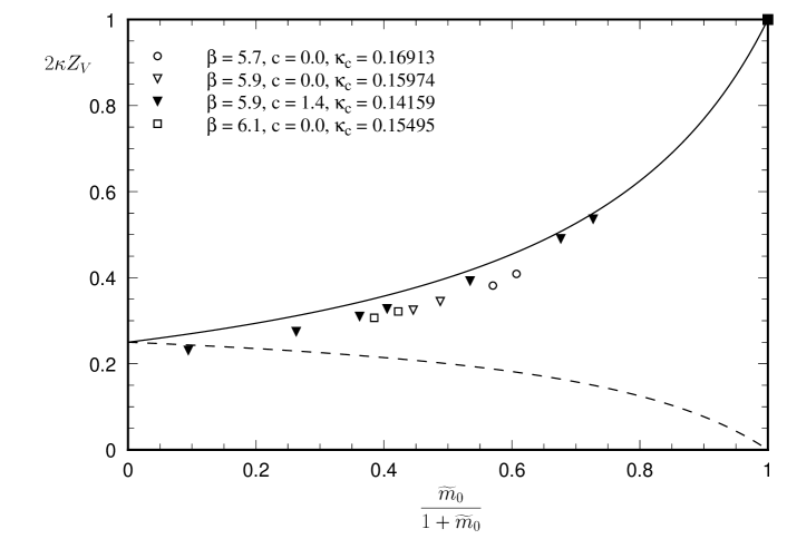
Figure 1: The current normalization factor $2\kappa Z_{V}$ calculated nonperturbatively from the quantity $\langle J/\psi|V_{4}|J/\psi\rangle$, where the (unnormalized) local charge $V_{4}=\overline{\psi}\gamma_{0}\psi$ should simply count the numbers of fermions when properly normalized. The upper curve is $1-6\tilde{\kappa}$, from mean-field improving Eqn. 19. The lower curve is the naive ansatz $2\tilde{\kappa}$.

One important quantity can be easily computed nonperturbatively, to see that the required good behavior persists to all orders of perturbation theory. This is the quark wave function renormalization, which is required for all current renormalizations. This is part of the vector current, which is easy to normalize nonperturbatively by inserting the charge into any physical state, such as a 1S quarkonium state [8]. Fig. 1 shows the result of such a calculation, compared with the tadpole improved tree-level correct normalization and the naive normalization. The vector current normalization factor $Z_{V}$ is defined analogously to the axial vector normalization factor $Z_{A}$ in Eqn. 21. It is easy to see that the good behavior of the correct normalization in Eqn. 19 is preserved when full quantum effects are included nonperturbatively.

4 Numerical Results

$\beta$	6.1	5.9	5.7
Volume	$24\times 48$	$16\times 32$	$12\times 24$
Configurations	100	350	300
$c_{\rm SW}$	1.46	1.50	1.57
$\alpha_{V}(1/a)$	0.222	0.259	0.330
$\alpha_{V}(2/a)$	0.171	0.192	0.227
$\alpha_{V}(\pi/a)$	0.149	0.164	0.189
$u_{0}$	0.8816	0.8734	0.8608
$\kappa_{l}$	0.1372	0.1382	0.1405
	0.1373	0.1385	0.1410
	0.1376	0.1388	0.1415
	0.1379	0.1391	0.1419
		0.1394
$\kappa_{h}$	0.050	0.050	0.050
	0.099	0.093	0.070
	0.126	0.1227	0.089
		0.126	0.110
			0.119
$a^{-1}(f_{K})$ (GeV)	2.21$\;\begin{array}[]{@{}l@{}}\makebox[15.0pt][c]{$+$}\makebox[1.75pt][r]{7\hfill}\\[-0.83997pt] \makebox[15.0pt][c]{$-$}\makebox[1.75pt][r]{3\hfill}\end{array}$	1.57$\;\begin{array}[]{@{}l@{}}\makebox[15.0pt][c]{$+$}\makebox[1.75pt][r]{3\hfill}\\[-0.83997pt] \makebox[15.0pt][c]{$-$}\makebox[1.75pt][r]{2\hfill}\end{array}$	1.01$\;\begin{array}[]{@{}l@{}}\makebox[15.0pt][c]{$+$}\makebox[1.75pt][r]{2\hfill}\\[-0.83997pt] \makebox[15.0pt][c]{$-$}\makebox[1.75pt][r]{1\hfill}\end{array}$
$a^{-1}(1P-1S)$ (GeV)	2.62$\;\begin{array}[]{@{}l@{}}\makebox[15.0pt][c]{$+$}\makebox[1.75pt][r]{8\hfill}\\[-0.83997pt] \makebox[15.0pt][c]{$-$}\makebox[1.75pt][r]{9\hfill}\end{array}$	1.80$\;\begin{array}[]{@{}l@{}}\makebox[15.0pt][c]{$+$}\makebox[1.75pt][r]{5\hfill}\\[-0.83997pt] \makebox[15.0pt][c]{$-$}\makebox[1.75pt][r]{5\hfill}\end{array}$	1.16$\;\begin{array}[]{@{}l@{}}\makebox[15.0pt][c]{$+$}\makebox[1.75pt][r]{3\hfill}\\[-0.83997pt] \makebox[15.0pt][c]{$-$}\makebox[1.75pt][r]{3\hfill}\end{array}$

Table 1: Parameters used in the numerical calculations.

We turn now to a discussion of our numerical results. A preliminary version of our results appeared in Ref. [18]. In Table 1 we show some details of our calculations. The light quark propagators are the same ones used to determine the light quark masses in Ref [17]. They were calculated with the SW action using a mean-field improved coefficient $c_{SW}$. $\alpha_{V}(1/a)$, $\alpha_{V}(2/a)$, and $\alpha_{V}(\pi/a)$, defined as in Ref. [12], are values of the strong coupling constant at several relevant scales. $u_{0}$ is the mean link used in tadpole improvement. $\kappa_{l}$ and $\kappa_{h}$ are the hopping parameters used for the light and heavy quarks, respectively. $a^{-1}(f_{K})$ and $a^{-1}$(1P-1S) are the lattice spacings in physical units as determined by $f_{K}$ and the 1P–1S splitting of charmonium, respectively. For $\beta=$ 6.1, 5.9, and 5.7, the hopping parameters closest to the $b$ hopping parameters are $\kappa_{b}\approx$ 0.099, 0.093, and 0.089 respectively. Those closest to charm are $\kappa_{ch}\approx$ 0.126, 0.1227, and 0.119 respectively. The hopping parameters closest to strange are 0.1373, 0.1385, and 0.1405 respectively. Only modest interpolations in quark mass are necessary for $B_{s}$ and $D_{s}$ mesons. $B$ and $D$ physics must be obtained by chiral extrapolation to the physical light mass limit. Charm and bottom $\kappa$’s were obtained by demanding that spin-averaged kinetic masses of the 1S charmonium and bottomium states match experiment. For the strange quark, the hopping parameter was fixed from the kaon mass. We have also done calculations with static propagators for the heavy quarks, which corresponds in our notation to $\kappa_{s}=0$ and $\kappa_{t}=1/2$.

Figure 2: Chiral extrapolations of $f_{B}\sqrt{M_{B}}$ to $m=0$ at $\beta=5.7$ (top), $\beta=5.9$ (center), and $\beta=6.1$ (bottom).

Masses and matrix elements were obtained from minimizing $\chi^{2}$’s using the the full correlation matrix. Decay constants were obtained by dividing matrix elements by the square root of the experimentally measured meson mass. Statistical errors were calculated with the bootstrap method, using 1000 bootstrap samples in each fit. Chiral extrapolations of $f_{B}\sqrt{M_{B}}$ at $\beta=$ 6.1, 5.9, and 5.7 are shown in Fig. 2. No problems with $\chi^{2}$ using linear fits were observed with the $\kappa_{l}$’s shown. In runs at lower quark masses, which we did not use here, occasional exceptional configurations and poor $\chi^{2}$’s began to appear.

The possibility of contamination of the results by excited states was checked by testing for consistency of one-, two-, and three-state fits using $\delta$ function, 1S, and 2S sources at both source and sink. In the sources, one quark is smeared with the supposed wave function and the other is a delta function. Shapes of the 1S and 2S sources were taken from lattice Coulomb gauge valence quark wave functions of the $B$ and $D$ mesons. Fig. 3 shows a comparison of one- and two-state fits. The measured energy splitting between the ground and first excited states and the observed agreement between the ground state energies obtained in one- and two-state fits suggests that the contamination from excited states is small in the region used for fitting. The measured values of $f_{M}\sqrt{M}$ in one-state fits and two-state fits agreed to within statistical errors.

Figure 3: Comparison of results of one- and two-state fits at $\beta=5.9$, $\kappa_{h}=0.1227$ (near $\kappa_{ch}$), and $\kappa_{l}=0.1385$ (near $\kappa_{s}$). Good consistency between the two is observed in the fit range for the lightest state.

The dominant finite lattice spacing errors for the Wilson action are ${\cal O}(a)$. When these have been removed, as they have been in the SW action, the remaining finite $a$ dependence arises from a combination of ${\cal O}(\alpha_{s}^{2})$, ${\cal O}(\alpha_{s}a)$, and ${\cal O}(a^{2})$. This means that attempts to extrapolate away any remaining finite $a$ dependence are uncertain, since we do not have a theory of the functional form of the remaining dependence. The ideal situation when using improved actions is negligible dependence of the results on $a$. As shown in Figs. 4 and 5, to within statistical errors, this has been achieved if $f_{K}$ is used to determine the lattice spacing. The results extrapolated to zero lattice spacing are consistent with the results at the smallest lattice spacings. Thus, within our statistical errors we do not find any evidence for discretization errors.

The least understood source of uncertainty is due to the quenched approximation (the omission of sea quarks). One effect of the quenched approximation is that different answers for decay constants will be obtained depending on which physical quantity is used to set the lattice spacing in physical units. The appendix tabulates results using $f_{K}$, $f_{\pi}$ and the 1P–1S splitting in charmonium to set the scale. The well-measured physical quantity which most resembles the heavy-light decay constants is $f_{K}$. It therefore offers the best chance that some statistical, systematic, and especially quenching errors in $f_{M}$ will cancel out. It is relatively easy to determine numerically. ($f_{\pi}$, for example, requires an additional chiral extrapolation which introduces larger statistical error and unreliability. Our $K$ consists of two degenerate quarks of mass $(m_{s}+m_{d})/2$.) Taking $a^{-1}$ from $f_{K}$ has the pragmatic defect that it yields $f_{M}$’s that lie at the bottom of the range given by all of the standard methods of setting the lattice spacing, so that removing the quenched approximation is more likely to move the results up than down. One way of estimating the effect of the quenched approximation is to examine the spread of values obtained by setting the lattice spacing in various reasonable ways. However, as shown in the appendix, quantities similar to $f_{M}$ tend to give similar results, while quantities more dissimilar, such as quarkonia spectra, can give results quite a bit different. It is not easy to quantify what is “reasonable”. The most quantitative estimate so far of estimating the effects of quenching with actual unquenched calculations was given in Ref. [19]. It compares results for quenched and unquenched calculations done in similar ways. They report quenching uncertainties of around ${}_{-0}^{+5}\%$ for the $D$ and $D_{s}$ mesons, and ${}_{-0}^{+10}\%$ for the $B$ and $B_{s}$.

Figure 4: $f_{B}\sqrt{M_{B}}$ and $f_{D}\sqrt{M_{D}}$ extrapolated to zero lattice spacing. The statistical error bands are 1 $\sigma$ ranges of linear extrapolations found in bootstrap runs.

Figure 5: $f_{B_{s}}\sqrt{M_{B_{s}}}$ and $f_{D_{s}}\sqrt{M_{D_{s}}}$ extrapolated to zero lattice spacing.

We now summarize our results and uncertainties. In Figs. 4 and 5 we show results for $f_{D}\sqrt{M_{D}}$, $f_{D_{s}}\sqrt{M_{D_{s}}}$, $f_{B}\sqrt{M_{B}}$, and $f_{B_{s}}\sqrt{M_{B_{s}}}$, using $f_{K}$ to set the lattice spacing in GeV. Our final results for the decay constants and their ratios are shown in Table 2. Statistical errors in the decay constants are obtained from bootstraps over extrapolations to $a=0$ linearly in $a$. The $\chi^{2}$’s refer to these extrapolations. Statistical errors in the ratios are obtained from bootstraps over the ratios of extrapolations thus obtained.

	Final Value	$\chi^{2}/d.o.f$
$f_{B}$	$164\hskip-5.0pt\raisebox{0.80002pt}{\scriptsize{$\;\begin{array}[]{@{}l@{}}\makebox[15.0pt][c]{$+$}\makebox[3.5pt][r]{14\hfill}\\[-1.68004pt] \makebox[15.0pt][c]{$-$}\makebox[3.5pt][r]{11\hfill}\end{array}$}}\pm 8$ MeV	1.32/1
$f_{B_{s}}$	$185\hskip-5.0pt\raisebox{0.80002pt}{\scriptsize{$\;\begin{array}[]{@{}l@{}}\makebox[15.0pt][c]{$+$}\makebox[3.5pt][r]{13\hfill}\\[-1.68004pt] \makebox[15.0pt][c]{$-$}\makebox[3.5pt][r]{8\hfill}\end{array}$}}\pm 9$ MeV	2.06/1
$f_{D}$	$194\hskip-5.0pt\raisebox{0.80002pt}{\scriptsize{$\;\begin{array}[]{@{}l@{}}\makebox[15.0pt][c]{$+$}\makebox[3.5pt][r]{14\hfill}\\[-1.68004pt] \makebox[15.0pt][c]{$-$}\makebox[3.5pt][r]{10\hfill}\end{array}$}}\pm 10$ MeV	0.77/1
$f_{D_{s}}$	$213\hskip-5.0pt\raisebox{0.80002pt}{\scriptsize{$\;\begin{array}[]{@{}l@{}}\makebox[15.0pt][c]{$+$}\makebox[3.5pt][r]{14\hfill}\\[-1.68004pt] \makebox[15.0pt][c]{$-$}\makebox[3.5pt][r]{11\hfill}\end{array}$}}\pm 11$ MeV	1.01/1
$f_{D}/f_{B}$	1.19$\;\begin{array}[]{@{}l@{}}\makebox[15.0pt][c]{$+$}\makebox[3.5pt][r]{6\hfill}\\[-1.68004pt] \makebox[15.0pt][c]{$-$}\makebox[3.5pt][r]{6\hfill}\end{array}$
$f_{D_{s}}/f_{B_{s}}$	1.14$\;\begin{array}[]{@{}l@{}}\makebox[15.0pt][c]{$+$}\makebox[3.5pt][r]{4\hfill}\\[-1.68004pt] \makebox[15.0pt][c]{$-$}\makebox[3.5pt][r]{3\hfill}\end{array}$
$f_{B_{s}}/f_{B}$	1.13$\;\begin{array}[]{@{}l@{}}\makebox[15.0pt][c]{$+$}\makebox[1.75pt][r]{5\hfill}\\[-0.83997pt] \makebox[15.0pt][c]{$-$}\makebox[1.75pt][r]{4\hfill}\end{array}$
$f_{D_{s}}/f_{D}$	1.10$\;\begin{array}[]{@{}l@{}}\makebox[15.0pt][c]{$+$}\makebox[3.5pt][r]{4\hfill}\\[-1.68004pt] \makebox[15.0pt][c]{$-$}\makebox[3.5pt][r]{3\hfill}\end{array}$
$(f_{B_{s}}/f_{B})/(f_{D_{s}}/f_{D})$	1.03$\;\begin{array}[]{@{}l@{}}\makebox[15.0pt][c]{$+$}\makebox[3.5pt][r]{4\hfill}\\[-1.68004pt] \makebox[15.0pt][c]{$-$}\makebox[3.5pt][r]{4\hfill}\end{array}$

Table 2: Final results for the decay constants and ratios in the quenched approximation. The first error for the decay constants is from statistics, the second is systematics, mostly from perturbation theory. An additional uncertainty of perhaps 10% is present in the decay constants due to the quenched approximation, as discussed in the text. The error in decay constant ratios is statistical.

A common way of estimating the uncertainties from perturbation theory is to do the perturbation theory at a range of plausible scales, say $1/a$ to $\pi/a$. That method does not give a sensible result in this case. The scale variation has a much larger effect at large $a$ than at small $a$. When the results are extrapolated linearly to $a=0$, they give the same answers to within a per cent, even though the perturbative effect being extrapolated is not at all linear in $a$. This is clearly an underestimate of the perturbative uncertainties. These are due to ${\cal O}(\alpha_{s}^{2})$ terms of order 3% plus the remaining ${\cal O}(\alpha_{s})$ term which is currently being calculated. Assuming that this term has roughly the same value that it has in NRQCD, we have taken 5% for the perturbative uncertainty.

The remaining uncertainties in the quenched approximation are likely to be smaller than the statistical and perturbative uncertainties. We do not see evidence in Figs. 4 and 5 for finite lattice spacing effects within our statistical errors. We estimate that the effects of uncertainties in the determination of the heavy quark mass are about a per cent or two. Finite volume errors are likewise expected to be small for $B$ and $D$ mesons on our lattice volumes.

Quenching uncertainty estimates of around 10% are common, based on ranges of results using different quantities to set the lattice spacing. The crude, but quantitative estimates of quenching effects in Ref. [19] are within the range of the less quantitative estimates. If we assume that the effects of the quenched approximation are similar for different quark actions, and apply the largest of their quenching uncertainties to our quenched results, we obtain, $f_{B}=164\hskip-5.0pt\raisebox{0.80002pt}{\scriptsize{$\;\begin{array}[]{@{}l@{}}\makebox[15.0pt][c]{$+$}\makebox[3.5pt][r]{14\hfill}\\[-1.68004pt] \makebox[15.0pt][c]{$-$}\makebox[3.5pt][r]{11\hfill}\end{array}$}}\pm 8\hskip-5.0pt\raisebox{0.80002pt}{\scriptsize{$\;\begin{array}[]{@{}l@{}}\makebox[15.0pt][c]{$+$}\makebox[3.5pt][r]{16\hfill}\\[-1.68004pt] \makebox[15.0pt][c]{$-$}\makebox[3.5pt][r]{0\hfill}\end{array}$}}$ MeV, $f_{B_{s}}=185\hskip-5.0pt\raisebox{0.80002pt}{\scriptsize{$\;\begin{array}[]{@{}l@{}}\makebox[15.0pt][c]{$+$}\makebox[3.5pt][r]{13\hfill}\\[-1.68004pt] \makebox[15.0pt][c]{$-$}\makebox[3.5pt][r]{8\hfill}\end{array}$}}\pm 9\hskip-5.0pt\raisebox{0.80002pt}{\scriptsize{$\;\begin{array}[]{@{}l@{}}\makebox[15.0pt][c]{$+$}\makebox[3.5pt][r]{18\hfill}\\[-1.68004pt] \makebox[15.0pt][c]{$-$}\makebox[3.5pt][r]{0\hfill}\end{array}$}}$ MeV, $f_{D}=194\hskip-5.0pt\raisebox{0.80002pt}{\scriptsize{$\;\begin{array}[]{@{}l@{}}\makebox[15.0pt][c]{$+$}\makebox[3.5pt][r]{14\hfill}\\[-1.68004pt] \makebox[15.0pt][c]{$-$}\makebox[3.5pt][r]{10\hfill}\end{array}$}}\pm 10\hskip-5.0pt\raisebox{0.80002pt}{\scriptsize{$\;\begin{array}[]{@{}l@{}}\makebox[15.0pt][c]{$+$}\makebox[3.5pt][r]{20\hfill}\\[-1.68004pt] \makebox[15.0pt][c]{$-$}\makebox[3.5pt][r]{0\hfill}\end{array}$}}$ MeV, and $f_{D_{s}}=213\hskip-5.0pt\raisebox{0.80002pt}{\scriptsize{$\;\begin{array}[]{@{}l@{}}\makebox[15.0pt][c]{$+$}\makebox[3.5pt][r]{14\hfill}\\[-1.68004pt] \makebox[15.0pt][c]{$-$}\makebox[3.5pt][r]{11\hfill}\end{array}$}}\pm 11\hskip-5.0pt\raisebox{0.80002pt}{\scriptsize{$\;\begin{array}[]{@{}l@{}}\makebox[15.0pt][c]{$+$}\makebox[3.5pt][r]{21\hfill}\\[-1.68004pt] \makebox[15.0pt][c]{$-$}\makebox[3.5pt][r]{0\hfill}\end{array}$}}$ MeV, where the uncertainties are statistical, systematic other than quenching, and quenching. The last uncertainty is less quantitative than the first two.

Perturbative errors cancel in ratios of decay constants. It is possible, but not proven, that deviations of ratios from one have quenching uncertainties of the usual 10-20% size. In that case they would be significantly smaller than our statistical uncertainties in these quantities. We have therefore quoted only statistical errors for these quantities.

Our value for $f_{D_{s}}$ is compatible with the world average experimental value $f_{D_{s}}=241\pm 21\pm 30$ MeV [20]. The double ratio $(f_{B_{s}}/f_{B})/(f_{D_{s}}/f_{D})$ is within a few per cent of one, in accordance with expectations from chiral symmetry and heavy quark symmetry [21].

5 Comparison with Other Results

Refs. [22, 23, 24, 25] contain recent reviews of heavy-light decay constants. Most recent calculations are consistent, with values of around 160 MeV for $f_{B}$ and around 195 MeV for $f_{D}$. The JLQCD collaboration has completed a calculation of heavy-light decay constants using methods almost identical to ours [26]. They have used the $\rho$ mass rather than $f_{K}$ to set the lattice spacing, but that makes a negligible difference. The results should agree to within statistical errors, and they do. They obtain $f_{B}=163\pm 9\pm 8\pm 11$ MeV, where the errors arise from statistics, systematics other than quenching, and quenching. These results are also reasonably compatible with results using Wilson fermions without the ${\cal O}(a)$ correction which rely on extrapolating linearly to $a=0$ to remove the leading errors. The MILC collaboration has obtained in preliminary results $f_{B}=153\pm 10\hskip-5.0pt\raisebox{0.80002pt}{\scriptsize{$\;\begin{array}[]{@{}l@{}}\makebox[15.0pt][c]{$+$}\makebox[3.5pt][r]{36\hfill}\\[-1.68004pt] \makebox[15.0pt][c]{$-$}\makebox[3.5pt][r]{13\hfill}\end{array}$}}\hskip-5.0pt\raisebox{0.80002pt}{\scriptsize{$\;\begin{array}[]{@{}l@{}}\makebox[15.0pt][c]{$+$}\makebox[3.5pt][r]{13\hfill}\\[-1.68004pt] \makebox[15.0pt][c]{$-$}\makebox[3.5pt][r]{0\hfill}\end{array}$}}$ MeV, where the errors arise from statistics, systematics other than quenching, and quenching [19]. Allton et al. obtain higher results than the others, with $f_{B}=180\pm 32$ and $f_{D}=221\pm 17$ MeV, though not inconsistent within errors [27]. They have used a tree level coefficient for the clover term which is 2/3 the value after quantum corrections. This should leave some residual discretization error, but they do not try to extrapolate it away, and it is responsible for their large error estimate for $f_{B}$. In addition, they have not performed the $f_{B}$ calculation at the physical $b$ quark mass, but have extrapolated from the region $m_{b}a<1$. This may add a source of uncertainty which is hard to quantify.

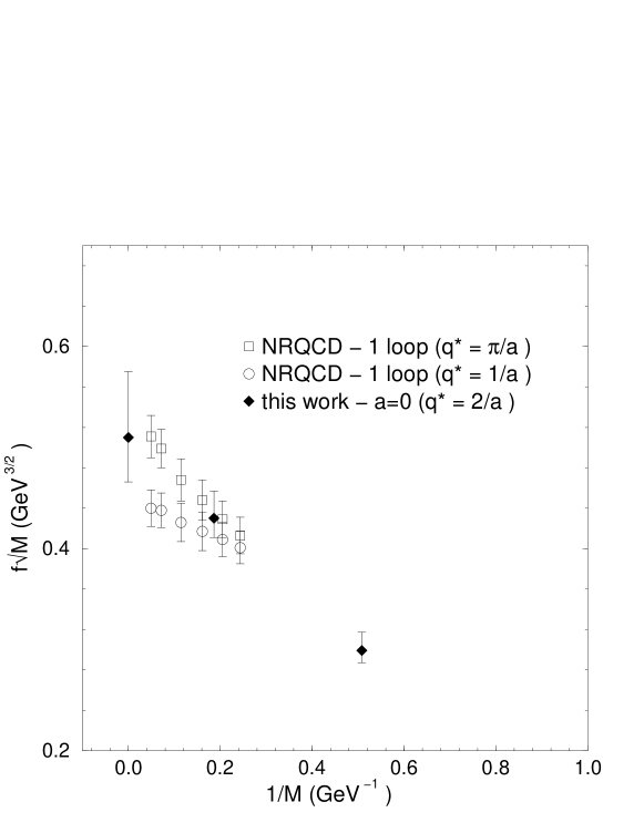
Figure 6: Comparison of the continuum limit results of this paper (filled symbols) with the results of NRQCD (open symbols). The errors shown are statistical.

As remarked earlier, for the $B$ meson system, the methods of NRQCD are also very similar to ours. This is less true for the $D$, $\psi$, and $\Upsilon$ systems. It is therefore interesting to compare recent results from the two methods. Fig. 6 shows results for $f_{M}\sqrt{M}$ as a function of $1/M$ from this paper and from a recent NRQCD calculation [28]. The NRQCD calculation includes a full ${\cal O}(a)$ correction and a full one-loop correction. This paper uses a full ${\cal O}(a)$ correction, but is missing the part of the one-loop correction arising from the ${\cal O}(a)$ correction to the current, which has not yet been calculated. The one-loop corrected results are close to each other in the region of the $B$ mass, where we have reported our main results. However, the NRQCD one-loop corrections increase greatly for larger $M$, becoming as large as $-$25% in the static limit, the result of a surprisingly large contribution from the ${\cal O}(a)$ current correction.

For all of the heavy-light decay constants, the largest source of uncertainty uncertainty, and the one under least quantitative control, is the quenched approximation. The uncertainties from all other sources of error are now less than the approximately 10% range usually associated with the quenched approximation.

Appendix A Appendix

We present in Tables 3 – 10 results for the decay constants obtained with various fitting methods. We give two tables for each of the four decay constants. The first table contains results for each of the three lattice spacings. The second table gives the results of extrapolation to the continuum limit, along with the $\chi^{2}$ of the fit. In each case, we performed the analysis with quark masses determined from the spin-averaged 1S -onium state, using one of five methods of determining the lattice spacing: the 1P–1S charmonium splitting, $f_{K}$ from either 2- or 3-state fits, or $f_{\pi}$ from either 2- or 3-state fits.

$a^{-1}$	$\beta=6.1$	$\beta=5.9$	$\beta=5.7$
1P-1S	0.511$\;\begin{array}[]{@{}l@{}}\makebox[15.0pt][c]{$+$}\makebox[3.5pt][r]{26\hfill}\\[-1.68004pt] \makebox[15.0pt][c]{$-$}\makebox[3.5pt][r]{35\hfill}\end{array}$	0.455$\;\begin{array}[]{@{}l@{}}\makebox[15.0pt][c]{$+$}\makebox[3.5pt][r]{19\hfill}\\[-1.68004pt] \makebox[15.0pt][c]{$-$}\makebox[3.5pt][r]{22\hfill}\end{array}$	0.477$\;\begin{array}[]{@{}l@{}}\makebox[15.0pt][c]{$+$}\makebox[3.5pt][r]{20\hfill}\\[-1.68004pt] \makebox[15.0pt][c]{$-$}\makebox[3.5pt][r]{22\hfill}\end{array}$
$f_{\pi}$ (2-state)	0.419$\;\begin{array}[]{@{}l@{}}\makebox[15.0pt][c]{$+$}\makebox[3.5pt][r]{37\hfill}\\[-1.68004pt] \makebox[15.0pt][c]{$-$}\makebox[3.5pt][r]{13\hfill}\end{array}$	0.407$\;\begin{array}[]{@{}l@{}}\makebox[15.0pt][c]{$+$}\makebox[3.5pt][r]{30\hfill}\\[-1.68004pt] \makebox[15.0pt][c]{$-$}\makebox[3.5pt][r]{13\hfill}\end{array}$	0.440$\;\begin{array}[]{@{}l@{}}\makebox[15.0pt][c]{$+$}\makebox[3.5pt][r]{25\hfill}\\[-1.68004pt] \makebox[15.0pt][c]{$-$}\makebox[3.5pt][r]{12\hfill}\end{array}$
$f_{\pi}$ (3-state)	0.417$\;\begin{array}[]{@{}l@{}}\makebox[15.0pt][c]{$+$}\makebox[3.5pt][r]{56\hfill}\\[-1.68004pt] \makebox[15.0pt][c]{$-$}\makebox[3.5pt][r]{38\hfill}\end{array}$	0.363$\;\begin{array}[]{@{}l@{}}\makebox[15.0pt][c]{$+$}\makebox[3.5pt][r]{21\hfill}\\[-1.68004pt] \makebox[15.0pt][c]{$-$}\makebox[3.5pt][r]{5\hfill}\end{array}$	0.384$\;\begin{array}[]{@{}l@{}}\makebox[15.0pt][c]{$+$}\makebox[3.5pt][r]{21\hfill}\\[-1.68004pt] \makebox[15.0pt][c]{$-$}\makebox[3.5pt][r]{12\hfill}\end{array}$
$f_{K}$ (2-state)	0.394$\;\begin{array}[]{@{}l@{}}\makebox[15.0pt][c]{$+$}\makebox[3.5pt][r]{25\hfill}\\[-1.68004pt] \makebox[15.0pt][c]{$-$}\makebox[3.5pt][r]{13\hfill}\end{array}$	0.371$\;\begin{array}[]{@{}l@{}}\makebox[15.0pt][c]{$+$}\makebox[3.5pt][r]{12\hfill}\\[-1.68004pt] \makebox[15.0pt][c]{$-$}\makebox[3.5pt][r]{12\hfill}\end{array}$	0.385$\;\begin{array}[]{@{}l@{}}\makebox[15.0pt][c]{$+$}\makebox[3.5pt][r]{10\hfill}\\[-1.68004pt] \makebox[15.0pt][c]{$-$}\makebox[3.5pt][r]{6\hfill}\end{array}$
$f_{K}$ (3-state)	0.391$\;\begin{array}[]{@{}l@{}}\makebox[15.0pt][c]{$+$}\makebox[3.5pt][r]{35\hfill}\\[-1.68004pt] \makebox[15.0pt][c]{$-$}\makebox[3.5pt][r]{10\hfill}\end{array}$	0.357$\;\begin{array}[]{@{}l@{}}\makebox[15.0pt][c]{$+$}\makebox[3.5pt][r]{10\hfill}\\[-1.68004pt] \makebox[15.0pt][c]{$-$}\makebox[3.5pt][r]{10\hfill}\end{array}$	0.387$\;\begin{array}[]{@{}l@{}}\makebox[15.0pt][c]{$+$}\makebox[3.5pt][r]{10\hfill}\\[-1.68004pt] \makebox[15.0pt][c]{$-$}\makebox[3.5pt][r]{7\hfill}\end{array}$

Table 3: $f_{B}\sqrt{M_{B}}$ in GeV${}^{\frac{3}{2}}$ at $\beta=6.1$, 5.9, and 5.7, fitted with the lattice spacing set in five different ways.

$a^{-1}$	$f_{B}\sqrt{M}(a=0)$	$f_{B}(a=0)$	$\chi^{2}/d.o.f$
1P-1S	0.490$\;\begin{array}[]{@{}l@{}}\makebox[15.0pt][c]{$+$}\makebox[3.5pt][r]{42\hfill}\\[-1.68004pt] \makebox[15.0pt][c]{$-$}\makebox[3.5pt][r]{51\hfill}\end{array}$	213$\;\begin{array}[]{@{}l@{}}\makebox[15.0pt][c]{$+$}\makebox[3.5pt][r]{18\hfill}\\[-1.68004pt] \makebox[15.0pt][c]{$-$}\makebox[3.5pt][r]{22\hfill}\end{array}$	2.04/1
$f_{\pi}$ (2-state)	0.386$\;\begin{array}[]{@{}l@{}}\makebox[15.0pt][c]{$+$}\makebox[3.5pt][r]{58\hfill}\\[-1.68004pt] \makebox[15.0pt][c]{$-$}\makebox[3.5pt][r]{27\hfill}\end{array}$	168$\;\begin{array}[]{@{}l@{}}\makebox[15.0pt][c]{$+$}\makebox[3.5pt][r]{25\hfill}\\[-1.68004pt] \makebox[15.0pt][c]{$-$}\makebox[3.5pt][r]{12\hfill}\end{array}$	0.51/1
$f_{\pi}$ (3-state)	0.349$\;\begin{array}[]{@{}l@{}}\makebox[15.0pt][c]{$+$}\makebox[3.5pt][r]{63\hfill}\\[-1.68004pt] \makebox[15.0pt][c]{$-$}\makebox[3.5pt][r]{33\hfill}\end{array}$	152$\;\begin{array}[]{@{}l@{}}\makebox[15.0pt][c]{$+$}\makebox[3.5pt][r]{27\hfill}\\[-1.68004pt] \makebox[15.0pt][c]{$-$}\makebox[3.5pt][r]{14\hfill}\end{array}$	1.63/1
$f_{K}$ (2-state)	0.376$\;\begin{array}[]{@{}l@{}}\makebox[15.0pt][c]{$+$}\makebox[3.5pt][r]{32\hfill}\\[-1.68004pt] \makebox[15.0pt][c]{$-$}\makebox[3.5pt][r]{25\hfill}\end{array}$	164$\;\begin{array}[]{@{}l@{}}\makebox[15.0pt][c]{$+$}\makebox[3.5pt][r]{14\hfill}\\[-1.68004pt] \makebox[15.0pt][c]{$-$}\makebox[3.5pt][r]{11\hfill}\end{array}$	1.32/1
$f_{K}$ (3-state)	0.331$\;\begin{array}[]{@{}l@{}}\makebox[15.0pt][c]{$+$}\makebox[3.5pt][r]{34\hfill}\\[-1.68004pt] \makebox[15.0pt][c]{$-$}\makebox[3.5pt][r]{24\hfill}\end{array}$	144$\;\begin{array}[]{@{}l@{}}\makebox[15.0pt][c]{$+$}\makebox[3.5pt][r]{15\hfill}\\[-1.68004pt] \makebox[15.0pt][c]{$-$}\makebox[3.5pt][r]{10\hfill}\end{array}$	3.51/1

Table 4: $f_{B}\sqrt{M_{B}}$ in GeV${}^{\frac{3}{2}}$ and $f_{B}$ in MeV extrapolated to $a=0$, fitted with the lattice spacing set in five different ways.

$a^{-1}$	$\beta=6.1$	$\beta=5.9$	$\beta=5.7$
1P-1S	0.582$\;\begin{array}[]{@{}l@{}}\makebox[15.0pt][c]{$+$}\makebox[3.5pt][r]{26\hfill}\\[-1.68004pt] \makebox[15.0pt][c]{$-$}\makebox[3.5pt][r]{32\hfill}\end{array}$	0.520$\;\begin{array}[]{@{}l@{}}\makebox[15.0pt][c]{$+$}\makebox[3.5pt][r]{21\hfill}\\[-1.68004pt] \makebox[15.0pt][c]{$-$}\makebox[3.5pt][r]{21\hfill}\end{array}$	0.545$\;\begin{array}[]{@{}l@{}}\makebox[15.0pt][c]{$+$}\makebox[3.5pt][r]{22\hfill}\\[-1.68004pt] \makebox[15.0pt][c]{$-$}\makebox[3.5pt][r]{24\hfill}\end{array}$
$f_{\pi}$ (2-state)	0.478$\;\begin{array}[]{@{}l@{}}\makebox[15.0pt][c]{$+$}\makebox[3.5pt][r]{36\hfill}\\[-1.68004pt] \makebox[15.0pt][c]{$-$}\makebox[3.5pt][r]{10\hfill}\end{array}$	0.465$\;\begin{array}[]{@{}l@{}}\makebox[15.0pt][c]{$+$}\makebox[3.5pt][r]{33\hfill}\\[-1.68004pt] \makebox[15.0pt][c]{$-$}\makebox[3.5pt][r]{11\hfill}\end{array}$	0.503$\;\begin{array}[]{@{}l@{}}\makebox[15.0pt][c]{$+$}\makebox[3.5pt][r]{27\hfill}\\[-1.68004pt] \makebox[15.0pt][c]{$-$}\makebox[3.5pt][r]{13\hfill}\end{array}$
$f_{\pi}$ (3-state)	0.476$\;\begin{array}[]{@{}l@{}}\makebox[15.0pt][c]{$+$}\makebox[3.5pt][r]{60\hfill}\\[-1.68004pt] \makebox[15.0pt][c]{$-$}\makebox[3.5pt][r]{41\hfill}\end{array}$	0.415$\;\begin{array}[]{@{}l@{}}\makebox[15.0pt][c]{$+$}\makebox[3.5pt][r]{22\hfill}\\[-1.68004pt] \makebox[15.0pt][c]{$-$}\makebox[3.5pt][r]{2\hfill}\end{array}$	0.439$\;\begin{array}[]{@{}l@{}}\makebox[15.0pt][c]{$+$}\makebox[3.5pt][r]{23\hfill}\\[-1.68004pt] \makebox[15.0pt][c]{$-$}\makebox[3.5pt][r]{12\hfill}\end{array}$
$f_{K}$ (2-state)	0.449$\;\begin{array}[]{@{}l@{}}\makebox[15.0pt][c]{$+$}\makebox[3.5pt][r]{23\hfill}\\[-1.68004pt] \makebox[15.0pt][c]{$-$}\makebox[3.5pt][r]{10\hfill}\end{array}$	0.424$\;\begin{array}[]{@{}l@{}}\makebox[15.0pt][c]{$+$}\makebox[3.5pt][r]{12\hfill}\\[-1.68004pt] \makebox[15.0pt][c]{$-$}\makebox[3.5pt][r]{9\hfill}\end{array}$	0.440$\;\begin{array}[]{@{}l@{}}\makebox[15.0pt][c]{$+$}\makebox[3.5pt][r]{11\hfill}\\[-1.68004pt] \makebox[15.0pt][c]{$-$}\makebox[3.5pt][r]{6\hfill}\end{array}$
$f_{K}$ (3-state)	0.445$\;\begin{array}[]{@{}l@{}}\makebox[15.0pt][c]{$+$}\makebox[3.5pt][r]{32\hfill}\\[-1.68004pt] \makebox[15.0pt][c]{$-$}\makebox[3.5pt][r]{7\hfill}\end{array}$	0.408$\;\begin{array}[]{@{}l@{}}\makebox[15.0pt][c]{$+$}\makebox[3.5pt][r]{8\hfill}\\[-1.68004pt] \makebox[15.0pt][c]{$-$}\makebox[3.5pt][r]{5\hfill}\end{array}$	0.442$\;\begin{array}[]{@{}l@{}}\makebox[15.0pt][c]{$+$}\makebox[3.5pt][r]{10\hfill}\\[-1.68004pt] \makebox[15.0pt][c]{$-$}\makebox[3.5pt][r]{6\hfill}\end{array}$

Table 5: $f_{B_{s}}\sqrt{M_{B_{s}}}$ in GeV${}^{\frac{3}{2}}$ at $\beta=6.1$, 5.9, and 5.7, fitted with the lattice spacing set in five different ways.

$a^{-1}$	$f_{B_{s}}\sqrt{M}(a=0)$	$f_{B_{s}}(a=0)$	$\chi^{2}/d.o.f$
1P-1S	0.567$\;\begin{array}[]{@{}l@{}}\makebox[15.0pt][c]{$+$}\makebox[3.5pt][r]{42\hfill}\\[-1.68004pt] \makebox[15.0pt][c]{$-$}\makebox[3.5pt][r]{50\hfill}\end{array}$	244$\;\begin{array}[]{@{}l@{}}\makebox[15.0pt][c]{$+$}\makebox[3.5pt][r]{18\hfill}\\[-1.68004pt] \makebox[15.0pt][c]{$-$}\makebox[3.5pt][r]{22\hfill}\end{array}$	2.80/1
$f_{\pi}$ (2-state)	0.444$\;\begin{array}[]{@{}l@{}}\makebox[15.0pt][c]{$+$}\makebox[3.5pt][r]{61\hfill}\\[-1.68004pt] \makebox[15.0pt][c]{$-$}\makebox[3.5pt][r]{22\hfill}\end{array}$	192$\;\begin{array}[]{@{}l@{}}\makebox[15.0pt][c]{$+$}\makebox[3.5pt][r]{26\hfill}\\[-1.68004pt] \makebox[15.0pt][c]{$-$}\makebox[3.5pt][r]{10\hfill}\end{array}$	0.59/1
$f_{\pi}$ (3-state)	0.395$\;\begin{array}[]{@{}l@{}}\makebox[15.0pt][c]{$+$}\makebox[3.5pt][r]{68\hfill}\\[-1.68004pt] \makebox[15.0pt][c]{$-$}\makebox[3.5pt][r]{31\hfill}\end{array}$	170$\;\begin{array}[]{@{}l@{}}\makebox[15.0pt][c]{$+$}\makebox[3.5pt][r]{29\hfill}\\[-1.68004pt] \makebox[15.0pt][c]{$-$}\makebox[3.5pt][r]{13\hfill}\end{array}$	1.81/1
$f_{K}$ (2-state)	0.430$\;\begin{array}[]{@{}l@{}}\makebox[15.0pt][c]{$+$}\makebox[3.5pt][r]{29\hfill}\\[-1.68004pt] \makebox[15.0pt][c]{$-$}\makebox[3.5pt][r]{19\hfill}\end{array}$	185$\;\begin{array}[]{@{}l@{}}\makebox[15.0pt][c]{$+$}\makebox[3.5pt][r]{13\hfill}\\[-1.68004pt] \makebox[15.0pt][c]{$-$}\makebox[3.5pt][r]{8\hfill}\end{array}$	2.06/1
$f_{K}$ (3-state)	0.374$\;\begin{array}[]{@{}l@{}}\makebox[15.0pt][c]{$+$}\makebox[3.5pt][r]{31\hfill}\\[-1.68004pt] \makebox[15.0pt][c]{$-$}\makebox[3.5pt][r]{20\hfill}\end{array}$	161$\;\begin{array}[]{@{}l@{}}\makebox[15.0pt][c]{$+$}\makebox[3.5pt][r]{14\hfill}\\[-1.68004pt] \makebox[15.0pt][c]{$-$}\makebox[3.5pt][r]{9\hfill}\end{array}$	6.51/1

Table 6: $f_{B_{s}}\sqrt{M_{B_{s}}}$ in GeV${}^{\frac{3}{2}}$ and $f_{B_{s}}$ in MeV extrapolated to $a=0$, fitted with the lattice spacing set in five different ways.

$a^{-1}$	$\beta=6.1$	$\beta=5.9$	$\beta=5.7$
1P-1S	0.332$\;\begin{array}[]{@{}l@{}}\makebox[15.0pt][c]{$+$}\makebox[3.5pt][r]{16\hfill}\\[-1.68004pt] \makebox[15.0pt][c]{$-$}\makebox[3.5pt][r]{23\hfill}\end{array}$	0.329$\;\begin{array}[]{@{}l@{}}\makebox[15.0pt][c]{$+$}\makebox[3.5pt][r]{13\hfill}\\[-1.68004pt] \makebox[15.0pt][c]{$-$}\makebox[3.5pt][r]{15\hfill}\end{array}$	0.323$\;\begin{array}[]{@{}l@{}}\makebox[15.0pt][c]{$+$}\makebox[3.5pt][r]{13\hfill}\\[-1.68004pt] \makebox[15.0pt][c]{$-$}\makebox[3.5pt][r]{15\hfill}\end{array}$
$f_{\pi}$ (2-state)	0.273$\;\begin{array}[]{@{}l@{}}\makebox[15.0pt][c]{$+$}\makebox[3.5pt][r]{23\hfill}\\[-1.68004pt] \makebox[15.0pt][c]{$-$}\makebox[3.5pt][r]{9\hfill}\end{array}$	0.294$\;\begin{array}[]{@{}l@{}}\makebox[15.0pt][c]{$+$}\makebox[3.5pt][r]{20\hfill}\\[-1.68004pt] \makebox[15.0pt][c]{$-$}\makebox[3.5pt][r]{9\hfill}\end{array}$	0.298$\;\begin{array}[]{@{}l@{}}\makebox[15.0pt][c]{$+$}\makebox[3.5pt][r]{15\hfill}\\[-1.68004pt] \makebox[15.0pt][c]{$-$}\makebox[3.5pt][r]{8\hfill}\end{array}$
$f_{\pi}$ (3-state)	0.271$\;\begin{array}[]{@{}l@{}}\makebox[15.0pt][c]{$+$}\makebox[3.5pt][r]{35\hfill}\\[-1.68004pt] \makebox[15.0pt][c]{$-$}\makebox[3.5pt][r]{24\hfill}\end{array}$	0.262$\;\begin{array}[]{@{}l@{}}\makebox[15.0pt][c]{$+$}\makebox[3.5pt][r]{13\hfill}\\[-1.68004pt] \makebox[15.0pt][c]{$-$}\makebox[3.5pt][r]{2\hfill}\end{array}$	0.261$\;\begin{array}[]{@{}l@{}}\makebox[15.0pt][c]{$+$}\makebox[3.5pt][r]{13\hfill}\\[-1.68004pt] \makebox[15.0pt][c]{$-$}\makebox[3.5pt][r]{8\hfill}\end{array}$
$f_{K}$ (2-state)	0.256$\;\begin{array}[]{@{}l@{}}\makebox[15.0pt][c]{$+$}\makebox[3.5pt][r]{15\hfill}\\[-1.68004pt] \makebox[15.0pt][c]{$-$}\makebox[3.5pt][r]{8\hfill}\end{array}$	0.268$\;\begin{array}[]{@{}l@{}}\makebox[15.0pt][c]{$+$}\makebox[3.5pt][r]{8\hfill}\\[-1.68004pt] \makebox[15.0pt][c]{$-$}\makebox[3.5pt][r]{7\hfill}\end{array}$	0.261$\;\begin{array}[]{@{}l@{}}\makebox[15.0pt][c]{$+$}\makebox[3.5pt][r]{5\hfill}\\[-1.68004pt] \makebox[15.0pt][c]{$-$}\makebox[3.5pt][r]{4\hfill}\end{array}$
$f_{K}$ (3-state)	0.254$\;\begin{array}[]{@{}l@{}}\makebox[15.0pt][c]{$+$}\makebox[3.5pt][r]{21\hfill}\\[-1.68004pt] \makebox[15.0pt][c]{$-$}\makebox[3.5pt][r]{7\hfill}\end{array}$	0.258$\;\begin{array}[]{@{}l@{}}\makebox[15.0pt][c]{$+$}\makebox[3.5pt][r]{5\hfill}\\[-1.68004pt] \makebox[15.0pt][c]{$-$}\makebox[3.5pt][r]{4\hfill}\end{array}$	0.262$\;\begin{array}[]{@{}l@{}}\makebox[15.0pt][c]{$+$}\makebox[3.5pt][r]{5\hfill}\\[-1.68004pt] \makebox[15.0pt][c]{$-$}\makebox[3.5pt][r]{4\hfill}\end{array}$

Table 7: $f_{D}\sqrt{M_{D}}$ in GeV${}^{\frac{3}{2}}$ at $\beta=6.1$, 5.9, and 5.7, fitted with the lattice spacing set in five different ways.

$a^{-1}$	$f_{D}\sqrt{M}(a=0)$	$f_{D}(a=0)$	$\chi^{2}/d.o.f$
1P-1S	0.339$\;\begin{array}[]{@{}l@{}}\makebox[15.0pt][c]{$+$}\makebox[3.5pt][r]{27\hfill}\\[-1.68004pt] \makebox[15.0pt][c]{$-$}\makebox[3.5pt][r]{34\hfill}\end{array}$	248$\;\begin{array}[]{@{}l@{}}\makebox[15.0pt][c]{$+$}\makebox[3.5pt][r]{20\hfill}\\[-1.68004pt] \makebox[15.0pt][c]{$-$}\makebox[3.5pt][r]{24\hfill}\end{array}$	0.03/1
$f_{\pi}$ (2-state)	0.262$\;\begin{array}[]{@{}l@{}}\makebox[15.0pt][c]{$+$}\makebox[3.5pt][r]{38\hfill}\\[-1.68004pt] \makebox[15.0pt][c]{$-$}\makebox[3.5pt][r]{18\hfill}\end{array}$	191$\;\begin{array}[]{@{}l@{}}\makebox[15.0pt][c]{$+$}\makebox[3.5pt][r]{28\hfill}\\[-1.68004pt] \makebox[15.0pt][c]{$-$}\makebox[3.5pt][r]{13\hfill}\end{array}$	0.43/1
$f_{\pi}$ (3-state)	0.268$\;\begin{array}[]{@{}l@{}}\makebox[15.0pt][c]{$+$}\makebox[3.5pt][r]{39\hfill}\\[-1.68004pt] \makebox[15.0pt][c]{$-$}\makebox[3.5pt][r]{20\hfill}\end{array}$	196$\;\begin{array}[]{@{}l@{}}\makebox[15.0pt][c]{$+$}\makebox[3.5pt][r]{29\hfill}\\[-1.68004pt] \makebox[15.0pt][c]{$-$}\makebox[3.5pt][r]{15\hfill}\end{array}$	0.06/1
$f_{K}$ (2-state)	0.265$\;\begin{array}[]{@{}l@{}}\makebox[15.0pt][c]{$+$}\makebox[3.5pt][r]{19\hfill}\\[-1.68004pt] \makebox[15.0pt][c]{$-$}\makebox[3.5pt][r]{14\hfill}\end{array}$	194$\;\begin{array}[]{@{}l@{}}\makebox[15.0pt][c]{$+$}\makebox[3.5pt][r]{14\hfill}\\[-1.68004pt] \makebox[15.0pt][c]{$-$}\makebox[3.5pt][r]{10\hfill}\end{array}$	0.77/1
$f_{K}$ (3-state)	0.249$\;\begin{array}[]{@{}l@{}}\makebox[15.0pt][c]{$+$}\makebox[3.5pt][r]{15\hfill}\\[-1.68004pt] \makebox[15.0pt][c]{$-$}\makebox[3.5pt][r]{13\hfill}\end{array}$	182$\;\begin{array}[]{@{}l@{}}\makebox[15.0pt][c]{$+$}\makebox[3.5pt][r]{11\hfill}\\[-1.68004pt] \makebox[15.0pt][c]{$-$}\makebox[3.5pt][r]{10\hfill}\end{array}$	0.01/1

Table 8: $f_{D}\sqrt{M_{D}}$ in GeV${}^{\frac{3}{2}}$ and $f_{D}$ in MeV extrapolated to $a=0$, fitted with the lattice spacing set in five different ways.

$a^{-1}$	$\beta=6.1$	$\beta=5.9$	$\beta=5.7$
1P-1S	0.380$\;\begin{array}[]{@{}l@{}}\makebox[15.0pt][c]{$+$}\makebox[3.5pt][r]{16\hfill}\\[-1.68004pt] \makebox[15.0pt][c]{$-$}\makebox[3.5pt][r]{22\hfill}\end{array}$	0.376$\;\begin{array}[]{@{}l@{}}\makebox[15.0pt][c]{$+$}\makebox[3.5pt][r]{15\hfill}\\[-1.68004pt] \makebox[15.0pt][c]{$-$}\makebox[3.5pt][r]{15\hfill}\end{array}$	0.372$\;\begin{array}[]{@{}l@{}}\makebox[15.0pt][c]{$+$}\makebox[3.5pt][r]{15\hfill}\\[-1.68004pt] \makebox[15.0pt][c]{$-$}\makebox[3.5pt][r]{16\hfill}\end{array}$
$f_{\pi}$ (2-state)	0.312$\;\begin{array}[]{@{}l@{}}\makebox[15.0pt][c]{$+$}\makebox[3.5pt][r]{24\hfill}\\[-1.68004pt] \makebox[15.0pt][c]{$-$}\makebox[3.5pt][r]{8\hfill}\end{array}$	0.336$\;\begin{array}[]{@{}l@{}}\makebox[15.0pt][c]{$+$}\makebox[3.5pt][r]{24\hfill}\\[-1.68004pt] \makebox[15.0pt][c]{$-$}\makebox[3.5pt][r]{8\hfill}\end{array}$	0.343$\;\begin{array}[]{@{}l@{}}\makebox[15.0pt][c]{$+$}\makebox[3.5pt][r]{18\hfill}\\[-1.68004pt] \makebox[15.0pt][c]{$-$}\makebox[3.5pt][r]{9\hfill}\end{array}$
$f_{\pi}$ (3-state)	0.310$\;\begin{array}[]{@{}l@{}}\makebox[15.0pt][c]{$+$}\makebox[3.5pt][r]{40\hfill}\\[-1.68004pt] \makebox[15.0pt][c]{$-$}\makebox[3.5pt][r]{25\hfill}\end{array}$	0.300$\;\begin{array}[]{@{}l@{}}\makebox[15.0pt][c]{$+$}\makebox[3.5pt][r]{15\hfill}\\[-1.68004pt] \makebox[15.0pt][c]{$-$}\makebox[3.5pt][r]{1\hfill}\end{array}$	0.300$\;\begin{array}[]{@{}l@{}}\makebox[15.0pt][c]{$+$}\makebox[3.5pt][r]{16\hfill}\\[-1.68004pt] \makebox[15.0pt][c]{$-$}\makebox[3.5pt][r]{8\hfill}\end{array}$
$f_{K}$ (2-state)	0.293$\;\begin{array}[]{@{}l@{}}\makebox[15.0pt][c]{$+$}\makebox[3.5pt][r]{15\hfill}\\[-1.68004pt] \makebox[15.0pt][c]{$-$}\makebox[3.5pt][r]{7\hfill}\end{array}$	0.306$\;\begin{array}[]{@{}l@{}}\makebox[15.0pt][c]{$+$}\makebox[3.5pt][r]{9\hfill}\\[-1.68004pt] \makebox[15.0pt][c]{$-$}\makebox[3.5pt][r]{6\hfill}\end{array}$	0.301$\;\begin{array}[]{@{}l@{}}\makebox[15.0pt][c]{$+$}\makebox[3.5pt][r]{7\hfill}\\[-1.68004pt] \makebox[15.0pt][c]{$-$}\makebox[3.5pt][r]{3\hfill}\end{array}$
$f_{K}$ (3-state)	0.290$\;\begin{array}[]{@{}l@{}}\makebox[15.0pt][c]{$+$}\makebox[3.5pt][r]{23\hfill}\\[-1.68004pt] \makebox[15.0pt][c]{$-$}\makebox[3.5pt][r]{5\hfill}\end{array}$	0.295$\;\begin{array}[]{@{}l@{}}\makebox[15.0pt][c]{$+$}\makebox[3.5pt][r]{5\hfill}\\[-1.68004pt] \makebox[15.0pt][c]{$-$}\makebox[3.5pt][r]{3\hfill}\end{array}$	0.302$\;\begin{array}[]{@{}l@{}}\makebox[15.0pt][c]{$+$}\makebox[3.5pt][r]{6\hfill}\\[-1.68004pt] \makebox[15.0pt][c]{$-$}\makebox[3.5pt][r]{3\hfill}\end{array}$

Table 9: $f_{D_{s}}\sqrt{M_{D_{s}}}$ in GeV${}^{\frac{3}{2}}$ at $\beta=6.1$, 5.9, and 5.7, fitted with the lattice spacing set in five different ways.

$a^{-1}$	$f_{D_{s}}\sqrt{M}(a=0)$	$f_{D_{s}}(a=0)$	$\chi^{2}/d.o.f$
1P-1S	0.384$\;\begin{array}[]{@{}l@{}}\makebox[15.0pt][c]{$+$}\makebox[3.5pt][r]{31\hfill}\\[-1.68004pt] \makebox[15.0pt][c]{$-$}\makebox[3.5pt][r]{35\hfill}\end{array}$	274$\;\begin{array}[]{@{}l@{}}\makebox[15.0pt][c]{$+$}\makebox[3.5pt][r]{22\hfill}\\[-1.68004pt] \makebox[15.0pt][c]{$-$}\makebox[3.5pt][r]{25\hfill}\end{array}$	0.01/1
$f_{\pi}$ (2-state)	0.295$\;\begin{array}[]{@{}l@{}}\makebox[15.0pt][c]{$+$}\makebox[3.5pt][r]{39\hfill}\\[-1.68004pt] \makebox[15.0pt][c]{$-$}\makebox[3.5pt][r]{16\hfill}\end{array}$	210$\;\begin{array}[]{@{}l@{}}\makebox[15.0pt][c]{$+$}\makebox[3.5pt][r]{28\hfill}\\[-1.68004pt] \makebox[15.0pt][c]{$-$}\makebox[3.5pt][r]{11\hfill}\end{array}$	0.42/1
$f_{\pi}$ (3-state)	0.303$\;\begin{array}[]{@{}l@{}}\makebox[15.0pt][c]{$+$}\makebox[3.5pt][r]{46\hfill}\\[-1.68004pt] \makebox[15.0pt][c]{$-$}\makebox[3.5pt][r]{20\hfill}\end{array}$	216$\;\begin{array}[]{@{}l@{}}\makebox[15.0pt][c]{$+$}\makebox[3.5pt][r]{33\hfill}\\[-1.68004pt] \makebox[15.0pt][c]{$-$}\makebox[3.5pt][r]{14\hfill}\end{array}$	0.08/1
$f_{K}$ (2-state)	0.299$\;\begin{array}[]{@{}l@{}}\makebox[15.0pt][c]{$+$}\makebox[3.5pt][r]{19\hfill}\\[-1.68004pt] \makebox[15.0pt][c]{$-$}\makebox[3.5pt][r]{15\hfill}\end{array}$	213$\;\begin{array}[]{@{}l@{}}\makebox[15.0pt][c]{$+$}\makebox[3.5pt][r]{14\hfill}\\[-1.68004pt] \makebox[15.0pt][c]{$-$}\makebox[3.5pt][r]{11\hfill}\end{array}$	1.01/1
$f_{K}$ (3-state)	0.281$\;\begin{array}[]{@{}l@{}}\makebox[15.0pt][c]{$+$}\makebox[3.5pt][r]{17\hfill}\\[-1.68004pt] \makebox[15.0pt][c]{$-$}\makebox[3.5pt][r]{11\hfill}\end{array}$	201$\;\begin{array}[]{@{}l@{}}\makebox[15.0pt][c]{$+$}\makebox[3.5pt][r]{12\hfill}\\[-1.68004pt] \makebox[15.0pt][c]{$-$}\makebox[3.5pt][r]{8\hfill}\end{array}$	0.10/1

Table 10: $f_{D_{s}}\sqrt{M_{D_{s}}}$ in GeV${}^{\frac{3}{2}}$ and $f_{D_{s}}$ in MeV extrapolated to $a=0$, fitted with the lattice spacing set in five different ways.

References

• [1] C. Bernard, Nucl. Phys. B Proc. Suppl. 34 (1994) 47.
• [2] E. Eichten, Nucl. Phys. B Proc. Suppl. 20 (1994) 475.
• [3] W. E. Caswell and G. P. Lepage, Phys. Lett. 167B (1986) 437.
• [4] G. P. Lepage and B. A. Thacker, Nucl. Phys. B Proc. Suppl. 4 (1987) 199;
B. A. Thacker and G. P. Lepage, Phys. Rev. D43 (1991) 196.
• [5] G. P. Lepage, L. Magnea, C. Nakhleh, U. Magnea, and K. Hornbostel, Phys. Rev. D46 (1992) 4052.
• [6] E. Eichten, Nucl. Phys. B Proc. Suppl. 4 (1987) 170.
• [7] E. Eichten and B. Hill, Phys. Lett. B243 (1990) 427.
• [8] A. X. El-Khadra, A. S. Kronfeld, P. B. Mackenzie, Phys. Rev. D55 (1997) 3933.
• [9] P.B. Mackenzie, Nucl. Phys. B Proc. Suppl. 30 (1993) 35; A.S. Kronfeld, Nucl. Phys. B Proc. Suppl. 30 (1993) 445.
• [10] K.G. Wilson, Phys. Rev. D10 (1974) 2445; K.G. Wilson, in New Phenomena in Subnuclear Physics, edited by A. Zichichi (Plenum, New York, 1977).
• [11] B. Sheikholeslami and R. Wohlert, Nucl. Phys. B259 (1985) 572.
• [12] G.P. Lepage and P.B. Mackenzie, Phys. Rev. D48 (1993) 2250.
• [13] A.S. Kronfeld and B.P. Mertens, Nucl. Phys. B Proc. Suppl. 34 (1994) 495; B. P. Mertens et al., in preparation.
• [14] Y.Kuramashi, Perturbative Renormalization Factors of Bilinear Operators for Massive Wilson Quarks on the Lattice, KEK-CP-55 (May 1997) [hep-lat 9705036].
• [15] S. Aoki, S. Hashimoto, K. I. Ishikawa, T. Onogi, in preparation.
• [16] S. Hashimoto, private communication.
• [17] B. J. Gough et al., Phys. Rev. Lett. 79 (1997) 1622, hep-ph 9610223.
• [18] S. Ryan and J. Simone, to appear in the proceedings of Lattice 97, FNAL Conf-97/348-T.
• [19] C. Bernard et al., Heavy Light Decay Constants From Wilson and Static Quarks, to appear in the proceedings of Lattice 97. hep-lat/9709142; C. Bernard et al., $B$ Mixing on the Lattice: $f_{B}$, $f_{B_{s}}$, and Related Quantities, hep-lat/9709328.
• [20] J. Richman, Proc. ICHEP96, 28th Int. Conf. on High Energy Physics, ed. by Z. Ajduk and A. K. Wroblewski, World Scientific, Singapore (1997) 143, hep-ex/9701014 .
• [21] B. Grinstein, Phys. Rev. Lett. 71 9701014 (1993) 3067.
• [22] T. Onogi, Semileptonic Form Factors, to appear in the proceedings of Lattice 97.
• [23] A. Ali Khan, $f_{B}$ and the Heavy-light Spectrum from NRQCD, hep-lat 9710087, to appear in the proceedings of Lattice 97.
• [24] H. Wittig, Leptonic Decays of Heavy Quarks on the Lattice. OUTP-97-20-P, May 1997, hep-lat 9705034.
• [25] C. Bernard, Lattice Calculations of Decay Constants, hep-ph/9709460.
• [26] S. Aoki et al., B Meson Decay Constant and Nonrelativistic Interpretation of Wilson and Clover Fermion Actions for Heavy Quark. KEK-CP-061 (Aug 1997); S. Aoki et al., to appear.
• [27] C.R. Allton et al., Phys. Lett. B405 (1997) 133.
• [28] J. Shigemitsu, B Meson Decay Constants Using NRQCD, OHSTPY-HEP-T-97-007 (Mar 1997) hep-lat 9705017; A. Ali Khan et al., to be published in Phys. Rev. D, hep-lat 9704008; A. Ali Khan et al., OHSTPY-HEP-T-97-017, to appear.