ISU-HET-97-6

October, 1997

Long Distance Contribution to $K_{L}\rightarrow\ell^{+}\ell^{-}$

G. Valencia
Department of Physics and Astronomy
Iowa State University
Ames IA 50011
e-mail:valencia@iastate.edu

We revisit the calculation of the long distance contribution to $K_{L}\rightarrow\mu^{+}\mu^{-}$. We discuss this process within the framework of chiral perturbation theory, and also using simple models for the $K_{L}\gamma^{*}\gamma^{*}$ vertex. We argue that it is unlikely that this mode can be used to extract information on short distance parameters. The process $K_{L}\rightarrow e^{+}e^{-}$ is also long-distance dominated and we find that $B(K_{L}\rightarrow e^{+}e^{-})\approx 9\times 10^{-12}$.

1 Introduction

The rare decay mode $K_{L}\rightarrow\mu^{+}\mu^{-}$ has been the subject of many discussions [1, 2, 3, 4, 5, 6]. The current interest in this mode arises because experiment E871 at Brookhaven National Laboratory expects to collect a sample of about $10^{4}$ events [5]. Theoretically, the interest in this decay mode focuses almost exclusively in the possibility of extracting constraints on $\rho$ in the Wolfenstein parameterization of the CKM matrix.

The measured rate can be attributed to the sum of an absorptive part arising from a two-photon intermediate state, and a real part arising from the coherent sum of the dispersive contribution of the two photon intermediate state and a short distance contribution that depends on $\rho$. Therefore, to extract information on $\rho$, one must be able to calculate reliably the dispersive contribution associated with the two photon intermediate state.

The short distance contribution to this process has been known for quite some time [1, 8]. A recent review that presents all the relevant details of the status of this calculation is Ref. [9]. For our purposes it will suffice to quote an approximate result for $m_{t}=175$ GeV and $V_{cb}=0.040$ [10]:

$$B(K_{L}\rightarrow\mu^{+}\mu^{-})_{SD}=7.9\times 10^{-10}(\rho_{0}-\rho)^{2}$$ (1)

$\rho_{0}\sim 1.2$ is a measure of the charm-quark contribution to this decay.

In order to discuss the two-photon contribution, it is convenient to normalize the decay rate to the two-photon mode. Using the notation $\beta_{\ell}\equiv\sqrt{1-4m_{\ell}^{2}/M_{K}^{2}}$ we have:

$${B(K_{L}\rightarrow\ell^{+}\ell^{-})\over B(K_{L}\rightarrow\gamma\gamma)}=2\biggl{(}{m_{\ell}\over M_{K}}\biggr{)}^{2}\biggl{(}{\alpha_{em}\over\pi}\biggr{)}^{2}\beta_{\ell}\biggl{[}({\rm Re}A)^{2}+({\rm Im}A)^{2}\biggr{]},$$ (2)

The absorptive contribution to the rate is determined uniquely, it corresponds to:

$${\rm Im}A={\pi\over 2\beta_{\ell}}\log\biggl{(}{1+\beta_{\ell}\over 1-\beta_{\ell}}\biggr{)}.$$ (3)

If we use the branching ratio quoted in the Particle Data Book [11]:

$$B(K_{L}\rightarrow\gamma\gamma)=(5.92\pm 0.15)\times 10^{-4}$$ (4)

we find that the absorptive part of the two-photon contribution to $K_{L}\rightarrow\mu^{+}\mu^{-}$ is:

$$B(K_{L}\rightarrow\mu^{+}\mu^{-})_{\rm ABS}=(7.1\pm 0.2)\times 10^{-9}.$$ (5)

At the same time, the rate for $K_{L}\rightarrow\mu^{+}\mu^{-}$ has been measured to be:

$$B(K_{L}\rightarrow\mu^{+}\mu^{-})=\cases{(7.2\pm 0.5)\times 10^{-9}&PDB \cite[cite]{[\@@bibref{}{pdb}{}{}]}\cr(6.86\pm 0.37)\times 10^{-9}&AGS-791 \cite[cite]{[\@@bibref{}{heinson}{}{}]}\cr(7.9\pm 0.7)\times 10^{-9}&KEK 137 \cite[cite]{[\@@bibref{}{mumu137}{}{}]}\cr}$$ (6)

If we use, for definiteness, the Particle Data Book average, we find that the absorptive part almost completely saturates the experimental rate and that there is room for a small real part in the amplitude (arising from the coherent sum of the short distance and two-photon dispersive contributions). Taking into account that the total rate must be greater than or equal to the absorptive contribution, we can write:

$${\rm Re}A=0\pm 1.2$$ (7)

There exist several models in the literature that allow one to estimate the size of the long distance two-photon contribution. However, these models do not provide a reliable estimate of the uncertainty in their predictions. Nevertheless, a recent paper [14] claims to obtain a reliable estimate of the magnitude and uncertainty of the two-photon contribution and from this a lower bound on $\rho$.

In this paper we revisit the issue of the two-photon long distance contribution to $K_{L}\rightarrow\mu^{+}\mu^{-}$. We first use the framework of chiral perturbation theory to parameterize the dispersive part of the two-photon contribution in terms of one unknown combination of constants. We argue that this combination cannot be measured in any other process and, therefore, that it is not possible to remove the uncertainty. We then turn our attention to a simple pole model for the $K_{L}\gamma^{*}\gamma^{*}$ vertex that we use to discuss some of the model calculations that have appeared in the literature and to offer an estimate for the uncertainty of the result. Finally, we discuss a slightly more complicated model that illustrates why a more precise measurement of the decay parameters in $K_{L}\rightarrow\ell^{+}\ell^{-}\gamma$ will not reduce the uncertainty in the dispersive two-photon contribution to $K_{L}\rightarrow\ell^{+}\ell^{-}$. We conclude that it is not possible at present to extract information on the short distance parameter $\rho$ from the measurement of $K_{L}\rightarrow\mu^{+}\mu^{-}$.

2 Chiral Perturbation Theory

To calculate the dispersive part of the two-photon intermediate state it is not sufficient to know the $K_{L}\rightarrow\gamma\gamma$ amplitude on shell, so we parameterize the $K_{L}\gamma^{*}\gamma^{*}$ vertex in the following way:

$$\Gamma^{\mu\nu}(q_{1},q_{2})=2{\alpha_{em}\over\pi}G_{8}f_{\pi}F(q_{1}^{2},q_{2}^{2})\epsilon_{\alpha\beta\mu\nu}q_{1}^{\alpha}q_{2}^{\beta}.$$ (8)

The overall constant, with $G_{8}\approx 5.1G_{F}/\sqrt{2}|V_{ud}V^{*}_{us}|$, has been chosen for convenience [6]. With this normalization, the measured rate for $K_{L}\rightarrow\gamma\gamma$, Eq. 4, implies the value

$$F_{1}\equiv F(0,0)=0.90\pm 0.01$$ (9)

The behavior of the vertex $\Gamma^{\mu\nu}(q_{1},q_{2})$ (Eq. 8) as a function of $q_{1}^{2}$ and $q_{2}^{2}$ is described by the function $F(q_{1}^{2},q_{2}^{2})$. This function is symmetric under the interchange $q_{1}\leftrightarrow q_{2}$ due to Bose symmetry. For energies that are small compared to the scale of chiral symmetry breaking, $\Lambda\sim 1$ GeV, we find it convenient to write this form factor as:

$$F(q_{1}^{2},q_{2}^{2})=F(0,0)\biggl{(}1+\alpha{(q_{1}^{2}+q_{2}^{2})\over\Lambda^{2}}+\beta{(q_{1}^{4}+q_{2}^{4})\over\Lambda^{4}}+\beta^{\prime}{q_{1}^{2}q_{2}^{2}\over\Lambda^{4}}+\cdots\biggr{)}$$ (10)

It should be possible to extract the first few parameters in this expansion from measurements in the modes $K_{L}\rightarrow\ell^{+}\ell^{-}\gamma$. In fact, a study of $K_{L}\rightarrow e^{+}e^{-}\gamma$ has already found [15]

$$\alpha=3.15\pm 0.40.$$ (11)

Measurements of $K_{L}\rightarrow\mu^{+}\mu^{-}\gamma$ are consistent with this number at the two standard deviation level [16]. It should be possible to improve the precision of this number, as well as to measure the parameters $\beta$ and $\beta^{\prime}$ in the current generation of experiments. In this regard, it is important to emphasize that it would be valuable to have a direct fit to these parameters from the experiments, instead of the fit to the parameter $\alpha_{K^{*}}$ that is currently performed. This was already suggested in References [6] and [14].

The measured values of $F_{1}$ and $\alpha$, justify the way we wrote the low energy expansion in Eq. 10. However, in chiral perturbation theory one finds that $F(q_{1}^{2},q_{2}^{2})$ vanishes at order $p^{4}$ [17]. The leading contributions appear at order $p^{6}$, and this implies that, formally, $F_{1}$ and $\alpha$ are of the same order. To be truly consistent with $\chi$PT we should write $M_{K}^{2}/\Lambda^{2}$ instead of one in the first term of Eq. 10. As we will see, this complicates the discussion without altering the conclusions, so we leave Eq. 10 as it stands.

Let us first evaluate the one-loop, two-photon intermediate state, contribution to $K_{L}\rightarrow\ell^{+}\ell^{-}$. To leading order in $\chi$PT, the contribution of this loop is obtained by using the vertex of Eq. 8 with the form factor of Eq. 10 truncated at the term linear in $q_{i}^{2}$, and attaching the photons to the leptons with the usual rules of QED. The resulting one-loop diagram is divergent and the calculation of the physical process requires local counter-terms.

The local counter-terms are written as a chiral Lagrangian using standard notation [18]. The pion and kaon fields are identified with the Goldstone bosons of the spontaneously broken $SU(3)_{L}\times SU(3)_{R}$ chiral symmetry and are incorporated via the matrix:

$$\phi = {1\over\sqrt{2}}\left(\begin{array}[]{ccc}\pi^{0}/\sqrt{2}+\eta/\sqrt{6}&\pi^{+}&K^{+}\\ \pi^{-}&-\pi^{0}/\sqrt{2}+\eta/\sqrt{6}&K^{0}\\ K^{-}&\overline{K^{0}}&-2\eta/\sqrt{6}\end{array}\right)$$ (15)

into the matrix $\Sigma=\exp(i2\phi/f_{\pi})$, which transforms as $\Sigma\rightarrow L\Sigma R^{\dagger}$ under $SU(3)_{L}\times SU(3)_{R}$. Interactions with external fields are incorporated by the use of suitable covariant derivatives, and by including terms with the fields $F_{\mu\nu}^{L,R}$ that transform under $SU(3)_{L}\times SU(3)_{R}$ as $LF_{\mu\nu}^{L}L^{\dagger}$ and $RF_{\mu\nu}^{R}R^{\dagger}$, respectively. For electromagnetic interactions, the only external fields of interest are photons, so $F_{\mu\nu}^{L}=F_{\mu\nu}^{R}=eQF_{\mu\nu}$. The matrix $Q$ is the diagonal matrix $(2/3,-1/3,-1/3)$.

To construct the local counter-terms for the processes $K_{L}\rightarrow\ell^{+}\ell^{-}$ and $K\rightarrow\pi\ell^{+}\ell^{-}$ we use the following information: a) they will have two factors of $Q$, originating from two photon fields that are integrated out; b) they will contain the lepton fields in a parity odd bilinear $\overline{\ell}\gamma_{5}\ell$ or $\overline{\ell}\gamma_{\mu}\gamma_{5}\ell$ to conserve $CP$ in $K_{L}\rightarrow\ell^{+}\ell^{-}$; c) we assume octet dominance and $CPS$ symmetry for the weak interactions; d) we use the result $[Q,\lambda_{6}]=0$. All this information results in the lowest dimension counter-terms:

$${\cal L} = iF_{1}G_{8}\biggl{(}{\alpha_{em}\over\pi}\biggr{)}^{2}f^{2}_{\pi}\overline{\ell}\gamma_{\mu}\gamma_{5}\ell\biggl{[}h_{1}\mbox{Tr}\biggl{(}\lambda_{6}Q^{2}\bigl{(}\Sigma\partial^{\mu}\Sigma^{\dagger}-\partial^{\mu}\Sigma\Sigma^{\dagger}\bigr{)}\biggr{)}$$ (16)

$$+ h_{2}\mbox{Tr}\biggl{(}\lambda_{6}Q\bigl{(}\Sigma Q\partial^{\mu}\Sigma^{\dagger}-\partial^{\mu}\Sigma Q\Sigma^{\dagger}\bigr{)}\biggr{)}$$

$$+ h_{3}\mbox{Tr}\biggl{(}\lambda_{6}\bigl{(}\Sigma Q^{2}\partial^{\mu}\Sigma^{\dagger}-\partial^{\mu}\Sigma Q^{2}\Sigma^{\dagger}\bigr{)}\biggr{)}\biggr{]}$$

where we have included the overall factor $F_{1}$ from Eq. 9 for convenience. Notice that we have not listed counter-terms with no derivatives, such as $\mbox{Tr}\bigl{(}\lambda_{6}\Sigma Q^{2}\Sigma^{\dagger}\bigr{)}\overline{\ell}\gamma_{5}\ell$, because they do not respect $CPS$ symmetry.

Since these are the lowest dimension counter-terms that can be constructed for this process, we expect them to dominate based on power counting. As we will see after the explicit evaluation of the one-loop amplitude, however, the non-analytic terms that arise are the dominant ones.

It is straightforward to carry out the one-loop calculation using dimensional regularization and standard techniques. It is convenient to express the result in terms of a one-dimensional integral over a Feynman parameter, and to carry out that last integration numerically. We find:

$${\rm Re}A = -{8\over 9\sqrt{2}}(h_{1}+h_{2}+h_{3})+{3\over 2}\biggl{[}{1\over\hat{\epsilon}}-{2\over 3}-\log\bigl{(}{m^{2}_{\ell}\over\mu^{2}}\bigr{)}\biggr{]}+{7\over 2}$$ (17)

$$+ 2\xi^{2}+2\xi^{4}+\xi^{2}\log(4\xi^{2})+2\xi^{4}\log(4\xi^{2})$$

$$+ \int_{0}^{1}dx\biggl{[}2{\lambda_{+}+\lambda_{-}\over\lambda_{+}-\lambda_{-}}\bigl{(}2x\xi^{4}+\xi^{2}-2x+2\bigr{)}\log\biggl{(}{\lambda_{-}\over\lambda_{+}}\biggr{)}\biggr{]}$$

$$+ {\alpha\over\Lambda^{2}}\biggl{[}\biggl{(}{1\over\hat{\epsilon}}-\log\bigl{(}{m^{2}_{\ell}\over\mu^{2}}\bigr{)}\biggr{)}\biggl{(}{10\over 3}m_{\ell}^{2}-{1\over 3}M_{K}^{2}\biggr{)}+{26\over 9}m_{\ell}^{2}-{2\over 9}M_{K}^{2}\biggr{]}$$

We have used the notation $\xi^{2}=M^{2}_{K}/(4m_{\ell}^{2})$, $\lambda_{\pm}=\xi\sqrt{x}\pm\sqrt{\xi^{2}x+1-x}$, and $1/\hat{\epsilon}=2/(4-n)+\log 4\pi-\gamma$.

The terms generated by the loop appear to be of the same order as the tree-level constant $h_{1}+h_{2}+h_{3}$ in Eq. 17. This is due to the factor $F_{1}$ that we introduced as a normalization in Eq. 16. However, as discussed earlier, $F_{1}$ itself is formally of order $p^{2}$. Therefore, the constant $h_{1}+h_{2}+h_{3}$ is formally the leading contribution to the amplitude. For the same reason, the terms proportional to $\alpha$ are formally of the same order as the other terms from the loop. Numerically, however, the finite terms proportional to $\alpha$ are smaller than the rest, and the finite loop-induced terms are as large as, or larger than, the tree-level constant.

Strictly speaking, the divergences that appear in Eq. 17 should be renormalized by counter-terms with dimension higher than those of Eq. 16. In view of our discussion above, however, we will combine these higher order renormalized counter-terms with the $h_{i}$ in the expression,

$$h(\mu)=h_{1}+h_{2}+h_{3}+H^{\prime}-{9\sqrt{2}\over 8}{1\over\hat{\epsilon}}\biggl{[}{3\over 2}-{\alpha\over 3\Lambda^{2}}(10m_{\ell}^{2}-M_{K}^{2})\biggr{]}$$ (18)

where $H^{\prime}$ stands for the contributions from the counter-terms of dimension higher than those in Eq. 16 that we have not included. From the structure of Eq. 18 we expect that $H^{\prime}$ will consist of the product of the coupling constants of the higher dimension counter-terms and factors of the lepton and kaon mass. The only purpose of $H^{\prime}$ is to renormalize Eq. 17, and once this is accomplished, we may treat $H^{\prime}$ as a higher order correction to $h_{1}+h_{2}+h_{3}$. Our prescription is, thus, to keep only the leading order counter-terms and the leading one-loop terms defined by the subtraction scheme embodied in Eq. 18.

The expression, Eq. 17, can be compared to the one obtained in Ref. [19] for the processes $\pi^{0},\eta\rightarrow\ell^{+}\ell^{-}$. Taking into account the different overall normalizations, and the different counter-terms, our expression agrees with that of Ref. [19] in the limit $\alpha=0$.

It is convenient to extract the leading behavior of Eq. 17 for small lepton mass by re-writing it in the form:

$${\rm Re}A = -{8\over 9\sqrt{2}}h(\mu)-\log\bigl{(}{m^{2}_{\ell}\over\mu^{2}}\bigr{)}\biggl{[}{3\over 2}+{\alpha\over 3\Lambda^{2}}(10m_{\ell}^{2}-M_{K}^{2})\biggr{]}-\biggl{(}\log\bigl{(}{m_{\ell}\over M_{K}}\bigr{)}\biggr{)}^{2}$$ (19)

$$+ {5\over 2}+{\alpha\over 9\Lambda^{2}}(26m_{\ell}^{2}-2M_{K}^{2})+R(m_{\ell})$$

where the residual $R(m_{\ell})$ is calculated numerically, and we find $R(m_{e})=-0.85$ and $R(m_{\mu})=-0.94$.

The normalization used in Eq. 16 was chosen so that $h(\mu)$ is naturally of order one, for example, in the vector-dominance model of Quigg and Jackson [2] one finds that $h(M_{\rho})\approx 4.3$. If we use the result $h(M_{\rho})\approx 4.3$, assign to it an uncertainty from knowing the matching scale $\mu$ only to within a factor of two (somewhere between $M_{K}$ and $\Lambda\sim 1$ GeV), and take $\alpha=3.15$, we find $1.5{~{}\raise 1.49994pt\hbox{$<$}\kern-8.50006pt\lower 3.50006pt\hbox{$\sim$}~{}}\hbox{Re}A{~{}\raise 1.49994pt\hbox{$<$}\kern-8.50006pt\lower 3.50006pt\hbox{$\sim$}~{}}4$. Notice that this is higher than, but not inconsistent with, the result of Ref. [14], $\hbox{Re}A=0.41\pm 1.03$. As we will see in the next section, however, it is easy to construct models that take $\hbox{Re}A$ well outside of this range.

It is of some interest to express the short distance amplitude, Eq. 1, in this notation. Without getting into the issue of the relative sign between the short and long distance amplitudes, we can write $|h_{SD}|\approx 2.8|\rho_{0}-\rho|$. This puts the size of the short distance contribution at the level of the uncertainty in the long distance contribution, making it clear that one cannot extract reliable information on $\rho$.

For the decay $K_{L}\rightarrow e^{+}e^{-}$ the unknown combination $h(\mu)$ is much less important than the non-analytic terms in Eq. 19. This leads to the prediction,

$$B(K_{L}\rightarrow e^{+}e^{-})=(9.0\pm 0.5)\times 10^{-12}$$ (20)

This result indicates that the total rate for $K_{L}\rightarrow e^{+}e^{-}$ is expected to be two to three times larger than the absorptive contribution. This is in sharp contrast with the rate for $K_{L}\rightarrow\mu^{+}\mu^{-}$ which is almost completely saturated by the absorptive part. This also indicates that the short distance contribution to $K_{L}\rightarrow e^{+}e^{-}$ is completely negligible in the standard model. We should caution the reader against taking the error quoted for the result, Eq. 20, too seriously. It was obtained by fitting $h(\mu)$ from Eq. 19 to Eq. 7 and using $\alpha=3.15$.

The Lagrangian of Eq. 16 also gives rise to the two-photon contribution to the decays $K\rightarrow\pi\ell^{+}\ell^{-}$. In particular the decay $K^{+}\rightarrow\pi^{+}\mu^{+}\mu^{-}$ has been studied in the literature [20] within this context. However, it is not possible to use that reaction to measure the unknown constant $h(\mu)$ (its leading contribution) that appears in Eq. 17 because the counter-terms enter the amplitude for the process $K^{+}\rightarrow\pi^{+}\mu^{+}\mu^{-}$ in the different linear combination $h_{1}-2h_{2}+4h_{3}$. It is perhaps interesting to point out that the two-photon contribution to the reaction $K_{S}\rightarrow\pi^{0}\ell^{+}\ell^{-}$ receives contributions from Eq. 16 in the same combination as $K_{L}\rightarrow\ell^{+}\ell^{-}$, $h_{1}+h_{2}+h_{3}$. Unfortunately, however, the process $K_{S}\rightarrow\pi^{0}\ell^{+}\ell^{-}$ is dominated by a one-photon intermediate state [23], and it is unlikely that one could extract the two-photon contribution. Moreover, the short distance Hamiltonian that contributes to $K_{L}\rightarrow\ell^{+}\ell^{-}$ also contributes to $K_{S}\rightarrow\pi^{0}\ell^{+}\ell^{-}$ and the ratio of this short distance contribution to the counter-term contribution is the same in both processes.

In conclusion, we find that the processes that can measure $h_{1}+h_{2}+h_{3}$ ($K_{L}\rightarrow\mu^{+}\mu^{-}$, $K_{L}\rightarrow e^{+}e^{-}$ and $K_{S}\rightarrow\pi^{0}\ell^{+}\ell^{-}$) cannot separate it from the short distance contribution to $\hbox{Re}A$. For this reason it is not possible to extract the CKM parameter $\rho$ from the measurement of $K_{L}\rightarrow\mu^{+}\mu^{-}$.

3 Beyond Chiral Perturbation Theory

If we go beyond chiral perturbation theory, it is possible to calculate the dispersive contribution of the two-photon intermediate state to $K_{L}\rightarrow\ell^{+}\ell^{-}$. This is accomplished by introducing a model for the form factor of Eq. 8 with good high energy behavior to make the loop integral finite. The price we pay is that we cannot quantify the dependence of the result on the assumptions of the model. This is what several papers in the literature have done in different ways [2, 3, 4, 14]. Our purpose in this section is to introduce a class of models that contains a few free parameters. By varying these parameters within a reasonable range we will show that the uncertainty of these model calculations is sufficiently large to make an extraction of $\rho$ from $K_{L}\rightarrow\mu^{+}\mu^{-}$ impossible at present.

The behavior of the form factor $F(q_{1}^{2},q_{2}^{2})$ for values of $q_{1}^{2},~{}q_{2}^{2}$ near the chiral symmetry breaking scale $\Lambda\sim(1~{}{\rm GeV})^{2}$ cannot be calculated at present. At very large momentum transfers we expect the form factor to take the form

$$F(q_{1}^{2},q_{2}^{2})\rightarrow\gamma^{2}{\Lambda^{4}\over q_{1}^{2}q_{2}^{2}}$$ (21)

where $\gamma$ is another parameter that should be of order one.

There are two sources of uncertainty when we try to use the form factor of Eq. 10 to calculate the dispersive part of the two-photon contribution to $K_{L}\rightarrow\mu^{+}\mu^{-}$. The first one has to do with our ignorance of small $q^{2}$ behavior, parameterized by $\alpha$, $\beta$ and $\beta^{\prime}$. Our knowledge of these numbers can be improved with experimental studies of the Dalitz pair conversion modes. The second source of uncertainty has to do with the behavior of the form factor for values of $q^{2}$ near the chiral symmetry breaking scale. This is something that cannot be measured experimentally, and unfortunately, it is this region that is responsible for the fact that we cannot calculate the dispersive part of the two-photon contribution. In $\chi$PT this momentum region is responsible for the divergence in the loop integral, and with dimensional regularization we parameterize this ignorance with unknown counter-terms, the $h_{i}$ of Eq. 16. The only way to access this information from the low energy theory is if the Lagrangian of Eq. 16 induces other processes that can be measured. Unfortunately this is not the case, as we argued in the previous section. Under these conditions we will only be able to make reliable predictions by solving QCD at low energies.

To see how these two sources of uncertainty enter the rate for $K_{L}\rightarrow\mu^{+}\mu^{-}$, we first use a simple prescription to unitarize the form factor $F(q_{1}^{2},q_{2}^{2})$ truncated at the term proportional to $\alpha$. With this prescription we investigate the variation of the dispersive part of the $K_{L}\rightarrow\mu^{+}\mu^{-}$ amplitude with the experimental error for $\alpha$. This model resembles the single pole model of Quigg and Jackson [2] with a variable pole mass.

After that, we generalize our model to unitarize the expansion of the form factor $F(q_{1}^{2},q_{2}^{2})$ truncated at the term proportional to $\beta$. After fixing $\alpha$ to its experimental value, our second model will contain two free parameters that we can use to fix $\beta$ and $\gamma$ (the constant in the asymptotic behavior of the form-factor). This allows us to study the dependence of the dispersive part of $K_{L}\rightarrow\mu^{+}\mu^{-}$ on the low energy parameter $\beta$ and on the asymptotic parameter $\gamma$. Effectively this corresponds to a continuous parameterization of the region of $q_{1}^{2}\sim q_{2}^{2}\sim\Lambda^{2}$ in terms of a single parameter, $\gamma$, while keeping the low energy behavior fixed. Admittedly, this is only the simplest model we could find to parameterize the region near the chiral symmetry breaking scale, but it illustrates that even if the low energy behavior of $F(q_{1}^{2},q_{2}^{2})$ is fixed, the dispersive contribution to $K_{L}\rightarrow\mu^{+}\mu^{-}$ is sufficiently uncertain that we cannot extract any conclusions about the short distance parameter $\rho$.

In our first model we take

$$F(q_{1}^{2},q_{2}^{2}) = F(0,0)\biggl{(}1+\alpha{q_{1}^{2}+q_{2}^{2}\over\Lambda^{2}}\biggr{)}$$ (22)

$$\approx {F(0,0)M^{4}\over(q_{1}^{2}-M^{2})(q_{2}^{2}-M^{2})}$$

$M=\Lambda/\sqrt{\alpha}$ can be thought of as the relevant cutoff mass. Using this form factor, the two-photon contribution to $K_{L}\rightarrow\ell^{+}\ell^{-}$ is finite and can be calculated in terms of $M$ (or $\alpha$). It is important in this model to keep $M>M_{K}$ to avoid changing the absorptive part of the amplitude. The calculation is standard and closely follows that of Quigg and Jackson [2]. One has an integral with five denominators that can be reduced to integrals with only three denominators by using partial fractions. These integrals are done in terms of two Feynman parameters and it is most convenient to carry out the last integration (over one of the Feynman parameters) numerically.

We introduce the notation $r_{\ell}=m_{\ell}/M$ and the function

$$g(M_{1},M_{2})=\int_{0}^{1}dx\int_{0}^{1-x}dy{M_{K}^{2}\over M_{K}^{2}xy-M^{2}_{1}x-M^{2}_{2}y-m^{2}_{\ell}(1-x-y)^{2}}$$ (23)

Here, the integral over $y$ can be carried out in terms of logarithms and inverse tangents. For our purposes, a numerical integral over the remaining parameter, $x$, is sufficient. With this model we find

$$\hbox{Re}A = -{M^{4}\over 2m_{\ell}^{2}M_{K}^{2}}\biggl{[}2\log r_{\ell}+\sqrt{1-4r^{2}_{\ell}}\log\biggl{(}{1+\sqrt{1-4r^{2}_{\ell}}\over 1-\sqrt{1-4r^{2}_{\ell}}}\biggr{)}\biggr{]}-{1\over 2}g(0,0)$$ (24)

$$+ \biggl{(}{4M^{2}-M^{2}_{K}\over 2M^{2}_{K}}\biggr{)}g(M,M)+\biggl{(}{M_{K}^{2}-M^{2}\over M^{2}_{K}}\biggr{)}^{2}g(M,0)$$

For small values of the lepton mass it is possible to write the approximate analytic expression [24]:

$$\hbox{Re}A\approx-{\pi^{2}\over 12}-{1\over 4}-\biggl{(}\log{m_{K}\over m_{\ell}}\biggr{)}^{2}+3\log\biggl{(}{M\over m_{\ell}}\biggr{)}$$ (25)

The experimentally measured $\alpha=3.15\pm 0.40$ ($M=564\pm 33$ MeV), corresponds in this model to $-0.13\leq\hbox{Re}A\leq 0.62$. Notice that this result is consistent with that of Ref. [14]. We present in Figure 1 the resulting $\hbox{Re}A$ as a function of $\alpha$ and of $M$ for $M_{K}<M<1$ GeV.

     

Figure 1: $\hbox{Re}A$ as a function of a) $M$ and b) $\alpha$ using the model of Eq. 24. $\alpha=3.15\pm 0.40$ or $M=564\pm 33$ MeV is the number measured in $K_{L}\rightarrow\ell^{+}\ell^{-}\gamma$

It is amusing to see that $\hbox{Re}A$ crosses zero for a value of $\alpha$ very close to the measured $\alpha=3.15$. For the corresponding value of $M$, $\hbox{Re}A$ is much smaller than it is for $M=M_{\rho}$. This is the essence of the result of Bergström, Massó and Singer [3]. As we will see shortly, this result is not as much a consequence of the measured value of $\alpha$ (equivalently of $\alpha_{K^{*}}$ in [3]), as it is of the assumed unitarization. For this reason we regard this as an accidental result as we claimed in Ref. [6].

We now proceed to our second model, which will permit us to study the dependence of $\hbox{Re}A$ on the low energy parameter $\beta$ of Eq. 10 and on the parameter $\gamma$ of Eq. 21 (equivalently, on the shape of $F(q_{1}^{2},q_{2}^{2})$ for values of $q_{i}^{2}$ near $\Lambda^{2}$). There are many ways to unitarize the low energy expansion of Eq. 10. Since we do not intend to argue that there is one way that is better than the rest, we will simply choose a model that does not require any new calculations:

$$F(q_{1}^{2},q_{2}^{2})=F(0,0)\biggl{(}a{M_{1}^{2}\over q_{1}^{2}-M_{1}^{2}}+b{M_{2}^{2}\over q_{1}^{2}-M_{2}^{2}}\biggr{)}\biggl{(}a{M_{1}^{2}\over q_{2}^{2}-M_{1}^{2}}+b{M_{2}^{2}\over q_{2}^{2}-M_{2}^{2}}\biggr{)}$$ (26)

The requirement that the normalization $F(0,0)$ is not changed implies that $b=-(1+a)$. The requirement that the low energy expansion of Eq. 26 matches the measured value of $\alpha$ gives the relation:

$$a={(\Lambda^{2}/\alpha-M_{2}^{2})M^{2}_{1}\over\Lambda^{2}/\alpha(M_{2}^{2}-M_{1}^{2})}$$ (27)

We are left with two parameters $M_{1}$ and $M_{2}$ that can be chosen to fix given values of $\beta$ and $\gamma$. Once again, we have the limitation that $M_{1}$ and $M_{2}$ must be larger than $M_{K}$ to avoid changing the absorptive part. The relation between $M_{1}$, $M_{2}$ and $\beta$, $\gamma$ is:

$${\beta\over\Lambda^{4}} = {M_{1}^{2}+M_{2}^{2}-\Lambda^{2}/\alpha\over\Lambda^{2}/\alpha M_{1}^{2}M_{2}^{2}}$$

$$\gamma\Lambda^{2} = {\Lambda^{2}/\alpha(M_{1}^{2}+M_{2}^{2})-M_{1}^{2}M_{2}^{2}\over\Lambda^{2}/\alpha}$$ (28)

It is easy to express the result for $\hbox{Re}A$ in terms of the previous model, we find:

$$\hbox{Re}A = -{M_{1}^{2}M_{2}^{2}\over 4m_{\ell}^{2}M_{K}^{2}}\biggl{[}2\log r_{\ell 2}+\sqrt{1-4r_{\ell 2}}\log\biggl{(}{1+\sqrt{1-4r_{\ell 2}}\over 1-\sqrt{1-4r_{\ell 2}}}\biggr{)}\biggr{]}$$ (29)

$$- {M_{1}^{2}M_{2}^{2}\over 4m_{\ell}^{2}M_{K}^{2}}\biggl{[}2\log r_{\ell 1}+\sqrt{1-4r_{\ell 1}}\log\biggl{(}{1+\sqrt{1-4r_{\ell 1}}\over 1-\sqrt{1-4r_{\ell 1}}}\biggr{)}\biggr{]}$$

$$- {1\over 2}\biggl{[}g(0,0)+\lambda(1,M_{1}^{2}/M_{K}^{2},M_{2}^{2}/M_{K}^{2})g(M_{1},M_{2})$$

$$- \biggl{(}{M_{K}^{2}-M_{1}^{2}\over M_{K}^{2}}\biggr{)}^{2}g(M_{1},0)-\biggl{(}{M_{K}^{2}-M_{2}^{2}\over M_{K}^{2}}\biggr{)}^{2}g(M_{2},0)\biggr{]}$$

where we have now defined $r_{\ell i}=m_{\ell}/M_{i}$, and used the function $\lambda(x,y,z)=x^{2}+y^{2}+z^{2}-2(xy+xz+yz)$. In the limit $M_{1}=M_{2}$ Eq. 29 reduces to the result of the simpler model, Eq. 24.

We first use this model to test the dependence of $\hbox{Re}A$ on the low energy constant $\beta$. For this we fix $\alpha=3.15$ and $\gamma=-1.0$ and allow $\beta$ to cover the allowed range (determined by the requirement that both $M_{1,2}>M_{K}$). For this choice of $\gamma$ one of the mass scales is between $M_{K}$ and 1 GeV, whereas the second one is between 1-3 GeV. We present this result in Figure 2.

Figure 2: $\hbox{Re}A$ as a function of $\beta$ with $\alpha=3.15$ and $\gamma=-1.0$ using the model of Eq. 26.

Since all the points in Figure 2 correspond to $\alpha=3.15$, and have the same $\gamma$, this figure shows the variation of $\hbox{Re}A$ with the shape of the form factor at energies that can be probed experimentally.

We next fix $\beta$ (as we would do once this parameter is measured in $K_{L}\rightarrow\ell^{+}\ell^{-}\gamma$) and vary $\gamma$ to see the effect of varying the shape of the form factor in the region $q_{i}^{2}\sim\Lambda^{2}$. For definiteness we pick $\beta=5$, $\alpha=3.15$ and allow $\gamma$ to vary in the acceptable region (with $M_{1,2}>M_{K}$). We show this result in Figure 3.

Figure 3: $\hbox{Re}A$ as a function of $\gamma$ with $\alpha=3.15$ and $\beta=5.0$ using the model of Eq. 26.

This figure shows that the smallness of $\hbox{Re}A$ found by Bergström, Massó and Singer [3] is not a consequence of the experimental value $\alpha=3.15$, but instead it is a consequence of the specific unitarization of the form factor chosen by those authors. This figure also emphasizes the fact that measurements of the low energy parameters $\alpha$, $\beta$ and $\beta^{\prime}$ will not remove the uncertainty in the calculation.

Finally, in Figure 4 we plot $F(q^{2},0)$ for values of $\beta$ and $\gamma$ used in Figures 2 and 3 in the region of $q^{2}$ that can be probed in $K_{L}\rightarrow\ell^{+}\ell^{-}\gamma$.

     

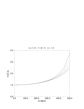
Figure 4: $F(q^{2},0)$ for values of $\alpha$, $\beta$ and $\gamma$ used in Figures 2 and 3.

This figure shows that the variation in the form-factor responsible for the large allowed range of $\hbox{Re}A$ of Figure 3 cannot be seen at all in the region probed by $K_{L}\rightarrow\ell^{+}\ell^{-}\gamma$. This illustrates our claim that a better measurement of $K_{L}\rightarrow\ell^{+}\ell^{-}\gamma$ will not remove the uncertainty in $K_{L}\rightarrow\mu^{+}\mu^{-}$.

Before ending this section we should compare our model calculation to that of Ref. [14]. It may be argued that the model of Ref. [14] has a better physical motivation than the toy models that we use. The authors of Ref. [14] construct their model to incorporate three ingredients: the known low energy behavior of $F(q_{1}^{2},q_{2}^{2})$ (our $\alpha$); the fact that the only poles in the region between the kaon mass and 1 GeV are those generated by the vector meson resonances; and the high $q^{2}$ behavior from perturbative QCD. From these ingredients they reach the conclusion that the uncertainty in $\hbox{Re}A$ is under some control and obtain their bound on $\rho$. Our differences arise because we argue that vector meson dominance for weak decays is nothing more than an assumption. Our toy models allow us to vary the behavior of $F(q_{1}^{2},q_{2}^{2})$ in the region near one GeV, where neither chiral perturbation theory nor perturbative QCD are reliable. We are thus able to show that $\hbox{Re}A$ is quite sensitive to the behavior of the form factor in this matching region, and we argue that this is, in fact, the main source of uncertainty. This is why we conclude that it is impossible at present to estimate $\hbox{Re}A$ reliably. We do not claim to have a physically motivated model for the behavior of $F(q_{1}^{2},q_{2}^{2})$ in the matching region, but simply point out that the conclusion of Ref. [14] follows from their assumption about the behavior of $F(q_{1}^{2},q_{2}^{2})$ in the matching region. We believe that it will not be possible to test that assumption with any precision in the foreseeable future, and, therefore, disagree with their conclusion.

4 Conclusions

We have studied the dispersive contribution of the two-photon intermediate state to the decay $K_{L}\rightarrow\mu^{+}\mu^{-}$. Within chiral perturbation theory we can write the real part of the amplitude in terms of one unknown combination $h(\mu)$. The current experimental measurements of $K_{L}\rightarrow\gamma\gamma$ and $K_{L}\rightarrow\mu^{+}\mu^{-}$ imply that $h(\mu)=8.7\pm 2$. If we cast the short distance amplitude in the same notation, we find that $h_{SD}\sim 3$, of the same order as the uncertainty in the long distance dispersive contribution. We find that there is no process where $h(\mu)$ can be determined separately from $h_{SD}$ and, therefore, conclude that it is impossible to extract information on short distance parameters from the measurement of $K_{L}\rightarrow\mu^{+}\mu^{-}$ within chiral perturbation theory.

We have also found that the rate for $K_{L}\rightarrow e^{+}e^{-}$ is relatively insensitive to the precise value of $h(\mu)$. From this observation we are able to predict $B(K_{L}\rightarrow e^{+}e^{-})\sim 9\times 10^{-12}$.

We have also re-visited the calculation of $\hbox{Re}A$ within models. We have used simple pole models to unitarize the high energy behavior of the off-shell $K\gamma^{*}\gamma^{*}$ vertex as is common in the literature. We have used a class of models that can accommodate the measured low-energy behavior of said vertex while allowing us to vary the form factor in the region near the chiral symmetry breaking scale. From this exercise we find that, the main source of uncertainty in $\hbox{Re}A$ does not arise from the error in the measurement of $\alpha$. In fact, we find that even if the low energy behavior of the $K\gamma^{*}\gamma^{*}$ vertex is precisely measured (in our parameterization this means that $\alpha$ and $\beta$ are well measured), the uncertainty arising from the energy region that is not accessible to experiment is sufficiently large to make $\hbox{Re}A$ impossible to predict.

Our conclusion is, therefore, rather pessimistic. We believe that it will be impossible to extract any information on the short distance parameter $\rho$ from a measurement of $K_{L}\rightarrow\mu^{+}\mu^{-}$ in the foreseeable future. This situation will change only when we are able to calculate reliably the long distance amplitude from QCD.

Acknowledgments

This work was supported in part by the DOE OJI program under contract number DE-FG02-92ER40730. I am grateful to the theory group at SLAC for their hospitality while part of this work was performed. I wish to thank G. Isidori and G. d’Ambrosio for useful discussions and for a critical reading of this manuscript. I also thank J. Donoghue, L. Littenberg and C. Quigg for comments on the manuscript.

References

- [1] M. K. Gaillard and B. W. Lee, Phys. Rev. D10 897 (1974), and correction in M. K. Gaillard, B. W. Lee and R. E. Shrock, Phys. Rev. D13 2674 (1976). An early attempt to extract short distance parameters from this reaction is that of R. E. Shrock and M. B. Voloshin, Phys. Lett. 87B 375 (1979).
- [2] C. Quigg and J. D. Jackson, UCRL-18487 unpublished (1968).
- [3] L. Bergström, E. Massó, P. Singer, Phys. Lett. 131B 229 (1983); L. Bergström, et. al., Phys. Lett. 134B 373 (1984).
- [4] G. Bélanger and C. Q. Geng, Phys. Rev. D43 140 (1991); P. Ko, Phys. Rev. D45 174 (1992); J. O. Eeg, K. Kumericki and I. Picek, hep-ph/9605337.
- [5] J. Ritchie and S. Wojcicki, Rev. of Mod. Phys. 65 1149 (1993).
- [6] L. Littenberg and G. Valencia, Annu. Rev. Nucl. Part. Sci. 43 729 (1993).
- [7] P. Herczeg, Phys. Rev. D27 1512 (1983).
- [8] T. Inami and C. S. Lim, Prog. Theor. Phys. 65 297 (1981).
- [9] A. Buras and R. Fleischer, hep-ph/9704376, to appear in Heavy Flavours II, World Scientific (1997), Eds. A. J. Buras and M. Lindner.
- [10] G. Buchalla, A. Buras and M. Harlander, Nucl. Phys. B349 1 (1991).
- [11] Review of Particle Physics, Particle Data Group, Phys. Rev. D54 (1996).
- [12] A. Heinson, et. al., Phys. Rev. D51 985 (1995).
- [13] T. Akagi, et al., Phys. Rev. Lett. 67 2618 (1991).
- [14] G. d’Ambrosio, G. Isidori and J. Portoles, hep-ph/9708326 (1997).
- [15] K. E. Ohl, et. al., Phys. Rev. Lett. 65 1407 (1990); G. Barr, et. al., Phys. Lett. 240B 283 (1990).
- [16] M. B. Spencer, et. al., Phys. Rev. Lett. 74 3323 (1995).
- [17] J. F. Donoghue, B. R. Holstein and Y. C. Lin, Nucl. Phys. B277 651 (1986).
- [18] See for example, J. F. Donoghue, E. Golowich and B. R. Holstein, Dynamics of the Standard Model Cambridge (1992).
- [19] M. Savage, M. Luke and M. Wise, Phys. Lett. 291B 481 (1992).
- [20] M. Lu, M. Wise and M. Savage, Phys. Rev. D46 5026 (1992).
- [21] M. Savage and M. Wise, Phys. Lett. 250B 151 (1990).
- [22] G. Buchalla and A. Buras, Phys. Lett. 336B 263 (1994).
- [23] G. Ecker, A. Pich and E. de Rafael, Nucl. Phys. B291 692 (1987).
- [24] C. Quigg, private communication.