We investigate the structure of constituent quarks and study implications for quark distribution functions of hadrons. Constituent quarks are constructed by dressing bare quarks with Goldstone bosons using the chiral quark model. We calculate resulting corrections to the twist-2 structure functions $f_{1}(x)$, $g_{1}(x)$ and $h_{1}(x)$. The Goldstone boson fluctuations produce a flavor asymmetry of the quark distribution in the nucleon in agreement with experimental data. They also generate significant depolarization effects which reduce the fraction of the nucleon spin carried by quarks. Corrections to the transversity spin structure function $h_{1}(x)$ differ from those to $g_{1}(x)$, and in particular we find a large reduction ($40\%$) of the $d$-quark tensor charge, which is consistent with recent lattice calculations. We also study the pion structure function and find the momentum fraction carried by the sea quarks in the pion to be considerably larger than that in the nucleon.

PACS numbers: 13.60.Hb, 13.88.+e, 12.39.Fe, 12.39.Ki, 14.40.Aq

Key Words: deep inelastic scattering, nucleon spin structure, constituent quark model, Goldstone boson

1 Introduction

High energy experiments such as lepton-hadron deep inelastic scattering and the Drell-Yan process provide detailed knowledge of the quark and gluon distributions of hadrons. One obtains information about the momentum distribution functions of valence quarks, sea quarks and gluons, and their scaling violations are quite consistent with predictions from perturbative QCD [1]. Even under these circumstances, we still have a most important problem, namely how to understand the structure functions themselves. Perturbative QCD describes their $Q^{2}$ evolution, but cannot predict the distribution functions because of their non-perturbative origin. Although lattice QCD studies provide some moments of the structure functions [2], a satisfactory understanding is still far from being reached.

On the other hand, much of low-energy hadron phenomenology is quite successfully described in terms of the constituent quark picture. At low energies, the sea quark and gluon degrees of freedom are assumed to be absorbed into constituent quarks as quasi-particles, and hadrons are constructed out of a few such quasi-particles. At the high energy scale, sea quarks and gluons reappear and hadrons reveal themselves as complex many-body systems with a large number of current quarks and gluons. We do not yet have a clear understanding of the connection between constituent quarks at low energy and the parton picture at high energy.

Some attempts have been made to model this connection or at least some aspects of it [3, 4, 5, 6]. In such studies, the twist-2 part of a given structure function is evaluated within a relativistic quark model, and the resulting structure function is then evolved from the low-energy scale, where the constituent quark picture is supposed to work, to the high momentum scale with the help of perturbative QCD. Such studies may help to approach the deep inelastic scattering data from the point of view of low-energy non-perturbative dynamics. For example, the observed large deviations of the ratios $F^{n}_{2}(x)/F^{p}_{2}(x)$ and $g_{1}^{p}(x)/F^{p}_{1}(x)$ from the simple parton picture can be understood by taking into account the spin-flavor structure of the nucleon [7, 8] in terms of the structure of constituent quarks. In addition, the difference between the $u$-quark distribution in the pion and the one in the kaon is well reproduced within a chiral model [9] where the constituent quarks play a crucial role.

Despite its successes, the perturbative QCD evolution becomes problematic when it is started from scales far below 1 GeV. In most cases, calculations require that the evolution is performed upward from scales as low as $\mu^{2}\sim 0.1-0.3\mbox{GeV}^{2}$ to reproduce the high $Q^{2}$ experimental data. In this region the use of perturbative QCD may be questionable, even though the difference between results obtained in leading order and next-to-leading order from a scale $\mu^{2}\sim 0.3\mbox{GeV}^{2}$ is only about $10\%$.

Recent studies of Kulagin et al.[5] have shown that such difficulties can be overcome by taking into account the structure of the constituent quarks. It was found that inclusion of the pion dressing and higher mass spectator processes substantially changes the shapes of the quark distributions at the given model scale. This modifies the normalization of the quark distributions and leads to the correct small-$x$ behavior by introducing Regge exchange. The identification of the results in ref. [5] with the twist-2 quark distribution can now be done at a scale of about $1\mbox{GeV}^{2}$, where the use of perturbative QCD for further evolution to high $Q^{2}$ is reasonably justified.

In the present paper we follow a similar direction, although with different emphasis, and extend it to the spin dependent structure functions and to hadrons other than the nucleon. At the scale below 1 GeV, the relevant degrees of freedom are assumed to be constituent quarks (CQ) and Goldstone (GS) bosons[10]. Here, we concentrate on the Goldstone boson dressing in the $SU(3)_{R}\otimes SU(3)_{L}$ chiral quark model with explicit $SU(3)$ flavor symmetry breaking. We study the twist-2 structure functions of the nucleon [11], namely the unpolarized $f_{1}(x)$, the helicity difference $g_{1}(x)$, and the transversity difference $h_{1}(x)$, as well as the pion structure function with inclusion of the CQ structure. While Regge high-energy behaviour was found to be important in previous studies of the unpolarized structure function, primarily at small $x$, our main focus here will be on the “soft” dynamics mediated by the pseudoscalar meson octet. The GS boson cloud influences not only the normalization at the quasi-particle pole of the constituent quarks but also changes their spin structure by emitting the GS bosons into $P$-wave states relative to the CQ, thus producing depolarization effects.

Recently, such a pion dressing has been studied by several authors [12] in order to account for the violation of the Gottfried sum rule and the nucleon spin structure. We first reexamine this previous work systematically. Then we study the chiral-odd transversity spin structure function $h_{1}(x)$. Corrections to $h_{1}(x)$ turn out to differ from those for $g_{1}(x)$. This difference causes a strong reduction of the $d$-quark tensor charge, while the axial charge remains almost unchanged. This tendency seems to be consistent with a recent lattice study [13] which suggests $|\delta d|<|\Delta d|$ as opposed to $\delta u>\Delta u$ for the $u$-quarks.

We also show how the pion structure function modifies with inclusion of CQ structure, in comparison with the nucleon. We find that the resulting sea quark distribution in the pion is substantially enhanced. The contribution to the second moment from the sea quarks in the pion is almost twice as large as that in the nucleon. This issue will possibly be studied in future experiments.

This paper is organized as follows. In Section 2, we construct the constituent quark Fock states and evaluate their contributions to deep inelastic scattering. We examine the Gottfried sum rule and the nucleon spin structure in Section 3, as it was first done by Eichten et al.[12]. In Section 4 we study the chiral-odd transversity spin structure function $h_{1}(x)$ and show that the GS boson dressing of quarks changes the simple quark model result for $h_{1}^{d}(x)$ substantially. Section 5 is focused on the discussion of the pion structure function. We emphasize that the inclusion of the GS boson dressing naturally leads to an enhancement of the sea quarks in the pion. We draw conclusions in the final section with a brief estimate of contributions from multi-pion Fock states.

2 Structure of constituent quarks

We start by constructing the constituent quark Fock state using the chiral quark model of Manohar and Georgi [10]. In this model, constituent quarks couple to the Goldstone bosons of spontaneously broken chiral symmetry. The GS bosons, in particular the pion, play a crucial role as approximate zero modes of the QCD vacuum. They govern the low-energy dynamics at characteristic scales $\mu{{}^{<}_{\sim}}4\pi f_{\pi}\sim 1\mbox{GeV}$ where $f_{\pi}\simeq 93\mbox{MeV}$ is the pion decay constant.

Let $\psi=(u,d,s)$ be the quark field with $N_{f}=3$ flavours. The effective interaction Lagrangian in leading order is given by

$${\cal L}_{\mbox{int}}=-\frac{g_{A}}{f}\bar{\psi}\gamma^{\mu}\gamma^{5}\left(\partial_{\mu}\Pi\right)\psi$$ (1)

with the GS boson matrix field,

$$\Pi={1\over{\sqrt{2}}}\left({\matrix{\frac{\pi^{0}}{\sqrt{2}}+\frac{\eta}{\sqrt{6}}&\pi^{+}&K^{+}\cr\pi^{-}&-\frac{\pi^{0}}{\sqrt{2}}+\frac{\eta}{\sqrt{6}}&{K^{0}}\cr K^{-}&\bar{K}^{0}&-\frac{2\eta}{\sqrt{6}}\cr}}\right)\;\;.$$ (2)

Here, we set the pseudoscalar decay constant $f$ equal to the pion decay constant $f_{\pi}$ and start with the quark axial-vector coupling $g_{A}=1$. In their original work, Manohar and Georgi took $g_{A}=0.75$ to reproduce the nucleon axial-vector coupling constant within the non-relativistic approximation[10]. We first adopt $g_{A}$ = 1 following the large $N_{c}$ argument from ref. [14] and discuss possible renormalization effects later.

The $u$-, $d$- and $s$-quarks that enter in eq. (1) are assumed to have already developed large dynamical masses as a dynamical consequence of spontaneous chiral symmetry breaking. We denote those “bare” but massive states by $\left|u_{0}\right\rangle$ and $\left|d_{0}\right\rangle$ etc. Once they are dressed by GS bosons, we write the constituent $u$- and $d$-quark Fock-states as

$$\left|U\right\rangle = \sqrt{Z}\left|u_{0}\right\rangle+a_{\pi}\left|{d\pi^{+}}\right\rangle+{{a_{\pi}}\over 2}\left|{u\pi^{0}}\right\rangle+a_{K}\left|{sK^{+}}\right\rangle+{{a_{\eta}}\over 6}\left|{u\eta}\right\rangle\,\,,$$ (3-a)

$$\left|D\right\rangle = \sqrt{Z}\left|d_{0}\right\rangle+a_{\pi}\left|{u\pi^{-}}\right\rangle+{{a_{\pi}}\over 2}\left|{d\pi^{0}}\right\rangle+a_{K}\left|{sK^{0}}\right\rangle+{{a_{\eta}}\over 6}\left|{d\eta}\right\rangle\,\,,$$ (3-b)

where $Z$ is the renormalization constant for a “bare” constituent quark and $|a_{i}|^{2}$ are probabilities to find GS bosons in the dressed constituent quark states. The wave function renormalization $Z$ only operates on the bare CQ state, because we use the renormalized quark-meson coupling constants to calculate $a_{i}$. In this paper we restrict our study to the admixture of one GS boson and truncate the Fock space expansion as displayed in eqs. (3-a), (3-b). We shall give an estimate of two-pion Fock state contributions later.

Within this approximation, the diagrams Figs. 1(a) and 1(b) contribute to the structure functions. We use the Infinite Momentum Frame (IMF) to calculate these contributions[15, 16]. By virtue of the IMF, the factorization of the subprocess is automatic and we may neglect possible off-shell corrections, since all the particles are on-mass-shell in this frame. Hence we can use one-dimensional convolution formalism throughout the following calculations. Also, working in the IMF removes the so-called Z-graph contributions.

Figure 1:

Diagrams contributing to the constituent quark structure. Fig.1.(a) shows the GS boson spectator process, whereas Fig.1(b) probes the structure of the GS boson itself, with the constituent quark being spectator. The virtual photon is depicted by the wavy line. Thick sold curves represent the quarks, and the dashed curve the GS boson.

In previous studies we have already obtained the pion dressing corrections to the constituent quark distribution function at a low-momentum scale [5], as follows. The spin-independent term corresponding to diagram 1(a) is given by

$$q_{j}(x)=\int_{x}^{1}{{dy}\over y}\,P_{j\,\alpha/i}(y)\,q_{i}\left({{x\over y}}\right)\;\;.$$ (4)

Here, $P(y)_{j\,\alpha/i}$ is the splitting function which gives the probability to find a constituent quark $j$ carrying the light-cone momentum fraction $y$ together with a spectator GS boson $(\alpha=\pi,K,\eta)$, both of which coming from a parent constituent quark $i$:

$$P(y)_{j\,\alpha/i}={1\over{8\pi^{2}}}\left({{{g_{A}\,\bar{m}}\over{f}}}\right)^{2}\int{dk_{T}^{2}}{{(m_{j}-m_{i}y)^{2}+k_{T}^{2}}\over{y^{2}(1-y)\left[{m_{i}^{2}-M^{2}_{j\alpha}}\right]^{2}}}\;\;,$$ (5)

where $m_{i},m_{j},m_{\alpha}$ are the masses of the $i,j$- constituent quarks and the pseudoscalar meson $\alpha$, respectively. $M^{2}_{j\,\alpha}=\frac{m_{j}^{2}+k_{T}^{2}}{y}+\frac{m_{\alpha}^{2}+k^{2}_{T}}{1-y}$ is the invariant mass squared of the final state, and $\bar{m}$ is the average of the constituent quark masses, $\bar{m}=(m_{i}+m_{j})/2$. The integral (5) requires a cutoff which will be specified later.

Diagram 1(b) probes the internal structure of the GS bosons. This process gives the following contribution:

$$q_{k}(x)=\int{{{dy_{1}}\over y_{1}}}\,{{{dy_{2}}\over y_{2}}}\,V_{k/\alpha}\left(\frac{x}{y_{1}}\right)P_{\alpha\,j/i}\left(\frac{y_{1}}{y_{2}}\right)\,q_{i}(y_{2})\,,$$ (6)

where $P_{\alpha\,j/i}(x)=P_{j\,\alpha/i}(1-x)$. This symmetry relation holds in the IMF if we use a momentum cutoff procedure as in ref. [16]. Here, $V_{k/\alpha}(x)$ is the quark distribution function with flavor $k$ in the GS boson $\alpha$, with the normalization $\int^{1}_{0}{dx}V_{k/\alpha}(x)=1$. When we calculate the quark distribution explicitly in Section 4 and 5, we will use the phenomenological parametrization of the pion structure function at the scale $1\mbox{GeV}^{2}$[18]. As for the kaon and eta, we do not have experimental data and simply use the model calculations of ref. [9, 17]. Ambiguities of the final results arising from the choice of the meson structure functions are rather small, at the level of a few $\%$.

We define the moments of the splitting functions $P_{j\alpha,/i}$,

$$\left\langle x^{n-1}P_{j\,\alpha/i}\right\rangle\equiv\int_{0}^{1}{dx}\;x^{n-1}\;P_{j\,\alpha/i}(x)\;\;.$$ (7)

As for the first moments, $\langle P_{j\,\alpha/i}\rangle=\langle P_{\alpha\,j/i}\rangle\equiv\langle P_{\alpha}\rangle$. In terms of those the renormalization constant $Z$ is then given by

$$Z=1-{3\over 2}\left\langle{P_{\pi}}\right\rangle-\left\langle{P_{K}}\right\rangle-{1\over 6}\left\langle{P_{\eta}}\right\rangle\;\;.$$ (8)

We find $Z\sim 0.7$ using the standard parameter set $g_{A}=1$, $\bar{m}=350$ MeV and a cutoff $\Lambda=4\pi f$ as specified at the end of this Section. Numerically, about 75$\%$ of the deviation from $Z=1$ comes from the pion dressing and 20 $\%$ from the kaons.

As examples, we explicitly write down the quark distribution functions in the nucleon using the splitting functions (5). We assume that the bare quark distribution functions are given in terms of the valence quark distributions $u_{0}(x)$ and $d_{0}(x)$. No antiquarks are present before the GS boson coupling is turned on. We find

$$u(x) = Zu_{0}(x)+P_{u\pi/d}\otimes d_{0}+V_{u/\pi}\otimes P_{\pi\,d/u}\otimes u_{0}+{1\over 2}P_{u\,\pi/u}\otimes u_{0}$$ (9)

$$+{1\over 4}V_{u/\pi}\otimes P_{\pi}\otimes(u_{0}+d_{0})+V_{u/K}\otimes P_{K\,u/u}\otimes u_{0}$$

$$+\frac{1}{6}P_{u\,\eta/u}\otimes u_{0}+{1\over 36}V_{u/\eta}\otimes P_{\eta}\otimes(u_{0}+d_{0})\;\;,$$

$$d(x) = Zd_{0}(x)+P_{\pi}\otimes u_{0}+V_{d/\pi}\otimes P_{\pi}\otimes d_{0}+{1\over 2}P_{\pi}\otimes d_{0}$$ (10)

$$+{1\over 4}V_{d/\pi}\otimes P_{\pi}\otimes(u_{0}+d_{0})+V_{d/K}\otimes P_{K}\otimes d_{0}$$

$$+\frac{1}{6}P_{\eta}\otimes d_{0}+{1\over 36}V_{d/\eta}\otimes P_{\eta}\otimes(u_{0}+d_{0})\;\;,$$

where the bare distribution functions in the proton have the normalizations

$$\int^{1}_{0}{dx}\,u_{0}(x)=2\,,$$

$$\int^{1}_{0}{dx}\,d_{0}(x)=1\,.$$

Here, we use the following short hand notation for the convolution integral:

$$P\otimes q\equiv\int_{x}^{1}{{{dy}\over y}}\,P(y)\,\,q\left({{x\over y}}\right)\;.$$ (11)

For the antiquarks and the strange quarks we find:

$$\bar{u}(x) = V_{u/\pi}\otimes P_{\pi}\otimes d_{0}$$ (12)

$$+\frac{1}{4}V_{u/\pi}\otimes P_{\pi}\otimes(u_{0}+d_{0})+\frac{1}{36}V_{u/\eta}\otimes P_{\eta}\otimes(u_{0}+d_{0})\;,$$

$$\bar{d}(x) = V_{d/\pi}\otimes P_{\pi}\otimes u_{0}$$ (13)

$$+\frac{1}{4}V_{d/\pi}\otimes P_{\pi}\otimes(u_{0}+d_{0})+\frac{1}{36}V_{d/\eta}\otimes P_{\eta}\otimes(u_{0}+d_{0})\;,$$

$$s(x) = P_{K}\otimes(u_{0}+d_{0})+\frac{4}{9}V_{s/\eta}\otimes P_{\eta}\otimes(u_{0}+d_{0})\;,$$ (14)

$$\bar{s}(x) = V_{s/K}\otimes P_{K}\otimes(u_{0}+d_{0})+\frac{4}{9}V_{s/\eta}\otimes P_{\eta}\otimes(u_{0}+d_{0})\;.$$ (15)

We then obtain the valence quark distributions as $u_{val}=u(x)-\bar{u}(x),$ $d_{val}(x)=d(x)-\bar{d}(x)$, which satisfy the correct normalization with the renormalization constant $Z$. For instance, the first moment of the valence $u$-quark is

$$\int^{1}_{0}{dx}u_{val}(x) = \int^{1}_{0}{dx}\left[Zu_{0}(x)+P_{u\pi/d}\otimes d_{0}+V_{u/\pi}\otimes P_{\pi\,d/u}\otimes u_{0}\right.$$

$$\left.+{1\over 2}P_{u\,\pi/u}\otimes u_{0}-V_{u/\pi}\otimes P_{\pi\,u/d}\otimes d_{0}\right.$$

$$\left.+V_{u/K}\otimes P_{K\,u/u}\otimes u_{0}+\frac{1}{6}P_{u\,\eta/u}\otimes u_{0}\right]$$

$$= 2Z+\langle P_{\pi}\rangle+2\langle P_{\pi}\rangle+2\frac{1}{2}\langle P_{\pi}\rangle-\langle P_{\pi}\rangle+2\langle P_{K}\rangle+2\frac{1}{6}\langle P_{\eta}\rangle$$

$$= 2\;\;,$$

where we have used eq. (8) in the last step.

Next we evaluate the spin-dependent process and study the spin distribution of the nucleon. An analogous calculation as the one leading to eq. (5) yields:

$$\Delta P(y)_{j\,\alpha/i}={1\over{8\pi^{2}}}\left({{{g_{A}\bar{m}}\over{f}}}\right)^{2}\int{dk_{T}^{2}}{{(m_{j}-m_{i}y)^{2}-k^{2}_{T}}\over{y^{2}(1-y)\left[{m_{i}^{2}-M^{2}_{j\,\alpha}}\right]^{2}}}\;\;,$$ (16)

where $\Delta P_{j\,\alpha/i}=P_{j\uparrow\,\alpha/i\uparrow}-P_{j\downarrow\,\alpha/i\uparrow}$ is the difference of probabilities to find helicity $+1/2$ quarks minus helicity $-1/2$ quarks starting from a parent quark with helicity $+1/2$. Note the change of sign in front of $k_{T}^{2}$ when comparing $P$ and $\Delta P$. With the standard parameter set mentioned above, this spin dependent splitting function gives a negative contribution, that is, the helicity-flip process is dominant. In previous studies[12], the relation $P=-\Delta P$ has simply been used, assuming that the GS boson emission contributes only to the helicity flip process. However, the ratio of helicity flip and non-flip contributions depends on the dynamics. The magnitude of the spin-dependent splitting function is rather sensitive to the choice of the cutoff, because the helicity-flip probability is directly proportional to the transverse momentum integral. The GS boson dressing given by the formula (16) modifies the axial-vector coupling constant $g_{A}$ of the nucleon as well as the quark content $\Sigma$ of the nucleon spin, as we shall elaborate.

Now we specify the momentum cutoff function at the quark-GS boson vertex. An exponential cutoff is often used in IMF calculations, since such a form factor has the correct $t$ and $u$ channel symmetry[16]:

$$g_{A}\rightarrow g_{A}\;\,\mbox{exp}\left[\frac{m_{i}^{2}-M^{2}_{j\,\alpha}}{4\Lambda^{2}}\right]\;.$$ (17)

Here $\Lambda$ is the cutoff parameter. This function satisfies the proper symmetry, $P_{j\alpha/i}(y)=P_{\alpha j/i}(1-y)$. The value of the cutoff is taken to be about $\Lambda\sim 4\pi f_{\pi}\sim 1\mbox{GeV}$, the characteristic scale of spontaneous chiral symmetry breaking. In actual calculations it will be determined to reproduce the experimental data of the Gottfried sum rule.

Using this cutoff function, we show in Fig.2 the constituent quark-Goldstone boson splitting functions, $P_{j\alpha/i}(y)$ and $\Delta P_{j\alpha/i}(y)$, for the case of a $u$-quark $(i=j=u)$ together with the pion $(\alpha=\pi)$ and $\Lambda=1.4\mbox{GeV}$. For the constituent quark masses, we use $m_{u}=m_{d}=360\mbox{MeV}$ and $m_{s}=570\mbox{MeV}$ as typical values guided by NJL model calculations[24] and phenomenology. The resulting splitting function $P_{u\alpha/u}$ is peaked at $y<0.4$, and $\Delta P_{j\alpha/i}$ is negative over most of the $y$ range. If we choose smaller values for the cutoff $\Lambda$ (say, $\Lambda=0.5\mbox{GeV}$), $\Delta P_{j\alpha/i}$ becomes positive but stays very small.

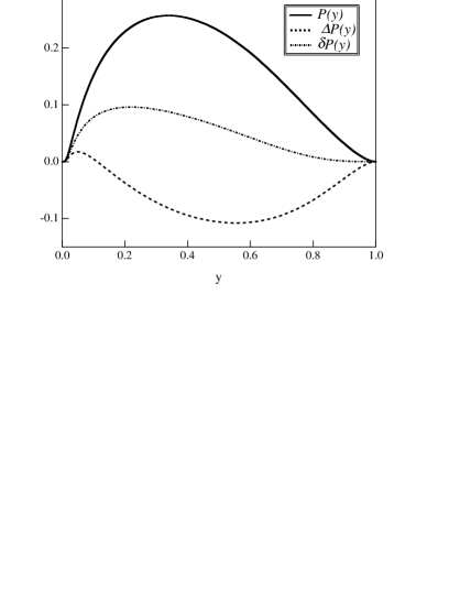
Figure 2:

Constituent quark-GS boson splitting functions for twist-2 structure functions. $P_{j{\pi}/i}(x)$, $\Delta P_{j{\pi}/i}(x)$ and $\delta P_{j{\pi}/i}(x)$ are shown by the solid, dashed and dash-dotted curves, respectively.

3 Gottfried sum and nucleon spin in the chiral quark model
3.1 Update of the Gottfried sum rule

We start this Section by re-examining the effects of the GS boson fluctuations on the Gottfried sum rule and the nucleon spin structure. These were first discussed by Eichten et al.[12]. The Gottfried sum rule (GSR) is given in terms of the difference of the proton and neutron structure functions:

$$GSR=\int_{0}^{1}{\frac{dx}{x}\;}\left[{F_{2}^{p}(x)-F_{2}^{n}(x)}\right]={1\over 3}\int^{1}_{0}{dx}\left({u(x)+\bar{u}(x)-d(x)-\bar{d}(x)}\right)\;.$$ (18)

A naive parton model with isospin symmetric sea, $\bar{u}=\bar{d}$, yields $GSR$ = 1/3, whereas the experimentally observed value is $0.235\pm 0.026$[19], which indicates isospin symmetry breaking $\bar{u}(x)<\bar{d}(x)$ in the nucleon sea. If we take into account the shadowing correction to extract the neutron structure function from the deuteron data, the GSR value is further reduced by about 20-30$\%$ [20]. With this correction, the empirical value of the GSR is reduced to about $0.21-0.22$.

We now employ the quark distribution functions of the chiral quark model as given in Section 2. Inserting the expressions (9,10,12,13) into eq. (18), one gets

$$GSR = {1\over 3}\left({Z-{1\over 2}\left\langle{P_{\pi}}\right\rangle+\left\langle{P_{K}}\right\rangle+{1\over 6}\left\langle{P_{\eta}}\right\rangle}\right)$$ (19)

$$= {1\over 3}\left(1-2\left\langle{P_{\pi}}\right\rangle\right)\;.$$

With the parameters discussed in Section 2, the renormalization constant is found to be $Z\sim 0.7$. Here, we adopt $\Lambda=1.4\mbox{GeV}$ for the cutoff function eq. (17), and obtain $Z=0.67$, $\left\langle{P_{\pi}}\right\rangle=0.16$, $\left\langle{P_{K}}\right\rangle=0.09$ and $\left\langle{P_{\eta}}\right\rangle=0.06$. We then find 0.22 for $GSR$, in good agreement with the empirical value. The dominant contribution to the reduction of GSR comes from the renormalization of the bare quark state represented by the $Z$ factor. The value $\Lambda=1.4\mbox{GeV}$ should be understood as an upper bound of the cutoff in the chiral quark model, based on the assumption that the violation of the Gottfried sum is entirely given by the Goldstone boson dressing alone. One should note, of course, that this $\Lambda$ depends on the input constituent quark mass. If we choose $\bar{m}\simeq 400\mbox{MeV}$, the resulting cutoff turns out to be about $\Lambda\simeq 1.1\mbox{GeV}$.

3.2 Angular momentum transfer to the meson cloud

Next we discuss the spin structure of the nucleon. Analysis of all available experimental data[21] gives the following decomposition of the nucleon spin in terms of the quark spin, with $\Delta q=q\uparrow-q\downarrow+\bar{q}\uparrow-\bar{q}\downarrow$:

$$\Delta u=0.82\pm 0.02,\hskip 28.45274pt\Delta d=-0.43\pm 0.02,\hskip 28.45274pt\Delta s=-0.10\pm 0.02,$$

$$\Sigma\equiv\Delta u+\Delta d+\Delta s=0.29\pm 0.06$$ (20)

at $Q^{2}=5\mbox{GeV}^{2}$, to be compared with expectations of the naive quark models ($\Sigma=1$) or with inclusion of relativistic corrections $(\Sigma\sim 2/3)$. Using the spin-dependent splitting functions (16), the spin fractions of the constituent quarks are modified from their bare quark values as follows:

$$\Delta u=Z\Delta u_{0}+\frac{1}{2}\left\langle{\Delta P_{\pi}}\right\rangle\Delta u_{0}+\left\langle{\Delta P_{\pi}}\right\rangle\Delta d_{0}+\frac{1}{6}\left\langle{\Delta P_{\eta}}\right\rangle\Delta u_{0}\;,$$ (21)

$$\Delta d=Z\Delta d_{0}+\frac{1}{2}\left\langle{\Delta P_{\pi}}\right\rangle\Delta d_{0}+\left\langle{\Delta P_{\pi}}\right\rangle\Delta u_{0}+\frac{1}{6}\left\langle{\Delta P_{\eta}}\right\rangle\Delta d_{0}\;,$$ (22)

$$\Delta s=\left\langle{\Delta P_{K}}\right\rangle(\Delta u_{0}+\Delta d_{0})\;,$$ (23)

where we have assumed $\Delta s_{0}=0$ at the moment. Recall that the first moments $\langle\Delta P\rangle$ of the spin-dependent splitting functions $\left\langle{\Delta P_{\pi}}\right\rangle$ are negative, i.e. the spin-flip probability is larger than the spin non-flip one in the pion emission process. We find $\left\langle{\Delta P_{\pi}}\right\rangle=-0.06$, $\left\langle{\Delta P_{K}}\right\rangle=-0.01$, and $\left\langle{\Delta P_{\eta}}\right\rangle=-0.03$. The pion emission process converts part of the spin of the constituent quark into (P-wave) angular momentum of the meson cloud.

In order to obtain numerical results, initial input spin fractions $\Delta u_{0}$ and $\Delta d_{0}$ are needed. As a first rough estimate, we start from the naive $SU(6)$ quark model values, $\Delta u_{0}={\frac{4}{3}}$, $\Delta d_{0}=-\frac{1}{3}$, which yield the nucleon axial-vector coupling constant $G_{A}=\Delta u_{0}-\Delta d_{0}=5/3$ and the nucleon spin $\Sigma=\Delta u_{0}+\Delta d_{0}=1$ in the absence of the GS boson dressing. Inserting these values into eqs. (21,22,23), we obtain

$$\Delta u=0.86,\hskip 28.45274pt\Delta d=-0.29,\hskip 28.45274pt\Delta s=-0.006.$$

With inclusion of the GS boson dressing the nucleon axial-vector coupling constant becomes

$$G_{A}\equiv\Delta u-\Delta d=1.15\;,$$ (24)

in reasonable agreement with the empirical value. The total quark fraction of the nucleon spin is then given by

$$\Sigma\equiv\Delta u+\Delta d+\Delta s=0.56$$ (25)

This value is about twice as large as the empirical $\Sigma=0.29\pm 0.06$ [21]. If we allow ourselves to vary the momentum space cutoff, it would be possible to obtain a value around $\Sigma\sim 0.3$. However, the agreement with the nucleon axial-vector coupling constant $G_{A}$ is then lost. We therefore conclude that the nucleon spin problem cannot be solved by the GS boson dressing alone, but the depolarization caused by the P-wave coupling to the GS bosons is nevertheless a significant effect.

The value of $\Sigma$, eq.(25), indicates that about 40$\%$ of the nucleon spin is carried by the relative orbital angular momentum between constituent quarks and their pseudoscalar meson clouds. This result is quite consistent with the recent analysis of the nucleon spin decomposition, according to which about $\sim 30\%$ of the nucleon spin is carried by the quark orbital angular momentum [22]. This apparent agreement is of some interest.

3.3 Axial anomaly effects

Let us now investigate some necessary further steps. In the present framework, we deal only with the $SU(3)$ octet of Goldstone bosons to build up the constituent quark structure; we do not incorporate the contribution of the axial $U(1)$ anomaly to the nucleon spin. After the EMC, SMC and SLAC measurements, many efforts have been made to connect the missing nucleon spin with the $U(1)_{A}$ anomaly of QCD. Such anomaly contributions to the spin structure of the constituent quarks have been estimated [23] using the three flavour Nambu and Jona-Lasinio model which dynamically produces spontaneous chiral symmetry breaking and incorporates the axial $U(1)$ anomaly in the form of ’t Hooft’s effective interaction between quarks [24]. Mean field effects from such interactions induce a non-trivial spin structure of constituent quarks such that the spin fractions change from their “bare” values $\Delta u_{0}=4/3$, $\Delta d_{0}=-1/3$ and $\Delta s_{0}=0$ already before GS boson fluctuations are turned on. In a scenario with maximal $\eta$-$\eta^{\prime}$ mixing and with inclusion of relativistic bound state wave functions, Yabu et al. find [23],

$$\Delta u_{0}=0.91,\hskip 28.45274pt\Delta d_{0}=-0.37,\hskip 28.45274pt\Delta s_{0}=-0.12\;\;.$$ (26)

This result shows the screening of the singlet axial charge induced by the quark-antiquark polarization. The dressing with pseudoscalar mesons should be viewed as an additional effect beyond the mean field level. It is therefore meaningful not to start from the standard $SU(6)$ symmetric relation, but to adopt the values quoted in (26). In this case the strange quarks are primordially polarized, and thus the formula obtained previously is slightly modified. We then find a smaller and reasonable value for the nucleon spin as expected.

$$\Sigma=0.20,$$

$$\Delta u=0.60,\hskip 28.45274pt\Delta d=-0.28,\hskip 28.45274pt\Delta s=-0.12\;.$$ (27)

However, although the total spin sum $\Sigma$ is now consistent with the empirical value $0.29\pm 0.06$[21], the individual spin fractions of $u$- and $d$ quarks disagree with the data, and hence the resulting nucleon axial-vector coupling constant $G_{A}=0.85$ is about $30\%$ smaller than the empirical one.

3.4 Pion contribution to the axial-vector coupling constant

At this point, we should emphasize that the pion cloud also contributes directly to the axial-vector matrix elements illustrated schematically in Fig.3(b), in addition to the contributions already discussed above (Fig.3(a)) which are nothing but the renormalization and depolarization effects due to GS boson emission. In fact, within chiral models of the nucleon such as the chiral bag model, the contribution from the pion cloud can be explicitly calculated[25]. In the chiral limit, $m_{\pi}=0$, the pseudoscalar current induced by the pion contributes to the axial-vector matrix element due to the zero mass pion pole. One can show [26] that the magnitude of the pion cloud contribution Fig.3(b) is half of the quark one, Fig.3(a). The nucleon axial-vector coupling constant eq. (24) is then modified as

$$G_{A}\,s_{\mu} = \langle P|\bar{\psi}\gamma_{\mu}\gamma_{5}{\tau_{3}}\psi|P\rangle$$

$$= (\Delta u-\Delta d)s_{\mu}$$

$$= [(\Delta u_{a}+\Delta u_{b})-(\Delta d_{a}+\Delta d_{b})]s_{\mu}$$

$$\sim 1.5(\Delta u_{a}-\Delta d_{a})\,s_{\mu}\;,$$

where $\Delta q_{a}$ are the contributions from diagram 3(a), essentially the same as those calculated in the previous subsection, and $\Delta q_{b}$ comes from the pion pole, Fig.3(b). Note that this pion effect contributes selectively only to the isovector axial-vector matrix elements $G_{A}^{(3)}\equiv G_{A}$. It does not change the flavor singlet axial current and therefore leaves the spin $\Sigma=G_{A}^{(0)}$ untouched, $\Delta u_{b}+\Delta d_{b}=0$. Hence this additional effect may well increase $G_{A}$ to compensate for the small value obtained in eq. (27), with the total spin being unchanged. Indeed, we can obtain the following results including the pion contribution of Fig.3(b) in the chiral limit:

$$\Delta u=0.93,\hskip 28.45274pt\Delta d=-0.43,\hskip 28.45274pt\Delta s=-0.12,$$

$$G_{A}=1.35,$$

$$\Sigma=0.21\;,$$

where we have used eq. (26) as input for the bare spin distribution and introduce the cutoff such as to reproduce the GSR. The resulting spin fractions are now reasonably consistent with the empirical ones, eq. (20), although the axial-vector coupling is somewhat overestimated in the chiral limit, $m_{\pi}\rightarrow 0$.

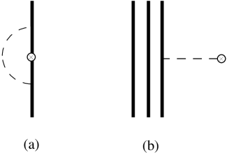
Figure 3:

Contributions to the axial-vector matrix element from the pion cloud. Notations are the same as those in Fig.1, and the circle denotes the insertion of the axial-vector current. The diagram (a) is basically the same as Fig.1(a). The diagram (b) is the pion cloud effect discussed in the text.

In the case of the physical pion with $m_{\pi}\sim 140\mbox{MeV}$, we do not have the soft pion pole, but the axial-vector current itself is changed as

$$A^{a}_{\mu}=\bar{\psi}\gamma_{\mu}\gamma_{5}\frac{\tau^{a}}{2}\psi+f_{\pi}\partial_{\mu}\pi^{a}\;.$$ (28)

We must rely on some specific model to calculate the second term of eq. (28), which is beyond the purpose of this paper. The results are model dependent[27], and as a consequence we cannot draw strong conclusions about the detailed role of such additional pion effects. The tendency of the pion cloud to selectively increase the (isovector) axial constant $G_{A}$ is nevertheless obvious. As a sideremark we note that it is also interesting to study the Bjorken-$x$ dependence of the quark distribution function arising from such pion components, which is expected to be centered in the small-$x$ region.

3.5 Cutoff dependence

One might argue that introducing a cutoff as in eq. (17) implies a high degree of arbitrariness. On the other hand, a distinction between “soft” and “hard” scales is needed, the soft physics being represented by the chiral effective lagrangian. Short distance dynamics, not incorporated in the leading order effective interaction (1), must then reappear in finite size effects parameterized by form factors with a cutoff related to the chiral symmetry breaking scale. For completeness we have investigated other forms of the momentum cutoff function in order to estimate uncertainties inherent in the cutoff procedure. Consider first a sharp cutoff for the transverse momentum, $\theta(\Lambda^{2}-k_{T}^{2})$. To reproduce the observed value of the Gottfried sum the cutoff is the found to be $\Lambda=0.6\mbox{GeV}$. In this case the resulting renormalization factor of the constituent quark wave function is $Z=0.63$, and the first moments of the splitting functions are given by $\langle P_{\pi}\rangle=0.17$ and $\langle\Delta P_{\pi}\rangle=-0.04$. Note that the magnitude of $\langle\Delta P_{\pi}\rangle$ is smaller than the one obtained with a Gaussian cutoff, that is, the depolarization effect by coupling to the pion becomes smaller. When we adopt the input spin fractions of Yabu et al., eq. (26), we find $\Delta u=0.57$, $\Delta d=-0.25$, $\Delta s=-0.11$ and $\Sigma=0.20$, not far from the values, eqs. (27).

We have also used a dipole form for the cutoff, $\left(\frac{\Lambda^{2}+m_{i}^{2}}{\Lambda^{2}+M_{j\alpha}^{2}}\right)^{2}$. Here we need $\Lambda=2.4\mbox{GeV}$ to account for the GSR. The resulting renormalization factor is $Z=0.65$. The calculated spin fractions carried by quarks are $\Delta u=0.58$, $\Delta d=-0.28$, $\Delta s=-0.12$ and $\Sigma=0.18$. As a common feature of all those different cutoff procedures, we note that the leading effect on the $\Delta q$’s still comes from wave function renormalization represented by the $Z$-factor (8). We obtain similar values for this $Z$-factor in all cases, once the cutoff is fixed to reproduce the GSR. From these studies we learn that the cutoff scheme dependence of the results is within $10\%$.

3.6 Discussion

The limitations of the GS boson dressing model to explain the nucleon spin structure are obvious. First, no antiquark polarization is produced in this approach, because the antiquarks are locked into the GS bosons which carry no spin. However, experimental data indicate that the antiquark polarization is not negligible. Several lattice calculations also show that the so-called disconnected parts, which may involve the effects of the $U(1)_{A}$ anomaly and OZI-violating processes, give substantial and negative contributions to the quark polarization[2]. Such contributions are not incorporated in the diagrams of Fig.1(a) and (b).

Another restriction is the smallness of the strange quark polarization. In the original work by Eichten et al., a large strange quark polarization was obtained[12]. However, once the $SU(3)$ flavor symmetry breaking is taken into account, the strange quark polarization from the GS boson couplings turns out to be small. We recall that the numerator of the spin-dependent splitting function is given by $(m_{1}x-m_{2})^{2}-k_{T}^{2}$. For $u,d$ quarks with $m_{1}=m_{2}=m_{u}$, the typical scale of the transverse momentum $k_{T}$ is larger than the constituent quark mass, and thus the splitting function becomes negative. On the other hand, in the strange quark production process, we have $m_{1}=m_{u}$ and $m_{2}=m_{s}$. The large strange quark mass cancels the negative contribution from the transverse momentum integral. Therefore, the spin-dependent splitting function for the strange quark production becomes quite small.

Of course, GS boson dressing is not the only mechanism in question. We have pointed out that it should be seen in combination with other screening effects, involving e.g. the axial anomaly and OZI-violating processes, which renormalize the spin structure of constituent quarks as in eq. (26). The sum of all effects has some analogy with the Arima-Horie renormalization of nucleon $g$-factors in nuclei[28].

It is nevertheless interesting that the GS bosons carry about $35\%$ of the total nucleon spin. Recently, Ji has discussed a gauge invariant decomposition of the nucleon spin [22]. It is suggested that the nucleon spin is carried in parts by the quark spin ($\sim 20\%$), the quark (and antiquark) angular momentum ($\sim 30\%$), and the gluons $(\sim 50\%$) at the low energy scale[22]. Such a scenario will possibly be tested in future experiments, e.g. by deeply virtual Compton scattering off nucleons.

4 Corrections to the chiral-odd structure function $h_{1}(x)$

We have already discussed the spin-independent quark distribution function $f_{1}(x)$ and spin-dependent one $g_{1}(x)$ in the previous sections. We now focus on the chiral-odd transversity structure function $h_{1}(x)$[11]. The longitudinally polarized structure function $g_{1}(x)$, which is chiral-even and can thus be observed in deep inelastic scattering, gives the helicity difference of quarks and antiquarks in the longitudinally polarized nucleon. On the other hand, the chiral-odd $h_{1}(x)$ structure function corresponds to a target helicity-flip amplitude in the standard helicity basis, and thus does not have a simple partonic probability interpretation. The $h_{1}(x)$ structure function provides a correlation between the left- and right-handed quarks due to its chiral-odd nature. Although $h_{1}(x)$ is not identified with quark spin fraction of the nucleon, the transversity structure function $h_{1}(x)$ can be understood as the difference of the numbers of quarks with eigenvalues $+1$ and $-1$ of the transverse Pauli-Lubanski operator $S_{T}\gamma_{5}$ in the transversely polarized nucleon[11]. Unlike the axial charge of the $g_{1}(x)$ distributions, the gluon operators which contribute to $h_{1}(x)$ do not mix quark operators under renormalization because of the chirality. The analysis of $h_{1}(x)$ therefore gives complementary information on the nucleon spin structure.

Naive non-relativistic quark models predict $f_{1}(x)=g_{1}(x)=h_{1}(x)$. Relativistic quark models such as the MIT bag model give a relation $|h_{1}(x)|\geq|g_{1}(x)|$ due to the role of the lower components of the quark Dirac wave function[11]. In such models, the following simple expressions are obtained for the first moments of $g_{1}(x)$ and $h_{1}(x)$, the axial charge $\Delta q$ and tensor charge $\delta q$:

$$|\Delta q| \sim \int d^{3}r[F^{2}-\frac{1}{3}G^{2}]\;,$$

$$|\delta q| \sim \int d^{3}r[F^{2}+\frac{1}{3}G^{2}]\;,$$

where $F$ and $G$ are the upper and lower components of the quark Dirac spinor. Recent lattice simulations indicate that the tensor charge is larger than the axial charge for the $u$-quark, whereas the magnitude of the tensor charge becomes smaller than the axial one for the $d$-quark [13], results which disagree with simple bag model expectations. Here, we study how the pion dressing modifies the $h_{1}(x)$ spin structure function.

Since the $h_{1}(x)$ structure function is chiral-odd, it cannot be measured by a chiral-even probe such as the electro-magnetic interaction. Following the work of Ioffe and Khodjiamirian[29], we introduce the chiral-odd forward scattering amplitude

$$T_{\mu}(q,p,s)=\frac{i}{2}\int{d^{4}\xi e^{iq\cdot\xi}\left\langle{p,S|T\{J_{\mu 5}(\xi)\,J(0)+J(\xi)\,J_{\mu 5}(0)\}|p,S}\right\rangle}\;,$$ (29)

where $J_{\mu 5}=\bar{\psi}\gamma_{\mu}\gamma^{5}\psi$ is the axial-vector current and $J=\bar{\psi}\psi$ the scalar current. This amplitude is related with the chiral-odd structure function $h_{1}(x)$ through the optical theorem. One can write

$$T_{\mu}(q,p,s)=\left({s_{\mu}-{{p\cdot q}\over{q^{2}}}q_{\mu}}\right)\tilde{h}_{1}(x)+\cdots$$ (30)

and obtains the transversity spin distribution function as

$$h_{1}(x)=-\frac{1}{\pi}\mbox{Im}\tilde{h}_{1}(x)$$ (31)

We use the same techniques as in Section 2 to evaluate the GS boson correction to $h_{1}(x)$. The splitting function for the transversity difference is given by,

$$\delta P(y)_{j\,\alpha/i}={1\over{8\pi^{2}}}\left({{{g_{A}\bar{m}}\over{f_{\pi}}}}\right)^{2}\int{dk_{T}^{2}}{{(m_{j}-m_{i}y)^{2}}\over{y^{2}(1-y)\left[{m_{i}^{2}-M^{2}_{j\,\alpha}}\right]^{2}}}$$ (32)

This result tells us that a relation

$$P(x)+\Delta P(x)=2\delta P(x)$$ (33)

holds among the GS boson corrections, which implies a saturation of Soffer’s inequality [30] in the chiral quark model. The calculated splitting function $\delta P_{j\,\alpha/i}$ is shown in Fig.2 together with $P_{j\,\alpha/i}$ and $\Delta P_{j\,\alpha/i}$. Note that $\delta P(x)$ is small and positive in the whole $x$ region, in contrast to the negative longitudinal splitting function $\Delta P(x)$. The first moment of the transversity splitting function is

$$\left\langle{\delta P_{\pi}}\right\rangle=0.05\;,$$

to be compared with $\left\langle{P_{\pi}}\right\rangle=0.16$ and $\left\langle{\Delta P_{\pi}}\right\rangle=-0.06$. The sign difference between $\delta P$ and $\Delta P$ causes a non-negligible modification for the $d$-quark distribution functions. Since the numerator of the transversity splitting function is independent of the transverse momentum, $\langle\delta P\rangle$ is insensitive to the choice of the momentum cutoff.

In order to estimate the GS boson corrections explicitly, we need the bare quark distributions as inputs. Here and for convenience, we use a covariant quark-diquark model, which has already been studied in the literature[8, 31, 32] to obtain the input distributions for $f_{1}(x)$, $g_{1}(x)$ and $h_{1}(x)$.

Assuming $SU(4)$ spin-flavor symmetry, quark distribution functions of bare constituent quarks can be written as

$$u_{0}(x) = 2S_{f}(x),\hskip 28.45274ptd_{0}(x)=S_{f}(x),$$

$$\Delta u_{0}(x) = \frac{4}{3}S_{g}(x),\hskip 28.45274pt\Delta d_{0}(x)=-\frac{1}{3}S_{g}(x),$$

$$\delta u_{0}(x) = \frac{4}{3}S_{h}(x),\hskip 28.45274pt\delta d_{0}(x)=-\frac{1}{3}S_{h}(x).$$

Expressions for $S_{f}(x),S_{g}(x),S_{h}(x)$ are given explicitly in refs. [8, 31, 32]. The relation $S_{h}(x)>S_{g}(x)$ is satisfied as in the bag model calculation[11]. We do not have to elaborate the input distributions here, since the essential features of the following results are independent of the shape of these functions.

As a consequence of the GS boson dressing, the spin-dependent distribution functions for $u$-and $d$-quarks are modified in the following way:

$$\Delta u(x) = Z\Delta u_{0}(x)+\frac{1}{2}\Delta P_{\pi}\otimes\Delta u_{0}+\Delta P_{\pi}\otimes\Delta d_{0}+\frac{1}{6}\Delta P_{\eta}\otimes\Delta u_{0}$$ (34)

$$= \frac{4}{3}ZS_{g}+\frac{1}{3}\Delta P_{\pi}\otimes S_{g}+\frac{2}{9}\Delta P_{\eta}\otimes S_{g}\;,$$

$$\delta u(x) = \frac{4}{3}ZS_{h}+\frac{1}{3}\delta P_{\pi}\otimes S_{h}+\frac{2}{9}\delta P_{\eta}\otimes S_{h}\;,$$ (35)

$$\Delta d(x) = Z\Delta d_{0}(x)+\frac{1}{2}\Delta P_{\pi}\otimes\Delta d_{0}+\Delta P_{\pi}\otimes\Delta u_{0}+\frac{1}{6}\Delta P_{\eta}\otimes\Delta d_{0}\;,$$ (36)

$$= -\frac{1}{3}ZS_{g}+\frac{7}{6}\Delta P_{\pi}\otimes S_{g}-\frac{1}{18}\Delta P_{\eta}\otimes S_{g}\;,$$

$$\delta d(x) = -\frac{1}{3}ZS_{h}+\frac{7}{6}\delta P_{\pi}\otimes S_{h}-\frac{1}{18}\delta P_{\eta}\otimes S_{h}$$ (37)

We show in Figs.4 the spin-dependent $u$-quark distributions in the proton, $\Delta u(x)$ and $\delta u(x)$, together with the unpolarized distribution $u(x)$. Results with inclusion of GS boson fluctuations are given by the solid curves, the ones without the GS bosons by the dashed lines. The renormalization of the constituent quark wave function reduces these distribution functions from their original distributions, and the small-$x$ region is enhanced by the GS bosons. However, the relative magnitudes of $u(x)$, $\Delta u(x)$ and $\delta u(x)$ are not modified very much. The first moments of $\Delta u(x)$ and $\delta u(x)$ are shown in Table 1 with corresponding moments of the original distribution functions.

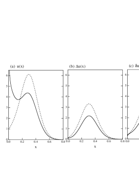
Figure 4:

The $u$-quark distribution functions: (a) $u(x)$, (b) $\Delta u(x)$ and (c) $\delta u(x)$, respectively. In each figure, the result with dressed constituent quarks is shown by the solid curve, the one without the dressing by the dashed curve. Here we use the following parameters to obtain the input bare distributions (dashed): quark mass 0.36GeV, diquark mass 0.7GeV and a cutoff 0.8GeV in the quark-scalar diquark model[32]. Contributions from the pion tail Fig.3(b) to the axial charge are not included.

Effects of the GS boson dressing are more apparent in the $d$-quark case shown in Figs.5. The original distributions satisfy $|\delta d_{0}(x)|\geq|\Delta d_{0}(x)|$. Once the dressing corrections are turned on, $|\delta d_{0}(x)|$ becomes considerably smaller. In the $\Delta d(x)$ distribution function, the corrections from the renormalization and $\langle\Delta P\rangle$ cancel each other, and the resulting $\Delta d(x)$ is not much modified. On the other hand, both contributions are positive for $\delta d(x)$, and hence the transversity of the $d$-quarks is reduced drastically.

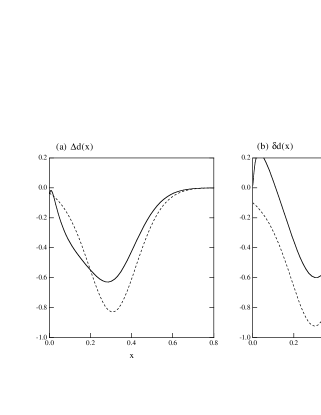
Figure 5:

The $d$-quark distribution functions: (a) $\Delta d(x)$ and (b) $\delta d(x)$, respectively. Notations are the same as those of Fig.4.

The first moments are tabulated in Table 1. The original quark-diquark model without the CQ internal structure predicts the universal inequality $|\Delta q|<|\delta q|$. The GS boson dressing then changes the moments of the $d$-quark, and $|\Delta d|>|\delta d|$ is obtained. We find that the $d$-quark tensor charge is reduced by about $40\sim 50\%$. This result is essentially parameter independent and applies for any model calculation. We note that the smallness of the $d$-quark tensor charge is also obtained within the QCD sum rule approach. In recent work He and Ji find $\delta u=1.33\pm 0.55$ and $\delta d=0.04\pm 0.02$ [33].

Table 1

	$\Delta u$	$\Delta d$	$\delta u$	$\delta d$
Bare	1.01	$-0.25$	1.17	$-0.29$
With CQ	0.65	$-0.22$	0.80	$-0.15$
Exp.	$0.82\pm 0.02$	$-0.43\pm 0.02$	$-$	$-$
Lattice	0.76	$-0.35$	0.84	$-0.23$

The first moments of the helicity and transversity distribution functions. Results with bare quarks and dressed quarks are shown in the second and third columns, respectively. Experimental data[21] and the lattice simulations[13] are also shown in the fourth and fifth columns. Here we use the following parameters: quark mass 0.36GeV, diquark mass 0.7GeV and a cutoff 0.8GeV in the quark-scalar diquark model[32]. Contributions from the pion tail Fig.3(b) to the axial charge are not included.

It is worthwhile mentioning here that the disconnected contribution in the lattice QCD simulation to $h_{1}(x)$ is negligibly small. This situation is quite different from the helicity distribution $g_{1}(x)$, for which the disconnected parts are sizeable.

We comment on recent developments in the perturbative evolution of the $h_{1}(x)$ structure function[34]. The Altarelli-Parisi splitting kernel for $h_{1}(x)$ is different from the standard one for the spin structure function. Barone et al.[35] found that, even if $h_{1}(x)$ and $g_{1}(x)$ are similar at a low starting scale $\sim 0.5\mbox{GeV}$ as suggested by simple quark models, $h_{1}(x)$ becomes much smaller than $g_{1}(x)$ for small $x<0.1$ at the experimentally accessible scale due to the difference in the $Q^{2}$ evolution. On the other hand, the GS boson cloud effects studied in the present paper show up at intermediate values of the Bjorken variable, $0.1<x<0.5$. In particular the $d$-quark contribution to $h_{1}(x)$ is much reduced around $x=0.2\sim 0.3$ from the simple quark model estimate. The GS boson effect also reduces the $d$-quark tensor charge very much as already pointed out. We conclude that the GS boson cloud effects, if existent, should be seen experimentally in the intermediate $x$ region.

In this paper we omit the Regge-type contributions at small-$x$, although significant effects for the unpolarized structure function were found in ref. [5]. It is clearly an interesting point, still under investigation, to combine the GS boson cloud effects presented here and Regge phenomenology in order to reach a unified picture of non-perturbative features at all $x$. Small-$x$ behaviour was studied for $g_{1}(x)$[36] and $h_{1}(x)$[37] within the leading logarithmic approximation of perturbative QCD, and interesting differences were found.

5 Sea quark distributions in the pion and the nucleon

In the framework of the chiral quark model, constituent quarks and Goldstone bosons are treated as quasi-particles. They appear structure-less at the tree-level. As shown in previous sections, however, the dressing of quarks plays an important role in understanding the nucleon structure. Here we try to describe the pion in the similar way, and see how the pion structure function changes when including higher order corrections derived from the effective Lagrangian of the chiral quark model. We specially concentrate on the sea quarks in the nucleon and the pion and show that the sea quark momentum fraction in the pion is expected to be significantly larger than that of the nucleon.

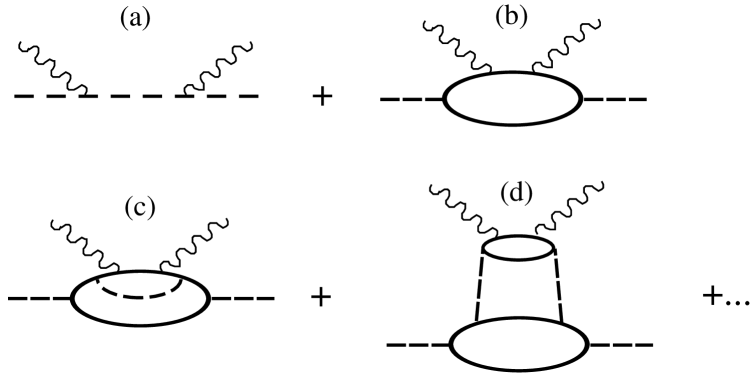
Figure 6:

Typical diagrams contributing to the substructure of the pion in the chiral quark model

Typical diagrams contributing to the pion-virtual photon forward scattering amplitude are displayed in Fig.6. The first diagram, Fig.6(a), represents the elementary pion process (i.e. elastic Compton scattering on the pion) and does not contribute to the leading twist distribution. The second graph, Fig.6(b), can be calculated within the CQM as a first non-trivial contribution. We denote this distribution function by $V_{q/\pi}(x)$ and associate it with the valence quark and antiquark content of the pion. The third and forth diagrams, Fig.6(c)-(d), correspond to the case in which the quark or the antiquark in the second diagram is dressed by the Goldstone bosons. These contributions can be evaluated by using the procedure developed in the Section 2. Such processes determine the sea quark distribution of the pion in the chiral quark model.

We have already given expressions for the quark distribution of the nucleon in eqs. (9,10,12,13). The sea quark distribution in the nucleon is

$$S_{N}(x)=2\bar{u}(x)+2\bar{d}(x)+s(x)+\bar{s}(x)\;.$$ (38)

Such sea quark distribution functions arise from the diagram, Fig.1(b), in which the constituent quarks act as spectators. The contribution from this diagram is soft and concentrated in the small $x$ region as a result of the double convolution.

On the other hand, for the $\pi^{+}$ case in which $u_{0}$ and $\bar{d}_{0}$ are bare quark distributions, the non-valence components that arise from the dressing are given by

$$\bar{u}(x) = P_{\pi}\otimes\bar{d}_{0}+{1\over 4}V_{u/\pi}\otimes P_{\pi}\otimes(u_{0}+\bar{d}_{0})+\frac{1}{36}V_{u/\eta}\otimes P_{\eta}\otimes(u_{0}+\bar{d}_{0})\;,$$ (39)

$$d(x) = P_{\pi}\otimes u_{0}+{1\over 4}V_{d/\pi}\otimes P_{\pi}\otimes(u_{0}+\bar{d}_{0})+\frac{1}{36}V_{d/\eta}\otimes P_{\eta}\otimes(u_{0}+\bar{d}_{0})\;,$$ (40)

$$s(x) = P_{K}\otimes u_{0}+V_{s/K}\otimes P_{K}\otimes\bar{d}_{0}+\frac{4}{9}V_{s/\eta}\otimes P_{\eta}\otimes(u_{0}+\bar{d}_{0})\;,$$

$$\bar{s}(x) = P_{K}\otimes\bar{d}_{0}+V_{s/K}\otimes P_{K}\otimes u_{0}+\frac{4}{9}V_{s/\eta}\otimes P_{\eta}\otimes(u_{0}+\bar{d}_{0})\;.$$ (41)

For the bare quark distribution we have $u_{0}(x)=\bar{d}_{0}(x)=V_{q/\pi}(x)$ by definition. Thus, one can write the sea quark distribution in the positively charged pion as

$$S_{\pi}(x)=2\bar{u}(x)+2d(x)+s(x)+\bar{s}(x)\;.$$ (42)

Note that both diagrams 1(a) and 1(b) contribute to the sea quark distributions in the meson case because of its $q\bar{q}$ structure. The diagram, Fig.1(a), gives harder distribution functions. This leads to an interesting difference between the nucleon and the pion.

Let us consider the momentum fraction carried by the sea quarks. From eqs.(12, 13) and (39,40,41), the second moments of the sea quark distributions in the nucleon and the pion are expressed as

$$\langle xS_{N}\rangle=2\langle xV_{q/\pi}\rangle_{\pi}\langle xP_{\pi\,j/i}\rangle\langle x(u_{0}+d_{0})\rangle_{N}+\cdots\;,$$ (43)

$$\langle xS_{\pi}\rangle=2\langle xP_{j\pi/i}\rangle\langle 2xV_{q/\pi}\rangle_{\pi}+\cdots\;,$$ (44)

where we only write down the dominant contributions. Here $\langle 2xV_{q/\pi}\rangle_{\pi}$ and $\langle x(u_{0}+d_{0})\rangle_{N}$ are the second moments of the bare valence distributions in the pion and nucleon, respectively.

One can establish a simple relation between the GS-boson-induced sea quark distributions in the nucleon and the pion. Neglecting the non-leading terms in (43) and (44), which are about $20\%$ of the first terms, and taking a ratio, we obtain

$$\frac{\langle xS_{\pi}\rangle}{\langle xS_{N}\rangle} \sim \frac{2\langle xP_{j\pi/i}\rangle}{\langle xP_{\pi\,j/i}\rangle\langle x(u_{0}+d_{0})\rangle_{N}}$$ (45)

$$\simeq \frac{1.46}{\langle x(u_{0}+d_{0})\rangle_{N}}\;\;,$$

where we use the CQM parameters determined in Section 3. This approximate relation indicates that the sea quark momentum fraction in the pion is substantially larger than that in the nucleon, because $\langle x(u_{0}+d_{0})\rangle_{N}$ must be less than 1.

Here we simply take $\langle x(u_{0}+d_{0})\rangle_{N}\sim 0.6$ from the parametrization of the nucleon structure function [39] at the scale $Q^{2}=1\mbox{GeV}^{2}$, at which this relation is assumed to be meaningful. Note that $S_{\pi}$ and $S_{N}$ are the sea quark distributions generated by the GS boson dressing alone, and cannot be simply identified with the sea quarks of the standard parametrization which may also include sea partons from the perturbative gluon radiation. In ref. [39] the sea quarks in the nucleon carry the momentum fraction $\sim 0.15$ at $1\mbox{GeV}^{2}$. As an example, suppose that half of this value is generated by the GS boson dressing, i.e. $\langle xS_{N}\rangle\sim 0.7$. Then we get from eq. (45),

$$\langle xS_{\pi}\rangle\sim 1.7\;\;,$$

a large contribution. The total sea quark momentum fraction in the pion combined with the sea quarks generated by the gluon radiation may be more than 0.2. Such a large sea quark distribution cannot be generated perturbatively at $Q^{2}\sim 1\mbox{GeV}^{2}$. The systematic analysis of the sea quarks in the pion might be a key to understand the non-perturbative structure of the constituent quarks.

Even if sea partons exist in the nucleon and/or pion before the GS boson dressing, the relation (45) remains qualitatively unchanged. For instance, in such a case, eq. (43) is rewritten as

$$\langle xS_{N}\rangle=2\langle xV_{q/\pi}\rangle_{\pi}\langle xP_{\pi\,j/i}\rangle\langle x(u_{0}+d_{0})\rangle_{N}+3\langle xP_{j\,\pi/i}\rangle\langle x(\bar{u}_{0}+\bar{d}_{0})\rangle_{N}+\cdots\;.$$

The contribution from the second term is estimated to be $20\%$ at most of the first term according to the parametrization of the antiquark distribution[39], although the second term arises from the process of Fig.1(a).

At present, the sea quark distribution in the pion is not determined experimentally. In the analysis of ref. [38], both small ($10\%$) and large ($20\%$) sea quark distributions in the pion lead to an equally good fit to the Drell-Yan data. Future experiments should clarify this uncertainty. A precise determination of the pion sea quark distribution may be possible by using the pion-deuteron Drell-Yan experiment[40].

6 Summary and discussions

We have studied the Goldstone boson dressing of constituent quarks in the chiral $SU(3)$ quark model and its implications for nucleon and pion structure functions. The GS boson contributions, in which the pion is dominant, produce substantial renormalization effects of the constituent quark properties. Such a renormalization yields the asymmetry of the $u$ and $d$ quark distribution in the nucleon. The resulting value for the Gottfried sum is consistent with the observed data. Similar results are obtained in hadronic model calculations with the meson clouds[16].

The CQ spin structure is also directly modified by the GS boson fluctuations. They change the CQ spin structure by emitting the GS boson in a $P$-wave relative to the quark. But here the situation is more subtle. The spin-dependent splitting function $\Delta P(x)$ is sensitive to the value of the momentum cutoff used in the chiral quark model. We have fixed this cutoff to reproduce the empirical Gottfried sum, and found that the spin fractions of the dressed CQ are reduced by about $10$-$30\%$ from the ones of the undressed CQ. This depolarization effect is a consequence of spin being converted to P-wave orbital angular momentum of the meson cloud surrounding the quarks. It is difficult, however, to decrease the spin fraction further, when we keep simultaneously the nucleon axial-vector coupling constant $G_{A}$ at its measured value. Hence we conclude that the nucleon spin problem is not solved by the GS boson dressing alone. On the other hand, the calculated depolarization in the present study (30-40$\%$) is quite consistent with the recent decomposition of the nucleon spin[22] when identified with the contribution from the quark orbital angular momentum. When combined with other contributions, namely the axial $U(1)$ anomaly and the meson cloud effects illustrated in Fig.3(b), to be identified with the disconnected contributions on the lattice QCD simulations, the present results go altogether into the right direction of providing a reasonable description of the nucleon spin structure.

We briefly comment on additional corrections from the multi-pion cloud of the constituent quark. Consider the following two-pion Fock space component of the constituent $u$-quark:

$$\left|U_{2\pi}\right\rangle = a_{1}\left|{u\pi^{+}\pi^{-}}\right\rangle+a_{2}\left|{u\pi^{0}\pi^{0}}\right\rangle+a_{3}\left|{d\pi^{+}\pi^{0}}\right\rangle\;\;.$$ (46)

Such contributions are described by the diagram, Fig.7. Here we incorporate the ladder diagrams and neglect the crossed pion loop diagrams, which give much softer contributions to the structure function [15].

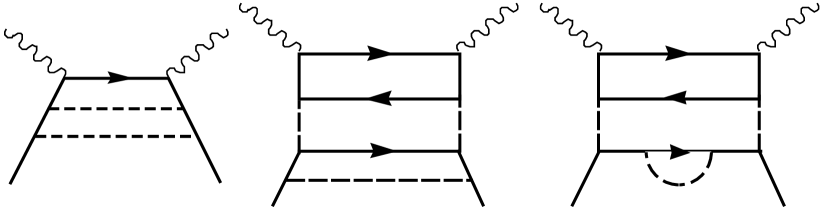
Figure 7:

Typical diagrams contributing to the constituent quark structure function with the two GS bosons. Notations are the same as those of Fig.1.

Due to factorization in the IMF, corrections from such diagrams are expressed by the already known splitting functions in most cases. We find the following two-pion contribution to the renormalization constant:

$$Z_{2\pi}=0.03\;,$$ (47)

which is about 10$\%$ of the total single GS boson contribution. We conclude that the inclusion of multi-pion Fock states is not expected to change our results significantly. The perturbative treatment of the GS boson cloud should therefore be justified.

We have also evaluated the GS boson correction to the chiral-odd $h_{1}(x)$ structure function. In comparison with the result for $g_{1}(x)$, where the CQ-GS boson splitting function $\Delta P$ is negative, we find a positive contribution to the $h_{1}(x)$ structure function. With inclusion of the renormalization effect, the transversity spin structure function for the $d$-quark is shown to be reduced significantly. We have found the relation $|\delta d|<|\Delta d|$, which seems to agree with recent lattice QCD results[13].

One may wonder how the QCD evolution of the tensor charge influences this discussion. In fact, the tensor charge decreases by the QCD evolution[31, 34]. However, even if one evolves from the very low scale $\mu^{2}=0.2\mbox{GeV}^{2}$ to a few $\mbox{GeV}^{2}$, the reduction of the tensor charge is at most $10\%$. We may therefore expect that the evolution does not change the relative magnitude of $\Delta q$ and $\delta q$ very much. We need some other dynamical mechanism to get $\Delta u<\delta u$ and $|\Delta d|>|\delta d|$, such as the GS boson dressing of the constituent quark, if the lattice result is confirmed.

Another interesting result has been obtained for the pion structure function. Sea quarks in the pion appear by direct emission of the GS bosons, while the nucleon case requires the second order process illustrated in Fig.1(b). This picture naturally gives a substantial enhancement of the sea quark distribution function in the pion. Such an enhancement can be checked in a future Drell-Yan experiment[40]. Our model calculations are done at the low energy scale $\sim 1\mbox{GeV}^{2}$, where the chiral quark model is supposed to make sense. To make a prediction for forthcoming experiments, we must carry out the $Q^{2}$ evolution from the low energy scale. However, the singlet evolution equation needs the gluon momentum fraction in the pion at the model scale, which we cannot estimate reliably at the moment.

We have studied aspects of constituent quark structure in deep inelastic processes. Non-perturbative features of the constituent quark, i.e. Goldstone boson fluctuations around the CQ, lead to screening effects and to characteristic changes of the CQ spin structure. Experimental tests of the nucleon transversity spin distribution function and the pion sea quark distribution will provide new insights into the role of the constituent quarks as quasi-particles.

In closing we mention that, recently, considerable interest has been focused on the possible experimental observation of such a “soft” pion cloud surrounding the nucleon. Semi-inclusive deep inelastic scattering processes with pions, nucleons or $\Delta$-isobar in the final state are studied as promising options by several authors[41].

Acknowledgments

K.S. would like to thank A. Hosaka for valuable conversations about the contribution of the pion cloud to the axial-vector coupling. This work is supported in part by the Alexander von Humboldt foundation and by BMBF.

References

- [1] See e.g., T. Muta, Foundations of Quantum Chromodynamics (World Scientific, Singapore, 1987)
-
[2]
M. Fukugita, Y. Kuramashi, M. Okawa and A. Ukawa,
Phys. Rev. Lett. 75 (1995) 2092
S.J. Dong, J.-F. Lagae and K.F. Liu, Phys. Rev. Lett. 75 (1995) 2096 - [3] R.L. Jaffe and G.G. Ross, Phys. Lett. B93 (1980) 313
-
[4]
C.J. Benesh and G.A. Miller, Phys. Rev. D36
(1987) 1344
A.W. Schreiber, A.I. Signal and A.W. Thomas, Phys. Rev. D44 (1991) 2653 -
[5]
W. Melnitchouk and W. Weise, Phys. Lett. B334 (1994) 275
S.A. Kulagin, W. Melnitchouk, T. Weigl and W. Weise, Nucl. Phys. A597 (1996) 515, and references therein -
[6]
M. Traini, L. Conci and U. Moschella, Nucl. Phys. A544
(1992) 731
M. Stratmann, Z. Phys. C60 (1993) 763
H.J. Weber, Phys. Rev. D49 (1994) 3160
V. Barone, T. Calarco and A. Drago, Phys. Lett. B390 (1997) 287
R. Jakob, P.J. Mulders and J. Rodrigues, hep-ph/9704335 - [7] F.E. Close and A.W. Thomas, Phys. Lett. B212 (1988) 227
- [8] H. Meyer and P.J. Mulders, Nucl. Phys. A528 (1991) 589
- [9] T. Shigetani, K. Suzuki and H. Toki, Phys. Lett. B308 (1993) 383; Nucl. Phys. A579 (1994) 413
- [10] A. Manohar and H. Georgi, Nucl. Phys. B234 (1984) 189
- [11] R.L. Jaffe and X. Ji, Nucl. Phys. B375 (1992) 527
-
[12]
E.J. Eichten, I. Hinchliffe and C. Quigg, Phys. Rev. D45 (1992) 2269
T.P. Cheng and L-.F. Li, Phys. Rev. Lett. 74 (1995) 2872 -
[13]
S. Aoki, M. Doui, T. Hatsuda and Y. Kuramashi,
Phys. Rev. D56 (1997) 433
M. Göckeler et al., DESY 96-152, hep-lat/9609039 - [14] S. Weinberg, Phys. Rev. Lett. 65 (1990) 1181
- [15] S.D. Drell, D.J. Levy and T.-M. Yan, Phys. Rev. D1 (1970) 1035
- [16] J. Speth and A.W. Thomas, preprint Jül-3283 (1996), and references therein
- [17] K. Suzuki, Phys. Lett. B368 (1996) 1
- [18] M. Glück, E. Reya and A. Vogt, Z. Phys. C53 (1992) 651
-
[19]
P. Amaudruz et al. (NMC Collaborations)
Phys. Rev. Lett. 66 (1991) 2716; M. Arneodo et al.,
Phys. Rev. D50 (1994) R1
For a recent review see: S. Kumano, preprint SAGA-HE-97-97, hep-ph/9702367 - [20] G. Piller, W. Ratzka and W. Weise, Z. Phys. A352 (1995) 427
-
[21]
D. Adams et al. (SMC collaborations), hep-ex/9702005
J. Ellis and M. Karliner, Phys. Lett. B341 (1995) 397 -
[22]
X. Ji, Phys. Rev. Lett. 78 (1997) 610
X. Ji, J. Tang and P. Hoodbhoy, Phys. Rev. Lett. 76 (1996) 740 -
[23]
H. Yabu, M. Takizawa and W. Weise, Z. Phys. A345 (1993) 193
K. Steininger and W. Weise, Phys. Rev. D48 (1993) 1433 -
[24]
Y. Nambu and G. Jona-Lasinio, Phys. Rev. 122 (1961) 345
For recent reviews see: T. Hatsuda and T. Kunihiro, Phys. Reports 247 (1994) 221; U. Vogl and W. Weise, Prog. Part. Nucl. Phys. 27 (1991) 195 - [25] For a recent review see: A. Hosaka and H. Toki, Phys. Reports 277 (1996) 65
-
[26]
R.L. Jaffe, Lectures at the 1979 Erice summer school,
Ettore Majorana
See also Section 5 of ref. [25]. -
[27]
V. Vento et al., Nucl. Phys. A345 (1980) 413
A.W. Thomas, S. Theberge and G.A. Miller, Phys. Rev. D24 (1981) 216
R. Tegen, M. Schedl and W. Weise, Phys. Lett. B125 (1983) 9 -
[28]
For reviews see e.g. A. Arima, Prog. Part. Nucl. Phys. 11
(1984) 53
I.S. Townes, Prog. Part. Nucl. Phys. 11 (1984) 91 - [29] B.L. Ioffe and A.Yu. Khodjiamirian, Phys. Rev. D51 (1995) 3373
-
[30]
J. Soffer, Phys. Rev. Lett. 74 (1995) 1992
G.R. Goldstein, R.L. Jaffe and X. Ji, Phys. Rev. D51 (1995) 3373 - [31] X. Artru and M. Mekhfi, Z. Phys. C45 (1990) 669 (1977) 298
- [32] K. Suzuki and T. Shigetani, TU-Munich preprint (1997), hep-ph/9709394, Nucl. Phys. A in press
- [33] H. He and X. Ji, Phys. Rev. D52 (1995) 2960, ibid D54 (1996) 6897
-
[34]
V. Barone, hep-ph/9703343;
W. Vogelsang, hep-ph/9706511 - [35] V. Barone, T. Calarco and A. Drago, Phys. Rev. D56 (1997) 527
- [36] J. Bartels, B.I. Ermolaev and M.G. Ryskin, Z. Phys. C70 (1996) 273, Z. Phys. C72 (1996) 627
- [37] R. Kirschner, L. Mankiewicz, A. Schäfer, L. Szymanowski, Z. Phys. C74 (1997) 501
- [38] P.J. Sutton, A.D. Martin, R.G. Roberts and W.J. Stirling, Phys. Rev. D45 (1992) 2349
- [39] M. Glück, E. Reya and A. Vogt, Z. Phys. C67 (1995) 433
- [40] J.T. Londergan, G.Q. Liu, E.N. Rodionov and A.W. Thomas, Phys. Lett. B361 (1995) 110
-
[41]
H. Holtmann, G. Levman, N.N. Nikolaev, A. Szczurek and J.
Speth, Phys. Lett. B338 (1994) 363;
W. Melnitchouk and A.W. Thomas, Z. Phys. A353 (1995) 311;
S. Baumgärtner, H.J. Pirner, K. Königsmann and B. Povh, Z. Phys. A353 (1996) 397