An Introduction to Solar Neutrino Research

PROLOGUE

In the first lecture, I describe the conflicts between the combined standard model predictions and the results of solar neutrino experiments. Here ‘combined standard model’ means the minimal standard electroweak model plus a standard solar model. First, I show how the comparison between standard model predictions and the observed rates in the four pioneering experiments leads to three different solar neutrino problems. Next, I summarize the stunning agreement between the predictions of standard solar models and helioseismological measurements; this precise agreement suggests that future refinements of solar model physics are unlikely to affect significantly the three solar neutrino problems. Then, I describe the important recent analyses in which the neutrino fluxes are treated as free parameters, independent of any constraints from solar models. The disagreement that exists even without using any solar model constraints further reinforces the view that new physics may be required. The principal conclusion of the first lecture is that the minimal standard model is not consistent with the experimental results that have been reported for the pioneering solar neutrino experiments.

In the second lecture, I discuss the possibilities for detecting “smoking gun” indications of departures from minimal standard electroweak theory. Examples of smoking guns are the distortion of the energy spectrum of recoil electrons produced by neutrino interactions, the dependence of the observed counting rate on the zenith angle of the sun (or, equivalently, the path through the earth to the detector), the ratio of the flux of neutrinos of all types to the flux of electron neutrinos (neutral current to charged current ratio), and seasonal variations of the event rates (dependence upon the earth-sun distance).

1 Introduction

Solar neutrino research entered a new era in April, 1996, when the Super-Kamiokande experiment[(1), (2)] began to operate. We are now in a period of precision, high-statistics tests of standard electroweak theory and of stellar evolution models.

In the previous era, solar neutrinos were detected by four beautiful experiments, the radiochemical Homestake chlorine experiment,[(3), (4)] the Kamiokande water Cerenkov experiment,[(5), (6)] and the two radiochemical gallium experiments, GALLEX[(7)] and SAGE.[(8)] In these four exploratory experiments, typically less than or of the order of 50 neutrino events were observed per year.

The pioneering experiments achieved the scientific goal which was set in the early 1960s,[(9), (10)] namely, “…to see into the interior of a star and thus verify directly the hypothesis of nuclear energy generation in stars.” We now know from experimental measurements, not just theoretical calculations, that the sun shines by nuclear fusion among light elements, burning hydrogen into helium.

Large electronic detectors will yield vast amounts of diagnostic data in the new era that has just begun. Each of the new electronic experiments is expected to produce of order several thousand neutrino events per year. These experiments, Super-Kamiokande,[(1), (2)] SNO,[(11)] and BOREXINO[(12)] will test the prediction of the minimal standard electroweak model[(13), (14), (15)] that essentially nothing happens to electron neutrinos after they are created by nuclear fusion reactions in the interior of the sun.

The four pioneering experiments—chlorine[(3), (4), (10)] Kamiokande[(5), (6)] GALLEX[(7)] and SAGE[(8)]—have all observed neutrino fluxes with intensities that are within a factors of a few of those predicted by standard solar models. Three of the experiments (chlorine, GALLEX, and SAGE) are radiochemical and each radiochemical experiment measures one number, the total rate at which neutrinos above a fixed energy threshold (which depends upon the detector) are detected. The sole electronic (non-radiochemical) detector among the initial experiments, Kamiokande, has shown that the neutrinos come from the sun, by measuring the recoil directions of the electrons scattered by solar neutrinos. Kamiokande has also demonstrated that the observed neutrino energies are consistent with the range of energies expected on the basis of the standard solar model.

Despite continual refinement of solar model calculations of neutrino fluxes over the past 35 years (see, e.g., the collection of articles reprinted in the book edited by Bahcall, Davis, Parker, Smirnov, and Ulrich[(16)]), the discrepancies between observations and calculations have gotten worse with time. All four of the pioneering solar neutrino experiments yield event rates that are significantly less than predicted by standard solar models.

These lectures are organized as follows. I first discuss in Section 2 the three solar neutrino problems. Next I discuss in Section 3 the stunning agreement between the values of the sound speed calculated from standard solar models and the values obtained from helioseismological measurements. Then I review in Section 4 recent work which treats the neutrino fluxes as free parameters and shows that the solar neutrino problems cannot be resolved within the context of the minimal standard electroweak model unless some solar neutrino experiments are incorrect. At this point, I summarize in Section 5 the main conclusions of the first lecture. I begin the second lecture by describing in Section 6 the new solar neutrino experiments and then answer in Section 7 the question: Why do physicists care about solar neutrinos? I present briefly in Section 8 and Section 9, respectively, the MSW solutions and the vacuum oscillation solutions that describe well the results of the four pioneering solar neutrino experiments. Finally, in Section 10 I describe the “smoking gun” signatures of physics beyond the minimal standard electroweak model that are being searched for with the new solar neutrino detectors. I summarize in Section 11 my view of where we are now in solar neutrino research.

I will concentrate in Lecture I on comparing the predictions of the combined standard model with the results of the operating solar neutrino experiments. By ‘combined’ standard model, I mean the predictions of the standard solar model and the predictions of the minimal standard electroweak theory.

We need a solar model to tell us how many neutrinos of what energy are produced per unit of time in the sun. Our physical intuition is not yet sufficiently advanced to know if we should be surprised by $10^{-2}$, by $10^{0}$, or by $10^{+2}$ neutrino-induced events per day in a chlorine tank the size of an Olympic swimming pool. Specifically, solar model calculations are required in order to predict the rate of nuclear fusion by the $pp$ chain (shown in Table 1 and the rate of fusion by the CNO reactions (originally favored by H. Bethe in his epochal study of nuclear fusion reactions). In a modern standard solar model, about $99$% of the energy generation is produced by reactions in the $pp$ chain. The most important neutrino producing reactions (cf. Table 1) are the low energy $pp$, $pep$, and the ⁷Be neutrinos, and the higher energy ⁸B neutrinos.

Table 1: The Principal Reactions of the $pp$ Chain

Reaction	Reaction	Neutrino Energy
Number		(MeV)
1	$\phantom{{}^{3}}p+p\to{\rm{}^{2}H}+e^{+}+\nu_{e}$	0.0 to 0.4
2	$\phantom{{}^{8}}p+e^{-}+p\to{\rm{}^{2}H}+\nu_{e}$	1.4
3	${\rm{}^{2}H}+p\to{\rm{}^{3}He}+\gamma$
4	${\rm{}^{3}He}+{\rm{}^{3}He}\to{\rm{}^{4}He}+2p$
	or
5	${\rm{}^{3}He}+{\rm{}^{4}He}\to{\rm{}^{7}Be}+\gamma$
	then
6	$\phantom{{}^{3}}e^{-}+{\rm{}^{7}Be}\to{\rm{}^{7}Li}+\nu_{e}$	0.86, 0.38
7	${\rm{}^{7}Li}+p\to{\rm{}^{4}He}+{\rm{}^{4}He}$
	or
8	$\phantom{{}^{3}}p+{\rm{}^{7}Be}\to{\rm{}^{8}B}+\gamma$
9	${\rm{}^{8}B}\to{\rm{}^{8}Be}+e^{+}+\nu_{e}$	0 to 15

A particle physics model is required to predict what happens to the neutrinos after they are created, whether or not flavor content of the neutrinos is changed as they make their way from the center of the sun to detectors on earth. For the first part of our discussion, I assume that essentially nothing happens to the neutrinos after they are created. In particular, they do not oscillate or decay to neutrinos with a different lepton number or energy. This assumption is valid if minimal standard electroweak theory is correct. In the simplest version of standard electroweak theory, neutrinos are massless and neutrino flavors (the number of $\nu_{e}$ or $\nu_{m}u$ or $\nu_{t}au$) are separately conserved. The minimal standard electroweak model has had many successes in precision laboratory tests; modifications of this theory will be accepted only if incontrovertible experimental evidence forces a change.

We will see that this comparison between combined standard model and solar neutrino experiments leads to three different discrepancies between the calculations and the observations, which I will refer to as the three solar neutrino problems. In the next section, I will discuss each of these three problems.

This is not a review article. My goal is to describe where we stand in solar neutrino research and where we are going, not to systematically describe the published literature. Some of the relevant background is presented in the excellent lectures in this Summer School by M. Davier, H. Harari, K. Martens, and S. Wojciki. See my home page http://www.sns.ias.edu/${\scriptstyle\sim}$jnb for more complete information about solar neutrinos, including anotated viewgraphs, preprints, and numerical data. Additional introductory material at roughly the level presented here can be found in two other recently published lectures.[(17), (18)] I have used here some material from these earlier talks but unfortunately could not cover everything contained in the previous discussions.

2 Three Solar Neutrino Problems

Figure 1 shows almost everything currently known about the solar solar neutrino problems.

The figure compares the measured and the calculated event rates in the four pioneering experiments, revealing three discrepancies between the experimental results and the expectations based upon the combined standard model. As we shall see, only the first of these discrepancies depends sensitively upon predictions of the standard solar model.

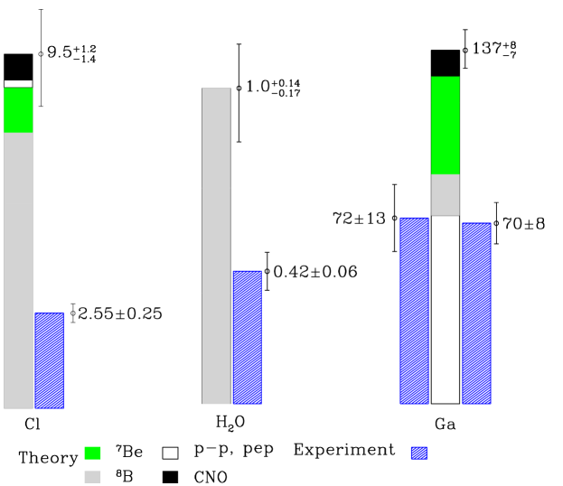
Figure 1: Comparison of measured rates and standard-model predictions for four solar neutrino experiments.

2.1 Problem 1. Calculated versus Observed Absolute Rate

The first solar neutrino experiment to be performed was the chlorine radiochemical experiment, which detects electron neutrinos that are more energetic than $0.81$ MeV. After more than 25 years of the operation of this experiment,[(4)] the measured event rate is $2.55\pm 0.25$ SNU which is a factor $\sim 3.6$ less than is predicted by the most detailed theoretical calculations, $9.5_{-1.4}^{+1.2}$ SNU.[(19), (20)] A SNU is a convenient unit to describe the measured rates of solar neutrino experiments: $10^{-36}$ interactions per target atom per second. Most of the predicted rate in the chlorine experiment is from the rare, high-energy ⁸B neutrinos, although the ⁷Be neutrinos are also expected to contribute significantly. According to standard model calculations, the $pep$ neutrinos and the CNO neutrinos (for simplicity not discussed here) are expected to contribute less than 1 SNU to the total event rate.

This discrepancy between the standard model calculations and the observations for the chlorine experiment was, for more than two decades, the only solar neutrino problem. I shall refer to the chlorine disagreement as the “first” solar neutrino problem.

2.2 Problem 2. Incompatibility of Chlorine and Water (Kamiokande) Experiments

The second solar neutrino problem results from a comparison of the measured event rates in the chlorine experiment and in the Japanese water Cerenkov experiment, Kamiokande. The water experiment detects higher-energy neutrinos, those with energies above $7$ MeV, by neutrino-electron scattering: $\nu~{}+~{}e~{}\longrightarrow\nu~{}+~{}e.$ According to the standard solar model, ⁸B beta decay is the only important source of these higher-energy neutrinos.

The Kamiokande experiment shows that the observed neutrinos come from the sun. The electrons that are scattered by the incoming neutrinos recoil predominantly in the direction of the sun-earth vector; the relativistic electrons are observed by the Cerenkov radiation they produce in the water detector.

In addition, the Kamiokande experiment measures the energies of individual scattered electrons and provides information about the energy spectrum of the incident solar neutrinos. The observed spectrum of electron recoil energies is consistent with that expected from ⁸B neutrinos. However, small angle scattering of the recoil electrons in the water prevents the angular distribution from being determined well on an event-by-event basis, which limits the constraints the experiment places on the incoming neutrino energy spectrum.

The event rate in the Kamiokande experiment is determined by the same high-energy ⁸B neutrinos that are expected, on the basis of the combined standard model, to dominate the event rate in the chlorine experiment. Solar physics changes the shape of the ⁸B neutrino spectrum by only 1 part in $10^{5}$ (see Ref. 21). Therefore, we can calculate the rate in the chlorine experiment that is produced by the ⁸B neutrinos observed in the Kamiokande experiment (above 7 MeV). This partial (⁸B) rate in the chlorine experiment is $3.2\pm 0.45$ SNU, which exceeds the total observed chlorine rate of $2.55\pm 0.25$ SNU.

Comparing the rates of the Kamiokande and the chlorine experiments, one finds that the best-estimate net contribution to the chlorine experiment from the $pep$, ⁷Be, and CNO neutrino sources is negative: $-0.66\pm 0.52$ SNU. The standard model calculated rate from $pep$, ⁷Be, and CNO neutrinos is 1.9 SNU. The apparent incompatibility of the chlorine and the Kamiokande experiments is the “second” solar neutrino problem. The inference that is most often made from this comparison is that the energy spectrum of ${\rm{}^{8}B}$ neutrinos is changed from the standard shape by physics not included in the simplest version of the standard electroweak model.

2.3 Problem 3. Gallium Experiments: No Room for ⁷Be Neutrinos

The results of the gallium experiments, GALLEX and SAGE, constitute the third solar neutrino problem. The average observed rate in these two experiments is $70.5\pm 7$ SNU, which is fully accounted for in the standard model by the theoretical rate of $73$ SNU that is calculated to come from the basic $pp$ and $pep$ neutrinos (with only a 1% uncertainty in the standard solar model $pp$ flux). The ⁸B neutrinos, which are observed above $7.5$ MeV in the Kamiokande experiment, must also contribute to the gallium event rate. Using the standard shape for the spectrum of ${\rm{}^{8}B}$ neutrinos and normalizing to the rate observed in Kamiokande, ${\rm{}^{8}B}$ contributes another $7$ SNU, unless something happens to the lower-energy neutrinos after they are created in the sun. (The predicted contribution is 16 SNU on the basis of the standard model.) Given the measured rates in the gallium experiments, there is no room for the additional $34\pm 4$ SNU that is expectedbahcall94 from ⁷Be neutrinos on the basis of standard solar models.

The seeming exclusion of everything but $pp$ neutrinos in the gallium experiments is the “third” solar neutrino problem. This problem is essentially independent of the previously-discussed solar neutrino problems, since this third problem depends strongly upon the $pp$ neutrinos, which are not observed in the other experiments. Moreover, the calculated $pp$ neutrino flux is approximately independent of solar models since it is closely related to the total luminosity of the sun.

The missing ⁷Be neutrinos cannot be explained away by any change in solar physics. The ⁸B neutrinos that are observed in the Kamiokande experiment are produced in competition with the missing ⁷Be neutrinos; the competition is between electron capture on ⁷Be versus proton capture on ⁷Be. Solar model explanations that reduce the predicted ${\rm{}^{7}Be}$ flux generically reduce much more, too much, the predicted ${\rm{}^{8}B}$ flux.

Figure 2: Predicted Solar Neutrino Gallium Event Rate Versus Year of Publication.gallium The figure shows the event rates for all of the standard solar model calculations that my colleagues and I have published. The cross sections from the recent paper by Bahcallgallium have been used in all cases to convert the calculated neutrino fluxes to predicted capture rates. The estimated $1\sigma$ uncertainties that are shown reflect just the uncertainties in the cross sections that are calculated in Ref 23. For the 35 years over which we have been calculating standard solar model neutrino fluxes, the historically lowest value (fluxes published in 1969) corresponds to $109.5$ SNU. This lowest-ever value is $5.6\sigma$ greater than the combined GALLEX and SAGE experimental result. If the points prior to 1992 are increased by $11$ SNU to correct for diffusion (this was not done in the figure), then all of the standard model theoretical capture rates since 1968 through 1997 lie in the range $120$ SNU to $141$ SNU.

The flux of ⁷Be neutrinos, $\phi({\rm{}^{7}Be})$, is independent of measurement uncertainties in the cross section for the nuclear reaction ${\rm{}^{7}Be}(p,\gamma)^{8}$B; the cross section for this proton-capture reaction is the most uncertain quantity that enters in an important way in the solar model calculations. The flux of ⁷Be neutrinos depends upon the proton-capture reaction only through the ratio

$$\phi({\rm{}^{7}Be})~{}\propto~{}{{R(e)}\over{R(e)+R(p)}},$$ (1)

where $R(e)$ is the rate of electron capture by ⁷Be nuclei and $R(p)$ is the rate of proton capture by ⁷Be. With standard parameters, solar models yield $R(p)\approx 10^{-3}R(e)$. Therefore, one would have to increase the value of the ${\rm{}^{7}Be}(p,\gamma)^{8}$B cross section by more than two orders of magnitude over the current best-estimate (which has an estimated uncertainty of $\sim$ 10%) in order to affect significantly the calculated ⁷Be solar neutrino flux. The required change in the nuclear physics cross section would also increase the predicted neutrino event rate by more than a factor of 100 in the Kamiokande experiment, making that prediction completely inconsistent with what is observed. (From time to time, papers have been published claiming to solve the solar neutrino problem by artificially changing the rate of the ⁷Be electron capture reaction. Equation (1) shows that the flux of ⁷Be neutrinos is independent of the rate of the electron capture reaction to an accuracy of better than 1%.)

Figure 2 shows the event rates for gallium solar neutrino experiments that are predicted by all of the standard solar model calculations that my colleagues and I have published in the 35 years, 1962-1997, in which we have been calculating solar neutrino fluxes. The historically lowest values (fluxes published in 1969) corresponds to 109.5 SNU, 5.6 sigma greater than the combined GALLEX and SAGE experimental result. If the predictions prior to 1992 are increased by 11 SNU to correct for diffusion (this was not done in the figure, but is required by helioseismological measurements, see below), then all of the standard model theoretical capture rates since 1968 lie in the range 120 SNU to 141 SNU. The solar model predictions for the gallium experiment are robust!

2.4 The bottom line

If we adopt the combined standard model, Figure 1 displays three solar neutrino problems: the smaller than predicted absolute event rates in the chlorine and Kamiokande experiments, the incompatibility of the chlorine and Kamiokande experiments, and the very low rate in the gallium experiment (which implies the absence of ⁷Be neutrinos although ⁸B neutrinos are observed).

I conclude that either: 1) at least three of the four pioneering solar neutrino experiments (the two gallium experiments plus either chlorine or Kamiokande) have yielded misleading results, or 2) physics beyond the minimal standard electroweak model is required to change the neutrino energy spectrum (or flavor content) after the neutrinos are produced in the center of the sun.

3 Comparison with Helioseismological
Measurements

Helioseismology has recently sharpened the disagreement between observations and the predictions of solar models with standard (non-oscillating) neutrinos. The helioseismological measurements demonstrate that the sound speeds predicted by standard solar models agree with extraordinary precision with the sound speeds of the sun inferred from helioseismological measurements.Basu96a ; Basu96b Because of the precision of this agreement, I am convinced that standard solar models cannot be in error by enough to make a major difference in the solar neutrino problems.

I will report here on some work that Marc Pinsonneault, Sarbani Basu, Jørgen Christensen-Dalsgaard, and I have done recently which demonstrates the precise agreement between the sound speeds in standard solar models and the sound speeds inferred from helioseismological measurement.BPBJCD

The square of the sound speed satisfies $c^{2}\mathrel{\raise 1.29167pt\hbox{$\propto$}\mkern-14.0mu\lower 2.58334pt\hbox{$\sim$}}T/\mu$, where $T$ is temperature and $\mu$ is mean molecular weight. The sound speeds in the sun are determined from helioseismology to a very high accuracy, better than $0.2$% rms throughout nearly all the sun. Thus even tiny fractional errors in the model values of $T$ or $\mu$ would produce measurable discrepancies in the precisely determined helioseismological sound speed

$${\delta c\over c}\simeq{1\over 2}\left({\delta T\over T}-{\delta\mu\over\mu}\right)\;.$$ (2)

The numerical agreement between standard predictions and helioseismological observations, which I will discuss in the following remarks, rules out solar models with temperature or mean molecular weight profiles that differ significantly from standard profiles. In particular, the helioseismological data essentially rule out solar models in which deep mixing has occurred (cf. PRL paperBPBJCD ) and argue against solar models in which the subtle effect of particle diffusion–selective sinking of heavier species in the sun’s gravitational field–is not included.

Figure 3 compares the sound speeds computed from two different solar models with the values inferredBasu96a ; Basu96b from the helioseismological measurements. The 1995, no diffusion, standard model of Bahcall and Pinsonneault (BP)BP95 is represented by the dotted line; the dark line represents our best solar modelBPBJCD which includes recent improvements in the OPAL equation of state and opacities, as well as helium and heavy element diffusion. For the standard model with diffusion, the rms discrepancy between predicted and measured sound speeds is $0.1$% (which is probably due in part to systematic uncertainties in the data analysis that produced the solar sound speeds).

Figure 3: Comparison of sound speeds predicted by different standard solar models with the sound speeds measured by helioseismology.BPBJCD There are no free parameters in the models. The figure shows the fractional difference, $\delta c/c$, between the predicted model sound speed and the measuredBasu96a ; Basu96b solar values as a function of radial position in the sun ($R_{\odot}$ is the solar radius). The dashed line refers to a modelBP95 in which diffusion is neglected and the dark line represents a standard model which includes diffusion and recent improvements in the OPAL equation of state and opacities.BPBJCD

Figure 3 shows that the discrepancies with the No Diffusion model are as large as $1$%. The mean squared discrepancy for the No Diffusion model is 22 times larger than for the best model with diffusion, OPAL EOS. If one supposed optimistically that the No Diffusion model were correct, one would have to explain why the diffusion model fits the data so much better. On the basis of Figure 3, we conclude that otherwise standard solar models that do not include diffusion, such as the model of Turck-Chièze and Lopez,TC93 are inconsistent with helioseismological observations. This conclusion is consistent with earlier inferences based upon comparisons with less complete helioseismological data, including the fact that the present-day surface helium abundance in a standard solar model agrees with observations only if diffusion is included.BP95

Equation 2 and Figure 3 imply that any changes $\delta T/T$ from the standard model values of temperature must be almost exactly canceled by changes $\delta\mu/\mu$ in mean molecular weight. In the standard solar model, $T$ and $\mu$ vary, respectively, by a factor of $53$ and by $43$% over the entire range for which $c$ has been measured and by $1.9$ and $39$% over the energy producing region. It would be an extraordinary coincidence if nature chose $T$ and $\mu$ profiles that individually differ markedly from the standard model but have the same ratio everywhere that they have in the standard model. There is no known reason why the large variation in $T$ should be finely tuned to the smaller variation in $\mu$. In the absence of a cosmic conspiracy, I conclude that the fractional differences between the solar temperature and the model temperature, $\delta T/T$, or the fractional differences between mean molecular weights, $\delta\mu/\mu$, are of similar magnitude to $\delta c^{2}/c^{2}$, i.e. (using the larger rms error, $0.002$, for the solar interior),

$$|\delta T/T|,~{}|\delta\mu/\mu|~{}\mathrel{\raise 1.29167pt\hbox{$<$}\mkern-14.0mu\lower 2.58334pt\hbox{$\sim$}}~{}0.004.$$ (3)

How significant for solar neutrino studies is the agreement between observation and prediction that is shown in Figure 3? The calculated neutrino fluxes depend upon the central temperature of the solar model approximately as a power of the temperature, ${\rm Flux}\propto T^{n}$, where for standard models the exponent $n$ varies from $n\sim-1.1$ for the $pp$ neutrinos to $n\sim+24$ for the ⁸B neutrinos.BU96 Similar temperature scalings are found for non-standard solar models.Castellani94 ; Castellani97 Thus, maximum temperature differences of $\sim 0.2\%$ would produce changes in the different neutrino fluxes of several percent or less, more than an order of magnitude less than requirednewphysics to ameliorate the solar neutrino problems discussed in Section 2.

Helioseismology rules out all solar models with large amounts of interior mixing (which homogenizes the mean molecular weight), unless finely-tuned compensating changes in the temperature are made. The mean molecular weight in the standard solar model with diffusion varies monotonically from $0.86$ in the deep interior to $0.62$ at the outer region of nuclear fusion ($R=0.25R\odot$) to $0.60$ near the solar surface. Any mixing model will cause $\mu$ to be constant and equal to the average value in the mixed region. At the very least, the region in which nuclear fusion occurs must be mixed in order to affect significantly the calculated neutrino fluxes.Bahcall89 ; EC68 ; BBU68 ; SS68 ; Schatzman69 Unless almost precisely canceling temperature changes are assumed, solar models in which the nuclear burning region is mixed ($R\mathrel{\raise 1.29167pt\hbox{$<$}\mkern-14.0mu\lower 2.58334pt\hbox{$\sim$}}0.25R_{\odot}$) will give maximum differences, $\delta c$, between the mixed and the standard model predictions, and hence between the mixed model predictions and the observations, of order

$${\delta c\over c}~{}=~{}{1\over 2}\left({{\mu-<\mu>}\over{\mu}}\right)~{}\sim~{}7\%~{}{\rm to}~{}10\%,$$ (4)

which is inconsistent with Figure 3.

4 “The Last Hope”: No Solar Model

The clearest way to see that the results of the four solar neutrino experiments are inconsistent with the predictions of the minimal standard electroweak model is not to use standard solar models at all in the comparison with observations. This is what Berezinsky, Fiorentini, and LissiaBerezinsky96 have termed “The Last Hope” for a solution of the solar neutrino problems without introducing new physics.

Let me now explain how model independent tests are made.

Let $\phi_{i}(E)$ be the normalized shape of the neutrino energy spectrum from one of the neutrino sources in the sun (e.g., ⁸B or $pp$ neutrinos). I have shownBahcall91 that the shape of the neutrino energy spectra that result from radioactive decays, ⁸B, ¹³N, ¹⁵O, and ¹⁷F, are the same to $1$ part in $10^{5}$ as the laboratory shapes. The $pp$ neutrino energy spectrum, which is produced by fusion has a slight dependence on the solar temperature, which affects the shape by about $1$%. The energies of the neutrino lines from ⁷Be and $pep$ electron capture reactions are also only shifted slightly, by about $1$% or less, because of the thermal energies of particles in the solar core.

Thus a test of the hypothesis that an arbitrary linear combination of the normalized standard neutrino spectra,

$$\Phi(E)~{}=~{}\sum_{i}\alpha_{i}\phi_{i}(E),$$ (5)

can fit the results of the neutrino experiments is equivalent to a test of minimal standard electroweak theory. One can choose the values of $\alpha_{i}$ so as to minimize the discrepancies with existing solar neutrino measurements and ignore all solar model information about the $\alpha_{i}$. One can add a constraint to Equation (5) that embodies the fact that the sun shines by nuclear fusion reactions that also produce the neutrinos. The explicit form of this luminosity constraint is

$$\frac{L_{\odot}}{4\pi r^{2}}=\sum_{j}\beta_{j}\phi_{j}~{},$$ (6)

where the eight coefficients, $\beta_{j}$, are determined by laboratory nuclear physics measurements and are given in Table VI of the paper by Bahcall and Krastev.BaKr

The first demonstration that the four pioneering experiments are by themselves inconsistent with the assumption that nothing happens to solar neutrinos after they are created in the core of the sun was by Hata, Bludman, and Langacker.Hata94 They showed that the solar neutrino data available by late 1993 were incompatible with any solution of Equations (5) and (6) at the 97% C.L.

In the most recent and complete published analysis in which the neutrino fluxes are treated as free parameters, Heeger and RobertsonHR96 showed that the data presented at the Neutrino ’96 Conference in Helsinki are inconsistent with Equations (5) and (6) at the 99.5% C.L. Even if they omitted the luminosity constraint, Equation (6), they found inconsistency at the 94% C.L. Similar results have been obtained by Hata and Langacker.HL97

It seems to me that these demonstrations are so powerful and general that there is very little point in discussing potential “solutions” to the solar neutrino problem based upon hypothesized non-standard scenarios for solar models.

5 Summary of the First Lecture

The combined predictions of the standard solar model and the minimal standard electroweak theory disagree with the results of the four pioneering solar neutrino experiments. The disagreement persists even if the neutrino fluxes are treated as free parameters, without reference to any solar model.

The solar model calculations are in excellent agreement with helioseismological measurements of the sound speed, providing further support for the inference that something happens to the solar neutrinos after they are created in the center of the sun.

Looking back on what was envisioned in 1964, I am astonished and pleased with what has been accomplished. In 1964, it was not clear that solar neutrinos could be detected. Now, they have been observed in five different experiments (including the results reported for Super-Kamiokande at this School) and the theory of stellar energy generation by nuclear fusion has been directly established. Moreover, helioseismology has confirmed to high precision predictions of the standard solar model, a possibility that also was not imagined in 1964. Particle theorists have shown that solar neutrinos can be used to study neutrino properties, another possibility that we did not envision in 1964. Much of the interest in the subject now stems from the unanticipated fact that the four pioneering experiments suggest that new neutrino physics may be revealed by solar neutrino measurements. We shall discuss in the next lecture some of the possibilities for detecting unique signatures of new physics with the powerful second generation of solar neutrino experiments that are now beginning to operate.

6 New Solar Neutrino Experiments

I would like to begin this second lecture by listing the new solar neutrino experiments. Table 2 shows the new experiments that are operating, under construction, or are being developed. You have already heard a lot about these experiments in the lectures by K. Martens.

Table 2: New Solar Neutrino Experiments

Collaboration	$\nu$’s	Detector	Technique	Beginning
				Date
Super-Kamiokande	${\rm{}^{8}B}$	22.5 kt ${\rm H_{2}O}$	$\nu$-$e$ scattering	April ’96
SNO	${\rm{}^{8}B}$	1 kt ${\rm D_{2}O}$	abs., nc disint.	Early ’98
GNO	$pp$, ${\rm{}^{7}Be}$ +…	30–100 t Ga	radiochemical	Early ’98
BOREXINO	${\rm{}^{7}Be}$	100 t liquid	$\nu$-$e$ scattering	’99
		scintillator
ICARUS	${\rm{}^{8}B}$	600 t liquid Ar	$\nu_{e}$ abs., TPC	’99
Iodine	${\rm{}^{7}Be,^{8}B}$,…	100 t iodine	radiochemical	’99
HELLAZ	$pp$, ${\rm{}^{7}Be}$	gaseous He	$\nu_{e}$-scattering	Develop.
			(TPC)
HERON	$pp$, ${\rm{}^{7}Be}$	liquid He	$\nu_{e}$-scattering	Develop.
			(superfluid, rotons)

I only want to add a few summary words. The Super-Kamiokande,Takita93 ; Totsuka96 SNO,McD94 and BOREXINOArp92 experiments all detect the recoil electrons produced by the neutrino interactions using Cerenkov detectors. The radiochemical experiments, GNO and Iodine (${\rm{}^{127}I}$),haxton87 ; cleveland detect neutrinos above a fixed threshold ($0.23$ MeV for GNO and $0.67$ MeV for Iodine) by counting the chemically extracted radioactive product (⁷¹Ge or ¹²⁷Xe) in a small proportional counter. All of the other experiments measure electronically energies associated with individual neutrino events. Among experiments that will operate before the year 2000, only GNO is sensitive to the low energy neutrinos from the fundamental $pp$ reaction and only BOREXINO can measure separately the flux of neutrinos from ⁷Be electron capture, the crucial ⁷Be neutrino line. SNO is the only experiment listed that can measure the total flux of neutrinos (of any flavor), which will be accomplished using the neutral current disintegration of deuterium. The neutrino interaction cross sections are well known (typical accuracy of order a few percent or better) for all of the detectors except ¹²⁷I.

7 Why do physicists care about solar neutrinos?

Solar neutrinos are of interest to physicists because they can be used to perform unique particle physics experiments. Many physicists believe that solar neutrino experiments may in fact have already provided strong hints that at least one neutrino type has a non-zero mass and that electron flavor (or the number of electron-type neutrinos) may not be conserved.

For some of the theoretically most interesting ranges of masses and mixing angles, solar neutrino experiments are more sensitive tests for neutrino transformations in flight than experiments that can be carried out with laboratory sources. The reasons for this exquisite sensitivity are: 1) the great distance between the beam source (the solar interior) and the detector (on earth); 2) the relatively low energy (MeV) of solar neutrinos; and 3) the enormous path length of matter ($\sim 10^{11}{\rm gm~{}cm^{-2}}$) that neutrinos must pass through on their way out of the sun.

One can quantify the sensitivity of solar neutrinos relative to laboratory experiments by considering the proper time that would elapse for a finite-mass neutrino in flight between the point of production and the point of detection. The elapsed proper time is a measure of the opportunity that a neutrino has to transform its state and is proportional to the ratio, $R$, of path length divided by energy:

$${\rm Proper~{}Time}~{}\propto~{}R=~{}{\rm{Path~{}Length}\over{Energy}}.$$ (7)

Future accelerator experiments with multi-GeV neutrinos may reach a sensitivity of $R={\rm 10^{2}~{}km~{}GeV^{-1}}$. Reactor experiments have already reached a level of sensitivity of $R={\rm 10^{2.5}~{}km~{}GeV^{-1}}$ for neutrinos with MeV energieschooz and are expected to improve to ${\rm 10^{4}~{}km~{}GeV^{-1}}$. Solar neutrino experiments, because of the enormous distance between the source (the interior of the sun) and the detector (on earth) and the relatively low energies ($1$ MeV to $10$ MeV) of solar neutrinos involve much larger values of neutrino proper time,

$$R({\rm solar})={{{10^{8}}\over{10^{-3}}}~{}{\left(\rm{km}\over{GeV}\right)}~{}\sim~{}10^{11}~{}{\left(\rm{km}\over{GeV}\right)}}.$$ (8)

Because of the long proper time that is available to a neutrino to transform its state, solar neutrino experiments are sensitive to very small neutrino masses that can cause neutrino oscillations in vacuum. Quantitatively,

$$m_{\nu}({\rm solar~{}level~{}of~{}sensitivity})\sim 10^{-6}{\rm eV~{}to}~{}10^{-5}{\rm eV}~{}~{}{\rm\left(vacuum~{}oscillations\right)},$$ (9)

provided the electron neutrino that is created by beta-decay contains appreciable portions of at least two different neutrino mass eigenstates (i.e., the neutrino mixing angle is relatively large). Direct laboratory experiments have achieved a sensitivity to electron neutrino masses of order a few eV. Over the next several years, the sensitivity of the laboratory experiments may be improved by an order of magnitude or more.

Resonant neutrino oscillations, which may be induced by neutrino interactions with electrons in the sun (the famous Mikheyev-Smirnov-Wolfenstein, MSW,msw effect), can occur even if the electron neutrino is almost entirely composed of one neutrino mass eigenstate (i.e., even if the mixing angles between $\nu_{e}$ and $\nu_{\mu}$ and between $\nu_{e}$ and $\nu_{\tau}$ neutrinos are tiny). Standard solar models indicate that the sun has a high central density, $\rho({\rm central})\sim 1.5\times 10^{2}~{}{\rm gm~{}cm^{-3}}$, which allows even very low energy ($<1$ MeV) electron neutrinos to be resonantly converted to the more difficult to detect $\nu_{\mu}$ or $\nu_{\tau}$ neutrinos by the MSW effect. Also, the column density of matter that neutrinos must pass through is large: $\int\rho dr\approx 2\times 10^{11}~{}{\rm gm~{}cm^{-2}}$. The corresponding parameters for terrestrial, long-baseline experiments are:  a typical density of ${\rm 3~{}gm~{}cm^{-3}}$, and an obtainable column density of $\sim 2\times 10^{8}~{}{\rm gm~{}cm^{-2}}$.

Given the above solar parameters, the planned and operating solar neutrino experiments are sensitive to neutrino masses in the range

$$10^{-4}~{}{\rm eV}~{}\mathrel{\raise 1.29167pt\hbox{$<$}\mkern-14.0mu\lower 2.58334pt\hbox{$\sim$}}~{}m_{\nu}~{}\mathrel{\raise 1.29167pt\hbox{$<$}\mkern-14.0mu\lower 2.58334pt\hbox{$\sim$}}~{}10^{-2}~{}{\rm eV},$$ (10)

via matter-induced resonant oscillations (MSW effect).

The range of neutrino masses given by Equation (9) and Equation (10) is included in the range of neutrino masses that are suggested by attractive particle-physics generalizations of the minimal standard electroweak model, including left-right symmetry, grand-unification, and supersymmetry.

Both vacuum neutrino oscillations and matter-enhanced neutrino oscillations can change electron neutrinos to the more difficult to detect muon or tau neutrinos (or even, in principle, to sterile neutrinos). In addition, the likelihood that a neutrino will have its flavor changed may depend upon its energy, thereby affecting the shape of the energy spectrum of the surviving electron neutrinos. Future solar neutrino experiments will measure the shape of the recoil electron energy spectrum (produced via charged current absorption and by neutrino-electron scattering) and will also measure the ratio of the number of electron neutrinos to the total number of solar neutrinos (via neutral current reactions). These measurements, of the spectrum shape and of the ratio of electron-type to total number of neutrinos, will test the simplest version of the minimal standard electroweak model in which neutrinos are massless and do not oscillate. These tests are independent of solar model physics.

For simplicity in the following discussions of both MSW and vacuum oscillations, I will assume that only two types of neutrinos are mixed. A richer set of solutions can be obtained if this assumption is dropped (see, e.g., the lectures by H. Harari at this summer school or the paper by Folgi et al.,fogli97a both of which contain a useful set of further references).

8 Allowed MSW solutions

The most popular neutrino physics solution, the Mikheyev-Smirnov-Wolfenstein (MSW) effect,msw predicts several characteristic phenomena that are not expected if minimal standard electroweak theory is correct. The MSW effect explains solar neutrino observations as the result of conversions in the solar interior of $\nu_{e}$ produced in nuclear reactions to the more difficult to detect $\nu_{\mu}$ or $\nu_{\tau}$.

Potentially decisive signatures of new physics that are suggested by the MSW effect include observing that the sun is brighter in neutrinos at night (the ‘earth regeneration effect’), earthreg ; BaltzW ; BaltzW2 detecting distortions in the incident solar neutrino energy spectrum,elspectJ and observing that the flux of all types of neutrinos exceeds the flux of just electron neutrinos.chen A demonstration that any of these phenomena exists would provide evidence for physics beyond the minimal standard electroweak model. I shall discuss in the next section the possibilities for detecting each of these signatures within the context of “The Search for Smoking Guns.”

Including the earth regeneration effect, Plamen Krastev and IBK97 have calculated the expected one-year average event rates as functions of the neutrino oscillation parameters, $\Delta m^{2}$ (the difference in squared neutrino masses), and $\sin^{2}2\theta$ (where $\theta$ is the mixing angle between $\nu_{e}$ and the mass eigenstate that $\nu_{e}$ most resembles), for all four operating experiments which have published results from their measurements of solar neutrino event rates. Specifically, the experiments included are the Homestake chlorine experiment, Kamiokande, GALLEX and SAGE. We take into account the known threshold and cross-sections for each detector. In the case of Kamiokande, we also take into account the known energy resolution (20%, $1\sigma$, at electron energy 10 MeV) and trigger efficiency function.Kam For similar calculations and related references, see, e.g., the papers by Maris and Petcovmaris and Lisi and Montanino.lisi97

We first calculate the one year average survival probability, $\bar{P}_{SE}$, for a large number of values of $\Delta m^{2}$ and $\sin^{2}2\theta$. Then we compute the corresponding one year average event rates in each detector. We perform a $\chi^{2}$ analysis taking into account theoretical uncertainties and experimental errors. We obtain allowed regions in $\Delta m^{2}$ - $\sin^{2}2\theta$ parameter space by finding the minimum $\chi^{2}$ and plotting contours of constant $\chi^{2}=\chi^{2}_{min}+\Delta\chi^{2}$ where $\Delta\chi^{2}=5.99$ for 95% C.L. and 9.21 for 99% .

The best fit is obtained for the small mixing angle (SMA) solution:

$$\Delta m^{2} = 5.0\times 10^{-6}{\rm eV}^{2},$$

$$\sin^{2}2\theta = 8.7\times 10^{-3},$$ (11)

which has a $\chi^{2}_{\rm min}=0.25$. There are two more local minima of $\chi^{2}$. The best fit for the well known large mixing angle (LMA) solution occurs at

$$\Delta m^{2} = 1.3\times 10^{-5}{\rm eV}^{2},$$

$$\sin^{2}2\theta = 0.63,$$ (12)

with $\chi^{2}_{\rm min}=1.1$. There is also a less probable solution,krastev93 ; BaltzW3 which we refer to as the LOW solution (low probability, low mass), at

$$\Delta m^{2} = 1.1\times 10^{-7}{\rm eV}^{2},$$

$$\sin^{2}2\theta = 0.83.$$ (13)

with $\chi^{2}_{\rm min}=6.9$. The LOW solution is acceptable only at 96.5% C.L.

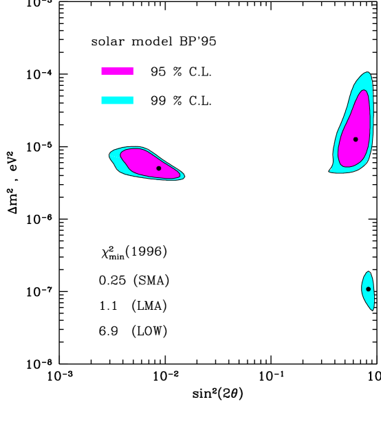
Figure 4: Allowed MSW solutions with regeneration.BK97 The allowed regions are shown for the neutrino oscillation parameters $\Delta m^{2}$ and $\sin^{2}2\theta$. The C.L. for the outer regions is 99% and the C. L for the inner regions is 99% (only applies to the LMA and SMA solutions). The data used here are from the Homestake chlorine,cleveland98 ; homestake Kamiokande,Suzuki95 ; kamioka GALLEX,Ansel95 ; GALLEX and SAGEAbdur94 ; SAGE experiments. The solar model used is the best standard model of Bahcall and Pinsonneault (1995) with helium and heavy element diffusion.BP95 The points where $\chi^{2}$ has a local minimum are indicated by a circle.

Figure 4 shows the allowed regions in the plane defined by $\Delta m^{2}$ and $\sin^{2}2\theta$. The C.L. is 95% for the allowed regions of the SMA and LMA solutions and 99% for the LOW solution. The black dots within each allowed region indicate the position of the local best-fit point in parameter space. The results shown in Fig. 4 were calculated using the predictions of the 1995 standard solar model of Bahcall and Pinsonneault,BP95 which includes helium and heavy element diffusion; the shape of the allowed contours depends only slightly upon the assumed solar model (see Fig. 1 of (Ref. 37).

The predicted $\nu-e$ scattering rates for the ${\rm 0.86~{}MeV~{}^{7}Be}$ line (which will be studied by BOREXINOArp92 ) relative to the Bahcall and Pinsonneault 1995 standard model BP95 are: $0.22^{+0.18}_{-0.00}$ (SMA), $0.54^{+0.17}_{-0.16}$ (LMA), and $0.54^{+0.08}_{-0.07}$ (LOW). The SMA and LMA ranges correspond to 95% C.L. and the LOW range is 99% C.L.

Figure 5: Survival probabilities for MSW solutions.BK97 The figure presents the survival probabilities for a $\nu_{e}$ created in the sun to remain a $\nu_{e}$ upon arrival at the earth. The best-fit MSW solutions including regeneration in the earth are described in in the text. The full line refers to the average survival probabilities computed taking into account regeneration in the earth and the dotted line refers to calculations for the day-time that do not include regeneration. The dashed line includes regeneration at night. There are only slight differences between the computed regeneration probabilities for the detectors located at the positions of Super-Kamiokande, SNO and the Gran Sasso Underground Laboratory.

Figure 5 compares the computed survival probabilities for the day (no regeneration), the night (with regeneration), and the annual average. These results show that there are day-night shifts in the neutrino energy spectrum as well as in the total rate, i.e., the shape of the effective $\nu_{e}$ energy spectrum depends upon the solar zenith angle. The results in the figure refer to a detector at the location of Super-Kamiokande, but the differences are very small between the survival probabilities at the positions of Super-Kamiokande, SNO, and the Gran Sasso Underground Laboratory.

9 Vacuum Neutrino Oscillations

Historically, neutrino oscillations in vacuumpontecorvo was the first suggested particle-physics solution to what was then the single “solar neutrino problem”, the fact that the rate of occurrence of neutrino events in the chlorine detector was smaller than predicted by standard solar models and the assumption that nothing happened to the neutrinos after they were produced.

Figure 6: Allowed vacuum oscillation solutions. The allowed regions are shown at the 99% C.L. for the neutrino oscillation parameters $\Delta m^{2}$ and $\sin^{2}2\theta$. The data used here are from the Homestake chlorine,cleveland98 ; homestake Kamiokande,kamioka GALLEX,GALLEX and SAGESAGE experiments, and a preliminary report from the Super-Kamiokande experiment (see lectures in this volume). The solar model used is the best standard model of Bahcall and Pinsonneault (1995) with helium and heavy element diffusion.BP95 The point where $\chi^{2}$ has a local minimum are indicated by a circle. This figure was prepared by P. Krastev.

Figure 6 shows the allowed range of solutions for vacuum oscillations, taking account of the four pioneering solar neutrino experiments and preliminary results from Super-Kamiokande. This figure was prepared by Plamen Krastev as part of our ongoing collaboration with Alexei Smirnov. The calculations were performed using the same data and methods described in the previous section in connection with the discussion of allowed MSW solutions.

10 The Search for Smoking Guns

The new generation of solar neutrino experiments will carry out tests of minimal standard electroweak theory that are independent of solar models. These experiments are designed to have the capabilities of detecting unique signatures of new physics, such as finite neutrino mass and mixing of neutrino types. For brevity, I shall refer to tell-tale evidences of new physics as “smoking guns.”

I will base the discussion of MSW smoking guns on three papers by Plamen Krastev, Eligio Lisi, and myself.BK97 ; snoJE ; BKL97 Similar papers have been written by other authors (see, for example, references in our papers), but I use our work here because I am most familiar with the details of what we did and because I have easy access to our figures. Our results are generally more pessimistic (indicate less sensitivity to new physics) than most of the other published works. This is because we have included estimates of the systematic uncertainties in our simulations, whereas most other workers have only included statistical errors. I will base the discussion of vacuum oscillations on the papers by Fogli, Lisi, and Montanino,Fogli97 and Krastev and Petcov.KP93

I will begin by describing in outline form how we have determined preliminary estimates of the likely sensitivities of the new solar neutrino experiments. Given the data from the four pioneering experiments (Homestake chlorine, Kamiokande, GALLEX, and SAGE), we determine the best-fit parameters, and the range of allowed solutions (at a specified C.L.), for a given model of new neutrino physics (e.g., vacuum neutrino oscillations or the MSW effect). Then we calculate the expected rates in the new experiments (Super-Kamiokande,Takita93 ; Totsuka96 SNO,McD94 BOREXINO,Arp92 ICARUS,revol HERON,lanou or HELLAZseguinot ) for all values of the new neutrino physics parameters that are suggested by the pioneering experiments. We take account of the characteristics of the new detectors that the experimental collaborations say are expected. For example, we include, in addition to statistical errors, the errors in the absolute energy determination of recoil electrons, the width and uncertainty of the energy resolution function, and the efficiency of detection, as well as uncertainties in the input theoretical quantities (like the shape of the intrinsic neutrino energy spectrum and uncertainties in neutrino interaction cross sections). We do not include the effects of background events, because the size of the backgrounds are not yet well known.

Full Monte Carlo simulations of the detectors will be necessary to determine accurately the sensitivities of each of the new experiments. These detailed simulations can only be done by the relevant experimental collaboration, since only the collaboration will have all the data required to make a realistic representation of how the detector operates.

In a survey of sensitivities, it is convenient to use the first two moments of the observable distributions predicted by different neutrino scenarios (e.g., the first two moments of the recoil electron energy spectrum or the zenith angle of the sun at the time of occurrence of neutrino events). My colleagues and I have shown by detailed analyses that the first two moments of the recoil energy spectrum or the solar zenith angle contain most of the important information.

10.1 Does the Sun Appear Brighter at Night
in Neutrinos?

The MSW solution of the solar neutrino problems requires that electron neutrinos produced in nuclear reactions in the center of the sun are converted to muon or tau neutrinos by interactions with solar electrons on their way from the interior of the sun to the detector on earth. The conversion in the sun is primarily a resonance phenomenon, which—for each neutrino energy—occurs at a specific density (for a specified neutrino mass difference).

During day-time, the higher-energy neutrinos arriving at earth are mostly $\nu_{\mu}$ (or $\nu_{\tau}$) with some admixture of $\nu_{e}$. At night-time, neutrinos must pass through the earth in order to reach the detector. As a result of traversing the earth, the fraction of the more easily detected $\nu_{e}$ increases because of the conversion of $\nu_{\mu}$ (or $\nu_{\tau}$) to $\nu_{e}$ by neutrino oscillations. For the small mixing angle MSW solution, interactions with electrons in the earth increase the effective mixing angle and enhance the conversion process. For the large mixing angle MSW solution, the conversion of $\nu_{\mu}$ (or $\nu_{\tau}$) to $\nu_{e}$ occurs by oscillations that are only slightly enhanced over vacuum mixing. This process of increasing in the earth the fraction of the neutrinos that are $\nu_{e}$ is called the “regeneration effect” and has the opposite effect to the conversion of $\nu_{e}$ to $\nu_{\mu}$ (or $\nu_{\tau}$) in the sun.

Because of the change of neutrino flavor in the earth, the MSW mechanism predicts that solar neutrino detectors should generally measure higher event rates at night than during day-time.

The regeneration effect is an especially powerful diagnostic of new physics since no difference is predicted between the counting rates observed during the day and at night (or, more generally, any dependence of the counting rate on the solar zenith angle) by such popular alternatives to the MSW effect as vacuum oscillations,pontecorvo magnetic moment transitions,okun or violations of the equivalence principle.gasperini

Figure 7: How many sigmas? The figure shows the sensitivity of Super-Kamiokande, SNO, ICARUS, BOREXINO and HERON/HELLAZ to the regeneration effect. Iso-sigma contours, statistical errors only, delineate the fractional percentage shifts of the first two moments of the angular distribution of events for an assumed 30000 observed events. Here $<\alpha>$ is the average solar zenith angle at the time of occurrence of solar neutrino events and $\sigma$ is the dispersion in the solar zenith angles. For all but the ICARUS experiment, the best-fit MSW solutions are indicated by black circles (SMA), squares (LMA), and triangles (LOW); the best-fit solutions are presented in Section 8. The error bars on the predicted moments correspond to $\Delta m^{2}$ and $\sin^{2}2\theta$ within allowed solution space at 95% C.L. (for Super-Kamiokande, SNO, and ICARUS) or 99% C.L. (BOREXINO and HERON/HELLAZ). For ICARUS, we have indicated the best-fit solutions by a transparent circle, square, or triangle. The best-fit SMA and LOW solutions for ICARUS and the LOW solution for SNO are all three close together at about $3\sigma$ from the no oscillation solution. In order to avoid too much crowding in the figure, we have not shown the theoretical uncertainties for ICARUS. This figure is Figure 9 of Bahcall and Krastev.BK97

Figure 7 summarizes the potential of the second generation of solar neutrino experiments for discovering new physics via the earth regeneration effect. The figure displays iso-sigma ellipses, statistical errors only, in the plane of the fractional percentage shifts of the first two moments, $\Delta\alpha/\alpha_{0}$ and $\Delta\sigma^{2}/\sigma_{0}^{2}$. Here $<\alpha>$ is the average solar zenith angle at the time of occurrence of solar neutrino events and $\sigma$ is the dispersion in the solar zenith angles.

Assuming a total number of events of 30000, (which corresponds to $\sim 5$ years of standard operation for Super-Kamiokande and $\sim 10$ years for SNO), we have computed the sampling errors on the first two moments as well as the correlation of the errors. The iso-sigma ellipses for the six detectors we consider here are centered around the undistorted zenith-angle exposure function for which, by definition, $\Delta\alpha=\Delta\sigma^{2}=0$. Figure 7 shows for each detector the predicted shifts of the first two moments in the SMA, LMA, and LOW solutions. The horizontal and vertical error-bars denote the spread in predicted values of the shifts in the first two moments, which are obtained by varying $\Delta m^{2}$ and $\sin^{2}2\theta$ within the 95% C.L. allowed (see Fig. 4) by the four pioneering solar neutrino experiments.

For Super-Kamiokande (SNO), the current best-fit parameters, $\Delta m^{2}$ and $\sin^{2}2\theta$, predict a $5\sigma$ ($6.5\sigma$) effect for the SMA solution and $13\sigma$ ($25\sigma$) effect for the LMA solution. Note that SNO is expected to require twice as much time to collect the same number of events as Super-Kamiokande. In the same amount of observing time, SNO and Super-Kamiokande are approximately equivalent for the SMA and Super-Kamiokande is significantly more efficient for the LMA.

The current best-estimate MSW solutions predict statistically significant deviations from the undistorted zenith-angle moments for the Super-Kamiokande, SNO, and ICARUS experiments (which are sensitive to the SMA and LMA solutions), but these experiments with the higher energy neutrinos are not sensitive to the deviations predicted by the LOW solution. However, Figure 7 shows that the BOREXINO and HERON/HELLAZ experiments are very sensitive to the LOW solution.

10.2 The Shape of the ⁸B Neutrino Energy Spectrum

The shape of the energy spectrum of neutrinos created by a specific continuum $\beta-$decay reaction is the same, to an accuracy of order 1 part in $10^{5}$, for neutrinos that are produced in the center of the sun and for neutrinos that are produced in a terrestrial laboratory, provided only that the minimal standard electroweak theory is correct.Bahcall91 The physical reason for this result is that the thermal velocities of ions in the solar interior are small compared to the velocity of light, $v^{2}/c^{2}\sim 10^{-6}$. First order corrections in $v/c$ vanish because the motions of the thermal ions are random. In fact, the largest correction ($\sim 10^{-5}$) to the shape of the energy spectrum arises from the general relativistic redshift.Bahcall91

Given this result, it follows that a measurement of the shape of the ⁸B neutrino energy spectrum is direct test of minimal standard electroweak theory. For small distortions, most of the available information is contained in the value of the average electron recoil energy, $<T_{e}>$ (see Appendix A of Bahcall and Lisi).snoJE If the distortion is large, it will show up clearly in any characterization, including the average recoil energy.

Figure 8: Values of the characteristic CC-shape variable, the average electron recoil energy $\langle T_{e}\rangle$ and of the CC/NC ratio, $R_{\rm CC}/R_{\rm NC}$, together with $3\sigma$ error bars. Here CC refers to $\nu_{e}$ absorption by deuterium with an electron being produced, which occurs via the charged current. The neutral current, NC, disintegration of the deuteron occurs with an equal cross section for all neutrino flavors ($\nu_{e}$, $\nu_{\mu}$, and $\nu_{\tau}$). Uncertainties due to the backgrounds are neglected. This is Figure 7 of the paper on SNO by Bahcall and Lisi.snoJE

For SNO, Figure 8a shows the predictions for $\langle T_{e}\rangle$ that follow from the best-estimate small angle (SMA) and large angle (LMA) MSW solutions, as well as the vacuum (vac) oscillation solution. The figure also shows the separate and combined $3\sigma$ errors expected from different sources; the efficiency error (labeled by a question mark) should be negligible if SNO works as expected.

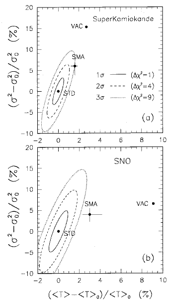
Figure 9: Spectral energy distortion. Iso-sigma contours in the plane of the fractional deviations of the first two spectral moments. (a) Super-Kamiokande experiment. (b) SNO experiment. The SMA solution can be distinguished at $\mathrel{\raise 1.03334pt\hbox{$>$}\mkern-14.0mu\lower 2.06668pt\hbox{$\sim$}}3\sigma$ from the standard (STD) case by both experiments. The crosses allow for variations of the SMA solution within the region favored at $95\%$ C.L. by the current experiments. See the text for details. The figure is Figure 4 from the paper of Bahcall, Krastev, and Lisi.BKL97

Figure 9 shows contours of equal standard deviations ($n$-sigma ellipses) in the plane of the $\langle T\rangle$ and $\sigma^{2}$ deviations of the spectrum that were computed for different neutrino scenarios. The contours are centered around the standard expectations (STD). Also shown are the representative best-fit points VAC and SMA. The point LMA is very close to STD and is not shown.

The cross centered at the SMA best-fit point indicates the solution space allowed at $95\%$ C.L. by the pioneering solar neutrino experiments. The deviations in $\langle T\rangle$ and $\sigma^{2}$ for the SMA solution are confined to a relatively small range. For vacuum oscillations, the range of deviations spanned by the whole region currently allowed at 95% C.L. by present data is much larger and is not indicated in Fig. 9. The statistical significance of the separation between the SMA and STD points in Fig. 9 is dominated by the fractional shift in $\langle T\rangle$ for both Super-Kamiokande and SNO. This is not surprising, since the SMA neutrino survival probability increases almost linearly with energy for $E_{\nu}>5$ MeV; this increase induces deformations of the electron recoil spectrum that are nearly linear in $T$ and are well represented by a shift in $\langle T\rangle$ .

The best-fit small mixing angle solution is separated by about $3\sigma$ or more from the standard solution for both Super-Kamiokande and SNO (see Fig. 9). The discriminatory power of the two experiments appears to be comparable for the SMA solution. The estimated total fractional errors of $\langle T\rangle$ and $\sigma^{2}$ in Super-Kamiokande are about a factor of two smaller than in SNO. However, the purely charged current (CC) interaction in SNO ($\nu_{e}$ absorption in deuterium) is a more sensitive probe of neutrino oscillations than a linear combination of charged current and neutral current (NC) interactions, as observed in Super-Kamiokande. In practice, the separation of charged current events and neutral current events (neutrino disintegration of the deuteron) in SNO will be affected by experimental uncertainties. We ignored misidentifications in our simulations.

How do the above results depend upon the energy threshold? The threshold is one of the most important quantities which experimentalists can hope to improve in order to increase the sensitivity of their detectors to distortion of the energy spectrum. We have determined by detailed calculations that the statistical significance of the SMA deviations in Figs. 4(a) and 4(b) decreases by about $0.6\sigma$ per 1 MeV increase in the energy threshold $T_{\rm min}$. These results are valid for both the SNO and the Super-Kamiokande detectors and include calculations for thresholds of $5$, $6$, and $7$ MeV.

10.3 The CC to NC Ratio

The bottom line for nearly all of the particle physics descriptions of what is happening in solar neutrino experiments is that a significant fraction of the $\nu_{e}$’s that are created in the interior of the sun are converted into $\nu_{\mu}$’s or $\nu_{\tau}$’s, either in the sun or on the way to the earth from the sun. The most direct test of this deviation from minimum standard electroweak theory is to measure the ratio of the flux of $\nu_{e}$’s (via a charged current, CC, interaction) to the flux of neutrinos of all types ($\nu_{e}+\nu_{\mu}+\nu_{\tau}$, determined by a neutral current, NC, interaction). The SNO collaboration is completing the construction of a 1000 ton heavy water detector in the Creighton Mine (Walden, Canada).SNOw The detector will measure the rates of the charged (CC) and neutral (NC) current reactions induced by solar neutrinos in deuterium:

$$\nu_{e}+d\rightarrow p+p+e^{-}\quad({\rm CC\ absorption})\quad,$$ (14)

$$\nu_{x}+d\rightarrow p+n+\nu_{x}\quad({\rm NC\ dissociation})\quad,$$ (15)

including the determination of the electron recoil energy in Equation (14). Only the more energetic ⁸B solar neutrinos are expected to be detected since the expected SNO threshold for CC events is an electron kinetic energy of about 5 MeV and the physical threshold for NC dissociation is the binding energy of the deuteron, $E_{b}=2.225$ MeV.

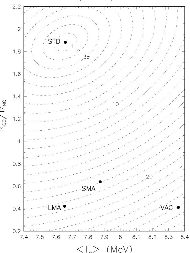
Figure 10: Iso-sigma contours $(\sigma=\sqrt{\chi^{2}})$ for the combined CC-shape and CC/NC test, for the representative oscillation cases discussed in the text. Uncertainties due to the backgrounds are neglected. For values of the iso-sigma distance ${\cal N}(\sigma)\gg 3$, the number of standard deviations is only a formal characterization; the tail of the probability distribution is not expected to be Gaussian for very large values of ${\cal N}(\sigma)$. This is Figure 8 of Bahcall and Lisi.snoJE

Figures 8a and 8b show the standard predictions for the average recoil energy, $\langle T_{e}\rangle$ (upper panel), and for the ratio, $R_{\rm CC}/R_{\rm NC}$ (lower panel), of CC $(\nu_{e})$ to NC (all flavors) together with the separate and combined $3\sigma$ errors. The values of $\langle T_{e}\rangle$ and $R_{\rm CC}/R_{\rm NC}$ for the different oscillation channels are also displayed.

Figure 10 shows the results of the combined tests (correlations included) in terms of iso-sigma contours in the plane $(\langle T_{e}\rangle,\,R_{\rm CC}/R_{\rm NC})$, where ${\cal N}(\sigma)=\sqrt{\chi^{2}}$. The three oscillation scenarios can be well separated from the standard case, but the vertical separation ($R_{\rm CC}/R_{\rm NC}$) is larger and dominating with respect to the horizontal separation ($\langle T_{e}\rangle$).

The error bars on the SMA point in Figs. 8–10 represent the range of values allowed at $95\%$ C.L. by a fit of the oscillation predictions to the four pioneering solar neutrino experiments;BK97 ; snoJE ; BKL97 the error bars are intended to indicate the effect of the likely range of the allowed oscillation parameters.

10.4 The Seasonal Dependence of the Neutrino Fluxes

For vacuum neutrino oscillations, the survival probability of $\nu_{e}$ at a distance $L$ from the sun is given byFrautschi69

$$P(E)=1-\sin^{2}2\theta\left({1.27\Delta m^{2}{\rm(eV)}L(m)\over E{\rm(MeV)}}\right),$$ (16)

where $E$ is the neutrino energy, $\Delta m^{2}$ is the neutrino squared mass-difference, and $\theta$ is the vacuum mixing angle. The ellipticity of the Earth’s orbit implies a striking signature of the oscillation phenomenon, namely, a dependence of the observed rate upon the instantaneous earth-sun distance, $L$ (in addition to the trivial geometric factor of $L^{-2}$). To a high accuracy, $L(t)=L_{0}\bigl{(}1-\epsilon\cos{{2\pi t}\over T}\bigr{)}$. where $L_{0}$ is $1$ AU, $T=1$ yr, and $\epsilon=0.0167$. The periodic dependence of the distance $L(t)$ upon time of the year implies a seasonal variation of the neutrino event rates.pontecorvo ; Fogli97 ; KP97 This variation is especially noticeable for neutrino masses in the range of $10^{-10}{\rm eV}^{2}$, which is consistent with some fraction (see Figure 2 of Bahcall and KrastevBaKr ) of the vacuum neutrino solutions that describe successfully the results of the pioneering solar neutrino experiments.

Among the second generation of experiments, the situation is most favorable for the BOREXINO experiment, since the events in this experiment are expected to be dominated by the ⁷Be (practically monoenergetic) neutrino line. Large effects can be anticipated for favorable cases for BOREXINO, but the effects will be reduced in the Super-Kamiokande and SNO experiments because the rates in these experiments average over neutrino energies. Fogli, Lisi, and MontaninoFogli97 propose a Fourier analysis of the neutrino signals for these experiments and show that with $10^{4}$ events and no appreciable backgrounds (a very optimistic assumption) there are currently-allowed vacuum neutrino solutions that would produce a $3\sigma$ effect in the Super-Kamiokande experiment and a $7\sigma$ effect in SNO.

11 Summary of Second Lecture

This is an incredibly exciting time to be doing solar neutrino research. There is a widespread feeling among people working in the field that we may be on the verge of making important discoveries about how neutrinos behave.

The greatest concern I have is that there are too few experiments. Looking back at the history of science, we see that it is necessary to have redundant experiments in order to test whether or not unrecognized systematic errors have crept into even the most careful measurements.

Only one experiment is planned that will measure a neutral current reaction (the SNO measurement of deuteron disintegration, see Equation 15). The neutral current to charged current ratio of fluxes determines most directly what we need to know in order to decide if new physics is occurring: the ratio of the total number of neutrinos to the number of $\nu_{e}$’s. Similarly, in order to test the astronomical predictions for the number of neutrinos created in the solar interior. we must know the total number of neutrinos that reach the earth in any flavor state.

Of the funded experiments, only BOREXINO has the planned sensitivity to detect the important ⁷Be neutrino line at $0.86$ MeV. The ⁷Be line is crucial for both the astronomical and the physical interpretations of the combined set of solar neutrino experiments (see for example the discussion in my reviewsbahcall96 ; bahcall97 ).

There are currently no funded projects for measuring individual events from the $pp$ neutrinos, although both HELLAX and HERON seem very promising. The low-energy $pp$ neutrinos constitute more than $90$% of the total solar neutrino flux in standard models. The radiochemical experiments, GALLEX, SAGE, and GNO, give us fundamental upper limits to the $pp$ flux at earth, but to exploit fully either the solar or the physics information encoded in the $pp$ neutrino flux we need measurements which determine the energy associated with each observed neutrino event.

We need more experiments, especially experiments sensitive to neutrinos with energies below $1$ MeV and experiments sensitive to neutral currents.

References

- (1) M. Takita, in Frontiers of Neutrino Astrophysics, edited by Y. Suzuki and K. Nakamura (Universal Academy Press, Inc., Tokyo, 1993), p. 147.
- (2) Y. Totsuka, to appear in the proceedings of the 18th Texas Symposium on Relativistic Astrophysics, December 15–20, 1996, Chicago, Illinois, edited by A. Olinto, J. Frieman, and D. Schramm (World Scientific, Singapore).
- (3) R. Davis, Jr., Prog. Part. Nucl. Phys. 32, 13 (1994).
- (4) B. T. Cleveland, T. Daily, R. Davis, Jr., J. R. Distel, K. Lande, C. K. Lee, P. S. Wildenhain, and J. Ullman, Astrophys. J. 495 (March 10, 1998).
- (5) Y. Suzuki (Kamiokande Collaboration), Nucl. Phys. B (Proc. Suppl.) 38, 54 (1995).
- (6) Y. Fukuda et al. (Kamioande Collaboration), Phys. Rev. Lett. 77, 1683 (1996).
- (7) P. Anselmann et al. (GALLEX collaboration), Phys. Lett. B 342, 440 (1995).
- (8) J. N. Abdurashitov et al. (SAGE Collaboration), Phys. Lett. B 328, 234 (1994).
- (9) J. N. Bahcall, Phys. Rev. Lett. 12, 300 (1964).
- (10) R. Davis, Jr., Phys. Rev. Lett. 12, 303 (1964).
- (11) A. B. McDonald, in Proceedings of the 9th Lake Louise Winter Institute, edited by A. Astbury et al. (World Scientific, 1994), p. 1.
- (12) C. Arpesella et al., BOREXINO Proposal, Vols. 1 and 2, edited by G. Bellini, R. Raghavan, et al. (Univ. of Milano, Milano, 1992).
- (13) S. L. Glashow, Nucl. Phys. 22, 579 (1961).
- (14) S. Weinberg, Phys. Rev. Lett. 19, 1264 (1967).
- (15) A. Salam, in Elementary Particle Theory, edited by N. Svartholm (Almqvist and Wiksells, Stockholm, 1968), p. 367.
- (16) Solar Neutrinos: The First Thirty Years, edited by J. N. Bahcall, R. Davis, Jr., P. Parker, A. Smirnov, and R. K. Ulrich (Addison Wesley, Reading, MA, 1995).
- (17) J. N. Bahcall, Astrophys. J. 467, 475 (1996).
- (18) J. N. Bahcall, in Unsolved Problems in Astrophysics, edited by J. N. Bahcall and J. P. Ostriker (Princeton University Press, Princeton, NJ, 1997), pp. 195–219.
- (19) J. N. Bahcall, M. H. Pinsonneault, S. Basu, and J. Christensen-Dalsgaard, Phys. Rev. Lett. 78, 171 (1997).
- (20) J. N. Bahcall, M. H. Pinsonneault, Rev. Mod. Phys. 67, 781 (1995).
- (21) J.N. Bahcall, Phys. Rev. D 44, 1644 (1991).
- (22) J. N. Bahcall, Phys. Lett. B 338, 276 (1994).
- (23) J. N. Bahcall, Phys. Rev. C, 56, No. 6, in press (1997); hep-ph/9710491.
- (24) S. Basu et al., Astrophys. J. 460, 1064 (1996).
- (25) S. Basu et al., Bull. Astron. Soc. India 24, 147 (1996).
- (26) S. Turck-Chièze and I. Lopez, Astrophys. J. 408, 347 (1993).
- (27) J. N. Bahcall and A. Ulmer, Phys. Rev. D 53, 4202 (1996).
- (28) V. Castellani, S. Degl’Innocenti, G. Fiorentini, and M. Lissia, Phys. Rev. D 50, 4749 (1994).
- (29) V. Castellani, S. Degl’Innocenti, G. Fiorentini, M. Lissia, and B. Ricci, Physics Reports 281, 310 (1997).
- (30) J. N. Bahcall and H. A. Bethe, Phys. Rev. Lett. 75, 2233 (1990); M. Fukugita, Mod. Phys. Lett. A 6, 645 (1991); M. White, L. Krauss, and E. Gates, Phys. Rev. Lett. 70, 375 (1993); V. Castellani, S. Degl’Innocenti, and G. Fiorentini, Phys. Lett. B 303, 68 (1993); N. Hata, S. Bludman, and P. Langacker, Phys. Rev. D 49, 3622 (1994); V. Castellani et al., Phys. Lett. B 324, 425 (1994); J. N. Bahcall, Phys. Lett. B 338, 276 (1994); S. Parke, Phys. Rev. Lett. 74, 839 (1995); G. L. Fogli and E. Lisi, Astropart. Phys. 3, 185 (1995); V. Berezinsky, G. Fiorentini, and M. Lissia, Phys. Lett. B 365, 185 (1996); A. Cumming and W. C. Haxton, Phys. Rev. Lett. 77, 4286 (1996).
- (31) J.N. Bahcall, Neutrino Astrophysics (Cambridge University Press, Cambridge, 1989).
- (32) D. Ezer and A. G. W. Cameron, Astrophys. Lett. 1, 177 (1968).
- (33) J. N. Bahcall, N. A. Bahcall, and R. K. Ulrich, Astrophys. Lett. 2, 91 (1968).
- (34) G. Shaviv and E. E. Salpeter, Phys. Rev. Lett. 21, 1602 (1968).
- (35) E. Schatzman, Astrophys. Lett. 3, 139 (1969); E. Schatzman and A. Maeder, Astron. Astrophys. 96, 1 (1981).
- (36) V. Berezinsky, G. Fiorentini, and M. Lissia, Phys. Lett. B 365, 185 (1996).
- (37) J. N. Bahcall and P. I. Krastev, Phys. Rev. D 53, 4211 (1996).
- (38) N. Hata, S. Bludman, and P. Langacker, Phys. Rev. D 49, 3622 (1994).
- (39) K. H. Heeger and R. G. H. Robertson, Phys. Rev. Lett. 77, 3720 (1996).
- (40) N. Hata and P. Langacker, Phys. Rev. D., in press (1997).
- (41) W. C. Haxton, Phys. Rev. Lett. 60, 768 (1987).
- (42) B. T. Cleveland et al., to appear in the proceedings of the Fourth International Solar Neutrino Conference, April 9–11, 1997, Heidelberg, Germany.
- (43) M. Apollonio et al. (CHOOZ Collaboration), hep-ex/9711002.
- (44) L. Wolfenstein, Phys. Rev. D 17, 2369 (1978); S. P. Mikheyev and A. Yu. Smirnov, Yad. Fiz. 42, 1441 (1985) [Sov. J. Nucl. Phys. 42, 913 (1985)]; Nuovo Cimento C 9, 17 (1986).
- (45) G. L. Fogli, E. Lisi, D. Montanino, and G. Scioscia, Phys. Rev. D 56, 4365 (1997).
- (46) S. P. Mikheyev and A. Yu. Smirnov, in ’86 Massive Neutrinos in Astrophysics and in Particle Physics, proceedings of the Sixth Moriond Workshop, edited by O. Fackler and Y. Trân Thanh Vân (Editions Frontières, Gif-sur-Yvette, 1986), p. 355; J. Bouchez et al., Z. Phys. C 32, 499 (1986); M. Cribier, W. Hampel, J. Rich, and D. Vignaud, Phys. Lett. B 182, 89 (1986); M. L. Cherry and K. Lande, Phys. Rev. D 36, 3571 (1987); S. Hiroi, H. Sakuma, T. Yanagida, and M. Yoshimura, Phys. Lett. B 198, 403 (1987); S. Hiroi, H. Sakuma, T. Yanagida, and M. Yoshimura, Prog. Theor. Phys. 78, 1428 (1987); A. Dar, A. Mann, Y. Melina, and D. Zajfman, Phys. Rev. D 35, 3607 (1988); M. Spiro and D. Vignaud, Phys. Lett. B 242, 279 (1990).
- (47) A. J. Baltz and J. Weneser, Phys. Rev. D 35, 528 (1987).
- (48) A. J. Baltz and J. Weneser, Phys. Rev. D 37, 3364 (1988).
- (49) H. Bethe, Phys. Rev. Lett. 56, 1305 (1986); S. P. Rosen and J. M. Gelb, Phys. Rev. D 34, 969 (1989); E. W. Kolb, M. S. Turner, and T. P. Walker, Phys. Lett. B 175, 478 (1986).
- (50) H. H. Chen, Phys. Rev. Lett. 55, 1534 (1985).
- (51) J. N. Bahcall and P. I. Krastev, Phys. Rev. C, 56, No. 5, 2839 (1997).
- (52) K. S. Hirata et al., Phys. Rev. D 44, 2241 (1991); see also Ref. 6.
- (53) M. Maris and S. T. Petcov, hep-ph/9705392.
- (54) E. Lisi and D. Montanino, Phys. Rev. D 56, 1792 (1997).
- (55) P. I. Krastev and S. T. Petcov, Phys. Lett. B 299, 99 (1993); G. L. Fogli, E. Lisi, and D. Montanino, Phys. Rev. D 54, 2048 (1996).
- (56) A. J. Baltz and J. Weneser, Phys. Rev. D 50, 5971 (1994); 51, 3960 (1995).
- (57) K. Lande and P. S. Wildenhain in Neutrino ’96, Proceedings of the 17th International Conference on Neutrino Physics and Astrophysics, Helsinki, Finland, 13–19 June 1996, edited by K. Huitu, K. Enqvist, and J. Maalampi (World Scientific, Singapore), pp. 25–37; see also, R. Davis, Prog. Part. Nucl. Phys. 32, 13 (1994); B. T. Cleveland et al., Nucl. Phys. B (Proc. Suppl.) 38, 47 (1995).
- (58) T. Kirsten et al. (GALLEX Collaboration), in Neutrino ’96, Proceedings of the 17th International Conference on Neutrino Physics and Astrophysics, Helsinki, Finland, 13–19 June 1996, edited by K. Huitu, K. Enqvist, and J. Maalampi (World Scientific, Singapore), pp. 3–13 ; for earlier results, see, P. Anselmann et al., Phys. Lett. B 327, 377 (1994); 342, 440 (1995); 357, 237 (1995).
- (59) V. Gavrin et al. (SAGE Collaboration), in Neutrino ’96, Proceedings of the 17th International Conference on Neutrino Physics and Astrophysics, Helsinki, Finland, 13–19 June 1996, edited by K. Huitu, K. Enqvist, and J. Maalampi (World Scientific, Singapore), pp. 14–24 ; see also, G. Nico et al., in Proceedings of the XXVII International Conference on High Energy Physics, Glasgow, Scotland, 1994, edited by P. J. Bussey and I. G. Knowles (Institute of Physics, Bristol, 1995), p. 965; J. N. Abdurashitov et al., Phys. Lett. B 328, 234 (1994).
- (60) V. N. Gribov and B. M. Pontecorvo, Phys. Lett. B 28, 493 (1969); B. Pontecorvo, J. Expl. Theor. Phys. 53, 1717 (1967).
- (61) J. N. Bahcall and E. Lisi, Phys. Rev. D 54, 5417 (1996).
- (62) J. N. Bahcall, P. I. Krastev, and E. Lisi, Phys. Rev. C 55, 494 (1997).
- (63) G. L. Folgi, E. Lisi, and D. Montanino, Phys. Rev. D 56, 4374 (1997).
- (64) P. I. Krastev and S. T. Petcov, Nucl. Phys. B 449, 605 (1993).
- (65) J. P. Revol, in Frontiers of Neutrino Astrophysics, edited by Y. Suzuki and K. Nakamura (Universal Academy Press, Inc., Tokyo, 1993), pp. 167–176.
- (66) R. E. Lanou, H. J. Baris, and G. M. Seidel, Phys. Rev. Lett. 58, 2498 (1987).
- (67) J. Seguinot, T. Ypsilantis, and A. Zichichi, Rep. No. LPC92-31 (College de France, Paris, 1992).
- (68) M. B. Volshin, M. I. Vysotsky, and L. B. Okun, Sov. Phys. JETP 64, 446 (1986).
- (69) M. Gasperini, Phys. Rev. D 38, 2635 (1988).
- (70) Updated information on the status of the SNO experiment can be retrieved from the following URL: http://snodaq.phy.queensu.ca/SNO/sno.html.
- (71) J. N. Bahcall and S. C. Frautschi, Phys. Lett. B 29, 623 (1969); S. Bilenky and B. Pontecorvo, Phys. Reports C 41, 225 (1978).
- (72) P. I. Krastev and S. T. Petcov, Phys. Lett. B 395, 69 (1997).