TTP97-42 UCSD/PHT 97-25
MPI/PhT/97-65 DESY 97-220
DTP/97/70 hep-ph/9711327
November 1997

1 Introduction

The total cross section for $e^{+}e^{-}$ annihilation into hadrons, $\sigma_{had}$, constitutes one of the most basic quantities of hadronic physics. It can be determined experimentally and calculated theoretically with high precision. It allows for a fundamental test of QCD and for a precise determination of its parameters, the strong coupling constant, and the quark masses. In addition, it provides the decisive input for an evaluation of the running QED coupling at high energies and for the hadronic contribution to the lepton anomalous magnetic moment. Perturbative QCD is expected to provide reliable predictions in the continuum, i.e. one or two GeV above the respective quark threshold and the respective resonance region. Calculations in the massless limit have been performed several years ago in ${\cal O}(\alpha_{s}^{2})$ [1] and ${\cal O}(\alpha_{s}^{3})$ [2] which we also refer to as NLO and NNLO (for a review see [3]). The effect of nonvanishing quark masses, $M_{Q}$, has been taken into account during the last years with the help of various quite different approaches: a large number of terms has been calculated in an expansion in $M_{Q}^{2}/s$ [4, 5], where $\sqrt{s}$ is the center of mass energy, and a subset of the diagrams has been evaluated analytically [6, 7]. Alternatively, the real and imaginary part of the polarization function $\Pi(q^{2})$ has been obtained by deriving analytical results for the expansions around $q^{2}=0$, for the limit $M_{Q}^{2}/q^{2}\ll 1$ and around $q^{2}=4M_{Q}^{2}$ and by using the analyticity of $\Pi(q^{2})$ to reconstruct the full function numerically [8]. The polarization function to order $\alpha_{s}^{2}$ for massive quarks is therefore under full control.

The previous papers were devoted to the technical aspects of the calculation and to systematic tests and cross checks. The present paper will be devoted to a compilation of the results in a simple and coherent form and to various phenomenological applications. It contains, in addition, the contribution from the double bubble diagram with a massive quark in the internal and the external fermion loop. In the phenomenological applications the dominant terms of order $\alpha_{s}^{3}$ in the massless approximation [2] plus $M_{Q}^{2}/s$ terms [9] will be included. This approach allows for a smooth interpolation between the high energy region where the formulae are accurate to NNLO order and the region closer to threshold where the results are valid to NLO order only.

The paper is organized as follows: a comprehensive account of all NLO results is presented in Section 2 for the sample case of the charm cross section. In Section 3 predictions for charm, bottom and top quark cross sections will be given. The sensitivity of the results towards a variation of the input parameters and the renormalization scale is investigated. In view of their stability in the regions away from the resonances the results for the cross sections can be used to predict the contributions of the charm and bottom continuum to the running of the QED coupling. A detailed study of this effect is performed in Section 4. The NLO perturbative results expanded for small velocities are an essential input for a calculation of the cross section very close to threshold, i.e. for energies comparable to or smaller than the Rydberg energy. In this region a resummation of leading and subleading terms of order $\pi\alpha_{s}/\beta$, where $\beta=\sqrt{1-4M_{Q}^{2}/s}$ is the velocity of the produced quarks, is required. Although we do not perform this resummation of singular terms in this paper, the essential ingredients from perturbation theory are presented in Section 5. Section 6 contains the summary and conclusion.

2 Predictions of order $\alpha_{s}^{2}$

In a first step the theoretical results shall be recalled which are required for the complete prediction of order $\alpha_{s}^{2}$ valid for energies sufficiently above the heavy quark threshold. The crucial ingredient in the present approach is the existence of a hierarchy of the quark masses. To be specific, let us consider the region above the charm and below the bottom threshold — the generalization to the other cases of interest being obvious. The energy is chosen sufficiently large, say above 5 GeV, to avoid the complications in the regime very close to the $c\bar{c}$ threshold (see Section 5). The $u$, $d$ and $s$ quark masses are neglected. Virtual bottom effects are treated through an expansion in $s/(4M_{b}^{2})$. This approximation is adequate in the full energy region under consideration, even for $s/(4M_{b}^{2})\to 1$ [6]. We are mainly interested in the region where $\sqrt{s}$ and $M_{c}$ are of comparable magnitude. It is thus convenient to identify the quark mass with the pole mass, a convention adopted throughout this paper.

In order $\alpha_{s}^{2}$ the contributions from different quark species to the vector current correlator can be distinguished and thus added incoherently — only “non–singlet terms” are present in this order. The singlet contribution, which starts in order $\alpha_{s}^{3}$, has been calculated for massless quarks and is small [2]. In the following we shall first recall the contributions arising from the electromagnetic current coupled to the light $u$, $d$ and $s$ quarks, and subsequently the charm contribution — the main subject of this work. We would like to stress, that the formulae, with the obvious replacements, are equally well applicable for $b\bar{b}$ or $t\bar{t}$ production above their respective thresholds (see Section 3).

1. The sum of the absorptive parts of one-, two- and three-loop diagrams with massless degrees of freedom (quarks or gluons) is given by [1]:

$$R_{\rm light}(s) = 3\sum_{i=u,d,s}Q_{i}^{2}\,\Bigg{\{}1+\frac{\alpha_{s}^{(4)}(\mu^{2})}{\pi}+\left(\frac{\alpha_{s}^{(4)}(\mu^{2})}{\pi}\right)^{2}\bigg{[}\frac{365}{24}-11\,\zeta(3)$$ (1)

$$\qquad\qquad\qquad\mbox{}+n_{\ell}\left(-\frac{11}{12}+\frac{2}{3}\,\zeta(3)\right)+\left(-\frac{11}{4}+\frac{1}{6}n_{\ell}\right)\ln\frac{s}{\mu^{2}}\bigg{]}\Bigg{\}}\,,$$

where $\zeta(3)\approx 1.2020569$ and $n_{\ell}=n_{f}-1$ is the number of massless quarks. The $\overline{\rm MS}$ coupling $\alpha_{s}^{(4)}$ is to be evaluated at the scale $\mu^{2}$. Anticipating our strategy to include the dominant $\alpha_{s}^{3}$ terms in the high energy region, the evolution of the strong coupling is governed by the three-loop beta function with $n_{f}=n_{\ell}+1$ active flavours, where $n_{f}=4$ is chosen for the sample case of charm quark production.

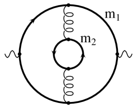
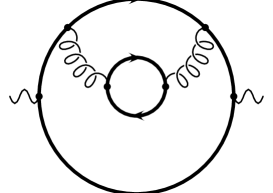
Figure 1: Fermionic double bubble diagrams with generic masses $m_{1}$ and $m_{2}$.

2. Charm quarks can be produced through the splitting of gluons, which in turn are radiated off $u$, $d$ or $s$ quarks. The analytic result for this cross section can be found in [6], the corresponding virtual corrections to light quark pair production were obtained earlier in [10] in the on-shell renormalization scheme. The sum gives rise to the following “double bubble” contribution (see Fig. 1 with $m_{1}=0,m_{2}=M_{c}$):

$$TC_{F}R_{qc}^{(2)} = 3\sum_{i=u,d,s}Q_{i}^{2}\,\frac{2}{3}\,\left(\rho^{V}(0,M_{c}^{2},s)+\rho^{R}(0,M_{c}^{2},s)+\frac{1}{4}\ln\frac{M_{c}^{2}}{\mu^{2}}\right)\,.$$ (2)

The functions $\rho^{V}(0,M_{c}^{2},s)$ and $\rho^{R}(0,M_{c}^{2},s)$ are given in [6]. The combination on the right hand side of Eq. (2) is well approximated by the leading terms in the high energy limit. This is demonstrated in Fig. 2, where the combination $\left(\rho^{V}(0,M_{c}^{2},s)+\rho^{R}(0,M_{c}^{2},s)+\frac{1}{4}\ln\frac{M_{c}^{2}}{s}\right)$ is shown, together with the leading terms of the high energy approximation ($\mu^{2}=s$)

$$\rho^{V}(0,M_{c}^{2},s)+\rho^{R}(0,M_{c}^{2},s)+\frac{1}{4}\ln\frac{M_{c}^{2}}{s}\,\,\,\stackrel{{\scriptstyle M_{c}^{2}/s\to 0}}{{\longrightarrow}}$$ (3)

$$\zeta(3)-\frac{11}{8}+\frac{M_{c}^{4}}{s^{2}}\left(-\frac{3}{2}\ln\frac{M_{c}^{2}}{s}-6\,\zeta(3)+\frac{13}{2}\right)+{\cal O}\left(\frac{M_{c}^{6}}{s^{3}}\right).$$

Note that the absence of $M_{c}^{2}$ terms could be inferred from general renormalization group considerations [9].

Figure 2: The function $\left(\rho^{V}(0,M_{c}^{2},s)+\rho^{R}(0,M_{c}^{2},s)+\frac{1}{4}\ln\frac{M_{c}^{2}}{s}\right)$ as described in the text. Solid line: exact result; dash-dotted line: constant and quadratic terms only; dashed line: including terms up to order $M_{c}^{4}/s^{2}$ corrections (from [6]). The scale $\mu^{2}=s$ has been adopted.

3. Double bubble diagrams with external $u$, $d$, $s$ (or $c$) and internal $b$ quarks decouple in the limit $s/(4M_{b}^{2})\ll 1$. For vanishing external quark mass an analytic result is available [10], closely related to $\rho^{V}(0,M_{c}^{2},s)$ given above. It is well approximated by the leading term in the $s/M_{b}^{2}$ expansion [11, 12] — even up to $s=4M_{b}^{2}$:

$$TC_{F}\delta R_{qb}^{(2)}=3\sum_{i=u,d,s}Q_{i}^{2}\,\frac{s}{4M_{b}^{2}}\,\bigg{[}\frac{8}{135}\ln\frac{M_{b}^{2}}{s}+\frac{176}{675}\bigg{]}\,.$$ (4)

These terms are numerically small.

The combination of all terms proportional to $\sum_{i=u,d,s}Q_{i}^{2}$ thus reads

$$R_{uds}(s) = R_{\rm light}+\left(\frac{\alpha_{s}^{(4)}(\mu^{2})}{\pi}\right)^{2}TC_{F}\left(R_{qc}^{(2)}(s)+\delta R_{qb}^{(2)}(s)\right).$$ (5)

$R_{uds}$ is separately renormalization group invariant and approaches $R_{\rm light}|_{n_{\ell}\to n_{f}}$ in the limit $M_{c}^{2}\ll s\ll M_{b}^{2}$.

Let us now proceed to the contributions arising from charm quarks coupled to the electromagnetic current. They will be cast into the form

$$R_{c} = Q_{c}^{2}\left(R_{c}^{(0)}+\frac{\alpha_{s}^{(4)}(\mu^{2})}{\pi}\,C_{F}\,R_{c}^{(1)}+\left(\frac{\alpha_{s}^{(4)}(\mu^{2})}{\pi}\right)^{2}\,R_{c}^{(2)}\,\right).$$ (6)

The lowest order terms are well known [13] and read

$$R_{c}^{(0)}\,\,=\,\,3\,\beta\frac{3-\beta^{2}}{2}, R_{c}^{(1)}\,\,=\,\,3\,\rho^{(1)},$$ (7)

where

$$\rho^{(1)} = \frac{\left(3-{\beta^{2}}\right)\,\left(1+{\beta^{2}}\right)}{2}\,\bigg{[}\,2\,\mbox{Li}_{2}(p)+\mbox{Li}_{2}({p^{2}})+\ln p\,\Big{(}2\,\ln(1-p)+\ln(1+p)\Big{)}\,\bigg{]}\,\,$$ (8)

$$\mbox{}-\beta\,(3-{\beta^{2}})\,\Big{(}2\,\ln(1-p)+\ln(1+p)\Big{)}$$

$$\mbox{}-\frac{\left(1-\beta\right)\,\left(33-39\,\beta-17\,{\beta^{2}}+7\,{\beta^{3}}\right)}{16}\,\ln p+\frac{3\,\beta\,\left(5-3\,{\beta^{2}}\right)}{8}\,,$$

with

$$p\,=\,\frac{1-\beta}{1+\beta}\,,\qquad\,\beta\,=\,\sqrt{1-4M_{c}^{2}/s}\,$$ (9)

and $\mbox{Li}_{n}(p)$ is the polylogarithmic function. In the limit $\beta\to 0$ $\rho^{(1)}$ behaves as follows:

$$\rho^{(1)} \stackrel{{\scriptstyle\beta\to 0}}{{\longrightarrow}} \frac{9}{2}\zeta(2)-6\beta+3\zeta(2)\beta^{2}+{\cal O}(\beta^{3}).$$ (10)

with $\zeta(2)=\pi^{2}/6$. In order $\alpha_{s}^{2}$ a variety of diagrams has to be considered.

4. The essential ingredients for an evaluation of the double bubble diagram with two charm quark loops (see Fig. 1 with $m_{1}=m_{2}=M_{c}$) can be found in [7]. The virtual corrections to the $c\bar{c}$ vertex contribute for $\sqrt{s}>2M_{c}$ and are known analytically [7]. The final state with four charm (anti–) quarks is strongly suppressed close to its threshold at $4M_{c}\approx 7$ GeV. The rate is given in terms of a two dimensional integral to be evaluated numerically. The combined contribution is thus written as

$$T\,C_{F}\,R_{cc}^{(2)} = 3\,\left(\frac{2}{3}\,\rho^{V}(M_{c}^{2},M_{c}^{2},s)+\frac{2}{3}\,\rho^{R}(M_{c}^{2},M_{c}^{2},s)+\frac{1}{6}\ln\frac{M_{c}^{2}}{\mu^{2}}\,\frac{4}{3}\,\rho^{(1)}\right)$$ (11)

where

$$\rho^{V}(M_{c}^{2},M_{c}^{2},s) = \frac{1}{6}\,\Bigg{[}\,\frac{3+10\beta^{2}-5\beta^{4}}{24}\,\ln^{3}p+\frac{-3+40\beta^{2}+16\beta^{4}-15\beta^{6}}{12\beta^{3}}\,\ln^{2}p$$ (12)

$$\quad+\bigg{(}\frac{-18+234\beta^{2}+167\beta^{4}-118\beta^{6}}{18\beta^{2}}+\frac{-3-10\beta^{2}+5\beta^{4}}{2}\,\zeta(2)\bigg{)}\ln p$$

$$\quad+\frac{-9+510\beta^{2}-118\beta^{4}}{9\beta}+\beta\,(-27+5\beta^{2})\,\zeta(2)\,\Bigg{]}$$

and

$$\rho^{R}(M_{c}^{2},M_{c}^{2},s)=\frac{1}{3}\,\int_{4M_{c}^{2}/s}^{(1-2M_{c}/\sqrt{s})^{2}}{\rm d}y\,\int_{4M_{c}^{2}/s}^{(1-\sqrt{y})^{2}}\frac{{\rm d}z}{z}\,\left(1+\frac{2M_{c}^{2}}{sz}\right)\sqrt{1-\frac{4M_{c}^{2}}{sz}}\,\,{\cal F}(y,z)\,,$$ (13)

with

$${\cal F}(y,z) := \frac{\frac{8M_{c}^{4}}{s^{2}}+\frac{4M_{c}^{2}}{s}(1-y+z)-(1-y+z)^{2}-2(1+z)y}{1-y+z}$$

$$\cdot\ln\frac{1-y+z-\sqrt{1-\frac{4M_{c}^{2}}{sy}}\,\Lambda^{1/2}(1,y,z)}{1-y+z+\sqrt{1-\frac{4M_{c}^{2}}{sy}}\,\Lambda^{1/2}(1,y,z)}$$

$$-\sqrt{1-\frac{4M_{c}^{2}}{sy}}\,\Lambda^{1/2}(1,y,z)\,\left[1+\frac{\frac{16M_{c}^{4}}{s^{2}}+\frac{8M_{c}^{2}}{s}+4\left(1+\frac{2M_{c}^{2}}{s}\right)z}{(1-y+z)^{2}-\left(1-\frac{4M_{c}^{2}}{sy}\right)\,\Lambda(1,y,z)}\,\right]\,,$$

$$\Lambda(1,y,z) := 1+y^{2}+z^{2}-2(y+z+yz)\,.$$ (15)

Note that $\rho^{R}(M_{c}^{2},M_{c}^{2},s)$ vanishes for $s\to 16M_{c}^{2}$. The function $\rho^{V}(M_{c}^{2},M_{c}^{2},s)$ vanishes for $s\to 4M_{c}^{2}$ and $\rho^{(1)}$ approaches the constant $3\pi^{2}/4$ in the same limit. Both are zero below $4M_{c}^{2}$. For small $\beta$ one obtains:

$$\rho^{V}(M_{c}^{2},M_{c}^{2},s) \stackrel{{\scriptstyle\beta\to 0}}{{\longrightarrow}} \left(\frac{22}{3}-4\zeta(2)\right)\beta+\left(-\frac{245}{54}+\frac{8}{3}\zeta(2)\right)\beta^{3}+{\cal O}(\beta^{5})\,.$$ (16)

$R_{cc}^{(2)}$ is shown in Fig. 3 as a function of $M_{c}^{2}/s$ in the range from 0 to 1/4. The contribution from four particle production $\rho^{R}(M_{c}^{2},M_{c}^{2},s)$ and the virtual correction $\rho^{V}(M_{c}^{2},M_{c}^{2},s)+\frac{1}{3}\rho^{(1)}\ln\frac{M_{c}^{2}}{s}$ are displayed separately as dashed and dotted lines, respectively, their sum is shown as a solid line. In the high energy limit the sum approaches (for $\mu^{2}=s$) a constant value:

$$\rho^{V}(M_{c}^{2},M_{c}^{2},s)+\rho^{R}(M_{c}^{2},M_{c}^{2},s)+\frac{1}{3}\rho^{(1)}\ln\frac{M_{c}^{2}}{s} \stackrel{{\scriptstyle M_{c}^{2}/s\to 0}}{{\longrightarrow}} \zeta(3)-\frac{11}{8}+{\cal O}\left(\frac{M_{c}^{2}}{s}\right)\,.$$ (17)

Fig. 3 demonstrates that for energies far above the four particle threshold, i.e. for $\sqrt{s}\gg 4M_{c}$, real and virtual contributions cancel to a large extent. For smaller energies, however, the (negative) virtual corrections become increasingly more important as the energy decreases down to the two particle threshold.

Figure 3: Second order contributions from double bubble diagrams with massive internal and external quarks of the same mass as a function of $M_{c}^{2}/s$. Dashed line: the real contribution $\rho^{R}(M_{c}^{2},M_{c}^{2},s)$; dotted line: the virtual correction $\rho^{V}(M_{c}^{2},M_{c}^{2},s)+\frac{1}{3}\rho^{(1)}\ln\frac{M_{c}^{2}}{\mu^{2}}$ for $\mu^{2}=s$; solid line: the sum of both.

The contributions from charm quarks coupled to the external current with internal massless quark or gluon lines are significantly more important. Their treatment is the main subject of this paper. Very close to threshold the Coulomb singularity has to be incorporated and the definition of the coupling has to be scrutinized. However, in a first step, the energy region will be considered where mass terms are important but Coulomb resummation is not yet required.

5. Let us start with double bubble diagrams with light internal quark loops (see Fig. 1 with $m_{1}=M_{c},m_{2}=0$). In the previous cases, Eqs. (2) and (11) with massive internal quark loops, the rates for real and virtual radiation could be given separately and no mass singularity was present. This differs from the case with vanishing internal quark mass: quadratic and linear mass logarithms arise in the individual cuts which can be cancelled by combining real and virtual emission and by adopting the $\overline{\rm MS}$ definition of the coupling constant. The analytical result has been obtained in [7] (see also [14]). For completeness we recall the result for $n_{\ell}$ light quark species:

$$n_{\ell}\,T\,C_{F}\,R_{cq}^{(2)} = 3\,\frac{2}{3}\,n_{\ell}\left(-\,\frac{1}{3}\,\bigg{[}\ln\frac{\mu^{2}}{s}+\frac{5}{3}-\ln 4\bigg{]}\,\rho^{(1)}+\delta^{(2)}\right)\,,$$ (18)

where $\rho^{(1)}$ is given in Eq. (8) and

$$\delta^{(2)}\,=\,-\,\frac{\left(3-{{\beta}^{2}}\right)\,\left(1+{{\beta}^{2}}\right)}{6}\,$$ (19)

$$\mbox{}\,\qquad\,\cdot\Bigg{\{}\,\mbox{Li}_{3}(p)-2\,\mbox{Li}_{3}(1-p)-3\,\mbox{Li}_{3}({p^{2}})-4\,\mbox{Li}_{3}\Big{(}{p\over{1+p}}\Big{)}-5\,\mbox{Li}_{3}(1-{p^{2}})+\frac{11}{2}\,\zeta(3)\,\,$$

$$\mbox{}\,\qquad+\mbox{Li}_{2}(p)\,\ln\Big{(}\frac{4\,\left(1-{{\beta}^{2}}\right)}{{{\beta}^{4}}}\Big{)}+2\,\mbox{Li}_{2}({p^{2}})\,\ln\Big{(}\frac{1-{{\beta}^{2}}}{2\,{{\beta}^{2}}}\Big{)}+2\,\zeta(2)\,\bigg{[}\,\ln p-\ln\Big{(}\frac{1-{{\beta}^{2}}}{4\,\beta}\Big{)}\,\bigg{]}\,\,$$

$$\mbox{}\,\qquad-\frac{1}{6}\,\ln\Big{(}\frac{1+\beta}{2}\Big{)}\,\bigg{[}\,36\,\ln 2\,\ln p-44\,\ln^{2}p+49\,\ln p\,\ln\Big{(}\frac{1-{{\beta}^{2}}}{4}\Big{)}+\ln^{2}\Big{(}\frac{1-{{\beta}^{2}}}{4}\Big{)}\,\bigg{]}\,\,$$

$$\mbox{}\,\qquad-\frac{1}{2}\,\ln p\,\ln\beta\,\bigg{[}\,36\,\ln 2+21\,\ln p+16\,\ln\beta-22\,\ln(1-{{\beta}^{2}})\,\bigg{]}\,\Bigg{\}}\,\,$$

$$\mbox{}+\frac{1}{24}\,\Bigg{\{}\,(15-6\,{{\beta}^{2}}-{{\beta}^{4}})\,\Big{(}\mbox{Li}_{2}(p)+\mbox{Li}_{2}({p^{2}})\Big{)}+3\,(7-22\,{{\beta}^{2}}+7\,{{\beta}^{4}})\,\mbox{Li}_{2}(p)\,\,$$

$$\mbox{}\,\qquad-(1-\beta)\,(51-45\,\beta-27\,{{\beta}^{2}}+5\,{{\beta}^{3}})\,\zeta(2)\,\,$$

$$\mbox{}\,\qquad+\frac{\left(1+\beta\right)}{\beta}\,\left(-9+33\,\beta-9\,{{\beta}^{2}}-15\,{{\beta}^{3}}+4\,{{\beta}^{4}}\right)\,\ln^{2}p\,\,$$

$$\mbox{}\,\qquad+\bigg{[}\,(33+22\,{{\beta}^{2}}-7\,{{\beta}^{4}})\,\ln 2-10\,(3-{{\beta}^{2}})\,(1+{{\beta}^{2}})\,\ln\beta\,\,$$

$$\mbox{}\,\qquad\,\qquad\,\qquad-(15-22\,{{\beta}^{2}}+3\,{{\beta}^{4}})\,\ln\Big{(}\frac{1-{{\beta}^{2}}}{4\,{{\beta}^{2}}}\Big{)}\,\bigg{]}\,\ln p\,\,$$

$$\mbox{}\,\qquad+2\,\beta\,(3-{{\beta}^{2}})\,\ln\Big{(}\frac{4\,\left(1-{{\beta}^{2}}\right)}{{{\beta}^{4}}}\Big{)}\,\bigg{[}\,\ln\beta-3\,\ln\Big{(}\frac{1-{{\beta}^{2}}}{4\,\beta}\Big{)}\,\bigg{]}\,\,$$

$$\mbox{}\,\qquad+\frac{237-96\,\beta+62\,{{\beta}^{2}}+32\,{{\beta}^{3}}-59\,{{\beta}^{4}}}{4}\,\ln p-16\,\beta\,(3-{{\beta}^{2}})\,\ln\Big{(}\frac{1+\beta}{4}\Big{)}\,\,$$

$$\mbox{}\,\qquad-2\,\beta\,(39-17\,{{\beta}^{2}})\,\ln\Big{(}\frac{1-{{\beta}^{2}}}{2\,{{\beta}^{2}}}\Big{)}-\frac{\beta\,\left(75-29\,{{\beta}^{2}}\right)}{2}\,\Bigg{\}}\,.$$

For small velocities $\delta^{(2)}$ is given by:

$$\delta^{(2)} \stackrel{{\scriptstyle\beta\to 0}}{{\longrightarrow}} 3\zeta(2)\,\ln\frac{\beta}{2}+\left(-\frac{3}{2}+8\,\ln 2\right)\,\beta+2\zeta(2)\,\left(\ln\frac{\beta}{2}-2\right)\,{\beta^{2}}\,+\,{\cal{O}}(\beta^{3})\,.$$ (20)

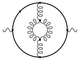
Figure 4: Gluonic double bubble diagrams where the external photon is coupled to a heavy quark and the emitted gluon splits into a gluon loop. The diagrams for the ghost particles which also have to be taken into account, are not depicted.

6. Diagrams with massive quarks and purely gluonic internal lines have been evaluated in [8] through a combination of analytical and numerical methods. The decomposition of the result according to the colour structure will be important for the discussion in Section 5 below. Terms proportional to $C_{F}^{2}$ with a threshold singularity proportional to $(\pi\alpha_{s})^{2}/\beta$ are present in abelian and nonabelian theories as well, whereas terms proportional to $C_{F}C_{A}$ with a logarithmic threshold singularity are characteristic for the nonabelian structure of the theory, with a behaviour similar to the $C_{F}Tn_{\ell}$ term. This leads to the decomposition

$$R_{c}^{(2)}=C_{F}^{2}R_{A}^{(2)}+C_{F}C_{A}R_{NA}^{(2)}+TC_{F}n_{\ell}R_{cq}^{(2)}+TC_{F}R_{cc}^{(2)}+TC_{F}\delta R_{cb}^{(2)}\,,$$ (21)

where $\delta R_{cb}^{(2)}$ is the contribution with an internal $b$ quark loop obtained in analogy to Eq. (4).

The following approximations have been derived in [8]:

$$R_{A}^{(2)} = \frac{(1-\beta^{2})^{4}}{\beta}\,\frac{3\pi^{4}}{8}-12\,\rho^{(1)}+\beta\,\frac{2619}{64}-\beta^{3}\,\frac{2061}{64}+\frac{81}{8}\left(1-\beta^{2}\right)\ln p$$ (22)

$$-198\left(\frac{M_{c}^{2}}{s}\right)^{3/2}\left(\beta^{4}-2\beta^{2}\right)^{6}$$

$$+100\,p^{3/2}(1-p)\left(2.08-1.57\,p+0.405\,p^{2}\right)\,,$$

$$R_{NA}^{(2)} = R_{g}^{(2)}\Big{|}_{\xi=4}+\beta\,\frac{351}{32}-\beta^{3}\,\frac{297}{32}$$ (23)

$$-18\left(\frac{M_{c}^{2}}{s}\right)^{3/2}\left(\beta^{4}-2\beta^{2}\right)^{4}$$

$$+50\,p^{3/2}(1-p)\left(1.41-1.24\,p+0.96\,p^{2}\right)\,,$$

where $p=(1-\beta)/(1+\beta)$. $R_{g}^{(2)}|_{\xi=4}$ is the contribution from gluonic double bubble diagrams (see Fig. 4) for the special choice of the gauge parameter $\xi=4$ and reads [15]

$$R_{g}^{(2)}\Big{|}_{\xi=4}=\left(\frac{11}{4}\ln\frac{\mu^{2}}{4s}+\frac{31}{12}\right)\rho^{(1)}-\frac{33}{4}\,\delta^{(2)}\,,$$ (24)

with $\rho^{(1)}$ and $\delta^{(2)}$ given in Eqs. (8) and (19), respectively. The first lines of Eqs. (22) and (23) consist of the exactly known high energy and threshold contributions, the second and third lines represent a numerically small reminder.

3 Cross section for the heavy quark production

Figure 5: The functions $R_{c}$, $R_{b}$ and $R_{t}$ in NLO plus dominant NNLO terms versus $\sqrt{s}$ for three different scales, $\mu^{2}=M_{Q}^{2}$ (dashed), $\mu^{2}=(2M_{Q})^{2}$ (solid) and $\mu^{2}=s$ (dotted curves). For comparison, also shown are the Born (wide dots) and ${\cal O}(\alpha_{s})$ results ($\mu^{2}=(2M_{Q})^{2}$, dash-dotted).

The collection of the results presented in the previous section provides all tools necessary for a complete description of the cross section in NLO, including charm, bottom and top mass terms. This allows for the prediction of the charm, bottom and top cross sections in the regions where quark masses cannot be neglected but where the resummation of Coulomb terms, characteristic for the regime very close to threshold, is not yet necessary, see the discussion below. As stated above, the terms proportional to $Q_{c}^{2}$ and $\sum_{i=u,d,s}Q_{i}^{2}$ are invariant under renormalization group transformations separately, and only terms proportional to $Q_{c}^{2}$ will be considered in the following. Mutatis mutandis the same formulae are applicable to bottom quark production. For top quarks only the piece induced by the electromagnetic current will be considered, the axial part has been calculated in [16, 14, 17].

Fixed order perturbation theory is inapplicable very close to the production threshold, in the region where $\alpha_{s}/\beta$ is of order one or larger. In this region terms proportional to $(\alpha_{s}/\beta)^{n}$ have to be resummed. However, it will be demonstrated in Section 5 that the first three terms in the perturbative expansion provide a good description down to fairly small values of $\beta$. Specifically, the relative deviation amounts to 0.9/1.7/3.3% for $C_{F}\pi\alpha_{s}/\beta=2/2.5/\pi$, respectively. These values lie well within the radius of convergence $C_{F}\pi\alpha_{s}/\beta<2\pi$ of the resummed series. Taking the requirement $C_{F}\pi\alpha_{s}/\beta<2$ as a guiding principle and incorporating the running of the coupling constant one would admit the strictly perturbative, fixed order treatment down to energy values which are 1 GeV above the nominal threshold for bottom quarks and even less for charm quarks. However, since the perturbative treatment can only be applied beyond the highest $c\bar{c}$ and $b\bar{b}$ bound states, we take 5 GeV for charm and 11.5 GeV for bottom quarks as lowest center of mass energy values. For top, on the other hand, the limit $C_{F}\pi\alpha_{s}/\beta<2$ corresponds to energies about $12$ GeV above $2M_{t}$.

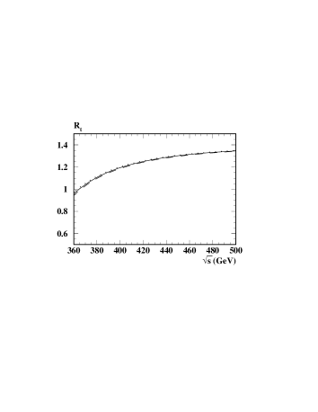
(a)	(b)

Figure 6: Variation of $\alpha_{s}^{(5)}(M_{Z}^{2})$ (a) and the quark masses (b). In (a) the solid, dashed and dotted curves correspond to $\alpha_{s}^{(5)}(M_{Z}^{2})=0.118,0.115$ and $0.121$, respectively. In Figs. (b) for the solid curves ($M_{c}$,$M_{b}$,$M_{t}$)=$(1.6,4.7,175)$ GeV is chosen. The dashed curves correspond to the upper ($(1.8,5.0,180)$ GeV) and the dotted curves to the lower limits ($(1.4,4.4,170)$ GeV). The scale $\mu^{2}=(2M_{Q})^{2}$ has been adopted.

Figure 7: $R(s)$ plotted against $\sqrt{s}$. The scale $\mu^{2}=s$ has been adopted. The dashed curves correspond to the values $M_{c}=1.8$ GeV, $M_{b}=5.0$ GeV and $\alpha_{s}(M_{Z}^{2})=0.121$, whereas for the solid curves $M_{c}=1.4$ GeV, $M_{b}=4.4$ GeV and $\alpha_{s}(M_{Z}^{2})=0.115$ is used. The dotted lines show a recent compilation of the available experimental data. The central curves correspond to the mean values, upper and lower curves indicate the combined statistical and systematical errors.

The compensation between phase space suppression and Coulomb enhancement leads to a fairly flat energy dependence of $R(s)$ even relatively close to threshold (see Fig. 5). In [4, 5] it has been demonstrated for ${\cal O}(\alpha_{s})$ and ${\cal O}(\alpha_{s}^{2})$, respectively, that this behaviour is well approximated by the first terms in the large momentum expansion. Assuming that the same line of reasoning is applicable also in order $\alpha_{s}^{3}$, the dominant NNLO corrections can be incorporated [2, 9, 18]:

$$R_{c,ns}^{(3)} = 3\,\Bigg{\{}-6.637+17.296\ln\frac{\mu^{2}}{s}+7.563\ln^{2}\frac{\mu^{2}}{s}$$ (25)

$$\mbox{}+n_{f}\left(-1.200-2.088\ln\frac{\mu^{2}}{s}-0.917\ln^{2}\frac{\mu^{2}}{s}\right)$$

$$\mbox{}+n_{f}^{2}\left(-0.005+0.038\ln\frac{\mu^{2}}{s}+0.028\ln^{2}\frac{\mu^{2}}{s}\right)+\frac{M_{c}^{2}}{s}\Bigg{[}347.168-378.000\ln\frac{\mu^{2}}{M_{c}^{2}}$$

$$\mbox{}-9.000\ln^{2}\frac{\mu^{2}}{M_{c}^{2}}+974.250\ln\frac{\mu^{2}}{s}-114.000\ln\frac{\mu^{2}}{M_{c}^{2}}\ln\frac{\mu^{2}}{s}+213.750\ln^{2}\frac{\mu^{2}}{s}$$

$$\mbox{}+n_{f}\left(-67.619+17.333\ln\frac{\mu^{2}}{M_{c}^{2}}+2.000\ln^{2}\frac{\mu^{2}}{M_{c}^{2}}-82.167\ln\frac{\mu^{2}}{s}\right.$$

$$\left.\mbox{}+4.000\ln\frac{\mu^{2}}{M_{c}^{2}}\ln\frac{\mu^{2}}{s}-17.000\ln^{2}\frac{\mu^{2}}{s}\right)$$

$$\mbox{}+n_{f}^{2}\left(1.218+1.444\ln\frac{\mu^{2}}{s}+0.333\ln^{2}\frac{\mu^{2}}{s}\right)\Bigg{]}\Bigg{\}}.$$

Inclusion of these terms will lead to the correct NNLO predictions for larger energies, say above $7$ or $8$ GeV, allowing at the same time for a smooth transition to NLO accuracy for lower energies. The singlet terms proportional to $(\sum Q_{i})^{2}$ are small [2] and have been neglected in Eq. (25). In total one thus finds:

$$R_{c} = Q_{c}^{2}\left(R_{c}^{(0)}+\frac{\alpha_{s}^{(4)}(\mu^{2})}{\pi}C_{F}R_{c}^{(1)}+\left(\frac{\alpha_{s}^{(4)}(\mu^{2})}{\pi}\right)^{2}R_{c}^{(2)}+\left(\frac{\alpha_{s}^{(4)}(\mu^{2})}{\pi}\right)^{3}\,R_{c,ns}^{(3)}\right),$$ (26)

where $R_{c,ns}^{(3)}$ denotes the non-singlet contribution at ${\cal O}(\alpha_{s}^{3})$. In Fig. 5 the predictions are shown for the charm, bottom and top cross sections in the energy regions discussed above. For the value of the coupling $\alpha_{s}^{(5)}(M_{Z}^{2})=0.118$ has been adopted and the on-shell quark masses have been chosen to be $M_{c}=1.6$ GeV, $M_{b}=4.7$ GeV and $M_{t}=175$ GeV. (Note that a complete prediction of the top quark cross section would require the incorporation of the axial contribution.) In order to study the sensitivity of the results to the renormalization scale, $\mu^{2}$ has been chosen as $M_{Q}^{2}$ ($Q=c,b,t$; dashed curves), $4M_{Q}^{2}$ (solid curves) and $s$ (dotted curves). The results are relatively stable against this variation. This agreement, despite the appearance of large logarithms $\ln s/M_{Q}^{2}$ for $\mu^{2}=M_{Q}^{2}$, is a consequence of the NNLO approximation valid at the high energy end. The largest sensitivity towards the choice of $\mu^{2}$ is observed in the intermediate and low energy region for charm production, where $\alpha_{s}$ is large and the corrections are enhanced by large contributions proportional to $\ln\beta$ and $1/\beta$. For comparison $R_{c}$, $R_{b}$ and $R_{t}$ are also plotted in the Born (wide dots) and leading order approximation (dash-dotted, $\mu^{2}=(2M_{Q})^{2}$). The cubic corrections in $\alpha_{s}$ are rather small so that we do not show the NLO corrections separately. For the case of the charm and bottom quark the “remainder” of the Coulomb singularity is still visible and both $R_{c}$ and $R_{b}$ raise for $\sqrt{s}\to 5$ GeV and $\sqrt{s}\to 11.5$ GeV, respectively. For the top quark, however, even $10$ GeV above the nominal pair production threshold a singular behaviour is not visible and $R_{t}$ decreases as $\sqrt{s}$ approaches $360$ GeV.

To study the dependence on the input parameters $M_{Q}$ and $\alpha_{s}^{(5)}(M_{Z}^{2})$, we adopt the choice $\mu^{2}=4M_{Q}^{2}$ and vary $\alpha_{s}^{(5)}(M_{Z}^{2})$ within the currently quoted range $\pm 0.03$ (see Fig. 6(a)) and the quark masses in the range as indicated in Fig. 6(b). These changes indicate the present uncertainties. For $R_{c}$ and $R_{b}$ the higher values of the quark masses also lead to larger cross sections — a consequence of the enhanced Coulomb forces for fixed $\sqrt{s}$. For the top quark the phase space effect is still dominant and the cross section for the choice $M_{t}=180$ GeV is smaller than for $M_{t}=170$ GeV.

$\alpha_{s}^{(5)}(M_{Z}^{2})$	$M_{c}$	$\sqrt{s}$	$5$	$6$	$7$	$8$	$9$	$9.98$	$10.52$
	(GeV)	(GeV)
$0.115$	$1.4$	$R_{c}(s)$	$1.505$	$1.467$	$1.447$	$1.434$	$1.426$	$1.420$	$1.418$
$0.115$	$1.4$	$R(s)$	$3.641$	$3.596$	$3.570$	$3.554$	$3.542$	$3.534$	$3.530$
$0.115$	$1.6$	$R_{c}(s)$	$1.538$	$1.486$	$1.459$	$1.443$	$1.432$	$1.425$	$1.422$
$0.115$	$1.6$	$R(s)$	$3.674$	$3.615$	$3.582$	$3.562$	$3.548$	$3.538$	$3.534$
$0.115$	$1.8$	$R_{c}(s)$	$1.575$	$1.507$	$1.473$	$1.452$	$1.439$	$1.431$	$1.427$
$0.115$	$1.8$	$R(s)$	$3.711$	$3.636$	$3.596$	$3.572$	$3.556$	$3.544$	$3.539$
$0.118$	$1.4$	$R_{c}(s)$	$1.516$	$1.473$	$1.451$	$1.438$	$1.430$	$1.424$	$1.421$
$0.118$	$1.4$	$R(s)$	$3.659$	$3.608$	$3.581$	$3.563$	$3.550$	$3.541$	$3.537$
$0.118$	$1.6$	$R_{c}(s)$	$1.553$	$1.494$	$1.465$	$1.447$	$1.436$	$1.429$	$1.425$
$0.118$	$1.6$	$R(s)$	$3.696$	$3.629$	$3.594$	$3.572$	$3.557$	$3.546$	$3.542$
$0.118$	$1.8$	$R_{c}(s)$	$1.598$	$1.519$	$1.480$	$1.458$	$1.444$	$1.434$	$1.430$
$0.118$	$1.8$	$R(s)$	$3.741$	$3.654$	$3.609$	$3.583$	$3.565$	$3.552$	$3.547$
$0.121$	$1.4$	$R_{c}(s)$	$1.527$	$1.480$	$1.456$	$1.442$	$1.433$	$1.427$	$1.424$
$0.121$	$1.4$	$R(s)$	$3.677$	$3.621$	$3.591$	$3.572$	$3.559$	$3.549$	$3.545$
$0.121$	$1.6$	$R_{c}(s)$	$1.569$	$1.503$	$1.471$	$1.452$	$1.440$	$1.432$	$1.429$
$0.121$	$1.6$	$R(s)$	$3.719$	$3.644$	$3.605$	$3.582$	$3.566$	$3.554$	$3.549$
$0.121$	$1.8$	$R_{c}(s)$	$1.622$	$1.531$	$1.488$	$1.463$	$1.448$	$1.438$	$1.434$
$0.121$	$1.8$	$R(s)$	$3.771$	$3.672$	$3.623$	$3.593$	$3.574$	$3.561$	$3.555$

Table 1: Numerical values for $R(s)$ and $R_{c}(s)$. The scale $\mu^{2}=s$ has been chosen. For the evaluation of $R_{c}(s)$ Eq. (26) has been used. $R(s)$ is the proper sum of $R_{uds}(s)$ (Eq. (5)) and $R_{c}(s)$ with $M_{b}=4.7$ GeV.

$\alpha_{s}^{(5)}(M_{Z}^{2})$	$M_{b}$	$\sqrt{s}$	$11.5$	$12$	$13$	$14$	$15$	$40$
	(GeV)	(GeV)
$0.115$	$4.4$	$R_{b}(s)$	$0.372$	$0.371$	$0.368$	$0.366$	$0.364$	$0.349$
$0.115$	$4.4$	$R(s)$	$3.899$	$3.895$	$3.888$	$3.881$	$3.876$	$3.827$
$0.115$	$4.7$	$R_{b}(s)$	$0.372$	$0.371$	$0.369$	$0.367$	$0.365$	$0.349$
$0.115$	$4.7$	$R(s)$	$3.899$	$3.895$	$3.889$	$3.882$	$3.877$	$3.827$
$0.115$	$5.0$	$R_{b}(s)$	$0.370$	$0.370$	$0.369$	$0.368$	$0.366$	$0.350$
$0.115$	$5.0$	$R(s)$	$3.897$	$3.894$	$3.889$	$3.883$	$3.878$	$3.827$
$0.118$	$4.4$	$R_{b}(s)$	$0.376$	$0.374$	$0.371$	$0.368$	$0.365$	$0.350$
$0.118$	$4.4$	$R(s)$	$3.911$	$3.906$	$3.897$	$3.890$	$3.884$	$3.832$
$0.118$	$4.7$	$R_{b}(s)$	$0.377$	$0.375$	$0.372$	$0.370$	$0.367$	$0.350$
$0.118$	$4.7$	$R(s)$	$3.911$	$3.907$	$3.899$	$3.891$	$3.885$	$3.832$
$0.118$	$5.0$	$R_{b}(s)$	$0.377$	$0.376$	$0.373$	$0.371$	$0.368$	$0.350$
$0.118$	$5.0$	$R(s)$	$3.911$	$3.907$	$3.900$	$3.893$	$3.887$	$3.832$
$0.121$	$4.4$	$R_{b}(s)$	$0.381$	$0.378$	$0.374$	$0.370$	$0.367$	$0.350$
$0.121$	$4.4$	$R(s)$	$3.922$	$3.917$	$3.907$	$3.899$	$3.892$	$3.837$
$0.121$	$4.7$	$R_{b}(s)$	$0.383$	$0.380$	$0.376$	$0.372$	$0.369$	$0.350$
$0.121$	$4.7$	$R(s)$	$3.924$	$3.919$	$3.909$	$3.901$	$3.894$	$3.837$
$0.121$	$5.0$	$R_{b}(s)$	$0.384$	$0.382$	$0.377$	$0.374$	$0.371$	$0.351$
$0.121$	$5.0$	$R(s)$	$3.926$	$3.920$	$3.911$	$3.903$	$3.896$	$3.837$

Table 2: Numerical values for $R(s)$ and $R_{b}(s)$. The scale $\mu^{2}=s$ has been chosen. For the evaluation of $R_{b}(s)$ Eq. (26) with obvious modifications has been used. $R(s)$ is the proper sum of $R_{udsc}(s)$ (obtained from Eq. (5)) where in addition charm mass effects of order $M_{c}^{2}/s$ have been included (Eqs. (27) and (28)) and $R_{b}(s)$ ($M_{c}=1.6$ GeV).

$\mu$	$\sqrt{s}$	$5$	$6$	$7$	$8$	$9$	$9.98$	$10.52$
	(GeV)
$M_{c}$	$R_{c}(s)$	$1.514$	$1.437$	$1.409$	$1.400$	$1.397$	$1.398$	$1.399$
$2M_{c}$	$R_{c}(s)$	$1.553$	$1.484$	$1.450$	$1.432$	$1.421$	$1.414$	$1.411$
$\sqrt{s}$	$R_{c}(s)$	$1.553$	$1.494$	$1.465$	$1.447$	$1.436$	$1.429$	$1.425$
$2\sqrt{s}$	$R_{c}(s)$	$1.541$	$1.493$	$1.466$	$1.449$	$1.438$	$1.430$	$1.427$

Table 3: Numerical values for $R_{c}(s)$ for different choices of $\sqrt{s}$ and $\mu$. The values $\alpha_{s}^{(5)}(M_{Z}^{2})=0.118$, $M_{c}=1.6$ GeV and $M_{b}=4.7$ GeV have been chosen.

$\mu$	$\sqrt{s}$	$11.5$	$12$	$13$	$14$	$15$	$40$
	(GeV)
$M_{b}$	$R_{b}(s)$	$0.386$	$0.381$	$0.375$	$0.370$	$0.366$	$0.349$
$2M_{b}$	$R_{b}(s)$	$0.379$	$0.377$	$0.373$	$0.370$	$0.367$	$0.349$
$\sqrt{s}$	$R_{b}(s)$	$0.377$	$0.375$	$0.372$	$0.370$	$0.367$	$0.350$
$2\sqrt{s}$	$R_{b}(s)$	$0.370$	$0.370$	$0.369$	$0.368$	$0.366$	$0.350$

Table 4: Numerical values for $R_{b}(s)$ for different choices of $\sqrt{s}$ and $\mu$. The values $\alpha_{s}^{(5)}(M_{Z}^{2})=0.118$, $M_{c}=1.6$ GeV and $M_{b}=4.7$ GeV have been chosen.

It is now possible to give a prediction for $R(s)$ in the energy range above $\sqrt{s}\approx 2$ GeV with the exception of small windows of $1$ to $2$ GeV above the thresholds for open charm and bottom production, respectively. Below the charm meson threshold at $\sqrt{s}=2M_{D}$ the charm quark is treated as heavy and Eqs. (1) and (4) are used with $n_{\ell}=3$, and with $\alpha_{s}^{(4)}$ and $M_{b}$ replaced by $\alpha_{s}^{(3)}$ and $M_{c}$, respectively. For $5$ GeV$\;\hbox to0.0pt{\lower 3.5pt\hbox{$\mathchar 0\relax\sim$}\hss}\raise 1.0pt\hbox{$<$}\;\sqrt{s}\;\hbox to0.0pt{\lower 3.5pt\hbox{$\mathchar 0\relax\sim$}\hss}\raise 1.0pt\hbox{$<$}\;10.5$ GeV Eqs. (5) and (21) are directly applicable with $n_{f}=n_{\ell}+1=4$. For the case with external charm and internal bottom quark an expression analogue to Eq. (4) is used. Above the bottom threshold the sum over $i$ in Eqs. (1) and (2) includes also the charm contribution and consequently $n_{\ell}=4$ has to be chosen, $\alpha_{s}^{(4)}$ and $M_{c}$ have to be replaced by $\alpha_{s}^{(5)}$ and $M_{b}$. The dominant charm mass terms are included through the leading terms in the $M_{c}^{2}/s$ approximation. The quadratic charm mass corrections of order $\alpha_{s}^{3}$ are given in Eq. (25). The corresponding terms up to order $\alpha_{s}^{2}$ read as follows [19]:

$$\delta R_{M_{c}^{2}}^{(0+1+2)} = 3Q_{c}^{2}\frac{M_{c}^{2}}{s}\Bigg{[}12\frac{\alpha_{s}^{(5)}(\mu^{2})}{\pi}+\left(\frac{\alpha_{s}^{(5)}(\mu^{2})}{\pi}\right)^{2}\left(\frac{189}{2}-24\ln\frac{\mu^{2}}{M_{c}^{2}}-57\ln\frac{s}{\mu^{2}}\right.$$ (27)

$$\mbox{}\left.\qquad\qquad+n_{f}\left(-\frac{13}{3}+2\ln\frac{s}{\mu^{2}}\right)\right)\Bigg{]}.$$

In addition the term

$$3\,\frac{M_{c}^{2}}{s}\,\left(-7.877+0.350n_{f}\right)$$ (28)

which comes from the expansion in $M_{c}^{2}/s$ of diagrams with internal charm loops in $b\bar{b}$ production [9, 18] has to be added to $R_{b,ns}^{(3)}$.

In Fig. 7 $R(s)$ is plotted versus $\sqrt{s}$ for the three energy intervals. Solid and dashed curves show our prediction from perturbative QCD, where the extreme values from the variation of $\alpha_{s}^{(5)}(M_{Z}^{2})$ and the masses are considered and the scale $\mu^{2}=s$ has been adopted. For comparison we also plot a recent compilation of the available experimental data [20] from the inclusive measurements of $R$. The central dotted curves correspond to the mean values, upper and lower dotted curves indicate the combined statistical and systematical errors.

In Tabs. 1 and 2 numerical values are listed for the energy range between the charm and bottom threshold and above the bottom threshold, respectively. For completeness the terms of order $\alpha_{s}^{3}$ to $R_{\rm light}$ are also taken into account. They are obtained from Eq. (25) neglecting the mass corrections with $n_{f}=4$ (Tab. 1) and $n_{f}=5$ (Tab. 2), respectively. In Tabs. 3 and 4 the dependence of $R_{c}$ and $R_{b}$ on the renormalization scale $\mu$ is displayed with $M_{Q}$ and $\alpha_{s}$ fixed to their central values.

It is evident that the uncertainties in the prediction are far below the experimental errors in this “low” energy region. These results could therefore be used to fit the currently available data and to allow for an improved input into the analysis of the running electromagnetic coupling constant $\alpha$.

4 Hadronic vacuum polarization and the running electroweak coupling

One of the important ingredients of electroweak precision tests is the effect of the hadronic vacuum polarization on the running of the electromagnetic coupling. Using a dispersion relation, it is expressed [21] through $R(s)$

$$\Delta\alpha_{\rm had}^{(5)}(M_{Z}^{2}) = -\frac{\alpha M_{Z}^{2}}{3\pi}\,\mbox{Re}\,\int_{4m_{\pi}^{2}}^{\infty}\,{\rm d}s\,\frac{R(s)}{s\left(s-M_{Z}^{2}-i\epsilon\right)}$$ (29)

and contributes together with the well known leptonic contributions to the running of the electromagnetic coupling

$$\alpha(s) = \frac{\alpha(0)}{1-\Delta\alpha^{(5)}_{\rm had}(s)-\Delta\alpha_{\rm lep}(s)},$$ (30)

where $\alpha(0)=1/137.0359895$ is the fine structure constant. Top quark contributions are not considered in this context. Also QED corrections are not included as they are of the order of a few per mill only.

$\alpha_{s}^{(5)}(M_{Z}^{2})$	$0.115$			$0.118$			$0.121$
Energy range
$2.00-2.50$ GeV	7.54			7.58			7.62
$2.50-3.00$ GeV	6.12			6.15			6.18
$3.00-3.73$ GeV	7.27			7.30			7.33
$M_{c}$ (GeV)	$1.4$	$1.6$	$1.8$	$1.4$	$1.6$	$1.8$	$1.4$	$1.6$	$1.8$
Energy range
$3.73-5.00$ GeV	9.73	9.74	9.74	9.77	9.77	9.77	9.80	9.80	9.80
(without $c\bar{c}$)
$5.00-5.50$ GeV	5.37	5.41	5.46	5.40	5.44	5.50	5.42	5.47	5.54
$5.50-6.00$ GeV	4.88	4.91	4.94	4.89	4.93	4.97	4.91	4.95	4.99
$6.00-9.46$ GeV	25.30	25.37	25.46	25.37	25.45	25.55	25.44	25.53	25.63
$9.46-10.52$ GeV	5.88	5.89	5.90	5.90	5.90	5.91	5.91	5.92	5.93
$5.50-10.52$ GeV	36.06	36.17	36.30	36.16	36.28	36.43	36.26	36.39	36.55
$M_{b}$ (GeV)	$4.4$	$4.7$	$5.0$	$4.4$	$4.7$	$5.0$	$4.4$	$4.7$	$5.0$
Energy range
$10.52-11.50$ GeV	4.94	4.94	4.95	4.95	4.95	4.96	4.96	4.96	4.97
(without $b\bar{b}$)
$11.50-12.00$ GeV	2.61	2.61	2.61	2.62	2.62	2.62	2.63	2.63	2.63
$12.00-12.50$ GeV	2.51	2.51	2.51	2.51	2.51	2.51	2.52	2.52	2.52
$12.50-13.00$ GeV	2.41	2.41	2.41	2.42	2.42	2.42	2.42	2.42	2.42
$13.00-40.00$ GeV	72.78	72.80	72.81	72.90	72.92	72.94	73.03	73.04	73.06
$40.00-\infty$ GeV	42.61	42.61	42.62	42.67	42.67	42.67	42.73	42.73	42.73
$12.00-\infty$ GeV	120.31	120.33	120.34	120.50	120.52	120.54	120.70	120.72	120.74

Table 5: Contributions to $\Delta\alpha^{(5)}_{\rm had}(M_{Z}^{2})\times 10^{4}$ for different energy regions, quark masses and $\alpha_{s}^{(5)}(M_{Z}^{2})$. The scale $\mu^{2}=s$ has been adopted. Below the charm threshold the value $M_{c}=1.6$ GeV is chosen. In the energy ranges $3.73-5.00$ GeV and $10.52-11.50$ GeV for $R(s)$ the formulae valid below the corresponding quark threshold have been used.

$\mu$	$M_{c}$	$2M_{c}$	$\sqrt{s}$	$2\sqrt{s}$
Energy range
$5.00-5.50$ GeV	5.37	5.44	5.44	5.43
$5.50-6.00$ GeV	4.85	4.92	4.93	4.92
$6.00-9.46$ GeV	25.10	25.35	25.45	25.46
$9.46-10.52$ GeV	5.85	5.88	5.90	5.91
$5.50-10.52$ GeV	35.80	36.14	36.28	36.28
$\mu$	$M_{b}$	$2M_{b}$	$\sqrt{s}$	$2\sqrt{s}$
Energy range
$11.50-12.00$ GeV	2.62	2.62	2.62	2.62
$12.00-12.50$ GeV	2.52	2.51	2.51	2.51
$12.50-13.00$ GeV	2.42	2.42	2.42	2.41
$13.00-40.00$ GeV	72.89	72.91	72.92	72.92
$40.00-\infty$ GeV	42.63	42.65	42.67	42.67
$12.00-\infty$ GeV	120.45	120.49	120.52	120.52

Table 6: Contribution to $\Delta\alpha^{(5)}_{\rm had}(M_{Z}^{2})\times 10^{4}$ for different energy regions and different choices of $\mu$ for the most heavy quark contribution (for the remaining light quarks the scale $\mu^{2}=s$ has been adopted). The values $\alpha_{s}^{(5)}(M_{Z}^{2})=0.118$, $M_{c}=1.6$ GeV and $M_{b}=4.7$ GeV have been chosen.

Energy range	this work	Ref. [22]
$5.00-9.46$ GeV	$(35.32-35.81)\pm 0.4$	$32.63$
$12.00-40.00$ GeV	$(77.82-77.84)\pm 0.2$	$79.22$

Table 7: Comparison of $\Delta\alpha^{(5)}_{\rm had}(M_{Z}^{2})\times 10^{4}$ evaluated in this work with the data analyzed in [22]. The scale $\mu^{2}=s$ has been chosen for the respective light quark contributions and varied in the range between $M_{Q}^{2}$ and $s$ for the most heavy quark. The errors arise from the variation of $M_{c}$, $M_{b}$ and $\alpha_{s}^{(5)}(M_{Z}^{2})$ (see Tab. 5).

The detailed phenomenological analyses in Refs. [22, 23] have made use of the full set of data obtained by many different experiments for energies from just above the two pion threshold up to $40$ GeV. Although different prescriptions for the interpolation have been used in the different papers, the most recent results are in fair agreement. In the high energy region (typically above $40$ GeV [22]) the prediction for $R(s)$ based on perturbative QCD with massless quarks has been employed. A significant part of the final error originates from the region where perturbation theory should be reasonably valid: the light quark continuum, say above $2$ GeV, the continuum above the charmonium resonances and below the bottom threshold and the region between 12 and 40 GeV, i.e. above the Upsilon resonances. In view of the results presented in the previous chapters one may employ perturbative QCD also in these regions. This might lead to a reduction of the error, albeit at the price of a more pronounced dependence on perturbative QCD. (For early studies along this line see also [22, 23].)

In Tab. 5 and 6 the contributions to $\Delta\alpha^{(5)}_{\rm had}$ are displayed for a variety of input parameters and renormalization scales. Since the validity of our perturbative treatment is more doubtful just above the respective charm and bottom thresholds, the contributions from a variety of intervals are displayed separately. Once improved data are available, these theoretical numbers could be replaced by more precise experimental ones. In Tab. 7 our results are compared to the analysis of [22] for two energy ranges. For the lower energy interval from $5.00-9.46$ GeV our QCD prediction for $\Delta\alpha^{(5)}_{\rm had}$ is bigger than the value obtained by including experimental data by about 9%. In contrast, for the energy interval from $12-40$ GeV, perturbative QCD gives a value slightly smaller than the one obtained from integrating the experimental $R(s)$ values. This behaviour is already clear from Fig. 7, where we indicate the range of experimental data in comparison to $R(s)$ from perturbative QCD.

If one subtracts the narrow Upsilon resonances, QCD can be applied even up to the threshold for $B$ meson production. In fact, recent experimental investigations at 10.52 GeV [24] are nicely consistent with perturbative QCD. The additional contributions from the continuum cross section in the intervals between $3.73$ GeV and $5.00$ GeV (without $c\bar{c}$) and between $9.46$ GeV and $10.52$ GeV (without $b\bar{b}$) are also listed in Tab. 5. For the perturbative contributions through the range from $\sqrt{s}=3$ GeV to $\infty$ without charmonium and open charm contributions below $5$ GeV and $\Upsilon$ and open bottom contributions below 11.5 GeV one finds

$$\Delta\alpha^{(5)}_{\rm had}|_{\rm pert} = \left[(186.27-186.87)\pm 0.70\right]\times 10^{-4}$$ (31)

where the range is due to the variation of $\mu$ for the heavy quark contribution and the error due to uncertainties in the parameters. A more detailed discussion of the impact of these calculations will be given elsewhere.

5 The region for small $\beta$ – closer to the threshold

In the high energy limit, say down to $s\approx 8M_{Q}^{2}$, the cross section in ${\cal O}(\alpha_{s})$ and ${\cal O}(\alpha_{s}^{2})$ is well described by the massless approximation plus the leading terms of the expansion in $M_{Q}^{2}/s$ up to $(M_{Q}^{2}/s)^{6}$ [25, 5]. The bulk of the large logarithms is resummed by taking $\,\mu^{2}=s\,$ for the renormalization scale and adopting the $\overline{\rm MS}$ definition of the running mass. The fixed order result as given above is evidently adequate in the intermediate energy region, with the requirement that $C_{F}\pi\alpha_{s}/\beta$ is not yet too large, i.e. safely away from the threshold regime, where the conventional multi-loop expansion breaks down. Otherwise some care has to be taken to control the higher order terms proportional to $(C_{F}\pi\alpha/\beta)^{n}$ with $n\geq 0$. As far as dominant and subdominant contributions of this sort are concerned, their structure is understood from nonrelativistic considerations and will be briefly outlined in the following for the case $C_{F}\pi\alpha_{s}\;\hbox to0.0pt{\lower 3.5pt\hbox{$\mathchar 0\relax\sim$}\hss}\raise 1.0pt\hbox{$<$}\;\beta\ll 1$.

Let us in a first step discuss those terms which are multiplied by the colour factor $C_{F}$ only and which are relevant for QCD and QED. For the dominant contributions to the cross section in the nonrelativistic limit, often called “Sommerfeld factor” in literature, the leading terms in an expansion in $x_{S}=C_{F}\pi\alpha_{s}/\beta$ are given by

$$R^{\rm thr} = 3Q_{Q}^{2}\frac{3}{2}\frac{\beta x_{S}}{1-e^{-x_{S}}}$$ (32)

$$= 3Q_{Q}^{2}\frac{3}{2}\,\beta\left(1+\frac{x_{S}}{2}+\frac{B_{1}x_{S}^{2}}{2!}-\frac{B_{2}x_{S}^{4}}{4!}+\frac{B_{3}x_{S}^{6}}{6!}-\ldots+(-1)^{(n+1)}\frac{B_{n}x_{S}^{2n}}{(2n)!}\pm\ldots\right)$$

$$= 3Q_{Q}^{2}\frac{3}{2}\,\beta\left(1+C_{F}\frac{\alpha_{s}}{\pi}\frac{\pi^{2}}{2\beta}+C_{F}^{2}\left(\frac{\alpha_{s}}{\pi}\right)^{2}\frac{\pi^{4}}{12\beta^{2}}+\ldots\right),$$

where $B_{n}$ are the Bernoulli numbers: $B_{1}=1/6,\,B_{2}=1/30,\,B_{3}=1/42,\,\ldots\,\,\,$. It should be noted that the Sommerfeld factor is entirely of long-distance origin and proportional to the imaginary part of the nonrelativistic Green function for the Coulomb potential [26], i.e. governed by the continuum Coulomb wave function. These terms are predicted from a consideration, where the $Q\bar{Q}$ production process is decomposed into a short distance part (to be eventually corrected by short distance QCD corrections) and a long distance part, which is governed by the Coulomb wave function, in other words, by the imaginary part of the nonrelativistic Green function for the Coulomb potential [27, 28].

Resummed and fixed order results have to coincide in the region of small $x_{S}$. Thus it is instructive to compare the Sommerfeld factor and the sum of the first three terms in the expansion (32) (corresponding to Born, one- and two-loop contributions, respectively) for various values of $x_{S}$ which are not too much larger than one. It is remarkable that the sum of the first three terms in Eq. (32) provides an excellent approximation not only for small values of $x_{S}$, but even up to $x_{S}=2$ with a relative deviation of less than 1%. Even for $x_{S}=\pi$, corresponding to $C_{F}\alpha_{s}/\beta=1$, the deviation amounts to 3.3% only.

In addition, based on the consideration that the cross section for nonrelativistic energies can be decomposed into long- and short-distance contributions one obtains in QED an additional correction factor which comes from relativistic momenta involved in the transverse photon exchange. This factor, which is quite familiar from the single-photon annihilation contributions to the positronium hyperfine splitting [29] and from the corrections to quarkonium annihilation through a virtual photon [30], can be derived from the threshold behaviour of the one-loop corrections [13]. In combination one thus anticipates the following behaviour

$$R^{\rm thr}=3Q_{Q}^{2}\beta\,\frac{3-\beta^{2}}{2}\Bigg{[}1+\frac{1}{2}\,C_{F}\frac{\alpha_{s}\pi}{\beta}\,\left(1+\beta^{2}\right)+\frac{1}{12}\left(C_{F}\frac{\alpha_{s}\pi}{\beta}\,\left(1+\beta^{2}\right)\right)^{2}\Bigg{]}\left(1-4C_{F}\,\frac{\alpha_{s}}{\pi}\right)\,.$$ (33)

The inclusion of the subleading $\beta^{2}$ terms in the combinations $(3-\beta^{2})$ and $(1+\beta^{2})/\beta$ is suggested from the structure of Eq. (8) for small $\beta$. An explicit proof for this structure at the NLO level can be found in [31]. Their interpretation as long distance contributions is furthermore motivated by the appearance of the logarithmic terms with the same structure in the $C_{F}Tn_{\ell}$ contributions listed below (see [15] and Eq. (40) of [8]). Even the impact of the running of the coupling constant can be included in this nonrelativistic line of reasoning. In QCD the running of $\alpha_{s}$ is induced by terms proportional to $T\,n_{\ell}$ and $C_{A}$.

For a prediction of the hadronic cross section very close to threshold, i.e. in the regime $\beta\leq C_{F}\pi\alpha_{s}$, the factorization into short- and long-distance contributions analogous to Eq. (33) is desirable, incorporating also the new information from the NLO calculation. Such an analysis requires the resummation of long-distance contributions to all orders and shall not be carried out here. However, the leading terms of the perturbative series for small $\beta$ provide the basis for such a resummation and will be collected in the following.

Let us now recapitulate the threshold behaviour of the various ingredients for $R_{c}$:

$$R_{c}^{(0)} = 3Q_{c}^{2}\,\beta\frac{3-\beta^{2}}{2},$$ (34)

$$R_{c}^{(1)} = R^{(0)}\left[\frac{\pi^{2}(1+\beta^{2})}{2\beta}-4\right]+\ldots\,\,,$$ (35)

$$R_{A}^{(2)} = R^{(0)}\left[\frac{1}{12}\left(\frac{\pi^{2}(1+\beta^{2})}{\beta}\right)^{2}-2\frac{\pi^{2}(1+\beta^{2})}{\beta}\right.$$ (36)

$$\left.\quad\mbox{}-\frac{2}{3}\pi^{2}\left(\ln\frac{\beta}{4}+\frac{35}{12}\right)+\frac{39}{4}-\zeta(3)\right]+\ldots\,\,,$$

$$R_{NA}^{(2)} = R^{(0)}\left[\frac{\pi^{2}(1+\beta^{2})}{\beta}\left(-\frac{11}{24}\ln\frac{4\beta^{2}M_{c}^{2}}{\mu^{2}}+\frac{31}{72}\right)-\frac{11}{3}\ln\frac{\mu^{2}}{M_{c}^{2}}+c\right]+\ldots\,\,,$$ (37)

$$R_{cq}^{(2)} = R^{(0)}\left[\frac{\pi^{2}(1+\beta^{2})}{\beta}\left(\frac{1}{6}\ln\frac{4\beta^{2}M_{c}^{2}}{\mu^{2}}-\frac{5}{18}\right)+\frac{4}{3}\ln\frac{\mu^{2}}{M_{c}^{2}}+\frac{11}{9}\right]+\ldots\,\,,$$ (38)

$$R_{cc}^{(2)} = R^{(0)}\left[\frac{\pi^{2}}{6\beta}\ln\frac{M_{c}^{2}}{\mu^{2}}-\frac{4}{3}\ln\frac{M_{c}^{2}}{\mu^{2}}+\frac{44}{9}-\frac{8}{3}\zeta(2)\right]+\ldots\,\,.$$ (39)

Terms of order $\beta^{2}$ (modulo $\ln\beta$) are neglected. The order $\beta$ terms in Eq. (36) is taken from [32]. Subleading terms in Eq. (37), symbolized by $c$, have not been calculated yet analytically. Assuming a linear dependence on $\beta$, an estimate for the constant $c$ can be extracted from the numerical analysis in [8]. Considering the expansion of $11$ different Padé approximations which show a quite stable behaviour near threshold one obtains

$$c = 24\pm 5\,,$$ (40)

where the error is estimated by taking into account the variation of the predictions for the constant $c$ from the different Padé approximations. This numerical result for $c$ is fairly large, in particular when compared to the corresponding constant $11/9$ in the $C_{F}Tn_{\ell}$ term, Eq. (38).

In total one thus gets:

$$R_{c} = Q_{c}^{2}\Bigg{[}R_{c}^{(0)}+\frac{\alpha_{s}^{(4)}(\mu^{2})}{\pi}C_{F}R^{(1)}$$ (41)

$$+\left(\frac{\alpha_{s}^{(4)}(\mu^{2})}{\pi}\right)^{2}\left(C_{F}^{2}R_{A}^{(2)}+C_{F}C_{A}R_{NA}^{(2)}+TC_{F}n_{\ell}R_{cq}^{(2)}+TC_{F}R_{cc}^{(2)}\right)\Bigg{]}.$$

The renormalization group invariance of this result is apparent: the $\mu$ dependence of $R_{NA}$, $R_{cq}$, and $R_{cc}$ properly compensates the $\mu$ dependence of the ${\cal O}(\alpha_{s})$ term. As stated above, the energies considered in this section will be of order $M_{c}$, implying that $\ln(s/M_{c}^{2})$ is not a large quantity. The transition from $\alpha_{s}^{(n_{f})}$ to $\alpha_{s}^{(n_{\ell})}$ is thus legitimate and easily achieved by absorbing the last term of Eq. (11) in the order $\alpha_{s}$ expression.

The logarithmic singularities and the constants in $R_{NA}$ and $R_{cq}$ which are leading in $\beta$ can be absorbed in the terms of order $\alpha_{s}$ if the $\overline{\rm MS}$ coupling constant is replaced by the coupling governing the potential [33]

$$V_{QCD}(\vec{q}\,^{2}) = -4\pi C_{F}\frac{\alpha_{V}(\vec{q}\,^{2})}{\vec{q}\,^{2}},$$ (42)

$$\alpha_{V}(\vec{q}\,^{2}) = \alpha_{s}^{(n_{\ell})}(\mu^{2})\Bigg{[}1+\frac{\alpha_{s}^{(n_{\ell})}(\mu^{2})}{4\pi}\left(\left(\frac{11}{3}C_{A}-\frac{4}{3}Tn_{\ell}\right)\left(-\ln\frac{\vec{q}\,^{2}}{\mu^{2}}+\frac{5}{3}\right)-\frac{8}{3}C_{A}\right)\Bigg{]},$$

with $\vec{q}\,^{2}=\beta^{2}s$. This is apparent once the sum of the Born cross section plus higher order corrections is rewritten as follows (with $x_{V}=C_{F}\pi\alpha_{V}(\beta^{2}s)\,(1+\beta^{2})/\beta$):

$$R_{c} = Q_{c}^{2}\,R_{c}^{(0)}\Bigg{\{}1+\frac{x_{V}}{2}-4C_{F}\frac{\alpha_{s}^{(3)}(\mu^{2})}{\pi}+\frac{x_{V}^{2}}{12}-4C_{F}\frac{x_{V}}{2}\frac{\alpha_{s}^{(3)}(\mu^{2})}{\pi}$$ (43)

$$+\left(\frac{\alpha_{s}^{(3)}(\mu^{2})}{\pi}\right)^{2}\Bigg{[}C_{F}^{2}\left(-\frac{2}{3}\pi^{2}\left(\ln\frac{\beta}{4}+\frac{35}{12}\right)+\frac{39}{4}-\zeta(3)\right)$$

$$\mbox{}+C_{A}C_{F}\left(-\frac{11}{3}\ln\frac{\mu^{2}}{M_{c}^{2}}+c\right)+C_{F}Tn_{\ell}\left(\frac{4}{3}\ln\frac{\mu^{2}}{M_{c}^{2}}+\frac{11}{9}\right)$$

$$\mbox{}+C_{F}T\left(\frac{44}{9}-\frac{8}{3}\zeta(2)\right)\Bigg{]}\Bigg{\}}+\ldots\,\,.$$

In the transition from Eq. (41) to (43) we have freely dropped terms of order $\alpha_{s}^{3}$. It is evident that the scale in the correction term from hard transverse gluon exchange proportional to $4C_{F}\alpha_{s}^{(3)}(\mu^{2})/\pi$ is of order $M_{c}$, with $\mu_{BLM}=e^{-11/24}M_{c}=0.63M_{c}$ suggested by the BLM prescription [34]. However, as noted before, the corresponding constant $c\approx 24$ in the non-abelian term is markedly different from what would be expected from the BLM procedure.

As stated above these results are strictly applicable in the limit $\pi C_{F}\alpha_{s}\;\hbox to0.0pt{\lower 3.5pt\hbox{$\mathchar 0\relax\sim$}\hss}\raise 1.0pt\hbox{$<$}\;\beta\ll 1$ only. Nevertheless, Eq. (43) provides an important input for the determination of the cross section very close to threshold and even for bound state energies, i.e. for $|\beta|<C_{F}\pi\alpha_{s}$, because it contains all ${\cal O}(\alpha_{s}^{2})$ short-distance effects relevant for the nonrelativistic regime. These short-distance effects, which are specific for the single-photon annihilation process involving massive quark-antiquark pairs, are universal for $|\beta|\ll 1$ regardless whether $|\beta|$ is smaller or larger than $C_{F}\pi\alpha_{s}$. In this respect Eq. (43) even provides an important result for the investigation of leptonic decay widths of the $\Psi$ and the $\Upsilon$ families, and for QCD sum rules for the $b\bar{b}$ system. A discussion of the latter subjects, however, is beyond the scope of this paper.

6 Summary and Conclusions

Predictions for the cross section of massive quark production in $e^{+}e^{-}$ annihilation are presented which are accurate to order $\alpha_{s}^{2}$. Their range of validity extends from high energies down close to threshold, i.e. to center of mass energies of about 5 GeV, 11.5 GeV and $2M_{t}+12$ GeV for charm, bottom and top respectively. Inclusion of the leading and subleading terms of order $\alpha_{s}^{3}$ proportional to $M_{Q}^{2}/s$ allows to connect smoothly the NNLO prediction at high energies with the NLO prediction in the intermediate and “low” energy range. The NLO corrections are sizable and must be taken into account to achieve a prediction with an accuracy better than 10%. The stability of the prediction against variations of the renormalization scale and of the input values for the quark masses and $\alpha_{s}$ has been tested. Even fairly extreme assumptions about the renormalization scale lead to moderate variations in the case of charm and to negligible variations for the heavier quarks. The same holds true for the dependence on the input parameters, the quark masses and the strong coupling constant. Only a change in the charm quark mass has a clearly visible effect on the cross section. Within the large experimental errors, theoretical and experimental results are well consistent. The theoretical results can now be used to perform an universal fit to the data, including the lower energy regions. In view of the sparse data with large errors in the region from $2-3.73$ GeV, from $5-10.52$ GeV and from $11.5-40$ GeV one could also consider to use the predictions based on perturbative QCD to arrive at a more precise value for the running QED coupling at the $Z$ boson mass. A significant reduction of the uncertainty could be obtained.

Acknowledgments

We thank John Outhwaite for providing us with his compilation of the experimental data for the inclusive $R$ measurements. T. Teubner thanks the British PPARC and the University of Durham, where part of this work was carried out. K.G. Chetyrkin appreciates the warm hospitality of the Theoretical group of the Max Planck Institute in Munich where part of this work has been made. A.H. Hoang is supported in part by U.S. Department of Energy under Contract No. DOE DE-FG03-90ER40546.

References

-
[1]
K.G. Chetyrkin, A.L. Kataev and F.V. Tkachov,
Phys. Lett. B 85 (1979) 277;
M. Dine and J. Sapirstein, Phys. Rev. Lett. 43 (1979) 668;
W. Celmaster and R.J. Gonsalves, Phys. Rev. Lett. 44 (1980) 560. -
[2]
S.G. Gorishny, A.L. Kataev and S.A. Larin,
Phys. Lett. B 259 (1991) 144;
L.R. Surguladze and M.A. Samuel, Phys. Rev. Lett. 66 (1991) 560; (E) ibid., 2416;
K.G. Chetyrkin, Phys. Lett. B 391 (1997) 402. - [3] K.G. Chetyrkin, J.H. Kühn and A. Kwiatkowski, Phys. Rep. 277 (1996) 189.
- [4] K.G. Chetyrkin and J.H. Kühn, Nucl. Phys. B 432 (1994) 337.
- [5] K.G. Chetyrkin, R. Harlander, J.H. Kühn and M. Steinhauser, Nucl. Phys. B 503 (1997) 339.
- [6] A.H. Hoang, M. Jeżabek, J.H. Kühn and T. Teubner, Phys. Lett. B 338 (1994) 330.
- [7] A.H. Hoang, J.H. Kühn and T. Teubner, Nucl. Phys. B 452 (1995) 173.
- [8] K.G. Chetyrkin, J.H. Kühn and M. Steinhauser, Phys. Lett. B 371 (1996) 93; Nucl. Phys. B 482 (1996) 213.
- [9] K.G. Chetyrkin and J.H. Kühn, Phys. Lett. B 248 (1990) 359.
- [10] B.A. Kniehl, Phys. Lett. B 237 (1990) 127.
- [11] K.G. Chetyrkin, Phys. Lett. B 307 (1993) 169.
- [12] D.E. Soper and L.R. Surguladze, Phys. Rev. Lett. 73 (1994) 2958.
-
[13]
G. Källén and A. Sabry, K. Dan. Vidensk. Selsk. Mat.-Fys. Medd.
29 (1955) No. 17;
see also: J. Schwinger, Particles, Sources and Fields, Vol. II, (Addison-Wesley, New York, 1973). - [14] A.H. Hoang and T. Teubner, Report Nos. DTP/97/68, UCSD/PHT 97-16 and hep-ph/9707496.
- [15] K.G. Chetyrkin, A.H. Hoang, J.H. Kühn, M. Steinhauser and T. Teubner, Phys. Lett. B 384 (1996) 233.
- [16] K.G. Chetyrkin, J.H. Kühn and M. Steinhauser, Report Nos. MPI/PhT/97-029, TTP97-19 and hep-ph/9705254 (Nucl. Phys. B, in press).
- [17] R. Harlander and M. Steinhauser, Report Nos. MPI/PhT/97-66, TTP97-40 and hep-ph/9710413.
- [18] K.G. Chetyrkin and J.H. Kühn, Phys. Lett. B 406 (1997) 102.
- [19] S.G. Gorishny, A.L. Kataev and S.A. Larin, Nuovo Cim. A 92 (1986) 119.
- [20] J. Outhwaite, private communication.
- [21] N. Cabbibo and R. Gatto, Phys. Rev. 124 (1961) 1577.
- [22] S. Eidelman and F. Jegerlehner, Z. Phys. C 67 (1995) 585.
-
[23]
A.D. Martin and D. Zeppenfeld Phys. Lett. B 345 (1995) 558;
H. Burkhardt and B. Pietrzyk, Phys. Lett. B 356 (1995) 389;
M.L. Swartz, Phys. Rev. D 53 (1996) 5268;
R. Alemany, M. Davier and A. Höcker, Report Nos. LAL-97-02 and hep-ph/9703220. - [24] CLEO Collaboration (R. Ammar et al.), Report Nos. CLNS-97-1493 and hep-ex/9707018.
- [25] K.G. Chetyrkin and J.H. Kühn, Phys. Lett. B 342 (1995) 356.
- [26] M.A. Braun, Sov. Phys. JETP Lett. 27 (1968) 652, Zh. Eksp. Teor. Fiz. 54 (1968) 1220.
- [27] M.B. Voloshin, Nucl. Phys. B 154 (1979) 365.
- [28] H. Leutwyler, Phys. Lett. B 98 (1981) 447.
- [29] R. Karplus and A. Klein, Phys. Rev. 87 (1952) 848.
- [30] R. Barbieri, R. Gatto, R. Kögerler and Z. Kunszt, Phys. Lett. B 57 (1975) 455.
- [31] A.H. Hoang, Report Nos. UCSD/PTH 97-08 and hep-ph/9703404 (Phys. Rev. D, in press).
- [32] A.H. Hoang, Phys. Rev. D 56 (1997) 5851.
-
[33]
W. Fischler, Nucl. Phys. B 129 (1977) 157;
A. Billoire, Phys. Lett. B 92 (1980) 343. -
[34]
S.J. Brodsky, G.P. Lepage and P.B. Mackenzie,
Phys. Rev. D 28 (1983) 228;
S.J. Brodsky and H.J. Lu, Phys. Rev. D 51 (1995) 3652.