BINP-97-11

ISU-HET-97-5

October 1997

$CP$ Violating Anomalous Couplings at a $500$ GeV $e^{+}e^{-}$ Linear Collider A. A. Likhoded^(a), G. Valencia^(b) and O.P. Yushchenko^(c)
(a) Branch of The Institute for Nuclear Physics,
Protvino, 142284 Russia. E-mail: likhoded@mx.ihep.su

^(b) Department of Physics, Iowa State University, Ames IA 50011
E-mail: valencia@iastate.edu

^(c) Institute for High Energy Physics,
Protvino, 142284 Russia. E-mail: yushchenko@mx.ihep.su

We study the sensitivity of a $500$ GeV $e^{+}e^{-}$ Linear Collider to $CP$ violating anomalous couplings. We find that with 50 fb^-1, and taking only one non-zero coupling at a time, the process $e^{+}e^{-}\rightarrow W^{+}W^{-}$ can be used to place the 95% confidence level bounds $|\tilde{\kappa}_{\gamma}|\leq 0.1$, $|\tilde{\kappa}_{Z}|\leq 0.1$ and $|g_{4}^{Z}|\leq 0.1$ from $CP$ even observables. By studying certain distributions in the process $e^{+}e^{-}\rightarrow\mu^{+}\mu^{-}\nu\overline{\nu}$ one of the bounds can be improved to $|g_{4}^{Z}|\leq 0.06$. This process also allows the construction of a $CP$ odd observable which can be used to place bounds on $CP$ violating new physics. At the 95% confidence level we find $|\tilde{\kappa}_{\gamma}|\leq 0.3$, $|\tilde{\kappa}_{Z}|\leq 0.2$ and a much weaker bound for $|g_{4}^{Z}|$.

1 Introduction

In spite of its remarkable phenomenological success there are several aspects of the standard model that remain unexplained. Two of them are the mechanism of electroweak symmetry breaking and the origin of $CP$ violation. A broad class of models in which the electroweak symmetry is broken dynamically by new strong interactions does not contain any new particles sufficiently light to be produced at a 500 GeV $e^{+}e^{-}$ collider. New particles in these models have masses in the TeV range and only manifest themselves indirectly in experiments at lower energies. In general these models may violate $CP$ and this would also manifest itself indirectly at low energy.

It is convenient to describe the phenomenology of the most important features of this type of new physics in a model independent way. This is accomplished by studying a low energy (below a few TeV) effective Lagrangian that contains only the standard model fields and where the effect of the new physics appears as higher dimension operators. These higher dimension operators modify the couplings of the observed particles, inducing “anomalous couplings” whose phenomenology has been studied in detail [1].

In this paper we study the effect of the lowest dimension operators that violate $CP$ in the gauge-boson self-couplings. In has become standard to parameterize the three gauge boson coupling $WWV$ following the notation of Ref. [2]:

$${\cal L}_{WWV}=g_{WWV}\biggl{(}-g_{4}^{V}W^{+}_{\mu}W^{-}_{\nu}(\partial^{\mu}V^{\nu}+\partial^{\nu}V^{\mu})+{i\over 2}\tilde{\kappa}_{V}\epsilon_{\mu\nu\alpha\beta}W^{+}_{\mu}W^{-}_{\nu}V^{\alpha\beta}\biggr{)}$$ (1)

In writing this equation we have already dropped terms proportional to $\tilde{\lambda}_{V}$ because they are of higher dimension. The overall normalization is $g_{WW\gamma}=-e$ and $g_{WWZ}=-e\cot\theta_{W}$. Electro-magnetic gauge invariance forbids the term $g_{4}^{\gamma}$ so we are left with three new $CP$ violating parameters. One of them, $g_{4}^{Z}$, violates $C$ and conserves $P$; whereas the other two, $\tilde{\kappa}_{\gamma}$ and $\tilde{\kappa}_{Z}$ violate $P$ and conserve $C$.

The next to leading order electroweak chiral Lagrangian [3] contains three $CP$ violating operators whose couplings correspond to the lowest dimension contributions to the parameters in Eq. (1). They are [4]:

$${\cal L}_{CP-odd} = 2\alpha_{12}g{\rm Tr}(T{\cal V}_{\mu}){\rm Tr}({\cal V}_{\nu}W^{\mu\nu})$$ (2)

$$+ {1\over 4}\alpha_{13}gg^{\prime}\epsilon^{\mu\nu\rho\sigma}B_{\mu\nu}{\rm Tr}(TW_{\rho\sigma})$$

$$+ {1\over 8}\alpha_{14}g^{2}\epsilon^{\mu\nu\rho\sigma}{\rm Tr}(TW_{\mu\nu}){\rm Tr}(TW_{\rho\sigma})$$

where we have used the notation of Ref. [4]. The relation between these couplings and those in Eq. (1) is $\tilde{\kappa}_{Z}=e^{2}(\alpha_{13}/c^{2}_{W}-\alpha_{14}/s^{2}_{W})$, $\tilde{\kappa}_{\gamma}=-(e^{2}/s^{2}_{W})(\alpha_{13}+\alpha_{14})$ and $g_{4}^{Z}=-e^{2}/(s^{2}_{W}c^{2}_{W})\alpha_{12}$ [4].

We do not wish to reproduce here all the details of the notation of Ref. [4], it is sufficient to remind the reader that the factor $T$ that appears in all three operators constitutes an explicit breaking of custodial symmetry. This implies that if the new physics violates $CP$ maximally (i.e. without suppressions from dimensionless parameters such as mixing angles), the natural size of the coefficients is that of $(v^{2}/\Lambda^{2})\Delta\rho$. These are the same arguments that give the natural size of the lowest dimension parity violating coupling [5]. With $v\approx 246$ GeV and the scale of new physics $\Lambda$ a few TeV we thus expect $\alpha_{12,13,14}\sim 10^{-4}$ if the symmetry breaking sector has a custodial symmetry to explain the smallness of $\Delta\rho$. In Ref. [4] Appelquist and Wu discuss a specific model in which they estimate that the coefficients $\alpha_{12,13,14}$ are indeed of order $10^{-4}$ and correlated with $\Delta\rho$. On the other hand, if $\Delta\rho$ is small accidentally, naive power counting tells us that these couplings could be at the few percent level, ${\cal O}(v^{2}/\Lambda^{2})$. These numbers will help us calibrate the significance of the constraints that we discuss.

The best indirect bound that exists on any of these couplings is $|\tilde{\kappa}_{\gamma}|<2\times 10^{-4}$, which arises from the neutron e.d.m. [6]. This is a very tight constraint, but it is subject to naturalness assumptions. As usual, it is not a substitute for a direct constraint. Previous studies of $W\gamma$ production at an upgraded Tevatron have concluded that it will be possible to place the constraint $|\tilde{\kappa}_{\gamma}|{~{}\raise 1.49994pt\hbox{$<$}\kern-8.50006pt\lower 3.50006pt\hbox{$\sim$}~{}}0.1$ [7]. This is of the same order as the bound that we find in this study for the 500 GeV $e^{+}e^{-}$ collider, but a precise comparison is not possible without further knowledge of the experimental setups.

There have been previous studies of the $CP$ violating anomalous couplings in the process $e^{+}e^{-}\rightarrow W^{+}W^{-}$ [8], but a detailed numerical analysis of the bounds that one can get at a NLC has not been done. The process $e^{+}e^{-}\rightarrow\nu\overline{\nu}Z$ has also been recently considered [9]. The authors of Ref. [9] find that one could place the bound $g_{4}^{Z}{~{}\raise 1.49994pt\hbox{$<$}\kern-8.50006pt\lower 3.50006pt\hbox{$\sim$}~{}}0.1$ by studying a forward-backward asymmetry with $50~{}{\rm fb}^{-1}$.

2 Bounds from observables in $e^{+}e^{-}\rightarrow W^{+}W^{-}$

We start with the process $e^{+}e^{-}\rightarrow W^{+}W^{-}$ at a center of mass energy of 500 GeV without considering any specific decay channel for the $W$ bosons. At this stage we also ignore the $CP$ violating nature of the couplings $\tilde{\kappa}_{\gamma},~{}\tilde{\kappa}_{Z},~{}g_{4}^{Z}$ and look only at the quadratic effects that they induce in the decay distribution. It is possible to study truly $CP$-violating effects that are linear in the couplings in one of two ways. We could include absorptive phases in the form factors associated with Eq. (1) [2, 4]. If these phases arise from the same sector responsible for the anomalous couplings then they do not introduce additional suppression factors. This can be seen, for example, in the model of Ref. [4]. Alternatively, we could construct a $CP$ odd observable involving the polarization vectors of the $W$ bosons. This is equivalent to studying correlations that involve the momenta of the decay products of the $W$-bosons to a specific channel. We take the second approach in the following section.

In this section we consider the $W$ bosons to be final state particles and take into account the efficiency for $W^{+}W^{-}$ pair reconstruction $\epsilon_{WW}=0.15$ [10] in our numerical simulation. Because we are ignoring, for now, the $CP$ violating nature of the couplings, it is possible to bound them using the same $CP$ even observables that we studied in Ref. [11]. The only difference between the $CP$ violating couplings that we study here, and the $CP$ conserving couplings that we studied in Ref. [11] is that the $CP$ violating couplings always appear quadratically in the $CP$ even distributions used to place the bounds. We use the same assumptions about systematic uncertainties and the same analysis of the differential distribution that we described in detail in Ref. [11]. In particular, we use a systematic error $\sim$1.5%. This number arises from an uncertainty in the luminosity measurement of $\simeq$0.5%, an error in the acceptance $\simeq$1%, an error for background subtraction $\simeq$0.5% and a systematic error in the knowledge of the branching ratio $\simeq$0.5%. From a $\chi^{2}$ analysis of $d\sigma/d\cos\theta$ with 5 bins, we find the 95% confidence level bounds (taking only one non-zero coupling at a time):

$$|\tilde{\kappa}_{\gamma}|\leq 0.1,\;|\tilde{\kappa}_{Z}|\leq 0.1,\;|g_{4}^{Z}|\leq 0.09$$ (3)

The best bounds for this process are obtained using four bins, as discussed in Ref. [11]. However, the bounds we obtain using five bins are indistinguishable from those for four bins. We prefer five bins because this will be the optimal number for $e^{+}e^{-}\rightarrow\mu^{+}\mu^{-}\nu\overline{\nu}$ and using the same number of bins in both cases will facilitate a comparison.

     

Figure 1: Allowed (95% C. L.) region from the $CP$ even angular distribution of $e^{+}e^{-}\rightarrow W^{+}W^{-}$ for: a) $\tilde{\kappa}_{Z}~{}-~{}g_{4}^{Z}$ with $\tilde{\kappa}_{\gamma}=0$; b) $\tilde{\kappa}_{\gamma}~{}-~{}g_{4}^{Z}$ with $\tilde{\kappa}_{Z}=0$; c) $\tilde{\kappa}_{\gamma}~{}-~{}\tilde{\kappa}_{Z}$ with $g_{4}^{Z}=0$.

In Figure 1 we present the allowed 95% confidence level regions when we take one of the $CP$ violating couplings to be zero. We see that the bounds are indeed similar to those that can be placed at an upgraded Tevatron [7], and of the same order as the bounds that we found for $CP$ conserving anomalous couplings [11]. The fact that we obtain similar bounds for couplings that contribute linearly to the differential cross-section and for couplings that only contribute quadratically, already indicates that this process is not sensitive to the very small values predicted by naive dimensional analysis.

3 Bounds from observables in $e^{+}e^{-}\rightarrow\mu^{+}\mu^{-}\nu\overline{\nu}$

We now wish to consider a specific channel for the decay of the $W$-bosons so that we can construct correlations that could single out $CP$-violating interactions. With this in mind, we need a final state that is easy to identify and that transforms into itself under $CP$. We thus choose to identify the $W$ pairs by their $\mu\nu$ leptonic decays. We calculate the amplitudes for the process $e^{+}e^{-}\to\mu^{+}\mu^{-}\nu\bar{\nu}$ and generate events for the three following subprocesses:

Subprocess I — $$e^{+}e^{-}\to\mu^{+}\mu^{-}\nu_{\mu}\bar{\nu}_{\mu}\>,$$

Subprocess II — $$e^{+}e^{-}\to\mu^{+}\mu^{-}\nu_{e}\bar{\nu}_{e}\;,$$

Subprocess III — $$e^{+}e^{-}\to\mu^{+}\mu^{-}\nu_{\tau}\bar{\nu}_{\tau}\;.$$

These subprocesses include 20, 21 and 11 Feynman diagrams respectively. The last one does not contain anomalous vertices, and constitutes pure background. Sufficient events are generated with our Monte-Carlo to achieve a $1\%$ statistical error in the value of the cross-section.

We first generate events with a cut on the muon scattering angle and on the muon pair invariant mass:

$$170^{o}\leq\theta\leq 10^{o},~{}~{}~{}M_{\mu\mu}\geq 30~{}{\rm GeV}$$ (4)

The angle $\theta$ is the scattering angle between the $\mu^{-}$ and the $e^{-}$ momenta in the $e^{+}e^{-}$ center of mass frame. To study $CP$ odd observables we need to make sure that our cuts are “$CP$ blind”, so the same cut is imposed on the angle between the $\mu^{+}$ and the $e^{+}$ momenta. These cuts are similar to the ones used by the LEP experiments. After imposing these cuts we assume a muon reconstruction efficiency equal to 1.

The total cross-section for the $e^{+}e^{-}\to\mu^{+}\mu^{-}\nu\bar{\nu}$ process with these cuts is 7.65 fb, which results (with an integrated luminosity of 50 fb^-1) in only 382 events. The resulting bounds will be limited by the small statistics so we will have to relax these cuts later on.

We start by placing bounds on the $CP$ violating anomalous couplings using the following observables:

$$\frac{d\sigma}{d\cos\theta}\>,\;\;\frac{d\sigma}{dp_{\mu}}\>,\;\;\frac{d\sigma}{dp_{\mu\times\mu}}\>,$$ (5)

where $\theta$ is again the scattering angle between the $\mu^{-}$ and the $e^{-}$ momenta in the $e^{+}e^{-}$ center of mass frame; $p_{\mu}$ is the muon three-momentum in the same frame, and $p_{\mu\times\mu}$ is proportional to the $T$-odd correlation $\vec{p}_{e}\cdot[\vec{p}_{\mu^{+}}\times\vec{p}_{\mu^{-}}]$. Numerically we work in the $e^{+}e^{-}$ center of mass frame and use:

$$p_{\mu\times\mu}=\frac{4}{s}[\vec{p}_{\mu^{+}}\times\vec{p}_{\mu^{-}}]_{z}\;,$$ (6)

where the index $z$ denotes the component along the beam direction. With this normalization $p_{\mu\times\mu}$ can take values from $-1$ to 1. If the polarization of the final leptons is not observed, and the beams are not polarized, this correlation serves to analyze the $CP$ properties of the interaction [12]. $CP$ even interactions give rise to symmetric distributions (symmetric about the point $p_{\mu\times\mu}=0$) in $p_{\mu\times\mu}$, whereas $CP$ odd interactions give rise to antisymmetric distributions in $p_{\mu\times\mu}$. The antisymmetric distributions in this correlation will arise from interference between standard model amplitudes and the new $CP$-violating physics and will be linear in the new couplings. Notice that the correlation $p_{\mu\times\mu}$ is also odd under parity. This means that we will get terms proportional to $\tilde{\kappa}_{\gamma,Z}$ from interference with the parity even standard model amplitude and a term proportional to $g_{4}^{Z}$ from interference with the parity odd standard model amplitude.

In Figure 2 we show the differential cross-section predicted by the standard model at lowest order, as a function of $\cos\theta$ and $p_{\mu}$, for $\sqrt{s}=500$ GeV. From these figures we see that the events predicted by the standard model are concentrated at small scattering angles and low muon momentum. Similarly we find that the standard model events have a symmetric distribution in $p_{\mu\times\mu}$ (as corresponds to CP conservation) that is very strongly peaked at $p_{\mu\times\mu}=0$.

     

Figure 2: Standard model differential cross-section for the process $e^{+}e^{-}\rightarrow\mu^{+}\mu^{-}\nu\overline{\nu}$ at $\sqrt{s}=500$ GeV with the cuts of Eq. (4) as a function of a) $\cos\theta$ and b) $p_{\mu}$.

In order to understand the effect of the cuts that we impose on the distribution with respect to $p_{\mu\times\mu}$ it is convenient to express this correlation analytically. In addition to the angle $\theta$ defined above, we need to define $\theta_{\mu}$, the angle between the $\mu^{+}$ and the $\mu^{-}$ momenta in the $e^{+}e^{-}$ center of mass frame. Using a coordinate system with the $z$ axis pointing in the direction of the $\mu^{-}$ momentum, the $e^{-}$ momentum being in the $x-z$ plane, and with $\phi_{\mu}$ being the azimuthal angle of the $\mu^{+}$ in this coordinate system, the correlation is proportional to:

$$p_{\mu\times\mu}\sim\sin\theta\sin\theta_{\mu}\sin\phi_{\mu}$$ (7)

Working in the limit of massless muons, the angle $\theta_{\mu}$ is related to the invariant mass of the muon pair in the following way:

$$\cos\theta_{\mu}=1-{M^{2}_{\mu\mu}\over 2E_{\mu^{+}}E_{\mu^{-}}}$$ (8)

We can now understand the effect of the cuts of Eq. (4): a) they remove the region of small $\sin\theta$ where $p_{\mu\times\mu}$ is small, thus increasing the signal to background ratio; b) they remove the region of small muon pair invariant mass effectively enhancing the region where $\cos\theta_{\mu}$ is negative.

In Figure 3 we show the deviations induced by the $CP$-violating couplings in the differential cross-section. For illustration purposes we use the values $g_{4}^{Z}=0.1$, $\tilde{\kappa}_{Z}=0.5$, and $\tilde{\kappa}_{\gamma}=0.5$, with only one of them being non-zero at a time. The curves labeled ‘1’, ‘2’, and ‘3’ correspond to the case of non-zero $g_{4}^{Z}$, $\tilde{\kappa}_{Z}$, and $\tilde{\kappa}_{\gamma}$ respectively. It is clear from these figures that the kinematic regions where the new effects would be most important are high muon momentum and backward scattering. The distribution with respect to $p_{\mu\times\mu}$, is approximately symmetric about $p_{\mu\times\mu}=0$ indicating that for the cuts in Eq. (4), the terms quadratic in the new couplings (and thus $CP$-even) dominate.

     

Figure 3: Deviations in differential cross-section with the cuts of Eq. (4) from their standard model values as a function of a) $\cos\theta$, b) $p_{\mu}$ and c) $p_{\mu\times\mu}$. In all cases the curves labeled 1, 2 and 3 correspond to $g_{4}^{Z}=0.1$, $\tilde{\kappa}_{Z}=0.5$ and $\tilde{\kappa}_{\gamma}=0.5$ respectively.

It is interesting to notice that for the set of cuts that we have used so far, the total cross-section is more sensitive to the value of $g_{4}^{Z}$ than any of the distributions, we show this in Figure 4.

Figure 4: Total cross-section with the cuts of Eq. (4) as a function of $g_{4}^{Z}$ (solid line) and $\tilde{\kappa}_{Z,\gamma}$ (dashed-lines indistinguishable in this figure).

To place bounds on the anomalous couplings, we used a standard $\chi^{2}$-criterion to analyze the events (including the 0.5% anticipated systematic error in the luminosity measurement). We also investigated the sensitivity of the resulting bounds to different kinematic cuts and binning, but we did not find any way to enhance the sensitivity to the new couplings. This is probably due to the very low statistics available (382 events). We find that the best bounds are obtained by dividing the events into 5 bins.

The results for $\sqrt{s}=500$ GeV, integrated luminosity of 50 fb^-1, 5 bins, and at the 95% C.L. are shown in Figure 5. In this figure the solid contours correspond to the bounds coming from the muon momentum distribution, the short-dashed contours from the scattering angle distribution, and the long-dashed contours from the correlation $p_{\mu\times\mu}$. For $\tilde{\kappa}_{\gamma,Z}$ the best bounds arise from the muon momentum distribution, at about the same level as the bounds that this process places on $CP$ conserving anomalous couplings [13]. For $g_{4}^{Z}$ the bound is $g_{4}^{Z}\leq 0.06$, slightly better than what we got in Eq. (3), whereas for $\tilde{\kappa}_{Z,\gamma}$ the bounds are worse than those in Eq. (3).

     

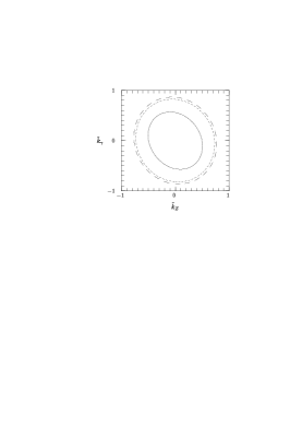
Figure 5: 95% C.L. bounds taking one coupling to be zero at a time and using the cuts of Eq. (4). The solid contours correspond to the bounds coming from the $p_{\mu}$ distribution, the short-dashed contours from the $\cos\theta$ distribution, and the long-dashed contours from the $p_{\mu\times\mu}$ distribution.

Since our bounds are probably limited by the low statistics, we now study the effect of relaxing the cuts, and impose only the minimal cut:

$$M_{\mu^{+}\mu^{-}}\geq 5\;~{}{\rm GeV}.$$ (9)

This is a very optimistic cut that still permits high efficiency in muon detection. Relaxing the cuts in this way has the effect of increasing the cross-section for the process $e^{+}e^{-}\to\mu^{+}\mu^{-}\nu\bar{\nu}$ to about 113 fb. With an integrated luminosity of 50 fb^-1 this results in 5660 events and consequently much better statistics.

In Figure 6 we present the total cross-section as a function of the anomalous coupling $g_{4}^{Z}$ (solid line), $\tilde{\kappa}_{Z}$ (short-dashed line) and $\tilde{\kappa}_{\gamma}$ (long-dashed line). Comparison with Figure 4 shows that the relaxed cuts increase the sensitivity to the anomalous couplings.

Figure 6: Total cross-section with the cuts of Eq. (9) as a function of $g_{4}^{Z}$ (solid line) and $\tilde{\kappa}_{Z,\gamma}$ (dashed-lines indistinguishable in this figure).

In Figure 7 we show the differential distributions with respect to the muon scattering angle, $\cos\theta$, and the muon momentum, $p_{\mu}$.

     

Figure 7: Standard model differential cross-section for the process $e^{+}e^{-}\rightarrow\mu^{+}\mu^{-}\nu\overline{\nu}$ at $\sqrt{s}=500$ GeV and the cuts in Eq. (9) as a function of a) $\cos\theta$ and b) $p_{\mu}$.

Once again we see that the standard model populates the regions of small scattering angle and low muon momentum preferentially. In Figure 8 we show the change in the differential cross-section when the anomalous couplings take values $g_{4}^{Z}=0.1$, $\tilde{\kappa}_{Z}=0.5$, and $\tilde{\kappa}_{\gamma}=0.5$. We take only one non-zero anomalous coupling at a time and use these values for illustration purposes only.

     

Figure 8: Deviations in differential cross-section with the cuts of Eq. (9) from their standard model values as a function of a) $\cos\theta$, b) $p_{\mu}$ and c) the $CP$ odd correlation of Eq. (6). In all cases the curves labeled 1, 2 and 3 correspond to $g_{4}^{Z}=0.1$, $\tilde{\kappa}_{Z}=0.5$ and $\tilde{\kappa}_{\gamma}=0.5$ respectively.

The standard model distribution is largest near $\theta=0$ whereas the new physics contributions are largest near $\theta=90^{o}$. Nevertheless, we find better sensitivity to the new physics when we do not impose the angular cut that excludes the region of small $\theta$, indicating that our analysis is limited by statistics.

To place bounds on the anomalous couplings, we use a standard $\chi^{2}$-criterion to analyze the events, include the anticipated 0.5% systematic error in the luminosity measurement, and take the muon identification efficiency to be 1. We find that the best bounds are achieved by dividing the events into 5 bins. The 95% C.L. results for $\sqrt{s}=500$ GeV, integrated luminosity of 50 fb^-1 and 5 bins for the bounds on $g_{4}^{Z}$, $\tilde{\kappa}_{Z}$, and $\tilde{\kappa}_{\gamma}$ are shown in Figure 9. In this figure we have taken one of the three couplings to be zero and looked at the projection of the allowed region into the plane of the other two couplings.

     

Figure 9: 95% C.L. bounds taking one coupling to be zero at a time and using the cuts of Eq. (9). The short-dashed contours correspond to the bounds coming from the $p_{\mu}$ distribution, the long-dashed contours from the $\cos\theta$ distribution, and the solid contours the $p_{\mu\times\mu}$ distribution.

In this figure the solid contours correspond to the bounds coming from the correlation $p_{\mu\times\mu}$, the short-dashed contours from the muon momentum distribution, and the long-dashed contours from the scattering angle distribution. Comparing Figures 5 and 9 one can see that with the relaxed cuts, the best bounds are obtained from the correlation $p_{\mu\times\mu}$. The improvement in the bounds is partly due to the increased statistics, and mostly due to the fact that when we relax the cut on the muon pair invariant mass we include a region of phase space that has the largest sensitivity to $p_{\mu\times\mu}$. In view of Eqs. (7) and (8), the region of smaller muon pair invariant mass ($M_{\mu^{+}\mu^{-}}<30$ GeV) appears to contain the region where $\sin\theta_{\mu}$ is large.

Alternatively, taking only one non-zero coupling at a time we find (from the correlation of Eq. (6)):

$$|\tilde{\kappa}_{\gamma}|\leq 0.27,\;|\tilde{\kappa}_{Z}|\leq 0.18,\;|g_{4}^{Z}|\leq 0.08.$$ (10)

4 Bounds from a $CP$-odd observable

In the previous section we have seen that the bounds that can be placed on the anomalous couplings using the correlation $p_{\mu\times\mu}$ are of the same order as those that can be placed from other observables. Therefore, it is interesting to see whether one can isolate the $CP$-odd components of the distributions with respect to $p_{\mu\times\mu}$, and in that way be able to really bound new $CP$ violating interactions.

To understand the effect of the different sets of cuts on these bounds we present in Figures 10 and 11 the differential cross-section with respect to the correlation $p_{\mu\times\mu}$ for $\tilde{\kappa}_{\gamma}=0.5$ and $\tilde{\kappa}_{Z}=0.5$ respectively.

     

Figure 10: Deviations in the differential cross-section with a) the cuts of Eq. (4) and b) the cuts of Eq. (9) as a function of $p_{\mu\times\mu}$ for $\tilde{\kappa}_{\gamma}=0.5$. We have separated the contribution from the term linear in $\tilde{\kappa}_{\gamma}$ (antisymmetric curve) from that due to the term quadratic in $\tilde{\kappa}_{\gamma}$ (symmetric curve).

     

Figure 11: Deviations in the differential cross-section with a) the cuts of Eq. (4) and b) the cuts of Eq. (9) as a function of $p_{\mu\times\mu}$ for $\tilde{\kappa}_{Z}=0.5$. We have separated the contribution from the term linear in $\tilde{\kappa}_{Z}$ (antisymmetric curve) from that due to the term quadratic in $\tilde{\kappa}_{Z}$ (symmetric curve).

In these figures we have separated the contributions to the differential cross-section arising from terms linear in the anomalous couplings (the curves that are antisymmetric about $p_{\mu\times\mu}=0$) from those arising from terms quadratic in the anomalous couplings (the curves that are symmetric about $p_{\mu\times\mu}=0$). We also show how these results vary when we go from the stronger cuts of Eq. (4) to the relaxed cut of Eq. (9).

Notice that the normalization of the curves with strong and weak cuts is different as it corresponds to the respective total cross-section. From these curves we see that the relaxed cuts are not only better because they increase the statistics, but they also increase the relative contribution of the truly $CP$-odd term linear in $\tilde{\kappa}_{\gamma,Z}$ as we argued in the previous section.

In order to quantify the bounds that can be placed in this way, we introduce the integrated $CP$-odd observable

$$A\equiv\int{d\sigma\over dp_{\mu\times\mu}}\cdot\mbox{sign}(p_{\mu\times\mu})dp_{\mu\times\mu}.$$ (11)

Specifically we take the $\mbox{sign}(p_{\mu\times\mu})$ to be zero if $p_{\mu\times\mu}=0$ to exclude that point, and use the following criterion to place bounds;

$$|\int\frac{d\sigma}{dp_{\mu\times\mu}}\cdot\mbox{sign}(p_{\mu\times\mu})dp_{\mu\times\mu}|\leq 2\cdot\Delta\sigma_{exp}\;.$$ (12)

The right-hand side of this equation corresponds to two standard deviations for the experimentally measured cross-section. Given the definition of $A$ it is appropriate to use the same experimental uncertainty of the total cross-section:

$$\Delta\sigma_{exp}=\sigma_{SM}\cdot\sqrt{\delta^{2}_{syst}+\delta^{2}_{stat}}\;,$$ (13)

where

$$\delta_{stat}=\frac{1}{\sqrt{\sigma_{SM}\cdot\cal{L}\cdot\epsilon_{\mu}}}\;.$$ (14)

The best bounds come from using the relaxed cut of Eq. (9) and are given by

$$|\tilde{k}_{Z}+0.7\cdot\tilde{k}_{\gamma}|\leq 0.2$$ (15)

It is also possible to obtain bounds on $g_{4}^{Z}$ but they are much weaker.

5 Conclusions

We have studied the effect of $CP$ violating anomalous couplings on the process $e^{+}e^{-}\rightarrow W^{+}W^{-}$. Using $CP$ even observables we have found that a NLC with $\sqrt{s}=500$ GeV and $50$ pb^-1 can place the bounds $|\tilde{\kappa}_{\gamma,Z}|\leq 0.1$ and $|g_{4}^{Z}|\leq 0.09$. These bounds are comparable to those that can be placed with an upgraded Tevatron, and are of the same order as the bounds that can be placed on $CP$ conserving anomalous couplings. These bounds originate in the quadratic contributions of the couplings to the differential cross-section. By looking at the $\mu\nu$ decays of the $W$-bosons we were able to construct a $CP$ odd correlation that can directly bound the $CP$-violating terms (linear in the couplings) in the differential cross-section. We found that it will be possible to place the bounds $|\tilde{\kappa}_{\gamma}|\leq 0.3$ and $|\tilde{\kappa}_{Z}|\leq 0.2$. We conclude that the sensitivity of a NLC to $CP$ violating anomalous couplings is similar to its sensitivity to $CP$ conserving anomalous couplings. From our dimensional analysis we also conclude that it is unlikely that $CP$ violating anomalous couplings will be seen by a NLC unless the smallness of $\Delta\rho$ is accidental.

Acknowledgments The work of A.A.L and O.P.Y. was supported in part by RFBR under grant number 96-02-18216. The work of G.V. was supported in part by the DOE OJI program under contract number DEFG0292ER40730. We thank S. Dawson for comments on the manuscript.

References

- [1] See for example H. Aihara et. al. in Electroweak Symmetry Breaking and New Physics at the TeV Scale, World Scientific (1996) and references therein.
- [2] K. Hagiwara et. al., Nucl. Phys. B282 253 (1987); K. Gaemers and G. Gounaris, Z. Phys. C1, 259 (1979).
- [3] T. Appelquist and C. Bernard, Phys. Rev. D22 200 (1980); A. Longhitano, Nucl. Phys. B188 118 (1981); C. P. Burgess and J. A. Robinson, BNL Summer Study on CP Violation 205 (1990); T. Appelquist and G.-H. Wu, Phys. Rev. D48 3235 (1993).
- [4] T. Appelquist and G. H. Wu, Phys. Rev. D51, 240 (1995).
- [5] S. Dawson and G. Valencia, Phys. Rev. D49, 2188 (1994).
- [6] This is an updated number from Ref. [4] that uses the result of W. Marciano and A. Quejeiro, Phys. Rev. D33, 3449 (1986).
- [7] S. Dawson and G. Valencia, Phys. Rev. D52, 2717 (1995); S. Dawson, Xiao-Gang He and G. Valencia, Phys. Lett. B390, 431 (1997).
- [8] G. Gounaris, D. Schildknecht and F. M. Renard, Phys. Lett. B263, 291 (1991); F. Boudjema et. al., Phys. Rev. D43 3683 (1991); D. Chang, W.-Y. Keung and I. Phillips, Phys. Rev. D48, 4045 (1993); D. Choudhury and S. Rindani, Phys. Lett. B335 198 (1994); G. Gounaris and C. Papadopoulos, hep-ph/9612378.
- [9] S. Rindani and J. P. Singh, hep-ph/9703380.
- [10] M. Frank et al., in proceedings of Workshop “ collisions at 500 GeV: the Physics Potential”, ed. P.M.Zerwas DESY Hamburg, 223 (1991); G. Gounaris et al., in proceedings of Workshop “ collisions at 500 GeV: the Physics Potential”, ed. P.M.Zerwas DESY Hamburg, 735 (1991).
- [11] A. A. Likhoded, T. Han and G. Valencia, Phys. Rev. D53, 4811 (1996). A similar study can be found in V. V. Andreev, A. A. Pankov, and N. Paver, Phys. Rev. D53, 2390 (1996).
- [12] J. F. Donoghue and G. Valencia, Phys. Rev. Lett. 58,451 (1987), Erratum-ibid.60,243 (1988).
- [13] A.A.Likhoded et al., Phys. Atom. Nucl. 58 (1995), p. 243.