ELECTROWEAK THEORY AND
THE 1996/97 PRECISION ELECTROWEAK DATA

Abstract

We review the empirical evidence for the validity of the Standard Electroweak Theory in Nature. The experimental data are interpreted in terms of an effective Lagrangian for Z physics, allowing for potential sources of SU(2) violation and containing the predictions of the Standard Electroweak Theory as a special case. Particular emphasis is put on discriminating loop corrections due to fermion-loop vector-boson propagator corrections on the one hand, from corrections depending on the non-Abelian structure and the Higgs sector on the other hand. Results from recently obtained fits of the Higgs-boson mass are reported, yielding $M_{\mathrm{H}}\>\raisebox{-2.15277pt}{$\stackrel{{\scriptstyle\textstyle<}}{{\sim}}$}\>430$ GeV [680 GeV] at 95% C.L. based on the input of $\bar{s}_{\scriptscriptstyle{\mathrm{W}}}^{2}({\mathrm{LEP}}+{\mathrm{SLD}})_{`97}~{}=0.23152\pm 0.00023$ [$\bar{s}_{\scriptscriptstyle{\mathrm{W}}}^{2}({\mathrm{LEP}})_{`97}~{}=0.23196\pm 0.00028$]. The LEP2 data provide first direct experimental evidence for non-zero non-Abelian couplings among the electroweak vector bosons.

1 Z Physics

The spirit in which I will look at the electroweak precision data may be characterized by quoting Feynman who once said:

” In any event, it is always a good idea to try to see how much or how little of our theoretical knowledge actually goes into the analysis of those situations which have been experimentally checked.” R.P. Feynman [2]

1.1 The $\alpha(0)$-Born Prediction

The quality of the data on electroweak interactions may be particularly well appreciated by starting with an analysis in terms of the Born approximation of the Standard Electroweak Theory (Standard Model, SM) [3, 4]. From the input of

$$\alpha(0)^{-1} = 137.0359895(61),\qquad G_{\mu}=1.16639(2)\cdot 10^{-5}{\rm GeV}^{-2},$$

$$M_{\mathrm{Z}} = 91.1863\pm 0.0020{\rm GeV},$$ (1)

one may predict the partial width of the Z for decay into leptons, $\Gamma_{\mathrm{l}}$, the weak mixing angle, $\bar{s}_{\scriptscriptstyle{\mathrm{W}}}^{2}$, and the $W$ mass, $M_{\mathrm{W}}$. The $\alpha(0)$-Born approximation, in distinction from the $\alpha(M_{\mathrm{Z}}^{2})$-Born approximation to be introduced below,

$$\bar{s}_{\scriptscriptstyle{\mathrm{W}}}^{2}(1-\bar{s}_{\scriptscriptstyle{\mathrm{W}}}^{2}) = \frac{\pi\alpha(0)}{\sqrt{2}G_{\mu}M_{\mathrm{Z}}^{2}},$$

$$\Gamma_{\mathrm{l}} = \frac{G_{\mu}M^{3}_{Z}}{24\pi\sqrt{2}}\left(1+(1-4\bar{s}_{\scriptscriptstyle{\mathrm{W}}}^{2})^{2}\right),$$

$$M_{\mathrm{W}}^{2} = M_{\mathrm{Z}}^{2}(1-\bar{s}_{\scriptscriptstyle{\mathrm{W}}}^{2}),$$ (2)

then yields

$$\bar{s}_{\scriptscriptstyle{\mathrm{W}}}^{2}=0.2121,\qquad\Gamma_{\mathrm{l}}=84.85~{}{\rm MeV},\qquad M_{\mathrm{W}}=80.940~{}{\rm GeV}.$$ (3)

A comparison with the experimental data from tab. 1,

$$\bar{s}_{\scriptscriptstyle{\mathrm{W}}}^{2}({\mathrm{LEP}}+{\mathrm{SLD}}) = 0.23165\pm 0.00024,\qquad\Gamma_{\mathrm{l}}=83.91\pm 0.11\,\mathrm{MeV},$$

$$M_{\mathrm{W}} = 80.356\pm 0.125\,\mathrm{GeV},$$ (4)

shows discrepancies between the $\alpha(0)$-Born approximation and the data by many standard deviations.

leptonic sector	hadronic sector
$\Gamma_{\mathrm{l}}=83.91\pm 0.11\,\mathrm{MeV}$	$\begin{array}[]{rr}R=20.778~{}~{}\pm&0.029\\ 75~{}~{}\pm&27\end{array}$
$\begin{array}[]{rr}\bar{s}_{\scriptscriptstyle{\mathrm{W}}}^{2}|_{{\mathrm{LEP}}}=0.23200~{}~{}\pm&0.00027\\ 196~{}~{}\pm&28\end{array}$	$\begin{array}[]{rr}\Gamma_{\mathrm{T}}=2494.6~{}~{}\pm&2.7\,\mathrm{MeV}\\ .8~{}~{}\pm&2.5\phantom{\,\mathrm{MeV}}\end{array}$
$\begin{array}[]{rr}\bar{s}_{\scriptscriptstyle{\mathrm{W}}}^{2}|_{{\mathrm{SLD}}}=0.23061~{}~{}\pm&0.00047\\ 55~{}~{}\pm&41\\ \end{array}$	$\begin{array}[]{rr}\sigma_{\mathrm{h}}=41.508~{}~{}\pm&0.056\\ 486~{}~{}\pm&53\\ \end{array}$
$\begin{array}[]{rr}\bar{s}_{\scriptscriptstyle{\mathrm{W}}}^{2}|_{\mathrm{LEP+SLD}}=0.23165~{}~{}\pm&0.00024\\ 52~{}~{}\pm&23\\ \end{array}$	$\begin{array}[]{rr}\Gamma_{\mathrm{h}}=1743.6~{}~{}\pm&2.5\,\mathrm{MeV}\\ .1~{}~{}\pm&.3\phantom{MeV}\\ \end{array}$
$\begin{array}[]{rr}M_{\mathrm{W}}=80.356~{}~{}\pm&0.125\,\mathrm{GeV}\\ 430~{}~{}\pm&80\phantom{\,\mathrm{GeV}}\\ \end{array}$	$\begin{array}[]{rr}R_{\mathrm{b}}=0.2179~{}~{}\pm&0.0012\\ 74~{}~{}\pm&9\\ \end{array}$
	$\Gamma_{\mathrm{b}}=379.9~{}~{}\pm~{}~{}2.2\,\mathrm{MeV}$
	$\begin{array}[]{rr}R_{\mathrm{c}}=0.1715~{}~{}\pm&0.0056\\ 27~{}~{}\pm&50\\ \end{array}$
	$\Gamma_{\mathrm{c}}=299.0~{}~{}\pm~{}~{}9.8\,\mathrm{MeV}$
input parameters	correlation matrices
$\begin{array}[]{c}\begin{array}[]{rr}M_{\mathrm{Z}}=91.1863~{}~{}\pm&0.0020\,\mathrm{GeV}\\ 67~{}~{}\pm&20\phantom{\,\mathrm{GeV}}\end{array}\\ \hline\cr G_{\mu}=1.16639(2)\cdot 10^{-5}\,\mathrm{GeV}^{-2}\\ \hline\cr\alpha(M_{\mathrm{Z}}^{2})^{-1}=128.89\pm 0.09\\ \hline\cr\alpha_{\mathrm{s}}(M_{\mathrm{Z}}^{2})=0.123\pm 0.006\\ \hline\cr m_{\mathrm{b}}=4.7\,\mathrm{GeV}\\ \hline\cr\begin{array}[]{rr}m_{\mathrm{t}}=175\phantom{.6}~{}~{}\pm&6\phantom{.5}\,\mathrm{GeV}\\ 5.6~{}~{}\pm&5.5\phantom{\,\mathrm{GeV}}\end{array}\end{array}$	$\begin{array}[]{c}\rule{0.0pt}{66.86397pt}\begin{array}[b]{|c||c|c|c|c|}\hline\cr&\sigma_{\mathrm{h}}&R&\Gamma_{\mathrm{T}}\\ \hline\cr\hline\cr\sigma_{\mathrm{h}}&\phantom{-}1.00&\phantom{-}0.15&-0.14\\ \hline\cr R&\phantom{-}0.15&\phantom{-}1.00&-0.01\\ \hline\cr\Gamma_{\mathrm{T}}&-0.14&-0.01&\phantom{-}1.00\\ \hline\cr\end{array}\\ \begin{array}[b]{|c||c|c|c|}\hline\cr&R_{\mathrm{b}}&R_{\mathrm{c}}\\ \hline\cr\hline\cr R_{\mathrm{b}}&\phantom{-}1.00&-0.23\\ \hline\cr R_{\mathrm{c}}&-0.23&\phantom{-}1.00\\ \hline\cr\end{array}\end{array}$

Table 1: The 1996 precision data (and below these data the last digits of the 1997 data), consisting of the LEP data [5], the SLD value [6, 5] for $\bar{s}_{\scriptscriptstyle{\mathrm{W}}}^{2}$, and the world average [7, 5] for $M_{\mathrm{W}}$. The partial widths $\Gamma_{\mathrm{l}}$, $\Gamma_{\mathrm{h}}$, $\Gamma_{\mathrm{b}}$, and $\Gamma_{\mathrm{c}}$ are obtained from the observables $R=\Gamma_{\mathrm{h}}/\Gamma_{\mathrm{l}}$, $\sigma_{\mathrm{h}}=(12\pi\Gamma_{\mathrm{l}}\Gamma_{\mathrm{h}})/(M_{\mathrm{Z}}^{2}\Gamma^{2}_{\mathrm{T}})$, $R_{\mathrm{b}}=\Gamma_{\mathrm{b}}/\Gamma_{\mathrm{h}}$, $R_{\mathrm{c}}=\Gamma_{\mathrm{c}}/\Gamma_{\mathrm{h}}$, and $\Gamma_{\mathrm{T}}$ using the given correlation matrices. The data in the upper left-hand column will be referred to as “leptonic sector” subsequently. Inclusion of the data in the upper right-hand column will be referred to as “all data”. If not stated otherwise, the SM predictions will be based on the input parameters given in the lower left-hand column of the table, where $\alpha(M_{\mathrm{Z}}^{2})$ is taken from Ref. [8], $\alpha_{\mathrm{s}}(M_{\mathrm{Z}}^{2})$ results from the event-shape analysis [9] at LEP, and $m_{\mathrm{t}}$ represents the direct Tevatron measurement [10]. Note that the difference between the 1996 and the 1997 data is half a standard deviation at most.

1.2 The $\alpha(M_{\mathrm{Z}}^{2})$-Born, the Full Fermion-Loop and the Complete One-Loop Standard Model Predictions

Turning to corrections to the $\alpha(0)$-Born approximation, I follow the 1988 strategy “to isolate and to test directly the ’new physics’ of boson loops and other new phenomena by comparing with and looking for deviations from the predictions of the dominant-fermion-loop results” [11]. Accordingly, let us strictly discriminate [12, 13, 14, 15, 16] vacuum-polarization contributions due to fermion loops in the photon, $Z$ and $W$ propagators from all other loop corrections, the “bosonic” loops, which contain virtual vector bosons within the loops. I note that this distinction between two classes of loop corrections is gauge invariant in the SU(2)${}_{L}\times$U(1)_Y electroweak theory. Otherwise the theory would fix the number of fermion families. The reason for systematically discriminating fermion loops in the propagators from the rest is in fact obvious. The fermion-loop effects, leading to “running” of coupling constants and to mixing among the neutral vector bosons, can be precisely predicted from the empirically known couplings of the leptons and the (light) quarks, while other loop effects, such as vacuum polarization due to boson pairs and vertex corrections, depend on the empirically unknown couplings among the vector bosons and the properties of the Higgs scalar. It is in fact the difference between the fermion-loop predictions and the full one-loop results which sets the scale [11] for the precision required for empirical tests of the electroweak theory beyond (trivial) fermion-loop effects. One should remind oneself that the experimentally unknown bosonic interactions are right at the heart of the celebrated renormalizability properties [17] of the electroweak non-Abelian gauge theory [4].

When considering fermion loops, let us first of all look at the contributions of leptons and quarks to the photon propagator. Vacuum polarization due to leptons and quarks, or rather hadrons in the latter case, leads to the well-known increase (“running”) of the electromagnetic coupling as a function of the scale at which it is measured. While the contribution of leptons can be calculated in a straightforward manner, the one of quarks is more reliably obtained from the cross section for $e^{+}e^{-}\to$ hadrons via a dispersion relation [8, 18]. As a consequence of the experimental errors in this cross section, in particular in the region below about $3.5\,\mathrm{GeV}$, the value of the electromagnetic fine-structure constant at the $Z$ scale, relevant for LEP1 physics, contains a non-negligible error,

$$\alpha(M_{\mathrm{Z}}^{2})^{-1}=128.89\pm 0.09.$$ (5)

Replacing $\alpha(0)$ in (2) by $\alpha(M_{\mathrm{Z}}^{2})$ implies replacing $\bar{s}_{\scriptscriptstyle{\mathrm{W}}}^{2}$ in (2) by $s^{2}_{0}$,

$$s^{2}_{0}(1-s^{2}_{0})=\frac{\pi\alpha(M_{\mathrm{Z}}^{2})}{\sqrt{2}G_{\mu}M_{\mathrm{Z}}^{2}},$$ (6)

which may be expected to be a more appropriate parameter for electroweak physics at the Z-boson scale than the mixing angle from the $\alpha(0)$-Born approximation (2). As the transition from $\alpha(0)$ to $\alpha(M_{\mathrm{Z}}^{2})$ is an effect purely due to the electromagnetic interactions of leptons and quarks (hadrons), even present in the absence of weak interactions, the relations (2) with the replacement $s^{2}_{W}\rightarrow s^{2}_{0}$ from (6) may appropriately be called the “$\alpha(M_{\mathrm{Z}}^{2})$-Born approximation” [19] of the electroweak theory.

Figure 1: Three-dimensional plot of the $1\sigma$ ellipsoid of the 1996 experimental data in ($M_{\mathrm{W^{\pm}}}/M_{\mathrm{Z}}$, $\bar{s}_{\scriptscriptstyle{\mathrm{W}}}^{2}$, $\Gamma_{\mathrm{l}}$)-space, using $\bar{s}_{\scriptscriptstyle{\mathrm{W}}}^{2}$ (LEP + SLD) as experimental input for $\bar{s}_{\scriptscriptstyle{\mathrm{W}}}^{2}$, in comparison with the full SM prediction (connected lines) and the pure fermion-loop prediction (single line with cubes). The full SM prediction is shown for Higgs-boson masses of $M_{\mathrm{H}}=100\,\mathrm{GeV}$ (line with diamonds), $300\,\mathrm{GeV}$, and $1\,\mathrm{TeV}$ parametrized by $m_{\mathrm{t}}$ ranging from 120–220$\,\mathrm{GeV}$ in steps of $20\,\mathrm{GeV}$. In the pure fermion-loop prediction the cubes also indicate steps in $m_{\mathrm{t}}$ of $20\,\mathrm{GeV}$ starting with $m_{\mathrm{t}}=120$ $\,\mathrm{GeV}$. The cross outside the ellipsoid indicates the $\alpha(M_{\mathrm{Z}}^{2})$-Born approximation with the corresponding error bars, which also apply to all other SM predictions (1996 update from Ref. [16]). Note that in the projections on the planes also the $2\sigma$ contours are shown.

Numerically, one finds

$$s^{2}_{0} = 0.23112\pm 0.00023,$$

$$\Gamma_{\mathrm{l}}^{(0)} = 83.563\pm 0.012~{}{\rm MeV},$$

$$M^{(0)}_{{\mathrm{W}}} = 79.958\pm 0.011~{}{\rm GeV},$$ (7)

i.e. a large part of the discrepancy between the predictions (3) and the data (4) is due to the use of the inappropriate value of $\alpha(0)$, instead of $\alpha(M_{\mathrm{Z}}^{2})$, as appropriate for Z physics. Note that the uncertainty in $s^{2}_{0}$, as a consequence of the error in $\alpha(M_{\mathrm{Z}}^{2})$, is as large as the error of $\bar{s}_{\scriptscriptstyle{\mathrm{W}}}^{2}$ from the measurements at the Z resonance (compare (4) or tab. 1).

All other fermion-loop effects are due to fermion loops in the W propagator (relevant simce $G_{\mu}$ enters the predictions) and in the Z propagator, and due to the important effect of $\gamma$Z mixing induced by fermions. Light fermions as well as the top quark accordingly yield important contributions to the “full fermion-loop prediction” which includes all fermion-loop propagator corrections.

In fig. 1, an update of a figure in Ref. [16], we show the experimental data from the “leptonic sector”, $\bar{s}^{2}_{W},\Gamma_{\mathrm{l}},M_{\mathrm{W}}$, in comparison with the $\alpha(M_{\mathrm{Z}}^{2})$-Born approximation, the full fermion-loop prediction, and the complete one-loop Standard Model results. Note that fig. 1 shows the 1996 data. According to tab. 1, the difference between the 1997 data [4] and the 1996 data is much below one standard deviation and irrelevant for the content of fig. 1 and most of the further conclusions.
We conclude that [16, 14],

• contributions beyond the $\alpha(M_{\mathrm{Z}}^{2})$-Born approximation are needed for agreement with the data,

• contributions beyond the full fermion-loop predictions, based on $\alpha(M_{\mathrm{Z}}^{2})$, the fermion-loop contributions to the $W$ and $Z$ propagators and to $\gamma Z$ mixing, and the top quark effects, are necessary, and provided

• by additional contributions involving bosonic loops, dependent on the non-Abelian couplings and the properties of the Higgs boson.

The increase in precision of the experimental data may be particularly well appreciated by comparing with the results which I discussed at the XVII International School of Theoretical Physics in Szczyrk, in September 1993 [20].

The question immediately arises of what can be said in more detail about the various contributions due to fermionic and bosonic loops, leading to the final agreement between theory and experiment.

1.3 Effective Lagrangian, $\Delta x,\Delta y,\varepsilon,\Delta y_{\mathrm{b}}$ Parameters

This question can be answered by an analysis in terms of the parameters $\Delta x,\Delta y$ and $\varepsilon$ which within the framework of an effective Lagrangian [13, 14, 15] specify potential sources of SU(2) violation. The “mass parameter” $\Delta x$ is related to SU(2) violation by the masses of the triplet of charged and neutral (unmixed) vector boson via

$$M_{\mathrm{W}}^{2}\equiv(1+\Delta x)M^{2}_{W^{0}}\equiv xM^{2}_{W^{0}},$$ (8)

while the “coupling parameter” $\Delta y$ specifies SU(2) violation among the $W^{\pm}$ and $W^{0}$ couplings to fermions,

$$g^{2}_{W^{\pm}}(0)\equiv M^{2}_{W^{\pm}}4\sqrt{2}G_{\mu}=(1+\Delta y)g^{2}_{W^{0}}(M_{\mathrm{Z}}^{2})\equiv yg^{2}_{W^{0}}(M_{\mathrm{Z}}^{2}).$$ (9)

Finally, the “mixing parameter” $\varepsilon$ refers to the mixing strength in the neutral vector boson sector and quantifies the deviation of $\bar{s}_{\scriptscriptstyle{\mathrm{W}}}^{2}$ from $e^{2}(M_{\mathrm{Z}}^{2})/g^{2}_{W^{0}}(M_{\mathrm{Z}}^{2})$,

$$\bar{s}_{\scriptscriptstyle{\mathrm{W}}}^{2}\equiv\frac{e^{2}(M_{\mathrm{Z}}^{2})}{g^{2}_{W^{0}}(M_{\mathrm{Z}}^{2})}(1-\varepsilon),$$ (10)

thus allowing for an unconstrained mixing strength [12, 21] in the neutral vector-boson sector. The effective Lagrangian incorporating the mentioned sources of SU(2) violation for $W$ and $Z$ interactions with leptons is given by [14, 13]

$${\cal L}_{C}=-\frac{1}{2}W^{+\mu\nu}W^{-}_{\mu\nu}+\frac{g_{\mathrm{W^{\pm}}}}{\sqrt{2}}\left(j^{+}_{\mu}W^{+\mu}+h.c.\right)+M_{\mathrm{W^{\pm}}}^{2}W^{+}_{\mu}W^{-\mu}$$ (11)

and

$${\cal L}_{N} = -\frac{1}{4}Z_{\mu\nu}Z^{\mu\nu}+\frac{1}{2}\frac{M_{\mathrm{W^{0}}}^{2}}{1-\bar{s}_{\scriptscriptstyle{\mathrm{W}}}^{2}(1-\varepsilon)}Z_{\mu}Z^{\mu}-\frac{1}{4}A_{\mu\nu}A^{\mu\nu}$$ (12)

$$-ej_{em}^{\mu}A_{\mu}+\frac{g_{\mathrm{W^{0}}}}{\sqrt{1-\bar{s}_{\scriptscriptstyle{\mathrm{W}}}^{2}(1-\varepsilon)}}\left(j^{\mu}_{3}-\bar{s}_{\scriptscriptstyle{\mathrm{W}}}^{2}j^{\mu}_{em}\right)Z_{\mu}.$$

For the observables $\bar{s}_{\scriptscriptstyle{\mathrm{W}}}^{2},M_{\mathrm{W}}$ and $\Gamma_{\mathrm{l}}$, from (11) and (12) one obtains

$$\bar{s}_{\scriptscriptstyle{\mathrm{W}}}^{2}(1-\bar{s}_{\scriptscriptstyle{\mathrm{W}}}^{2}) = {{\pi\alpha(M_{\mathrm{Z}}^{2})}\over{\sqrt{2}G_{\mu}M_{\mathrm{Z}}^{2}}}{y\over x}(1-\varepsilon){1\over{\left(1+{\bar{s}_{\scriptscriptstyle{\mathrm{W}}}^{2}\over{1-\bar{s}_{\scriptscriptstyle{\mathrm{W}}}^{2}}}\varepsilon\right)}},$$

$${M_{\mathrm{W}}^{2}\over M_{\mathrm{Z}}^{2}} = (1-\bar{s}_{\scriptscriptstyle{\mathrm{W}}}^{2})x\left(1+{\bar{s}_{\scriptscriptstyle{\mathrm{W}}}^{2}\over{1-\bar{s}_{\scriptscriptstyle{\mathrm{W}}}^{2}}}\varepsilon\right),$$

$$\Gamma_{\mathrm{l}} = {{G_{\mu}M^{3}_{Z}}\over{24\pi\sqrt{2}}}\left(1+(1-4\bar{s}_{\scriptscriptstyle{\mathrm{W}}}^{2})^{2}\right){x\over y}\left(1-{{3\alpha}\over{4\pi}}\right).$$ (13)

For $x=y=1$ (i.e., $\Delta x=\Delta y=0$) and $\varepsilon=0$ one recovers the $\alpha(M_{\mathrm{Z}}^{2})$-Born approximation, $\bar{s}_{\scriptscriptstyle{\mathrm{W}}}^{2}=s^{2}_{0}$, discussed previously.

The extension [15] of the effective Lagrangian (12) to interactions of neutrinos and quarks requires the additional coupling parameters $\Delta y_{\nu}$ for the neutrino, $\Delta y_{b}$ for the bottom quark, and $\Delta y_{h}$ for the remaining light quarks. In the analysis of the data, for $\Delta y_{\nu}$ and $\Delta y_{h}$ which do not involve the non-Abelian structure of the theory, the SM theoretical results may be inserted without loss of generality as far as the guiding principle of separating vector-boson–fermion interactions from interactions containing non-Abelian couplings is concerned.

We note that the parameters in our effective Lagrangian are related [15] to the parameters $\varepsilon_{1,2,3}$ and $\epsilon_{b}$, introduced [22] by isolating the quadratic $m_{\mathrm{t}}$ dependence,

$$\varepsilon_{1}=\Delta x-\Delta y+0.2\times 10^{-3}, \varepsilon_{2}=-\Delta y+0.1\times 10^{-3},$$

$$\varepsilon_{3}=-\varepsilon+0.2\times 10^{-3}, \varepsilon_{\mathrm{b}}=-\Delta y_{\mathrm{b}}/2-0.1\times 10^{-3}.$$ (14)

Essentially the two sets of parameters only differ in $\varepsilon_{1}$. As $\varepsilon_{1}$ contains a linear combination of $\Delta x$ and $\Delta y$, the $M_{\mathrm{H}}$-dependent bosonic corrections in $\Delta x$ are confused with the $M_{\mathrm{H}}$-insensitive bosonic corrections in $\Delta y$, i.e. with our choice of parameters the $M_{H}$-insensitive corrections are isolated and appear in the single parameter $\Delta y$ only. The theoretically interesting, but numerically irrelevant additive terms in (14), considerably smaller than $1\times 10^{-3}$, originate from a refinement in the mixing involved in Lagrangian (12) and a corresponding refinement in (13). We refer to the original paper [15] for details.

By linearizing the equations in (13) with respect to $\Delta x,\Delta y$ and $\varepsilon$ and inverting them, $\Delta x,\Delta y$ and $\varepsilon$ may be deduced from the experimental data on $\bar{s}_{\scriptscriptstyle{\mathrm{W}}}^{2},\Gamma_{\mathrm{l}}$ and $M_{\mathrm{W}}$. Inclusion of the hadronic $Z$ observables requires that $\Delta x,\Delta y,\varepsilon$ and $\Delta y_{b}$ are fitted to the experimental data. Actually, one finds that the results for $\Delta x,\Delta y,\varepsilon$ are hardly affected by inclusion of the hadronic observables. On the other hand, $\Delta x,\Delta y,\varepsilon$ and $\Delta y_{b}$ may be theoretically determined in the standard electroweak theory at the one-loop level, strictly discriminating between pure fermion-loop predictions and the rest which contains the unknown bosonic couplings. The most recent 1996 update [23] of such an analysis [16, 14, 15] is shown in fig. 2.

Figure 2: The projections of the $1\sigma$ ellipsoid of the electroweak parameters $\Delta x$, $\Delta y$, $\varepsilon$, $\Delta y_{\mathrm{b}}$ obtained from the 1996 set of data in comparison with the SM predictions. Both the results obtained from using $\bar{s}_{\scriptscriptstyle{\mathrm{W}}}^{2}({\mathrm{LEP}})$ and $\bar{s}_{\scriptscriptstyle{\mathrm{W}}}^{2}({\mathrm{LEP}}+{\mathrm{SLD}})$ as experimental input are shown. The full SM predictions correspond to Higgs-boson masses of $100\,\mathrm{GeV}$ (dotted with diamonds), $300\,\mathrm{GeV}$ (long-dashed dotted) and $1\,\mathrm{TeV}$ (short-dashed dotted) parametrized by the top-quark mass ranging from $120\,\mathrm{GeV}$ to $220\,\mathrm{GeV}$ in steps of $20\,\mathrm{GeV}$. The pure fermion-loop prediction is also shown (short-dashed curve with squares) for the same values of $m_{\mathrm{t}}$. The arrows indicate the shifts of the centres of the ellipses upon changing $\alpha(M_{\mathrm{Z}}^{2})^{-1}$ to $\alpha(M_{\mathrm{Z}}^{2})^{-1}+\delta\alpha(M_{\mathrm{Z}}^{2})^{-1}$ and $\alpha_{\mathrm{s}}(M_{\mathrm{Z}}^{2})$ to $\alpha_{\mathrm{s}}(M_{\mathrm{Z}}^{2})+\delta\alpha_{\mathrm{s}}(M_{\mathrm{Z}}^{2})$. (From Ref. [23])

According to fig. 2, the data in the $(\varepsilon,\Delta x)$ plane are consistent with the SM predictions obtained by approximating $\Delta x$ and $\varepsilon$ by their pure fermion-loop values,

$$\Delta x = \Delta x_{{\rm ferm}}(\alpha(M_{\mathrm{Z}}^{2}),s^{2}_{0},m_{\mathrm{t}}^{2}\ln m_{\mathrm{t}})+\Delta x_{{\rm bos}}(\alpha(M_{\mathrm{Z}}^{2}),s^{2}_{0},\ln M_{\mathrm{H}}^{2})$$

$$\cong \Delta x_{{\rm ferm}}(\alpha(M_{\mathrm{Z}}^{2}),s^{2}_{0},m_{\mathrm{t}}^{2},\ln m_{\mathrm{t}}),$$

$$\varepsilon = \varepsilon_{{\rm ferm}}(\alpha(M_{\mathrm{Z}}^{2}),s^{2}_{0},\ln m_{\mathrm{t}})+\varepsilon_{{\rm bos}}(\alpha(M_{\mathrm{Z}}^{2}),s^{2}_{0},\ln M_{\mathrm{H}}^{2})$$ (15)

$$\cong \varepsilon_{{\rm ferm}}(\alpha(M_{\mathrm{Z}}^{2}),s^{2}_{0},\ln m_{\mathrm{t}}).$$

The small contributions of $\Delta x_{{\rm bos}}$ and $\varepsilon_{{\rm bos}}$ to $\Delta x$ and $\varepsilon$, respectively, and the logarithmic dependence on the Higgs mass, $M_{\mathrm{H}}$, imply the well-known result that the data are fairly insensitive to the mass of the Higgs scalar. It is instructive to also note the numerical results for $\Delta x_{{\rm ferm}}$ and $\varepsilon_{{\rm ferm}}$, obtained in the Standard Model. They are given by [14]

$$\Delta x_{{\rm ferm}} = (2.61t+1.34\log(t)+0.52)\times 10^{-3},$$

$$\varepsilon_{{\rm ferm}} = (-0.45\log(t)-6.43)\times 10^{-3},$$ (16)

with $t\equiv m_{\mathrm{t}}^{2}/M_{\mathrm{Z}}^{2}$. The mass parameter $\Delta x$ is dominated by the $m_{\mathrm{t}}^{2}$ term [24] due to weak isospin breaking induced by the top quark, while $\varepsilon$ is dominated by the constant term due to mixing among the neutral vector bosons induced by the light leptons and quarks.

In distinction from the results for $\Delta x$ and $\varepsilon$, where the fermion loops by themselves are consistent with the data, a striking effect appears in the plots showing $\Delta y$. The predictions are clearly inconsistent with the data, unless the fermion-loop contributions to $\Delta y$ (denoted by lines with small squares) are supplemented by an additional term, which in the standard electroweak theory is due to bosonic effects,

$$\Delta y=\Delta y_{{\rm ferm}}(\alpha(M_{\mathrm{Z}}^{2}),s^{2}_{0},\ln m_{\mathrm{t}})+\Delta y_{{\rm bos}}(\alpha(M_{\mathrm{Z}}^{2}),s^{2}_{0}).$$ (17)

Remembering that $\Delta y$, according to (9), relates the coupling of the $W^{\pm}$ boson to leptons as measured in $\mu^{\pm}$ decay, to the coupling of the neutral member, $W^{0}$, of the vector-boson triplet at the scale $M_{\mathrm{Z}}$, it is not surprising that $\Delta y_{{\mathrm{bos}}}$ contains vertex and box corrections originating from $\mu^{\pm}$ decay as well as vertex corrections at the $W^{0}f\bar{f}$ ($Zf\bar{f}$) vertex. While $\Delta y_{{\rm bos}}$ obviously depends on the trilinear couplings among the vector bosons, it is insensitive to $M_{\mathrm{H}}$. The experimental data have accordingly become accurate enough to isolate loop effects which are insensitive to $M_{\mathrm{H}}$, but depend on the self-interactions of the vector bosons, in particular on the trilinear non-Abelian couplings entering the $Wf\bar{f}^{\prime}$ and $W^{0}f\bar{f}$ ($Zf\bar{f})$ vertex corrections.

With respect to the interpretation of the coupling parameter, $\Delta y$, one further step [16] may appropriately be taken. Introducing the coupling of the $W$ boson to leptons, $g_{W^{\pm}}(M_{\mathrm{W}}^{2})$, as defined by the leptonic $W$-boson width, in addition to the previously used low-energy coupling, $g_{W^{\pm}}(0)$, defined by the Fermi constant in (9),

$$\Gamma^{W}_{l}=g^{2}_{W^{\pm}}(M_{\mathrm{W}}^{2})\frac{M_{\mathrm{W}}}{48\pi}\left(1+c^{2}_{0}\frac{3\alpha}{4\pi}\right),$$ (18)

the coupling parameter, $\Delta y$, in linear approximation may be split into two additive terms,

$$\Delta y=\Delta y^{{\mathrm{SC}}}+\Delta y^{{\mathrm{IB}}}.$$ (19)

While $\Delta y^{{\mathrm{SC}}}$ (where “${\mathrm{SC}}$” stands for “scale change”) furnishes the transition from $g_{W^{\pm}}(0)$ to $g_{W^{\pm}}(M_{\mathrm{W}}^{2})$,

$$g^{2}_{W^{\pm}}(0)=(1+\Delta y^{{\mathrm{SC}}})g^{2}_{W^{\pm}}(M_{\mathrm{W}}^{2}),$$ (20)

the parameter $\Delta y^{{\mathrm{IB}}}$ (where “${\mathrm{IB}}$” stands for “isospin breaking”) relates the charged-current and neutral current couplings at the high-mass scale $M_{\mathrm{W}}\sim M_{\mathrm{Z}}$,

$$g^{2}_{W^{\pm}}(M_{\mathrm{W}}^{2})=(1+\Delta y^{{\mathrm{IB}}})g^{2}_{W^{0}}(M_{\mathrm{Z}}^{2}),$$ (21)

to each other. Note that $\Delta y^{{\mathrm{SC}}}$ according to (18) with (20) and (9) can be uniquely extracted from the observables $M_{\mathrm{W}},\Gamma^{W}_{l}$ together with $G_{\mu}$.

Figure 3: The one-loop SM predictions for $\Delta y$, $\Delta y_{{\mathrm{ferm}}}$, $\Delta y^{{\mathrm{SC}}}_{{\mathrm{ferm}}}$, and $(\Delta y_{\mathrm{f}erm}+\Delta y^{{\mathrm{SC}}}_{{\mathrm{bos}}})$ as a function of $m_{\mathrm{t}}$. The difference between the curves for $\Delta y$ and $(\Delta y_{{\mathrm{ferm}}}+\Delta y^{{\mathrm{SC}}}_{{\mathrm{bos}}})$ corresponds to the small contribution of $\Delta y^{{\mathrm{IB}}}_{{\mathrm{bos}}}$. The experimental value of $\Delta y$, $\Delta y^{\mathrm{e}xp}=(8.4\pm 3.3)\times 10^{-3}$, is indicated by the error band (From Ref. [16], 1996 update).

	$\Delta y_{{\rm ferm}}\times 10^{3}$	$\Delta y_{{\rm bos}}\times 10^{3}$	$\Delta y\times 10^{3}$
SC	$-7.8$	12.4	4.6
IB ($m_{\mathrm{t}}=175$ GeV)	1.5	1.2	2.7
SC + IB	$-6.3$	13.6	7.3

Table 2: The different contributions (see (19)) to the coupling parameter $\Delta y$ (from Ref. [16]).

As seen in tab. 2 and fig. 3, the fermion-loop and the bosonic contributions to $\Delta y$ are opposite in sign, and both are dominated by their scale-change parts, $\Delta y^{{\mathrm{SC}}}$. Once, $\Delta y^{{\mathrm{SC}}}_{{\rm bos}}$ is taken into account, practically no further bosonic contributions are needed.

The bosonic loops necessary for agreement with the data are accordingly recognized as charged-current corrections related to the use of the low-energy parameter $G_{\mu}$ in the analysis of the data at the Z scale. Their contribution, due to a gauge-invariant combination of vertex, box and vacuum-polarization, is opposite in sign and somewhat larger than the contribution due to fermion-loop vacuum polarization, the increase in $g_{W^{\pm}}$ due to fermion loops thus becoming overcompensated by bosonic corrections.

We note that the coupling $g_{W^{\pm}}(M^{2}_{W})$, obtained from $G_{\mu},M_{W}$ and $\Delta y^{SC}$, is most appropriate to define an (improved) Born approximation [26] for $e^{+}e^{-}\to W^{+}W^{-}$ at LEP2 energies.

Once the input parameters at the Z scale, $M_{\mathrm{Z}}$ and $\alpha(M_{\mathrm{Z}}^{2})$, are supplemented by the coupling $g_{W^{\pm}}(M_{\mathrm{W}}^{2})$, also defined at this scale and replacing $G_{\mu}$, all relevant radiative corrections are contained in $\Delta x_{{\mathrm{ferm}}}$, $\varepsilon_{{\mathrm{ferm}}}$, and $\Delta y_{\mathrm{b}}$, and are either related to weak isospin breaking by the top quark or due to mixing effects induced by the light leptons and quarks and the top quark. Compare the numerical results for $\Delta x_{{\rm ferm}}$ and $\varepsilon_{{\rm ferm}}$ in (16). In addition to $\Delta x_{\rm ferm}$ and $\varepsilon_{\rm ferm}$, there is a (small) $\log(m_{\mathrm{t}})$ isospin-breaking contribution to $\Delta y$ as shown in tab. 2, and an even smaller bosonic isospin-breaking contribution.

In fig. 2, we also show the result for $\Delta y_{b}$ in the $(\Delta y_{b},\varepsilon)$ plane. The SM prediction for $\Delta y_{b}$, as a consequence of a quadratic dependence on $m_{\mathrm{t}}$, is similar in magnitude to the one for $\Delta x$. The experimental result for $\Delta y_{b}$ at the $1\sigma$ level almost includes the theoretical expectation implied by the Tevatron measurement of $m_{\mathrm{t}}^{{\rm exp}}=175+6$ GeV. This reflects the fact that the 1996 value of $R_{\mathrm{b}}$ from tab. 1 is approximately consistent with theory, since the $R_{\mathrm{b}}$ enhancement, present in the 1995 data [25] has practically gone away. I will come back to this point when discussing the bounds on $M_{\mathrm{H}}$ implied by the data.

1.4 Empirical Evidence for the Higgs Mechanism?

As the experimental results for $\Delta x$ and $\varepsilon$ are well represented by neglecting all effects with the exception of fermion loops, and as the bosonic contribution to $\Delta y$, which is seen in the data, is independent of $M_{\mathrm{H}}$, the question as to the role of the Higgs mass and the concept of the Higgs mechanism [27] with respect to precision tests immediately arises.

More specifically, one may ask the question whether the experimental results (i.e. $\Delta x,\Delta y,\varepsilon$, $\Delta y_{\mathrm{b}}$) can be predicted even without the very concept of the Higgs mechanism.

In Ref. [28] we start from the well-known fact that the standard electroweak theory without Higgs particle may credibly be reconstructed [21] within the framework of a massive vector-boson theory (MVB) with the most general mass-mixing term which preserves electromagnetic gauge invariance. This theory is then cast into a form which is invariant under local SU(2)$\times$U(1) transformations by introducing three auxiliary scalar fields á la Stueckelberg [29, 30]. As a consequence, loop calculations may be carried out in an arbitrary $R_{\xi}$ gauge in close analogy to the SM, even though the non-linear realization of the SU(2)$\times$U(1) symmetry, obviously, does not imply renormalizability of the theory.

Explicit loop calculations show that indeed the Higgs-less observable $\Delta y$, evaluated in the MVB, coincides with $\Delta y$ evaluated in the standard electroweak theory, i.e. in particular for the bosonic part, we have

$$\Delta y_{{\rm bos}}^{{\rm MVB}}\equiv\Delta y_{{\rm bos}}^{{\rm SM}}.$$ (22)

In the case of $\Delta x_{{\rm bos}}$ and $\varepsilon_{{\rm bos}}$, one finds that the MVB and the SM differ by the replacement $\ln M_{\mathrm{H}}\Leftrightarrow\ln\Lambda$ , where $\Lambda$ denotes an ultraviolet cut-off. For $\Lambda\>\raisebox{-2.15277pt}{$\stackrel{{\scriptstyle\textstyle<}}{{\sim}}$}\>1$ TeV, accordingly,

$$\Delta x^{{\rm MVB}}\cong\Delta x_{{\rm ferm}}^{{\rm MVB}}=\Delta x_{{\rm ferm}}^{{\rm SM}},\qquad\varepsilon^{{\rm MVB}}\cong\varepsilon_{{\rm ferm}}^{{\rm MVB}}=\varepsilon_{{\rm ferm}}^{{\rm SM}}.$$ (23)

In conclusion, the MVB can indeed be evaluated at one-loop level at the expense of introducing a logarithmic cut-off, $\Lambda$. This cut-off only affects the mass parameter, $\Delta x$, and the mixing parameter, $\varepsilon$, whose bosonic contributions cannot be well resolved experimentally anyway.

The quantity $\Delta y$, whose bosonic contributions are essential for agreement with experiment, is independent of the Higgs mechanism, i.e. it is convergent for $\Lambda\rightarrow\infty$ in the MVB theory. It depends on the non-Abelian couplings of the vector bosons among each other, which enter the vertex corrections at the $W$ and $Z$ vertices. Even though the data cannot discriminate between the MVB and the SM with Higgs scalar, the Higgs mechanism nevertheless yields the only known simple physical realization of the cut-off $\Lambda$ (by $M_{\mathrm{H}}$) which guarantees renormalizability.

1.5 Bounds on the Higgs-Boson Mass

We return to the description of the data in the SM, and in particular discuss the question, in how far the mass of the Higgs boson can be deduced from the precision data.

In Section 1.3 we noted that the full (logarithmic) dependence on $M_{\mathrm{H}}$ is contained in the mass parameter, $\Delta x$, and in the mixing parameter, $\varepsilon$. The experimental restrictions on $M_{\mathrm{H}}$ may accordingly be visualized by showing the contour of the data in the $(\Delta x,\varepsilon)$ plane for the fixed (theoretical) value of $\Delta y\cong 7\times 10^{-3}$ (corresponding to $m_{\mathrm{t}}=175\pm 6$ GeV) in comparison with the $M_{\mathrm{H}}$-dependent SM predictions for $\Delta x$ and $\varepsilon$. Figure 4 illustrates the delicate dependence of bounds for $M_{\mathrm{H}}$ on the experimental input for $\bar{s}_{\scriptscriptstyle{\mathrm{W}}}^{2},\alpha(M_{\mathrm{Z}}^{2})$ and $m_{\mathrm{t}}^{{\rm exp}}$. The bounds on $M_{\mathrm{H}}$, one can read off from fig. 4, are qualitatively in agreement of the results of the fits to be discussed next.

Figure 4: The $1\sigma$ contour of the experimental data in the $(\Delta x,\varepsilon)$ plane defined by $\Delta y\cong 7\times 10^{-3}$ (corresponding to $m_{\mathrm{t}}=175\pm 6$ GeV). The cut of the contour with the SM predictions for $m_{\mathrm{t}}=175\pm 6$ GeV yields the experimental bounds on $M_{\mathrm{H}}$. The projection of the data ellipsoid on the $(\Delta x,\varepsilon)$ plane, also shown, differs slightly from the one in fig. 2, since the data from the leptonic sector only were used for the present figure.

Precise bounds on $M_{\mathrm{H}}$ require a fit to the experimental data. In order to account for the experimental uncertainties in the input parameters of $\alpha(M_{\mathrm{Z}}^{2}),\alpha_{\mathrm{s}}(M_{\mathrm{Z}}^{2})$ and $m_{\mathrm{t}}$, four-parameter $(m_{\mathrm{t}},M_{\mathrm{H}},\alpha(M_{\mathrm{Z}}^{2}),\alpha_{\mathrm{s}}(M_{\mathrm{Z}}^{2}))$ fits to various sets of observables from tab. 1 were actually performed in Refs.[32, 23]. $M_{\mathrm{H}}$ and $\alpha_{\mathrm{s}}(M_{\mathrm{Z}}^{2})$ were treated as free fit parameters, while for $\alpha(M_{\mathrm{Z}}^{2})$ and $m_{\mathrm{t}}$ the experimental constraints from tab. 1 were used.

The results of the 1996 update (taken from Ref. [23]) of the fits [32] are presented in the plots of $\Delta\chi^{2}\equiv\chi^{2}-\chi^{2}_{\min}$ against $M_{\mathrm{H}}$ of fig. 5.

Figure 5: $\Delta\chi^{2}=\chi^{2}-\chi^{2}_{\mathrm{min}}$ is plotted against $M_{\mathrm{H}}$ for the $(m_{\mathrm{t}},M_{\mathrm{H}},\alpha(M_{\mathrm{Z}}^{2}),\alpha_{\mathrm{s}}(M_{\mathrm{Z}}^{2}))$ fit to various sets of observables. For a chosen input for $\bar{s}_{\scriptscriptstyle{\mathrm{W}}}^{2}$, as indicated, we show the result of a fit to
(i) the full set of 1996 data, $\bar{s}_{\scriptscriptstyle{\mathrm{W}}}^{2}$, $M_{\mathrm{W}}$, $\Gamma_{\mathrm{T}}$, $\sigma_{\mathrm{h}}$, $R$, $R_{\mathrm{b}}$, $R_{\mathrm{c}}$, together with $m_{\mathrm{t}}^{\exp}$, $\alpha(M_{\mathrm{Z}}^{2})$,
(ii) the 1996 set of (i) upon exclusion of $R_{\mathrm{b}}$,
(iii) the 1996 “leptonic sector” of $\bar{s}_{\scriptscriptstyle{\mathrm{W}}}^{2}$, $M_{\mathrm{W}}$, $\Gamma_{\mathrm{l}}$, together with $m_{\mathrm{t}}^{\exp}$, $\alpha(M_{\mathrm{Z}}^{2})$. (From Ref. [23])

Figure 6: The results of the two-parameter $(m_{\mathrm{t}},M_{\mathrm{H}})$ fits within the SM are displayed in the $(m_{\mathrm{t}},M_{\mathrm{H}})$ plane. The different columns refer to the sets of experimental data used in the corresponding fits,
(i) “all data $\backslash R_{\mathrm{b}}$”: $\bar{s}_{\scriptscriptstyle{\mathrm{W}}}^{2}({\mathrm{LEP}}+{\mathrm{SLD}})$, $M_{\mathrm{W}}$, $\Gamma_{\mathrm{T}}$, $\sigma_{\mathrm{h}}$, $R$, $R_{\mathrm{c}}$,
(ii) “all data”: $R_{\mathrm{b}}$ is added to set (i),
(iii) “all data + $m_{\mathrm{t}}^{\exp}$”: $R_{\mathrm{b}},m_{\mathrm{t}}^{\exp}$ are added to the set (i).
The second and third row shows the shift resulting from changing $\alpha(M_{\mathrm{Z}}^{2})^{-1}$ and $\alpha_{\mathrm{s}}(M_{\mathrm{Z}}^{2})$, respectively, by $1\sigma$ in the SM prediction. The fourth row shows the effect of replacing $\bar{s}_{\scriptscriptstyle{\mathrm{W}}}^{2}({\mathrm{LEP}}+{\mathrm{SLD}})$ by $\bar{s}_{\scriptscriptstyle{\mathrm{W}}}^{2}({\mathrm{LEP}})$ and $\bar{s}_{\scriptscriptstyle{\mathrm{W}}}^{2}({\mathrm{SLD}})$ in the fits. Note that the $1\sigma$ boundaries given in the first row are repeated identically in each row, in order to facilitate comparison with other boundaries. The value of $\chi^{2}_{\mathrm{min}}/_{\mathrm{d.o.f.}}$ given in the plots refers to the central values of $\alpha(M_{\mathrm{Z}}^{2})^{-1}$ and $\alpha_{\mathrm{s}}(M_{\mathrm{Z}}^{2})$. In all plots the empirical value of $m_{\mathrm{t}}^{\exp}=175\pm 6\,\mathrm{GeV}$ is also indicated. (From Ref. [23])

As $\chi^{2}_{\min}$ is smallest for the fit to the “leptonic sector” of $\bar{s}^{2}_{W},M_{\mathrm{W}},\Gamma_{\mathrm{l}}$ together with $m_{\mathrm{t}}^{\exp}$, and $\alpha(M_{\mathrm{Z}}^{2})$, while the $1\sigma$ errors are approximately the same in the three fits shown in fig. 5, we quote the result from the leptonic sector as the most reliable one,

$$M_{\mathrm{H}}=190^{+174}_{-102}{\rm GeV}, \quad{\rm using}\quad \bar{s}_{\scriptscriptstyle{\mathrm{W}}}^{2}({\rm LEP+SLD})_{{}^{\prime}96}=0.23165\pm 0.00024,$$

$$M_{\mathrm{H}}=296^{+243}_{-143}{\rm GeV}, \quad{\rm using}\quad \bar{s}_{\scriptscriptstyle{\mathrm{W}}}^{2}({\rm LEP})_{{}^{\prime}96}=0.23200\pm 0.00027$$ (24)

based on the 1996 set of data. It implies the $1\sigma$ bounds of $M_{\mathrm{H}}\>\raisebox{-2.15277pt}{$\stackrel{{\scriptstyle\textstyle<}}{{\sim}}$}\>360$ GeV and $M_{\mathrm{H}}\>\raisebox{-2.15277pt}{$\stackrel{{\scriptstyle\textstyle<}}{{\sim}}$}\>540$ GeV, using $\bar{s}_{\scriptscriptstyle{\mathrm{W}}}^{2}$ (LEP + SLD) and $\bar{s}_{\scriptscriptstyle{\mathrm{W}}}^{2}$ (LEP), respectively, and

$$M_{\mathrm{H}}\>\raisebox{-2.15277pt}{$\stackrel{{\scriptstyle\textstyle<}}{{\sim}}$}\>550{\rm GeV}~{}(95\%{\rm C.L.}) \quad{\rm using}\quad \bar{s}_{\scriptscriptstyle{\mathrm{W}}}^{2}({\rm SEP+SLD})_{{}^{\prime}96},$$

$$M_{\mathrm{H}}\>\raisebox{-2.15277pt}{$\stackrel{{\scriptstyle\textstyle<}}{{\sim}}$}\>800{\rm GeV}~{}(95\%{\rm C.L.}) \quad{\rm using}\quad \bar{s}_{\scriptscriptstyle{\mathrm{W}}}^{2}({\rm LEP})_{{}^{\prime}96}.$$ (25)

The fact that the results (24) and (25) do not require $\alpha_{\mathrm{s}}(M_{\mathrm{Z}}^{2})$ as input parameter (apart from two-loop effects), and accordingly are independent of the uncertainties in $\alpha_{\mathrm{s}}(M_{\mathrm{Z}}^{2})$, provides an additional reason for the restriction to the leptonic sector when deriving bounds for $M_{\mathrm{H}}$. Moreover, we note that according to fig. 5 the results for $M_{\mathrm{H}}$ given by (24) and (25) practically do not change if the $\alpha_{\mathrm{s}}(M_{\mathrm{Z}}^{2})$-dependent observables, $\Gamma_{\mathrm{T}}$ and $\Gamma_{\mathrm{h}}$, the total and hadronic $Z$ widths, are included in the fit. Inclusion of $\Gamma_{\mathrm{T}}$ and $\Gamma_{\mathrm{h}}$ provides important information on $\alpha_{\mathrm{s}}(M_{\mathrm{Z}}^{2})$, however. One obtains [23] $\alpha_{\mathrm{s}}(M_{\mathrm{Z}}^{2})=0.121\pm 0.003$ and $\alpha_{\mathrm{s}}(M_{\mathrm{Z}}^{2})=0.123\pm 0,003$ depending on whether $\bar{s}_{\scriptscriptstyle{\mathrm{W}}}^{2}$ (LEP + SLD) or $\bar{s}_{\scriptscriptstyle{\mathrm{W}}}^{2}$ (LEP) was used in the fit. Both values are consistent with the event-shape result given in tab. 1. The impact of also including $R_{\mathrm{b}}$ in the fit, also shown in fig. 5, will be commented upon below. Inclusion or exclusion of $R_{\mathrm{c}}$ is unimportant, as the error in $R_{\mathrm{c}}$ is considerable.

As mentioned, the above results on $M_{\mathrm{H}}$ are based on the 1996 set of data [4,5,6] which was presented at the Warsaw International Conference on High Energy Physics which took place towards the end of July 1996. Two results presented in Warsaw are of particular importance with respect to the bounds on $M_{\mathrm{H}}$.

First of all, the value of $m_{\mathrm{t}}=175\pm 6$ GeV reported in Warsaw and given in tab. 1 is significantly more precise than the 1995 result [25] of $m_{\mathrm{t}}=180\pm 12$ GeV. The decrease in the error on $m_{\mathrm{t}}$, due to the $(m_{\mathrm{t}},M_{\mathrm{H}})$ correlation in the SM predictions for the observables, clearly visible in fig. 4, led to a substantially narrower $\Delta\chi^{2}$ distribution in fig. 5 compared with the results based on the 1995 set of data. Indeed, the 1995 leptonic set of data had implied [32]

$$M_{\mathrm{H}} = 152^{+282}_{-106}\,\mathrm{GeV}\quad{\rm using}\quad\bar{s}_{\scriptscriptstyle{\mathrm{W}}}^{2}~{}({\rm LEP+SLD})_{{}^{\prime}95}=0.23143\pm 0.00028,$$

$$M_{\mathrm{H}} = 353^{+540}_{-224}\,\mathrm{GeV}\quad{\rm using}\quad\bar{s}_{\scriptscriptstyle{\mathrm{W}}}^{2}~{}({\rm LEP})_{{}^{\prime}95}=0.23186\pm 0.0034,$$ (26)

i.e., central values similar to the ones in (24), but with substantially larger errors.

The second and most pronounced change occurred in the result for $R_{\mathrm{b}}\equiv\Gamma_{b}/\Gamma_{\mathrm{h}}$. The enhancement in the 1995 value [25] of $R_{\mathrm{b}}=0.2219\pm 0.0017$ of almost four standard deviations with respect to the SM prediction, according to the 1996 result of $R_{\mathrm{b}}=0.2179\pm 0.0012$ presented in Warsaw, has reduced to less than two standard deviations. In order to discuss the impact of $R_{\mathrm{b}}$ on the results for $M_{\mathrm{H}}$, if $R_{\mathrm{b}}$ is included in the fits, we recall that the SM prediction for $R_{\mathrm{b}}$ is (practically) independent of the Higgs mass, but significantly dependent on $m_{\mathrm{t}}$. As the SM prediction for $R_{\mathrm{b}}$ increases with decreasing mass of the top quark, $m_{\mathrm{t}}$, an experimental enhancement of $R_{\mathrm{b}}$ effectively amounts [32] to imposing a low top-quark mass in fits of $m_{\mathrm{t}}$ and $M_{\mathrm{H}}$, as soon as $R_{\mathrm{b}}$ is included in the fits. Lowering the top-quark mass in turn implies a lowering of $M_{\mathrm{H}}$ as a consequence of the $(m_{\mathrm{t}},M_{\mathrm{H}})$ correlation present in the theoretical values of the other observables. Looking at fig. 5, we see that this effect of lowering $M_{\mathrm{H}}$ is not very significant with the 1996 value of $R_{\mathrm{b}}$ and the 1996 error in $m_{\mathrm{t}}$. The “$R_{\mathrm{b}}$-crisis” in the 1995 data, in contrast, led to a substantial decrease in the deduced value of $M_{\mathrm{H}}$ to e.g. $M_{\mathrm{H}}=81^{+144}_{-52}$ GeV with $\bar{s}_{\scriptscriptstyle{\mathrm{W}}}^{2}$ (LEP + SLD). As stressed in Ref. [32], this low value of $M_{\mathrm{H}}$ had to be rejected, however, as the effective top-quark mass induced by including $R_{\mathrm{b}}$ was substantially below the result from the direct measurements at the Tevatron. Other consequences from the “$R_{\mathrm{b}}$-crisis”, such as an exceedingly low value of $\alpha_{\mathrm{s}}\cong 0.100$ required upon allowing for a necessary non-standard $Zb\bar{b}$ vertex, have also gone away, and a very satisfactory and consistent overall picture of agreement with Standard Model predictions has emerged. Speculations on the existence of a “leptophobic” [36] or a “hadrophilic” extra boson [36, 37, 38], offered as potential solutions to the “$R_{\mathrm{b}}$-crisis”, do not seem to be realized in nature.

The delicate interplay of the experimental results for $\bar{s}_{\scriptscriptstyle{\mathrm{W}}}^{2},R_{\mathrm{b}}$ and $m_{\mathrm{t}}$ in constraining $M_{\mathrm{H}}$ and the dependence of $M_{\mathrm{H}}$ on $\alpha(M_{\mathrm{Z}}^{2})$ and $\alpha_{\mathrm{s}}(M_{\mathrm{Z}}^{2})$ is visualized in the two-parameter $(m_{\mathrm{t}},M_{\mathrm{H}})$ fits shown in fig. 6. With its caption, fig. 6 is fairly self-explanatory. For a detailed discussion we refer to the original papers [32, 23]. We only note the considerable dependence of the bounds resulting for $M_{\mathrm{H}}$ on whether the experimental value for $m_{\mathrm{t}}$ is included in the fit and the strong dependence of $M_{\mathrm{H}}$ on a $1\sigma$ variation of $\alpha(M_{\mathrm{Z}}^{2})$ and $\alpha_{\mathrm{s}}$. Fig. 6 also shows that the SLD value of $\bar{s}_{\scriptscriptstyle{\mathrm{W}}}^{2}$, when taken by itself, would rule out an interpretation of the data in terms of the standard Higgs mechanism, since the resulting Higgs mass, $M_{\mathrm{H}}$, is much below the lower bound of $M_{\mathrm{H}}\geq 70$ GeV following from the direct Higgs-boson search at LEP.

It is instructive to update our results (24) and (25) on $M_{\mathrm{H}}$ from the “leptonic sector” (of $\bar{s}_{\scriptscriptstyle{\mathrm{W}}}^{2},M_{W},\Gamma_{l}$ together with $m_{t}^{exp}$ and $\alpha(M^{2}_{Z})$) on the basis of the ‘97 data, also shown in tab. 1. One obtains

$$M_{\mathrm{H}} = 152^{+144}_{-~{}88}\,\mathrm{GeV}\quad{\rm using}\quad\bar{s}_{\scriptscriptstyle{\mathrm{W}}}^{2}~{}({\rm LEP+SLD})_{`97}=0.23152\pm 0.00023,$$

$$M_{\mathrm{H}} = 265^{+208}_{-127}\,\mathrm{GeV}\quad{\rm using}\quad\bar{s}_{\scriptscriptstyle{\mathrm{W}}}^{2}~{}({\rm LEP})_{`97}=0.23196\pm 0.00028,$$ (27)

thus implying $1\sigma$ bounds of $M_{\mathrm{H}}\>\raisebox{-2.15277pt}{$\stackrel{{\scriptstyle\textstyle<}}{{\sim}}$}\>300$ GeV and $M_{\mathrm{H}}\>\raisebox{-2.15277pt}{$\stackrel{{\scriptstyle\textstyle<}}{{\sim}}$}\>470$ GeV, using $\bar{s}_{\scriptscriptstyle{\mathrm{W}}}^{2}({\rm LEP+SLD})$ and $\bar{s}_{\scriptscriptstyle{\mathrm{W}}}^{2}({\rm LEP})$, respectively, and

$$M_{\mathrm{H}} \stackrel{{\scriptstyle\textstyle<}}{{\sim}} 430\,\mathrm{GeV}(95\%C.L.)\quad{\rm using}\quad\bar{s}_{\scriptscriptstyle{\mathrm{W}}}^{2}~{}({\rm LEP+SLD})_{`97},$$

$$M_{\mathrm{H}} \stackrel{{\scriptstyle\textstyle<}}{{\sim}} 680\,\mathrm{GeV}(95\%C.L.)\quad{\rm using}\quad\bar{s}_{\scriptscriptstyle{\mathrm{W}}}^{2}~{}({\rm LEP})_{`97}.$$ (28)

The somewhat lower values of $M_{\mathrm{H}}$ extracted from the ‘97 data compared with the ‘96 data are largely due to an increase of the world average value of $M_{W}$ by about 70 MeV (compare tab. 1). The 95 % C.L. bound of $M_{H}\>\raisebox{-2.15277pt}{$\stackrel{{\scriptstyle\textstyle<}}{{\sim}}$}\>430\,\mathrm{GeV}$ (‘97 data) from (28) is consistent with the bound of $M_{H}\>\raisebox{-2.15277pt}{$\stackrel{{\scriptstyle\textstyle<}}{{\sim}}$}\>\break 420\,\mathrm{GeV}$ (‘97 data) given in Ref. [4] in an “all-data” fit which includes the hadronic sector.

2 Production of W⁺W^- at LEP2

In connection with the discussion of the coupling parameter $\Delta y$ in sect. 3, we stressed that the agreement with the LEP1 data at the Z provides convincing indirect experimental evidence for the non-Abelian couplings of the Standard Model. More direct, quantitative information can be deduced from future data on $e^{+}e^{-}\rightarrow W^{+}W^{-}$.

I start by quoting my dinstinguished late friend J.J. Sakurai. In his characteristic way of looking at physics, he said [39]:

“To quote Weinberg [Rev. Mod. Phys. 46 (1974) 255]

‘Indeed, the best way to convince oneself that gauge theories may have something to do with nature is to carry out some specific calulation and watch the cancellations before one’s very eyes’.

Does all this sound convincing? In any case it would be fantastic to see how the predicted cancellations take place experimentally at colliding beam facilities - LEPII? - in the 200 to 300 GeV range.”

Unfortunately, J.J. was overly optimistic concerning the energy range of LEP2. My remark will be brief, and essentially consists of showing two figures. The first figure will show our simulation on the accuracy to be expected when extracting trilinear vector-boson couplings from measurements of the reaction $e^{+}e^{-}\rightarrow W^{+}W^{-}$ at LEP2. The second figure will show the first experimental results obtained at LEP2. Restricting ourselves to dimension-four, P- and C-conserving interactions, the general phenomenological Lagrangian for trilinear vector boson couplings [40]

$${\cal L}_{int} = -ie[A_{\mu}(W^{-\mu\nu}W^{+}_{\nu}-W^{+\mu\nu}W^{-}_{\nu})+F_{\mu\nu}W^{+\mu}W^{-\nu}]$$

$$-iex_{\gamma}F_{\mu\nu}W^{+\mu}W^{-\nu}$$

$$-ie\biggl{(}\frac{c_{W}}{s_{W}}+\delta_{Z}\biggr{)}[Z_{\mu}(W^{-\mu\nu}W^{+}_{\nu}-W^{+\mu\nu}W^{-}_{\nu})+Z_{\mu\nu}W^{+\mu}W^{-\nu}]$$

$$-iex_{Z}Z_{\mu\nu}W^{+\mu}W^{-\nu}$$

is obtained by supplementing the trilinear interactions of the SM with an additional anomalous magnetic-moment coupling of strength $x_{\gamma}$, by allowing for arbitrary normalization of the Z coupling via $\delta_{Z}$, and by adding an additional anomalous weak magnetic dipole coupling of the Z of strength $x_{Z}$. Compare Ref. [41] for a representation of the effective Lagrangian (2) in an SU(2)$\times$U(1) gauge-invariant form. The SM corresponds to $x_{\gamma}=\delta_{Z}=x_{Z}=0$.

a	b

Figure 7: a: Detecting the existence of a non-Abelian vector-boson coupling, $\hat{g}\neq 0$, at LEP 2. b: Detecting a non-zero anomalous magnetic dipole moment, $\kappa_{\gamma}\neq 0$, of the $W^{\pm}$ at LEP 2.

Non-vanishing values of $x_{\gamma}$ parametrize deviations of the magnetic dipole moment, $\kappa_{\gamma}$, from its SM value of $\kappa_{\gamma}=1$, as according to (2),

$$x_{\gamma}\equiv\kappa_{\gamma}-1.$$ (30)

We note that $\kappa_{\gamma}=1$ corresponds to a gyromagnetic ratio , $g$, of the $W$ of magnitude $g=2$ in units of the particle’s Bohr-magneton $e/2M_{\mathrm{W}}$, while $\kappa_{\gamma}=0$ corresponds to $g=1$ as obtained for a classical rotating charge distribution. The weak dipole coupling, $x_{Z}$, may be related to $x_{\gamma}$ by imposing “custodial” SU(2) symmetry via [42]

$$x_{Z}=-\frac{s_{W}}{c_{W}}x_{\gamma},$$ (31)

thus reducing the number of free parameters to two independent ones in (2). Relation (31) follows from requiring the absence of an SU(2)-violating interaction term solely among the members of the SU(2) triplet, $W^{3}_{\mu\nu}W^{+\mu}\break W^{-\nu}$, when rewriting the Lagrangian in the $BW^{3}$ base (or the $\gamma W^{3}$ base). This requirement is motivated by the validity of SU(2) symmetry for the vector-boson mass term, i.e. from the observation that the deviation of the experimental value for $\Delta x$ from $\Delta x=0$ in sect. 1.3 is fully explainable by radiative corrections, thus ruling out a violation of “custodial” SU(2) symmetry by the vector boson masses at a high level of accuracy.

We also note the relation of $\delta_{Z}$ to the weak gauge coupling $\hat{g}$ describing the trilinear coupling between $W^{0}$ and $W^{\pm}$ in the $BW^{0}$ (or $\gamma W^{3}$) base,

$$e\delta_{Z}\equiv g_{ZWW}-e\frac{c_{W}}{s_{W}}=\frac{\hat{g}}{c_{W}}-\frac{e}{s_{W}c_{W}}.$$ (32)

The SM corresponds to $\hat{g}=e/s_{W}$.

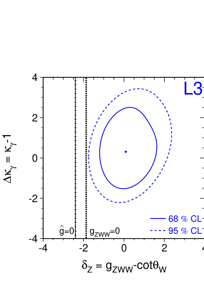
Figure 8: Bounds on $\Delta\kappa_{\gamma}\equiv X_{\gamma}$ and $\delta_{Z}$ obtained [43] by the L3 Collaboration at LEP.

Figs. 7a and 7b from Ref. [43] are based on the assumption that future data on $e^{+}e^{-}\rightarrow W^{+}W^{-}$ at an energy of 175 GeV will agree with SM predictions within errors. Under this assumption, fig. 7a shows that an integrated luminosity of $8pb^{-1}$, corresponding to a few weeks of running at $175\,\mathrm{GeV}$ will be sufficient to provide direct experimental evidence for the existence of a non-vanishing coupling of the non-Abelian type, $\hat{g}\not=0$, among the members of the vector-boson triplet (at 95% C.L.). Likewise, according to fig. 7b, an integrated luminosity of $100pb^{-1}$, corresponding to about seven months of running at LEP2, will provide direct experimental evidence for a non-vanishing anomalous magnetic moment of the W boson (at 95% C.L.), $\kappa_{\gamma}\not=0$.

Figure 8 finally shows the experimental result [44] recently obtained by the L3 collaboration. The data at 95 % C.L. indeed rule out a vanishing weak (trilinear) coupling, $\hat{g}$, among the members of the $W^{0},W^{\pm}$ triplet as well as a vanishing of the $ZW^{+}W^{-}$ coupling, $g_{ZW^{+}W^{-}}$.

3 Conclusions

Let me conclude as follows:

• The Z data and the W-mass measurements require electroweak corrections beyond fermion-loop contributions to the vector-boson propagators.

• In the Standard Model such corrections are provided by bosonic loops. The dominant bosonic correction needed for agreement with the data can be traced back to the difference in scale between $\mu$ decay, entering via $G_{\mu}$, and W or Z decay. While not being sensitive to the Higgs mechanism, these bosonic corrections depend on the non-Abelian couplings among the vector bosons. The data accordingly “see” the non-Abelian structure of the Standard Model.

• The bounds on the mass, $M_{\mathrm{H}}$, of the Higgs scalar are most reliably derived from the reduced set of data containing $\bar{s}_{\scriptscriptstyle{\mathrm{W}}}^{2},M_{\mathrm{W}},\Gamma_{\mathrm{l}},m_{\mathrm{t}}^{{\rm exp}}$ and $\alpha(M_{\mathrm{Z}}^{2})$ besides $M_{\mathrm{Z}}$ and $G_{\mu}$. At 95% C.L. the 1996 set of data implies $M_{\mathrm{H}}\>\raisebox{-2.15277pt}{$\stackrel{{\scriptstyle\textstyle<}}{{\sim}}$}\>550$ GeV and $M_{\mathrm{H}}\>\raisebox{-2.15277pt}{$\stackrel{{\scriptstyle\textstyle<}}{{\sim}}$}\>800$ GeV, depending on whether $\bar{s}_{\scriptscriptstyle{\mathrm{W}}}^{2}$(LEP+SLD) or $\bar{s}_{\scriptscriptstyle{\mathrm{W}}}^{2}$(LEP) is used as input. The ‘97 data improve these bounds to $M_{H}\>\raisebox{-2.15277pt}{$\stackrel{{\scriptstyle\textstyle<}}{{\sim}}$}\>430\,\mathrm{GeV}$ and $M_{H}\>\raisebox{-2.15277pt}{$\stackrel{{\scriptstyle\textstyle<}}{{\sim}}$}\>680\,\mathrm{GeV}$, respectively. These bounds are quite remarkable, as for the first time they seem to fairly reliably predict a Higgs mass in the perturbative region of the SM.

• Since the “$R_{\mathrm{b}}$-crisis” has meanwhile been resolved by our experimental collegues, there is now perfect overall agreement with the predictions of the SM, even upon including hadronic $Z$ decays in the analysis. The strong coupling, $\alpha_{\mathrm{s}}(M_{\mathrm{Z}}^{2})$, obtainable from the hadronic Z-decay modes, comes out consistently with the event-shape analysis. Various speculations on “hadrophilic” or “leptophobic” bosons do not seem to be realized in nature.

• The experiments at LEP2 on $e^{+}e^{-}\rightarrow W^{+}W^{-}$ show direct experimental evidence for the existence of non-vanishing couplings of non-Abelian type among the vector bosons.

• The available data by themselves do not discriminate a MVB from the Standard Theory based on the Higgs mechanism. The issue of mass generation will remain open until the Higgs scalar will be found - or something else?

Acknowledgement
It is a pleasure to thank Misha Bilenky, Stefan Dittmaier, Carsten Grosse-Knetter, Karol Kolodziej, Masaaki Kuroda, Ingolf Kuss and Georg Weiglein for a fruitful collaboration on various aspects on the theory of electroweak interactions.

References

• [1]
• [2] R.P. Feynman in Theory of Fundamental Processes (Benjamin, New York 1962), p. VII.
• [3] S.L. Glashow, Nucl. Phys. B22 (1961) 579.
• [4] S. Weinberg, Phys. Rev. Lett. 19 (1967) 1264;
A. Salam, in Elementary Particle Theory, ed. N. Svartholm (Almqvist and Wiksell, Stockholm, 1968), p.367.
• [5] The LEP Electroweak Working Group and the SLD Heavy Flavour Group, Data presented at the 1996 Summer Conferences, LEPEWWG/96-02;
Data presented at the 1997 Summer Conferences, LEPEWWG/97-02;
G. Quast, invited talk at the Jerusalem Conference on High-Energy Physics, HEP ‘97, August ‘97.
• [6] SLD Collaboration: K. Abe et al., Phys. Rev. Lett. 73 (1994) 25;
SLD Collaboration: K. Abe et al., contributed paper to EPS-HEP-95, Brussels, eps0654.
• [7] UA2 Collaboration: J. Alitti et al., Phys. Lett. B276 (1992) 354;
CDF Collaboration: F. Abe et al., Phys. Rev. Lett. 65 (1990) 2243, Phys. Rev. D43 (1991) 2070, Phys. Rev. D52 (1995) 4784, Phys. Rev. Lett. 75 (1995) 11;
DØ Collaboration: S. Abachi et al., preliminary result presented by U. Heintz, Les Rencontres de Physique de la Vallee d’Aoste, La Thuile, March 1996.
• [8] H. Burkhardt and B. Pietrzyk, Phys. Lett. B356 (1995) 398;
S. Eidelman and F. Jegerlehner, Z. Phys. C67 (1995) 585.
• [9] S. Bethke, Proceedings of the QCD ’94 Conference, Montpellier, France, Nucl. Phys. B (Proc. Suppl.) 39B,C (1995) 198.
• [10] CDF Collaboration, F. Abe et al., contributed paper to ICHEP96, PA-08-018;
DØ Collaboration, S. Abachi et al., contributed papers to ICHEP96, PA-05-027 and PA-05-028;
P. Grannis, talk presented at 28th International Conference on High-energy Physics (ICHEP96) Warsaw, Poland, 1996.
• [11] G. Gounaris and D. Schildknecht, Z. Phys. C40 (1988) 447, C42 (1989) 107.
• [12] J.-L. Kneur, M. Kuroda and D. Schildknecht, Phys. Lett. B262 (1991) 93.
• [13] M. Bilenky, K. Kolodziej, M. Kuroda and D. Schildknecht, Phys. Lett. B319 (1993) 319.
• [14] S. Dittmaier, K. Kolodziej, M. Kuroda and D. Schildknecht, Nucl. Phys. B426 (1994) 249, E: B446 (1995) 334.
• [15] S. Dittmaier, M. Kuroda and D. Schildknecht, Nucl. Phys. B448 (1995) 3.
• [16] S. Dittmaier, D. Schildknecht and G. Weiglein, Nucl. Phys. B465 (1996) 3.
• [17] G. t’Hooft, Nucl. Phys. B35 (1971) 167,
B. W. Lee and J. Zinn-Justin, Phys. Rev. D5 (1971) 3121,
G. t’Hooft and M. Veltman, Nucl. Phys. B50 (1972) 318.
• [18] H. Burkhardt, F. Jegerlehner, G. Penso and C. Verzegnassi, Z. Phys. C43 (1989) 497.
• [19] V.A. Novikov, L. Okun and M.I. Vysotskii, Nucl. Phys. B397 (1993) 35,
V.A. Novikov, L.B. Okun, A.N. Rozanov and M.I. Vysotsky, Mod. Phys. Lett. A9 (1994) 2641.
• [20] D. Schildknecht, Acta Physica Polonica 25 (1994) 1337.
• [21] P.Q. Hung and J.J. Sakurai, Nucl. Phys. B143 (1978) 81;
J.D. Bjorken, Phys. Rev. D19 (1979) 335.
• [22] G. Altarelli, B. Barbieri and F. Caravaglios, Nucl. Phys. B405 (1993) 3; Phys. Lett. B349 (1995) 145.
• [23] S. Dittmaier and D. Schildknecht, Phys. Lett. B391 (1997) 420.
• [24] M. Veltman, Nucl. Phys. B123 (1977) 89.
• [25] The LEP Electroweak Working Group and the SLD Heavy Flavour Group, Data presented at the 1995 Summer Conferences, LEPEWWG/95-02.
• [26] M. Kuroda, I. Kuss and D. Schildknecht, hep-ph/9705294, Phys. Lett. B409 (1997) 405.
• [27] P.W. Higgs, Phys. Rev. 145 (1966) 1156;
T.W. Kibble, Phys. Rev. 155 (1967) 1554.
• [28] S. Dittmaier, C. Grosse-Knetter and D. Schildknecht, Z. Phys. C67 (1995) 109.
• [29] E.C.G. Stueckelberg, Helv. Phys. Acta 11 (1938), 129;
Helv. Phys. Acta 30 (1956) 209.
• [30] T. Kunimasa and T. Goto, Progr. Theor. Phys. 37 (1967) 452;
T. Sonoda and S.Y. Tsai, Prog. Theor. Phys. 71 (1984) 878;
C. Grosse-Knetter and R. Kögerler, Phys. Rev. D48 (1993) 2865.
• [31] M.J. Herrero and E. Ruiz Morales, Nucl. Phys. B418 (1994) 431;
S. Dittmaier and C. Grosse-Knetter, Nucl. Phys. B459 (1996) 497.
• [32] S. Dittmaier, D. Schildknecht and G. Weiglein, Phys. Lett. B386 (1996) 247; see also hep-ph/9605268, Proceedings of the XXXIth RECONTRES DE MORIOND, “Electroweak interactions and unified theories”, ed. J. Trân Thanh Vân, Les Arcs, Savoie, France, March 9-16, 1996, p. 135.
• [33] W. de Boer, A. Dabelstein, W. Hollik, W. Mösle and U. Schwickerath, IEKP-KA/96-08, KA-TP-18-96, hep-ph/9609209;
J. Ellis, G.L. Fogli and E. Lisi, Phys. Lett. B389 (1996) 321.
• [34] G. Montagna, O. Nicrosini, G. Passarino and F. Piccinini, Phys. Lett. B335 (1994) 484;
V.A. Novikov, L.B. Okun, A.N. Rozanov and M.I. Vysotskii, Mod. Phys. Lett. A9 (1994) 2641;
J. Erler and P. Langacker, Phys. Rev. D52 (1995) 441;
S. Matsumoto, Mod. Phys. Lett. A10 (1995) 2553;
Z. Hioki, Acta Phys. Polon. B27 (1996) 2573;
K. Kang and S.K. Kang, BROWN-HET-979, hep-ph/9503478, Proceedings BEYOND THE STANDARD MODEL IV, 605, Tahoe City 1994, USA;
G. Passarino, hep-ph/9604344.
• [35] J. Ellis, G.L. Fogli and E. Lisi, Z. Phys. C69 (1996) 627;
P.H. Chankowski and S. Pokorski, Phys. Lett. B356 (1995) 307; hep-ph/9509207.
• [36] P. Chiappetta, J. Layssac, F.M. Renard and C. Verzegnassi, Phys. Rev. D54 (1996) 789.
• [37] G. Altarelli, N. di Bartholomeo, F. Feruglio, R. Gatto and M.L. Mangano, Phys. Lett. B375 (1996) 292.
• [38] P.H. Framption, M.B. Wise and B.D. Wright, Phys. Rev. D54 (1996) 5820.
• [39] J.J. Sakurai, in High-Energy Physics with Polarized Beams and Polarized Targets, Argonne 1978, AIP Conference Proceedings, No. 51 (1979), ed. G.H. Thomas, p. 138.
• [40] M. Bilenky, J. L. Kneur, F. M. Renard and D. Schildknecht, Nucl. Phys. B409 (1993) 22, B419 (1994) 240.
• [41] C. Grosse-Knetter, I. Kuss and D. Schildknecht, Phys. Lett. B358 (1995) 87.
• [42] J. Maalampi, D. Schildknecht and K.H. Schwarzer, Phys. Lett. B166 (1986) 361; M. Kuroda, J. Maalampi, D. Schildknecht and K.H. Schwarzer, Nucl. Phys. B284 (1987) 271; Phys. Lett. B190 (1987) 217.
• [43] I. Kuss and D. Schildknecht, Phys. Lett. B383 (1996) 470.
• [44] L3 Collaboration, M. Acciarri et al. CERN-PPE/97-98 to appear in Phys. Lett. B.