CERN-TH/97-313

SHEP–97/23

FTUV/97–47

IFIC/97–78

hep-ph/9711307

Radiative Corrections to Chargino Production in Electron-Positron Collisions

Marco A. Díaz¹, Steve F. King^2∗, and Douglas A. Ross³

¹ Departamento de Física Teórica, IFIC–CSIC, Universidad de Valencia
Burjassot, Valencia 46100, Spain
² CERN, Theory Division, CH–1211 Geneva, Switzerland
³ Department of Physics and Astronomy, University of Southampton
Southampton, SO17 1BJ, U.K.

Abstract

We discuss the one-loop radiative corrections to the reaction $\sigma(e^{+}e^{-}\rightarrow\tilde{\chi}^{+}_{a}\tilde{\chi}^{-}_{b})$, for $a,b=1,2$ where $\tilde{\chi}^{\pm}_{1,2}$ are the charginos of the minimal supersymmetric standard model. We calculate the leading one loop radiative corrections involving loops of top, stop, bottom and sbottom quarks, working in the $\overline{MS}$ scheme. At LEP2 we find positive radiative corrections typically of $10\%$ to $15\%$ and with a maximum value of approximately $30\%$ if the squark mass parameters are of the order of 1 TeV. If $\sqrt{s}=500$ GeV we find smaller corrections but they can be also negative, with extreme values of $13\%$ and $-4\%$. For a center of mass given by $\sqrt{s}=2$ TeV we find larger corrections, with typical values between $20\%$ and $-20\%$.

CERN-TH/97-313

^∗ On leave of absence from ³.

1 Introduction

The $e^{+}e^{-}$ colliders such as LEP provide a clean environment for searching for the charginos and neutralinos predicted by the minimal supersymmetric standard model (MSSM) [1]. Several authors have considered the production of neutralinos and charginos at $e^{+}e^{-}$ colliders at the $Z$ pole [2] and beyond [3], as well as its decay modes [4]. From an accurate measurement of the chargino production cross-section, much information could be obtained about the MSSM [5, 6].

Experimental searches for charginos at LEP2 have been negative so far, and lower bounds on the lightest chargino mass have been set. The bound depends mainly on the sneutrino mass and the mass difference between the chargino and the LSP $\Delta m=m_{\chi_{1}}-m_{\chi^{0}_{1}}$. ALEPH has found that $m_{\chi_{1}}>85$ GeV for $m_{\tilde{\nu}_{e}}>200$ GeV [7]. DELPHI’s bound corresponds to $m_{\chi_{1}}>84.3$ GeV for $m_{\tilde{\nu}_{e}}>300$ GeV and $\Delta m>10$ GeV [8]. A lower bound of $m_{\chi_{1}}>85.5$ GeV was found by L3 for $m_{\tilde{\nu}_{e}}>300$ GeV [9]. Finally, OPAL has found that if $\Delta m>10$ GeV then $m_{\chi_{1}}>84.5$ GeV if $m_{0}>1$ TeV and $m_{\chi_{1}}>65.7$ GeV for the smallest $m_{0}$ compatible with current limits on sneutrino and slepton masses [10].

Given the importance of an accurate measurement of the chargino production cross-section in $e^{+}e^{-}$ experiments, it is clearly important to be able to calculate this cross-section as accurately as possible. Although this cross-section does not contain any coloured particles, and so is immune to QCD corrections, there are other radiative corrections which, as we shall see, may give large corrections to the cross-section of order 10%. Although electroweak corrections may be expected to give corrections of order 1%, there are additional radiative corrections coming from loops of top and bottom quarks and squarks which are important due to the large Yukawa couplings of these heavy quarks and squarks, and it is these corrections which form the subject of the present paper. Although radiative corrections to chargino masses have been considered [11], the radiative corrections to chargino production in $e^{+}e^{-}$ experiments has not so been considered in the literature.

The layout of this paper is as follows. In Section 2 we discuss the tree level amplitude and outline the approach to radiative corrections which we follow. In Section 3 we introduce convenient form factors which enable the calculation to be organized in terms of its possible Lorentz invariant structures, and express the square of the amplitude in terms of the form factors. In section 4 we describe how the different diagrams contribute to the form factors, relegating many of the details to a series of Appendices where the Feynman rules and Passarino–Veltman (PV) functions are also summarised. Section 5 contains the numerical results, and in Section 6 we give our conclusions.

2 Tree Level Amplitude and Its One–Loop Renormalization

We consider the pair production of charginos with momenta $k_{1}$ and $k_{2}$ in electron-positron scattering with incoming momenta $p_{1}$ and $p_{2}$:

$$e^{+}(p_{2})+e^{-}(p_{1})\rightarrow\tilde{\chi}^{+}_{b}(k_{2})+\tilde{\chi}^{-}_{a}(k_{1})$$ (2.1)

In the MSSM charginos can be produced in the s–channel with intermediate $Z$–bosons and photons, and in the t–channel with an intermediate electron–type sneutrino. We denote these amplitudes $M_{Z}^{0}$, $M_{\gamma}^{0}$, and $M_{\tilde{\nu}}^{0}$, where the superscript 0 indicates that the amplitude is at tree level. These amplitudes correspond to the diagrams in Fig. 1 with the shaded blobs replaced by the lowest order tree-level vertices.

The tree level $Z$ amplitude can be written as

$$M_{Z}^{0}=\Big{[}\overline{v}(p_{2})i{\cal G}_{Zee}^{0,\mu}u(p_{1})\Big{]}P_{Z}^{\mu\nu}(p^{2})\Big{[}\overline{u}(k_{2})i{\cal G}_{Z\chi\chi}^{0,ab\nu}v(k_{1})\Big{]}$$ (2.2)

where

$$P_{Z}^{\mu\nu}(p^{2})={{-ig^{\mu\nu}}\over{p^{2}-m_{Z}^{2}-im_{Z}\Gamma_{Z}}}$$ (2.3)

is the $Z$–boson propagator in the Feynman gauge, with $m_{Z}$ its mass, $\Gamma_{Z}$ its total width, and $p^{2}=(p_{1}+p_{2})^{2}=(k_{1}+k_{2})^{2}=s$ is the square of the center of mass energy. The tree level $Ze^{+}e^{-}$ vertex function is

$${\cal G}_{Zee}^{0,\mu}=-{g\over{2c_{W}}}\gamma^{\mu}(g_{V}^{e}-g_{A}^{e}\gamma_{5})$$ (2.4)

where $g$ is the $SU(2)$ gauge coupling, $s_{W}=\sin\theta_{W}$, $c_{W}=\cos\theta_{W}$ where $\theta_{W}$ is the weak angle, and $g_{V}^{e}=-1/2+2s_{W}^{2}$ and $g_{A}^{e}=-1/2$.

Similarly, the $Z\tilde{\chi}^{+}_{b}\tilde{\chi}^{-}_{a}$ vertices are given by

$${\cal G}_{Z\chi\chi}^{0,ab\nu}={g\over{2c_{W}}}\gamma^{\nu}\Big{[}O^{\prime L}_{ab}(1-\gamma_{5})+O^{\prime R}_{ab}(1+\gamma_{5})\Big{]}$$ (2.5)

where the couplings $O^{\prime L}_{ab}$ and $O^{\prime R}_{ab}$ are related to the matrices which diagonalize the chargino mass matrix, and are defined in Appendix A.

The tree level photon amplitude can be written as

$$M_{\gamma}^{0}=\Big{[}\overline{v}(p_{2})i{\cal G}_{\gamma ee}^{0,\mu}u(p_{1})\Big{]}P_{\gamma}^{\mu\nu}(p^{2})\Big{[}\overline{u}(k_{2})i{\cal G}_{\gamma\chi\chi}^{0,ab\nu}v(k_{1})\Big{]}$$ (2.6)

where the photon propagator in the Feynman gauge is

$$P_{\gamma}^{\mu\nu}(p^{2})={{-ig^{\mu\nu}}\over{p^{2}}}$$ (2.7)

The photon tree level vertices are very simple:

$${\cal G}_{\gamma ee}^{0,\mu}=e\gamma^{\mu}\,,\qquad{\cal G}_{\gamma\chi\chi}^{0,ab\nu}=-e\gamma^{\nu}\delta_{ab}$$ (2.8)

where $e=|e|$ and the factor of $q_{e}=-1$ for the electron charge has been used.

Finally, the tree level sneutrino amplitude is

$$M_{\tilde{\nu}}^{0}=\Big{[}\overline{v}(p_{2})i{\cal G}_{\tilde{\nu}_{e}e\chi}^{0,+b}\overline{u}^{T}(k_{2})\Big{]}P_{\tilde{\nu}_{e}}(q^{2})\Big{[}v^{T}(k_{1})i{\cal G}_{\tilde{\nu}_{e}e\chi}^{0,-a}u(p_{1})\Big{]}$$ (2.9)

where

$$P_{\tilde{\nu}_{e}}(q^{2})={i\over{q^{2}-m_{\tilde{\nu}_{e}}^{2}}}$$ (2.10)

is the sneutrino propagator, $m_{\tilde{\nu}_{e}}$ is its mass and $q^{2}=(k_{2}-p_{2})^{2}=(p_{1}-k_{1})^{2}=t$ is the squared of the t–channel momentum transferred. The sneutrino vertices are at tree level given by

$${\cal G}_{\tilde{\nu}_{e}e\chi}^{0,+b}=-{g\over 2}V_{b1}(1+\gamma_{5})C\,,\qquad{\cal G}_{\tilde{\nu}_{e}e\chi}^{0,-a}={g\over 2}C^{-1}V_{a1}^{*}(1-\gamma_{5})$$ (2.11)

Here, $C$ is the charge conjugation matrix and $V$ is one of the diagonalization matrices of the chargino mass matrix (see Appendix A).

Divergent diagrams are regularized using dimensional regularization. Therefore, the divergences are contained in the parameter

$$\Delta={2\over{4-n}}+\ln 4\pi-\gamma_{E},$$ (2.12)

where $n$ is the number of space–time dimensions, and $\gamma_{E}$ is the Euler’s constant. In every divergent graph, the term $\Delta$ is always accompanied by the term $\ln Q^{2}$, where $Q$ is an arbitrary mass scale introduced by dimensional regularization. The renormalization scheme we use here is the $\overline{MS}$. In this scheme, the counterterm is fixed in such a way that cancels only the terms proportional to $\Delta$. As a consequence, one–loop corrections (diagrams plus counterterms) to 1PI Green’s functions become finite but remain scale dependent. In order to get a physical scattering amplitude, i.e., independent of the scale $Q$, the tree level parameters are promoted to running parameters. This implicit scale dependence of the tree level parameters cancels the explicit scale dependence of the one–loop corrections to the scattering amplitude.

We work in the approximation where only top and bottom quarks and squarks are considered in the loops. These corrections are in general enhanced by logarithms of large mass ratios and by Yukawa couplings, whereas other corrections are genuinely of order $\alpha_{W}$ and therefore negligible. This implies, for example, that the electron–positron vertices, ${\cal G}_{Zee}^{\mu}$ and ${\cal G}_{\gamma ee}^{\mu}$, do not receive triangular corrections, and the tree level vertex can be identify with the one–loop renormalized vertex. In the following section we detail all these one–loop corrections to the chargino pair production.

3 Squared Amplitudes in Terms of Form Factors

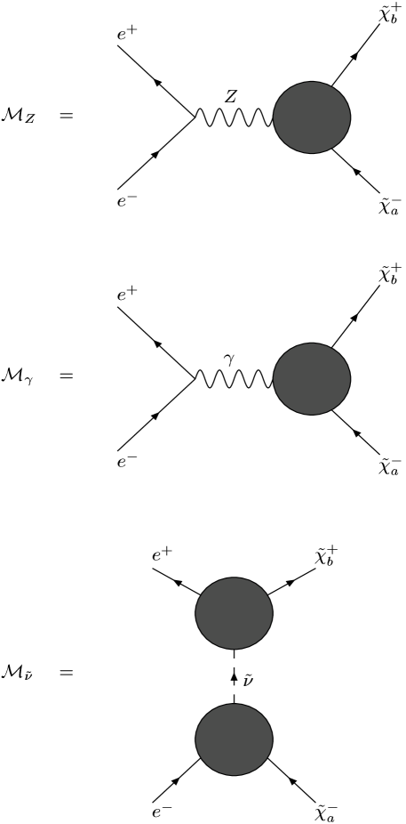
Figure 1: One–loop renormalized $M_{Z}$, $M_{\gamma}$ and $M_{\tilde{\nu}_{e}}$ amplitudes in the approximation where only top and bottom quarks and squarks are considered inside the loops.

In the presence of radiative corrections, the amplitude for $e^{+}e^{-}\rightarrow\tilde{\chi}^{+}_{b}\tilde{\chi}^{-}_{a}$ may be expressed as the sum of three amplitudes $M_{Z}$, $M_{\gamma}$, $M_{\tilde{\nu}}$ as shown in Fig. 1. The shaded bubbles in that figure are one–loop renormalized total vertex functions defined as $i{\cal G}_{Z\chi\chi}^{ab}$, $i{\cal G}_{\gamma\chi\chi}^{ab}$, $i{\cal G}_{\tilde{\nu_{e}}e\chi}^{+b}$, and $i{\cal G}_{\tilde{\nu_{e}}e\chi}^{-a}$. In the total vertex functions we include the tree level vertex, the one–particle irreducible vertex diagrams plus the vertex counterterm, and the one–particle reducible vertex diagrams plus their counterterms. Although the detailed expressions for the total vertex functions is quite complicated, by exploiting the possible Lorentz structures of the diagrams it is possible to express them in terms of just a few form factors.

We define the Z form factors as follows:

$${\cal G}_{Z\chi\chi}^{ab}\equiv(1+\gamma_{5})\left(F_{Z0}^{+}\gamma^{\mu}+F_{Z1}^{+}k_{1}^{\mu}+F_{Z2}^{+}k_{2}^{\mu}\right)+(1-\gamma_{5})\left(F_{Z0}^{-}\gamma^{\mu}+F_{Z1}^{-}k_{1}^{\mu}+F_{Z2}^{-}k_{2}^{\mu}\right)$$ (3.1)

Similarly we define the photon form factors as follows:

$${\cal G}_{\gamma\chi\chi}^{ab}\equiv(1+\gamma_{5})\left(F_{\gamma 0}^{+}\gamma^{\mu}+F_{\gamma 1}^{+}k_{1}^{\mu}+F_{\gamma 2}^{+}k_{2}^{\mu}\right)+(1-\gamma_{5})\left(F_{\gamma 0}^{-}\gamma^{\mu}+F_{\gamma 1}^{-}k_{1}^{\mu}+F_{\gamma 2}^{-}k_{2}^{\mu}\right)$$ (3.2)

Sneutrino total vertex functions are simpler. There are two total sneutrino vertex functions denoted by ${\cal G}_{\tilde{\nu_{e}}e\chi}^{\pm a}$, and each of them can be express in terms of a single form factor. For the upper vertex we have:

$${\cal G}_{\tilde{\nu_{e}}e\chi}^{+b}\equiv(1+\gamma_{5})CF_{\tilde{\nu_{e}}}^{+}$$ (3.3)

For the lower vertex we have:

$${\cal G}_{\tilde{\nu_{e}}e\chi}^{-a}\equiv C^{-1}(1-\gamma_{5})F_{\tilde{\nu_{e}}}^{-}$$ (3.4)

Having expressed the vertices $Z\chi_{b}^{+}\chi_{a}^{-}$, $\gamma\chi_{b}^{+}\chi_{a}^{-}$, $\tilde{\nu}e^{+}\chi_{b}^{+}$, and $\tilde{\nu}e^{-}\chi_{a}^{-}$ in terms of form factors, it is a relatively straightforward task to write down the one-loop amplitudes in terms of the form factors.

The $Z$ amplitude squared is

$$\langle|M_{Z}|^{2}\rangle = {{g^{2}}\over{c_{W}^{2}}}{{s^{2}}\over{(s-m_{Z}^{2})^{2}+m_{Z}^{2}\Gamma_{Z}^{2}}}\Bigg{\{}$$ (3.5)

$$2g_{V}^{e}g_{A}^{e}\left(|F_{Z0}^{-}|^{2}-|F_{Z0}^{+}|^{2}\right)R+\left(g_{V}^{e2}+g_{A}^{e2}\right)\bigg{\{}4m_{\chi_{a}}m_{\chi_{b}}{\mathrm{R}e}(F_{Z0}^{+}F_{Z0}^{-*})/s$$

$$+{\textstyle{1\over 2}}\left(|F_{Z0}^{+}|^{2}+|F_{Z0}^{-}|^{2}\right)\left[1+R^{2}-(m_{\chi_{a}}^{2}-m_{\chi_{b}}^{2})^{2}/s^{2}\right]$$

$$+{\textstyle{1\over 2}}\bigg{[}{\mathrm{R}e}\left[(m_{\chi_{a}}F_{Z0}^{-}+m_{\chi_{b}}F_{Z0}^{+})(F_{Z1}^{-}-F_{Z2}^{-})^{*}\right]$$

$$\qquad+{\mathrm{R}e}\left[(m_{\chi_{a}}F_{Z0}^{+}+m_{\chi_{b}}F_{Z0}^{-})(F_{Z1}^{+}-F_{Z2}^{+})^{*}\right]$$

$$\qquad+{\textstyle{1\over 4}}(s-m_{\chi_{a}}^{2}-m_{\chi_{b}}^{2})\left(|F_{Z1}^{-}-F_{Z2}^{-}|^{2}+|F_{Z1}^{+}-F_{Z2}^{+}|^{2}\right)$$

$$\qquad-m_{\chi_{a}}m_{\chi_{b}}{\mathrm{R}e}\left[(F_{Z1}^{-}-F_{Z2}^{-})(F_{Z1}^{+}-F_{Z2}^{+})^{*}\right]$$

$$\!\!\qquad\bigg{]}\left[1-R^{2}-2(m_{\chi_{a}}^{2}+m_{\chi_{b}}^{2})/s+(m_{\chi_{a}}^{2}-m_{\chi_{b}}^{2})^{2}/s^{2}\right]\bigg{\}}\Bigg{\}}$$

where

$$R=\lambda^{1/2}(1,m_{\chi_{a}}^{2}/s,m_{\chi_{b}}^{2}/s)\cos\theta\,,$$ (3.6)

$\lambda(a,b,c)=(a+b-c)^{2}-4ab$, and $\theta$ is the angle between the electron and chargino lines. Note that we have already sum over final spin configurations and taken the average of initial spin configurations. The photon amplitude squared is given by

$$\langle|M_{\gamma}|^{2}\rangle = 2e^{2}\Bigg{\{}8m_{\chi_{a}}m_{\chi_{b}}{\mathrm{R}e}(F_{\gamma 0}^{+}F_{\gamma 0}^{-*})/s$$ (3.7)

$$+\left(|F_{\gamma 0}^{+}|^{2}+|F_{\gamma 0}^{-}|^{2}\right)\left[1+R^{2}-(m_{\chi_{a}}^{2}-m_{\chi_{b}}^{2})^{2}/s^{2}\right]$$

$$+\bigg{[}{\mathrm{R}e}\left[(m_{\chi_{a}}F_{\gamma 0}^{-}+m_{\chi_{b}}F_{\gamma 0}^{+})(F_{\gamma 1}^{-}-F_{\gamma 2}^{-})^{*}\right]$$

$$\qquad+{\mathrm{R}e}\left[(m_{\chi_{a}}F_{\gamma 0}^{+}+m_{\chi_{b}}F_{\gamma 0}^{-})(F_{\gamma 1}^{+}-F_{\gamma 2}^{+})^{*}\right]$$

$$\qquad+{\textstyle{1\over 4}}(s-m_{\chi_{a}}^{2}-m_{\chi_{b}}^{2})\left(|F_{\gamma 1}^{-}-F_{\gamma 2}^{-}|^{2}+|F_{\gamma 1}^{+}-F_{\gamma 2}^{+}|^{2}\right)$$

$$\qquad-m_{\chi_{a}}m_{\chi_{b}}{\mathrm{R}e}\left[(F_{\gamma 1}^{-}-F_{\gamma 2}^{-})(F_{\gamma 1}^{+}-F_{\gamma 2}^{+})^{*}\right]$$

$$\quad\bigg{]}\left[1-R^{2}-2(m_{\chi_{a}}^{2}+m_{\chi_{b}}^{2})/s+(m_{\chi_{a}}^{2}-m_{\chi_{b}}^{2})^{2}/s^{2}\right]\Bigg{\}}$$

and the sneutrino amplitude squared is

$$\langle|M_{\tilde{\nu}_{e}}|^{2}\rangle=|F_{\tilde{\nu}_{e}}^{+}|^{2}|F_{\tilde{\nu}_{e}}^{-}|^{2}{{s^{2}}\over{(t-m_{\tilde{\nu}_{e}}^{2})^{2}}}\left[(1-R)^{2}-(m_{\chi_{a}}^{2}-m_{\chi_{b}}^{2})^{2}/s^{2}\right]$$ (3.8)

The total amplitude squared has three interferences. We start with the $Z$–photon interference

$$2{\mathrm{R}e}\langle M_{Z}M_{\gamma}^{*}\rangle\;\>=\;\>{{eg}\over{c_{W}}}{\mathrm{R}e}{s\over{s-m_{Z}^{2}-im_{Z}\Gamma_{Z}}}\Bigg{\{}4g_{A}^{e}(F_{Z0}^{-}F_{\gamma 0}^{-*}-F_{Z0}^{+}F_{\gamma 0}^{+*})+g_{V}^{e}\bigg{\{}$$

$$\qquad\;8m_{\chi_{a}}m_{\chi_{b}}(F_{Z0}^{+}F_{\gamma 0}^{-*}+F_{Z0}^{-}F_{\gamma 0}^{+*})/s$$

$$\qquad+2(F_{Z0}^{+}F_{\gamma 0}^{+*}+F_{Z0}^{-}F_{\gamma 0}^{-*})\left[1+R^{2}-(m_{\chi_{a}}^{2}-m_{\chi_{b}}^{2})^{2}/s^{2}\right]$$

$$\qquad+\bigg{[}(m_{\chi_{a}}F_{Z0}^{-}+m_{\chi_{b}}F_{Z0}^{-})(F_{\gamma 1}^{-}-F_{\gamma 2}^{-})^{*}+(m_{\chi_{a}}F_{Z0}^{+}+m_{\chi_{b}}F_{Z0}^{-})(F_{\gamma 1}^{+}-F_{\gamma 2}^{+})^{*}$$

$$\qquad\quad+(F_{Z1}^{-}-F_{Z2}^{-})(m_{\chi_{a}}F_{\gamma 0}^{-*}+m_{\chi_{b}}F_{\gamma 0}^{+*})+(F_{Z1}^{+}-F_{Z2}^{+})(m_{\chi_{a}}F_{\gamma 0}^{+*}+m_{\chi_{b}}F_{\gamma 0}^{-*})$$

$$\qquad\quad+{\textstyle{1\over 2}}(s-m_{\chi_{a}}^{2}-m_{\chi_{b}}^{2})\left[(F_{Z1}^{-}-F_{Z2}^{-})(F_{\gamma 1}^{-}-F_{\gamma 2}^{-})^{*}+(F_{Z1}^{+}-F_{Z2}^{+})(F_{\gamma 1}^{+}-F_{\gamma 2}^{+})^{*}\right]$$

$$\qquad\quad-m_{\chi_{a}}m_{\chi_{b}}\left[(F_{Z1}^{-}-F_{Z2}^{-})(F_{\gamma 1}^{+}-F_{\gamma 2}^{+})^{*}+(F_{Z1}^{+}-F_{Z2}^{+})(F_{\gamma 1}^{-}-F_{\gamma 2}^{-})^{*}\right]$$

$$\qquad\quad\bigg{]}\left[1-R^{2}-2(m_{\chi_{a}}^{2}+m_{\chi_{b}}^{2})/s+(m_{\chi_{a}}^{2}-m_{\chi_{b}}^{2})^{2}/s^{2}\right]\bigg{\}}\Bigg{\}}$$ (3.9)

The $Z$-sneutrino interference is

$$2{\mathrm{R}e}\langle M_{Z}M_{\tilde{\nu}_{e}}^{*}\rangle = {{g(g_{V}^{e}+g_{A}^{e})}\over{c_{W}}}{\mathrm{R}e}{{s^{2}}\over{(s-m_{Z}^{2}-im_{Z}\Gamma_{Z})(t-m_{\tilde{\nu}_{e}}^{2})}}F_{\tilde{\nu_{e}}}^{+}F_{\tilde{\nu_{e}}}^{-}\bigg{\{}$$ (3.10)

$$4F_{Z0}^{-}m_{\chi_{a}}m_{\chi_{b}}/s+F_{Z0}^{+}\left[(1-R)^{2}-(m_{\chi_{a}}^{2}-m_{\chi_{b}}^{2})^{2}/s^{2}\right]$$

$$+{\textstyle{1\over 2}}\Big{[}m_{\chi_{a}}(F_{Z1}^{+}-F_{Z2}^{+})+m_{\chi_{b}}(F_{Z1}^{-}-F_{Z2}^{-})$$

$$\quad\;\,\Big{]}\left[1-R^{2}-2(m_{\chi_{a}}^{2}+m_{\chi_{b}}^{2})/s+(m_{\chi_{a}}^{2}-m_{\chi_{b}}^{2})^{2}/s^{2}\right]\bigg{\}}$$

and the photon–sneutrino interference is given by

$$2{\mathrm{R}e}\langle M_{\gamma}M_{\tilde{\nu}_{e}}^{*}\rangle = 2e{s\over{(t-m_{\tilde{\nu}_{e}}^{2})}}{\mathrm{R}e}\,F_{\tilde{\nu_{e}}}^{+}F_{\tilde{\nu_{e}}}^{-}\bigg{\{}$$ (3.11)

$$4F_{\gamma 0}^{-}m_{\chi_{a}}m_{\chi_{b}}/s+F_{\gamma 0}^{+}\left[(1-R)^{2}-(m_{\chi_{a}}^{2}-m_{\chi_{b}}^{2})^{2}/s^{2}\right]$$

$$+{\textstyle{1\over 2}}\Big{[}m_{\chi_{a}}(F_{\gamma 1}^{+}-F_{\gamma 2}^{+})+m_{\chi_{b}}(F_{\gamma 1}^{-}-F_{\gamma 2}^{-})$$

$$\quad\;\,\Big{]}\left[1-R^{2}-2(m_{\chi_{a}}^{2}+m_{\chi_{b}}^{2})/s+(m_{\chi_{a}}^{2}-m_{\chi_{b}}^{2})^{2}/s^{2}\right]\bigg{\}}$$

Now we just have to calculate the one–loop contributions to each form factor, and this is done in the next section.

4 Loop Contributions to Form Factors

In the previous section we defined the total vertex functions $i{\cal G}_{Z\chi\chi}^{ab}$, $i{\cal G}_{\gamma\chi\chi}^{ab}$, and ${\cal G}_{\tilde{\nu_{e}}e\chi}^{\pm a}$ expressed in terms of form factors $F_{Zi}^{\pm}$, $F_{\gamma i}^{\pm}$, with $i=0,1,2$, and $F_{\tilde{\nu}_{e}}^{\pm}$. In this section we give details about the contributions from the different diagrams to the form factors defined in the previous section. We divide the diagrams into one–particle irreducible triangular diagrams and one–particle reducible diagrams composed by gauge boson two–point functions, chargino mixing, and chargino wavefunction renormalization (see Appendix C).

The sum of the one-particle-irreducible vertex diagrams $i{\Gamma}_{Z\chi\chi}^{ab}$ includes one-loop triangle diagrams with internal top, bottom, stop, and sbottom quarks. Each of these graphs in terms of Passarino–Veltman (PV) functions [12] are given in Appendix C. From there one can read off the contribution of each graph to the form factors $F_{Zi}^{\pm}$, $i=0,1,2$, defined in eq. (3.1). This is particularly simple because the one-particle-irreducible vertex function $i{\Gamma}_{Z\chi\chi}^{ab}$ has the same Lorentz structure as the total vertex function $i{\cal G}_{Z\chi\chi}^{ab}$ in eq. (3.1). These contributions are graphically represented by the diagram in Fig. 2f, with an external $Z$-boson.

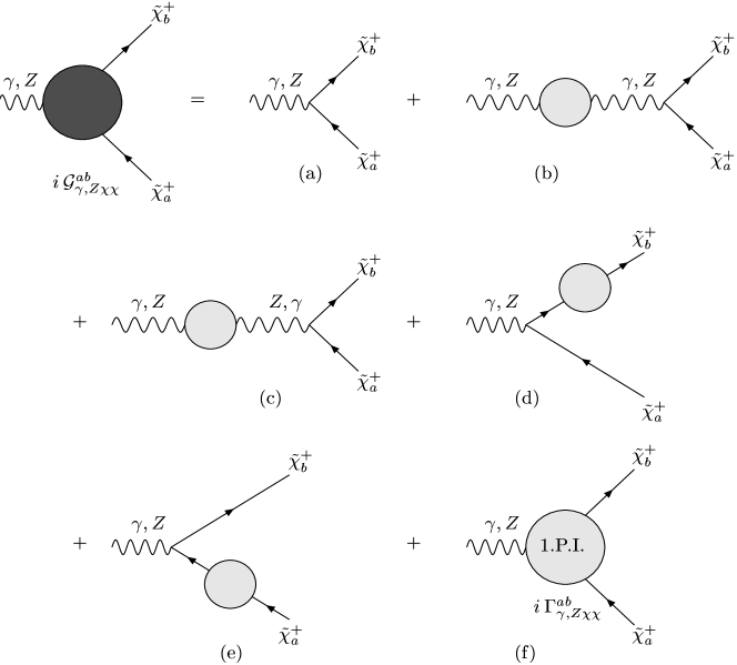
Figure 2: One–loop renormalized $\gamma\chi^{+}_{b}\chi^{-}_{a}$ and $Z\chi^{+}_{b}\chi^{-}_{a}$ vertex functions.

The sum of all one-particle-irreducible vertex diagrams $i{\Gamma}_{\gamma\chi\chi}^{ab}$ are treated in a completely analogous way. These graphs are also given in Appendix C, and from those expressions one can read off the corresponding contributions to the form factors $F_{\gamma i}^{\pm}$ in the total vertex function $i{\cal G}_{\gamma\chi\chi}^{ab}$. These contributions are also represented by the diagram in Fig. 2f, but with an external photon attached to it.

There are no contributions from triangular graphs to the form factors $F_{\tilde{\nu}_{e}}^{\pm}$ in the total vertex functions ${\cal G}_{\tilde{\nu_{e}}e\chi}^{\pm a}$. In the following subsections we analyse the one-particle-reducible graphs.

4.1 Gauge Bosons Two–Point Functions

The contribution from the gauge boson two–point functions is displayed in Fig. 2b and 2c. The general structure of the gauge boson two–point functions is

$$\Sigma_{GG}^{\mu\nu}(p^{2})=i[A_{GG}(p^{2})g^{\mu\nu}+B_{GG}(p^{2})p^{\mu}p^{\nu}]$$ (4.1)

where $p$ is the external momentum and $GG=ZZ$, $\gamma\gamma$, or $Z\gamma$. The functions $A_{GG}$ and $B_{GG}$ depend on the external momentum squared $p^{2}$ and represent the one–loop contributions to the gauge bosons self energies and mixing. For our purposes only $A_{GG}$ is relevant and these are displayed in Appendix C2. The gauge boson two–point functions attached to the external chargino line give contributions to the forms factors $F_{Z0}^{\pm}$ and $F_{\gamma 0}^{\pm}$ only.

The $Z$–boson self energy contributes to $F_{Z0}^{+}$ and $F_{Z0}^{-}$ form factors in the following way

$$F_{Z0}^{+}={g\over{2c_{W}}}O^{\prime L}_{ab}{{\widetilde{A}_{ZZ}(p^{2})}\over{p^{2}-m_{Z}^{2}}}\,,\qquad F_{Z0}^{-}={g\over{2c_{W}}}O^{\prime R}_{ab}{{\widetilde{A}_{ZZ}(p^{2})}\over{p^{2}-m_{Z}^{2}}}\,,$$ (4.2)

where $p^{2}=s$, the center–of–mass energy, and the tilde in $\widetilde{A}$ represent the self energy plus its counterterm, i.e., $\widetilde{A}$ is the finite two–point function.

Another contribution to the same form factors come from the $Z-\gamma$ mixing:

$$F_{Z0}^{+}=-{e\over 2}\delta_{ab}{{\widetilde{A}_{Z\gamma}(p^{2})}\over{p^{2}}}\,,\qquad F_{Z0}^{-}=-{e\over 2}\delta_{ab}{{\widetilde{A}_{Z\gamma}(p^{2})}\over{p^{2}}}\,,$$ (4.3)

where we take $e$ to be positive.

In a similar way, the $F_{\gamma 0}^{+}$ and $F_{\gamma 0}^{-}$ form factors receive the following contributions from the photon self energy

$$F_{\gamma 0}^{+}=-{e\over 2}\delta_{ab}{{\widetilde{A}_{\gamma\gamma}(p^{2})}\over{p^{2}}}\,,\qquad F_{\gamma 0}^{-}=-{e\over 2}\delta_{ab}{{\widetilde{A}_{\gamma\gamma}(p^{2})}\over{p^{2}}}\,,$$ (4.4)

and from the $\gamma-Z$ mixing

$$F_{\gamma 0}^{+}={g\over{2c_{W}}}O^{\prime L}_{ab}{{\widetilde{A}_{\gamma Z}(p^{2})}\over{p^{2}-m_{Z}^{2}}}\,,\qquad F_{\gamma 0}^{-}={g\over{2c_{W}}}O^{\prime R}_{ab}{{\widetilde{A}_{\gamma Z}(p^{2})}\over{p^{2}-m_{Z}^{2}}}\,.$$ (4.5)

There is no contribution from gauge two–point functions to the ${\cal G}_{\tilde{\nu_{e}}e\chi}^{\pm a}$ total vertex functions.

4.2 Chargino Mixing

Chargino mixing graphs contribute to the total vertices ${\cal G}_{\gamma\chi\chi}^{ab}$ and ${\cal G}_{Z\chi\chi}^{ab}$ through diagrams represented in Fig. 2d and 2e.

The most general expression for the chargino two–point functions at one–loop is

$$i\Sigma_{\chi\chi}^{ij}(p)=i\bigg{\{}\Big{[}A_{ij}^{+}(p^{2})(1+\gamma_{5})+A_{ij}^{-}(p^{2})(1-\gamma_{5})\Big{]}+\Big{[}B_{ij}^{+}(p^{2})(1+\gamma_{5})+B_{ij}^{-}(p^{2})(1-\gamma_{5})\Big{]}p_{\mu}\gamma^{\mu}\bigg{\}}$$ (4.6)

and the contribution to the functions $A_{ij}^{\pm}$ and $B_{ij}^{\pm}$ from the different loops are given in Appendix C. Chargino mixings contribute to the form factors when the loop is attached to an external chargino. We start with the $Z\chi^{+}_{b}\chi^{-}_{a}$ vertex. If the loop is attached to the external $\tilde{\chi}^{+}_{b}$ chargino, we find the following contributions

$$F_{Z0}^{+} = -{g\over{c_{W}}}O^{\prime L}_{ai}{1\over{m_{\chi_{b}}^{2}-m_{\chi_{i}}^{2}}}\Big{[}m_{\chi_{b}}\widetilde{A}_{ib}^{-}+m_{\chi_{i}}\widetilde{A}_{ib}^{+}+m_{\chi_{b}}(m_{\chi_{b}}\widetilde{B}_{ib}^{+}+m_{\chi_{i}}\widetilde{B}_{ib}^{-})\Big{]}$$

$$F_{Z0}^{-} = -{g\over{c_{W}}}O^{\prime R}_{ai}{1\over{m_{\chi_{b}}^{2}-m_{\chi_{i}}^{2}}}\Big{[}m_{\chi_{b}}\widetilde{A}_{ib}^{+}+m_{\chi_{i}}\widetilde{A}_{ib}^{-}+m_{\chi_{b}}(m_{\chi_{b}}\widetilde{B}_{ib}^{-}+m_{\chi_{i}}\widetilde{B}_{ib}^{+})\Big{]}$$ (4.7)

where $i\neq b$. All the functions $\widetilde{A}^{\pm}(k_{2}^{2})$ and $\widetilde{B}^{\pm}(k_{2}^{2})$ are evaluated at $k_{2}^{2}=m_{\chi_{b}}^{2}$, and the tilde means that the corresponding function is finite. If the one–loop graph is attached to the external $\tilde{\chi}^{-}_{a}$ chargino, then the contributions to the $F^{\pm}_{Z0}$ form factors are

$$F_{Z0}^{+} = -{g\over{c_{W}}}O^{\prime L}_{bi}{1\over{m_{\chi_{a}}^{2}-m_{\chi_{i}}^{2}}}\Big{[}m_{\chi_{a}}\widetilde{A}_{ai}^{+}+m_{\chi_{i}}\widetilde{A}_{ai}^{-}+m_{\chi_{a}}(m_{\chi_{a}}\widetilde{B}_{ai}^{+}+m_{\chi_{i}}\widetilde{B}_{ai}^{-})\Big{]}$$

$$F_{Z0}^{-} = -{g\over{c_{W}}}O^{\prime R}_{bi}{1\over{m_{\chi_{a}}^{2}-m_{\chi_{i}}^{2}}}\Big{[}m_{\chi_{a}}\widetilde{A}_{ai}^{-}+m_{\chi_{i}}\widetilde{A}_{ai}^{+}+m_{\chi_{a}}(m_{\chi_{a}}\widetilde{B}_{ai}^{-}+m_{\chi_{i}}\widetilde{B}_{ai}^{+})\Big{]}$$ (4.8)

where $i\neq a$ and all the functions $\widetilde{A}^{\pm}(k_{1}^{2})$ and $\widetilde{B}^{\pm}(k_{1}^{2})$ are evaluated at $k_{1}^{2}=m_{\chi_{a}}^{2}$.

In a similar way, we find the contributions to the form factors associated to the vertex $\gamma\chi^{+}_{b}\chi^{-}_{a}$. If the chargino mixing graph is attached to the external $\tilde{\chi}^{+}_{b}$ chargino, we find

$$F_{\gamma 0}^{+} = {e\over{m_{\chi_{b}}^{2}-m_{\chi_{a}}^{2}}}\Big{[}m_{\chi_{b}}\widetilde{A}_{ab}^{-}+m_{\chi_{a}}\widetilde{A}_{ab}^{+}+m_{\chi_{b}}(m_{\chi_{b}}\widetilde{B}_{ab}^{+}+m_{\chi_{a}}\widetilde{B}_{ab}^{-})\Big{]}$$

$$F_{\gamma 0}^{-} = {e\over{m_{\chi_{b}}^{2}-m_{\chi_{a}}^{2}}}\Big{[}m_{\chi_{b}}\widetilde{A}_{ab}^{+}+m_{\chi_{a}}\widetilde{A}_{ab}^{-}+m_{\chi_{b}}(m_{\chi_{b}}\widetilde{B}_{ab}^{-}+m_{\chi_{a}}\widetilde{B}_{ab}^{+})\Big{]}$$ (4.9)

where as before, all the functions $\widetilde{A}^{\pm}(k_{2}^{2})$ and $\widetilde{B}^{\pm}(k_{2}^{2})$ are evaluated at $k_{2}^{2}=m_{\chi_{b}}^{2}$. The difference with respect to the previous case is that here we need $a\neq b$, otherwise this contribution is absent.

If the one–loop graph is attached to the external $\tilde{\chi}^{-}_{a}$ chargino, we get

$$F_{\gamma 0}^{+} = {e\over{m_{\chi_{a}}^{2}-m_{\chi_{b}}^{2}}}\Big{[}m_{\chi_{a}}\widetilde{A}_{ab}^{+}+m_{\chi_{b}}\widetilde{A}_{ab}^{-}+m_{\chi_{a}}(m_{\chi_{a}}\widetilde{B}_{ab}^{+}+m_{\chi_{b}}\widetilde{B}_{ab}^{-})\Big{]}$$

$$F_{\gamma 0}^{-} = {e\over{m_{\chi_{a}}^{2}-m_{\chi_{b}}^{2}}}\Big{[}m_{\chi_{a}}\widetilde{A}_{ab}^{-}+m_{\chi_{b}}\widetilde{A}_{ab}^{+}+m_{\chi_{a}}(m_{\chi_{a}}\widetilde{B}_{ab}^{-}+m_{\chi_{b}}\widetilde{B}_{ab}^{+})\Big{]}$$ (4.10)

where, again, we need $a\neq b$ for this contribution to be different from zero. As before, all the functions $\widetilde{A}^{\pm}(k_{1}^{2})$ and $\widetilde{B}^{\pm}(k_{1}^{2})$ are evaluated at $k_{1}^{2}=m_{\chi_{a}}^{2}$.

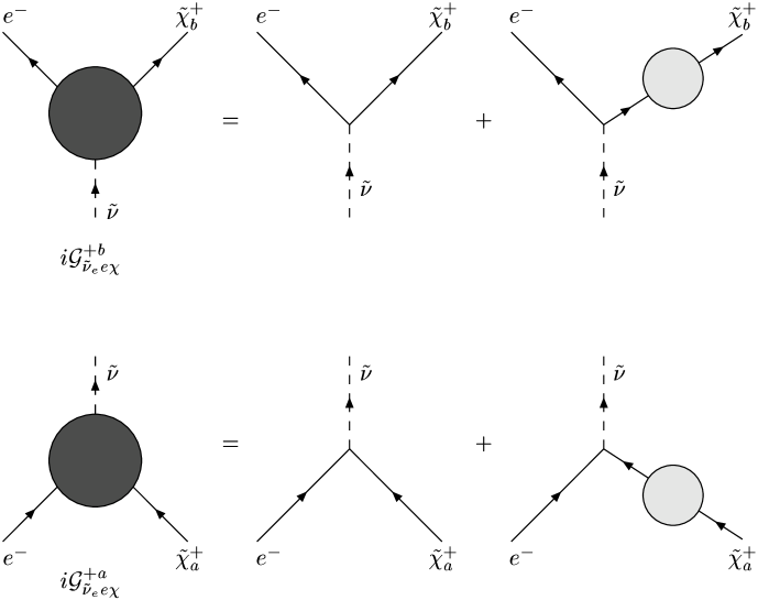
Figure 3: One–loop renormalized $e^{-}\tilde{\nu}_{e}\tilde{\chi}^{+}$ vertex functions.

Finally, we consider the $e^{+}\tilde{\nu}_{e}\tilde{\chi}^{+}_{b}$ and $e^{-}\tilde{\nu}_{e}\tilde{\chi}^{-}_{a}$ vertices, whose renormalization is represented in Fig. 3. If the one–loop graph is attached to the external $\tilde{\chi}^{+}_{b}$ chargino we find a contribution to the sneutrino form factor given by

$$F_{\tilde{\nu}_{e}}^{+}={{gV_{i1}}\over{m_{\chi_{b}}^{2}-m_{\chi_{i}}^{2}}}\Big{[}m_{\chi_{b}}\widetilde{A}_{ib}^{-}+m_{\chi_{i}}\widetilde{A}_{ib}^{+}+m_{\chi_{b}}(m_{\chi_{b}}\widetilde{B}_{ib}^{+}+m_{\chi_{i}}\widetilde{B}_{ib}^{-})\Big{]}$$ (4.11)

with $i\neq b$ and the all the functions $\widetilde{A}^{\pm}(k_{2}^{2})$ and $\widetilde{B}^{\pm}(k_{2}^{2})$ are evaluated at $k_{2}^{2}=m_{\chi_{b}}^{2}$. If the one–loop graph is attached to the external $\tilde{\chi}^{-}_{a}$ chargino we get

$$F_{\tilde{\nu}_{e}}^{-}=-{{gV_{i1}^{*}}\over{m_{\chi_{a}}^{2}-m_{\chi_{i}}^{2}}}\Big{[}m_{\chi_{a}}\widetilde{A}_{ai}^{+}+m_{\chi_{i}}\widetilde{A}_{ai}^{-}+m_{\chi_{a}}(m_{\chi_{a}}\widetilde{B}_{ai}^{+}+m_{\chi_{i}}\widetilde{B}_{ai}^{-})\Big{]}$$ (4.12)

with $i\neq a$ and the all the functions $\widetilde{A}^{\pm}(k_{1}^{2})$ and $\widetilde{B}^{\pm}(k_{1}^{2})$ are evaluated at $k_{1}^{2}=m_{\chi_{a}}^{2}$.

4.3 Chargino Masses and Wavefunction Renormalization

The unrenormalized chargino two–point functions in eq. (4.6) can be decomposed into two terms:

$$\Sigma_{\chi\chi}^{ij}(p)=\Sigma_{\chi\chi,1}^{ij}(p)+\gamma_{5}\Sigma_{\chi\chi,5}^{ij}(p)\,.$$ (4.13)

The inverse propagator at one–loop is then obtained by adding this self energy, previously renormalized according to the $\overline{MS}$ scheme, to the tree level propagator with the tree level mass promoted to a running mass

$$\Gamma^{(2)}_{\chi\chi}(p)=p_{\mu}\gamma^{\mu}-m_{\chi_{i}}(Q)+\widetilde{\Sigma}_{\chi\chi}^{ii}(p,Q)$$ (4.14)

The full propagator is essentially just the inverse of $\Gamma^{(2)}_{\chi\chi}$, so the physical pole mass is given by the zero of this function, in the limit where $p_{\mu}\gamma^{\mu}\longrightarrow m_{\chi_{i}}$, and may be found with the aid of the following equation:

$$\widetilde{Z}_{\chi_{i}}^{-1}\,\overline{u}(p)\Big{[}p_{\mu}\gamma^{\mu}-m_{\chi_{i}}\Big{]}u(p)=\overline{u}(p)\Big{[}p_{\mu}\gamma^{\mu}-m_{\chi_{i}}(Q)+\widetilde{\Sigma}_{\chi\chi}^{ii}(p,Q)\Big{]}u(p)$$ (4.15)

where $u$ and $\overline{u}$ are two (on-shell) spinors, $m_{\chi_{i}}$ is the pole mass of the chargino $\tilde{\chi}_{i}$, $m_{\chi_{i}}(Q)$ is its running mass, and $\widetilde{\Sigma}_{\chi\chi}^{ij}(p,Q)$ is the renormalized chargino two–point function in the $\overline{MS}$ scheme. The quantity $\widetilde{Z}_{\chi_{i}}$ is the residual finite wavefunction renormalization in the $\overline{MS}$ scheme, which account for the fact that the residue of the $\overline{MS}$ propagator at the pole is not one, as we shall see later. $\widetilde{Z}_{\chi_{i}}$ corresponds to the finite ratio of the infinite wavefunction renormalization constants in the $\overline{MS}$ scheme and the on-shell scheme. When renormalization is performed in the $\overline{MS}$ scheme, each external $\tilde{\chi}_{i}$ line has a factor of $(\widetilde{Z}_{\chi_{i}})^{-1/2}$ associated with it, according to the LSZ reduction formula. The renormalized two–point function $\widetilde{\Sigma}_{\chi\chi}^{ij}(p,Q)$ is calculated simply by substracting the pole terms proportional to the regulator of dimensional regularization $\Delta$ defined in eq. (2.12). Since $\overline{u}(p)\gamma_{5}u(p)=0$, only $\widetilde{\Sigma}_{\chi\chi,1}^{ij}(p)$ survives. From here we deduce the relation between the pole and running chargino masses:

$$\Delta m_{\chi_{i}}\equiv m_{\chi_{i}}(Q)-m_{\chi_{i}}=\widetilde{A}_{ii}^{+}(m_{\chi_{i}}^{2})+\widetilde{A}_{ii}^{-}(m_{\chi_{i}}^{2})+m_{\chi_{i}}\Big{[}\widetilde{B}_{ii}^{+}(m_{\chi_{i}}^{2})+\widetilde{B}_{ii}^{-}(m_{\chi_{i}}^{2})\Big{]}$$ (4.16)

Note that since $Q$ is the subtraction point, the renormalized quantities $\widetilde{A}^{\pm}$ and $\widetilde{B}^{\pm}$ are explicitly functions of $Q$. We give all our results in terms of the physical mass, i.e., the pole mass $m_{\chi_{i}}$.

In order to determine $\widetilde{Z}_{\chi_{i}}$ we first find the one–particle reducible graph formed by the sum of an infinite number of one–particle irreducible two point functions $i\widetilde{\Sigma}_{\chi\chi}^{ii}(p,Q)$ connected in series:

$$\overline{u}(p){i\over{p_{\mu}\gamma^{\mu}-m_{\chi_{i}}(Q)}}\Bigg{\{}1+i\widetilde{\Sigma}_{\chi\chi}^{ii}(p,Q){i\over{p_{\mu}\gamma^{\mu}-m_{\chi_{i}}(Q)}}+...\Bigg{\}}u(p)=$$

$$\overline{u}(p){i\over{p_{\mu}\gamma^{\mu}-m_{\chi_{i}}(Q)+\widetilde{\Sigma}_{\chi\chi}^{ii}(p,Q)}}u(p)=\overline{u}(p){{i\widetilde{Z}_{\chi_{i}}}\over{p_{\mu}\gamma^{\mu}-m_{\chi_{i}}}}u(p)$$ (4.17)

and the last equality in eq. (4.17) tell us that after taking the limit $p^{2}\rightarrow m_{\chi_{i}}^{2}$ and $p_{\mu}\gamma^{\mu}u\rightarrow m_{\chi_{i}}u$, the effect of the radiative corrections is to introduce a finite renormalization factor given by

$$\widetilde{Z}_{\chi_{i}}=1-2m_{\chi_{i}}\bigg{[}\widetilde{A}^{\prime+}_{ii}+\widetilde{A}^{\prime-}_{ii}+m_{\chi_{i}}\Big{(}\widetilde{B}^{\prime+}_{ii}+\widetilde{B}^{\prime-}_{ii}\Big{)}\bigg{]}-\widetilde{B}^{+}_{ii}-\widetilde{B}^{-}_{ii}$$ (4.18)

where the prime indicate derivative with respect to the argument $p^{2}$, and all the functions are evaluated at $p^{2}=m_{\chi_{i}}^{2}$. Note that the terms proportional to $\gamma_{5}\Sigma_{\chi\chi,5}^{ij}(p)$ do not contribute either to the difference between the pole mass and the running mass, or to the wavefunction renormalisation factor in eq.(4.18), since $\bar{u}(p)\gamma_{5}u(p)=0$.

Now we turn to the wave function renormalizations relevant to the process under consideration. We start with the vertices $Z\tilde{\chi}^{+}\tilde{\chi}^{-}$, as shown in Fig. 2. If the one–loop graph is attached to $\tilde{\chi}^{+}_{b}$ (Fig. 2d), we need to calculate the following amplitude:

$$\overline{u}(k_{2})[{\cal G}_{Z\chi\chi}^{ab}]^{2d}\,v(k_{1}) = -i{g\over{2c_{W}}}\overline{u}(k_{2})\Big{[}\widetilde{\Sigma}_{\chi\chi,1}^{bb}(k_{2})+\gamma_{5}\widetilde{\Sigma}_{\chi\chi,5}^{bb}(k_{2})-\Delta m_{\chi_{b}}\Big{]}$$

$$\times{1\over{k_{2}^{\nu}\gamma_{\nu}-m_{\chi_{b}}}}\gamma^{\mu}\Big{[}O^{\prime L}_{ab}(1-\gamma_{5})+O^{\prime R}_{ab}(1+\gamma_{5})\Big{]}v(k_{1})$$

The term proportional to $\widetilde{\Sigma}_{\chi\chi,5}^{bb}(k_{2})$ is simply evaluated by taking the spinors on shell and using $\overline{u}(k_{2})\gamma_{5}(k_{2}^{\nu}\gamma_{\nu}-m_{\chi_{b}})^{-1}=\overline{u}(k_{2})\gamma_{5}(-2m_{\chi_{b}})^{-1}$. For the term proportional to $\widetilde{\Sigma}_{\chi\chi,1}^{bb}(k_{2})$, more care is needed because of the pole from the propagator acting on an on-shell spinor. The mass difference $\Delta m_{\chi_{b}}$ appears because in the tree level amplitude a tree level external chargino propagator is truncated by an on–shell inverse propagator

$${1\over{k_{2}^{\nu}\gamma_{\nu}-m_{\chi_{b}}(Q)}}(k_{2}^{\nu}\gamma_{\nu}-m_{\chi_{b}})=1+{{\Delta m_{\chi_{b}}}\over{k_{2}^{\nu}\gamma_{\nu}-m_{\chi_{b}}}}+{\cal O}(2)$$ (4.20)

introducing precisely the $\Delta m_{\chi_{b}}$ in eq. (4.3) and neglecting terms of two-loop order. Of course, $\Delta m_{\chi_{b}}$ vanishes if we work in an on–shell scheme instead. Using eq. (4.16) we see that this term gives rise to a factor of $\widetilde{Z}_{\chi_{b}}-1$, with $Z_{\chi_{i}}$ given in eq. (4.18). Combining this with the factor of $(\widetilde{Z}_{\chi_{b}})^{-1/2}$ for the external $\tilde{\chi}_{b}$ line we obtain the following contributions to the $F_{Z0}^{\pm}$ form factors:

$$F_{Z0}^{+} = -{g\over{2c_{W}}}O^{\prime L}_{ab}\bigg{[}{1\over{2m_{\chi_{b}}}}(\widetilde{A}_{bb}^{-}-\widetilde{A}_{bb}^{+})-\widetilde{B}_{bb}^{-}-m_{\chi_{b}}(\widetilde{A}^{\prime+}_{bb}+\widetilde{A}^{\prime-}_{bb})-m_{\chi_{b}}^{2}(\widetilde{B}^{\prime+}_{bb}+\widetilde{B}^{\prime-}_{bb})\bigg{]}$$

$$F_{Z0}^{-} = -{g\over{2c_{W}}}O^{\prime R}_{ab}\bigg{[}{1\over{2m_{\chi_{b}}}}(\widetilde{A}_{bb}^{+}-\widetilde{A}_{bb}^{-})-\widetilde{B}_{bb}^{+}-m_{\chi_{b}}(\widetilde{A}^{\prime+}_{bb}+\widetilde{A}^{\prime-}_{bb})-m_{\chi_{b}}^{2}(\widetilde{B}^{\prime+}_{bb}+\widetilde{B}^{\prime-}_{bb})\bigg{]}$$

where the prime represent the derivative with respect to $p^{2}$ and all the functions are evaluated at $p^{2}=m_{\chi_{b}}^{2}$. In a similar way, if the one–loop graph is attached to $\tilde{\chi}^{+}_{a}$ (Fig. 2e), the amplitude to be calculated is

$$\overline{u}(k_{2})[{\cal G}_{Z\chi\chi}^{ab}]^{2e}\,v(k_{1}) = i{g\over{2c_{W}}}\overline{u}(k_{2})\gamma^{\mu}\Big{[}O^{\prime L}_{ba}(1-\gamma_{5})+O^{\prime R}_{ba}(1+\gamma_{5})\Big{]}{1\over{k_{1}^{\nu}\gamma_{\nu}+m_{\chi_{a}}}}$$ (4.22)

$$\times\Big{[}\widetilde{\Sigma}_{\chi\chi,1}^{aa}(-k_{1})+\gamma_{5}\widetilde{\Sigma}_{\chi\chi,5}^{aa}(-k_{1})-\Delta m_{\chi_{a}}\Big{]}v(k_{1})$$

Following similar steps to those for the self-energy insertion on the $\tilde{\chi}_{b}^{+}$ line we find that these contributions to the $F_{Z0}^{\pm}$ form factors are

$$F_{Z0}^{+} = -{g\over{2c_{W}}}O^{\prime L}_{ba}\bigg{[}{1\over{2m_{\chi_{a}}}}(\widetilde{A}_{aa}^{+}-\widetilde{A}_{aa}^{-})-\widetilde{B}_{aa}^{-}-m_{\chi_{a}}(\widetilde{A}^{\prime+}_{aa}+\widetilde{A}^{\prime-}_{aa})-m_{\chi_{a}}^{2}(\widetilde{B}^{\prime+}_{aa}+\widetilde{B}^{\prime-}_{aa})\bigg{]}$$

$$F_{Z0}^{-} = -{g\over{2c_{W}}}O^{\prime R}_{ba}\bigg{[}{1\over{2m_{\chi_{a}}}}(\widetilde{A}_{aa}^{-}-\widetilde{A}_{aa}^{+})-\widetilde{B}_{aa}^{+}-m_{\chi_{a}}(\widetilde{A}^{\prime+}_{aa}+\widetilde{A}^{\prime-}_{aa})-m_{\chi_{a}}^{2}(\widetilde{B}^{\prime+}_{aa}+\widetilde{B}^{\prime-}_{aa})\bigg{]}$$

and every function is evaluated at $m_{\chi_{a}}^{2}$.

We now turn to the vertices $\gamma\chi^{+}\chi^{-}$. The procedure is analogous and we just give the final results. If the one–loop graph is attached to the $\tilde{\chi}^{+}_{b}$ the we get the following contributions to the $F_{\gamma 0}$ form factors

$$F_{\gamma 0}^{+} = {e\over 2}\bigg{[}{1\over{2m_{\chi_{b}}}}(\widetilde{A}_{bb}^{-}-\widetilde{A}_{bb}^{+})-\widetilde{B}_{bb}^{-}-m_{\chi_{b}}(\widetilde{A}^{\prime+}_{bb}+\widetilde{A}^{\prime-}_{bb})-m_{\chi_{b}}^{2}(\widetilde{B}^{\prime+}_{bb}+\widetilde{B}^{\prime-}_{bb})\bigg{]}\delta_{ab}$$

$$F_{\gamma 0}^{-} = {e\over 2}\bigg{[}{1\over{2m_{\chi_{b}}}}(\widetilde{A}_{bb}^{+}-\widetilde{A}_{bb}^{-})-\widetilde{B}_{bb}^{+}-m_{\chi_{b}}(\widetilde{A}^{\prime+}_{bb}+\widetilde{A}^{\prime-}_{bb})-m_{\chi_{b}}^{2}(\widetilde{B}^{\prime+}_{bb}+\widetilde{B}^{\prime-}_{bb})\bigg{]}\delta_{ab}$$

where every function is evaluated at $m_{\chi_{b}}^{2}$. Now, if the one–loop graph is attached to $\tilde{\chi}^{+}_{a}$ we get

$$F_{\gamma 0}^{+} = {e\over 2}\bigg{[}{1\over{2m_{\chi_{a}}}}(\widetilde{A}_{aa}^{-}-\widetilde{A}_{aa}^{+})-\widetilde{B}_{aa}^{+}-m_{\chi_{a}}(\widetilde{A}^{\prime+}_{aa}+\widetilde{A}^{\prime-}_{aa})-m_{\chi_{a}}^{2}(\widetilde{B}^{\prime+}_{aa}+\widetilde{B}^{\prime-}_{aa})\bigg{]}\delta_{ab}$$

$$F_{\gamma 0}^{-} = {e\over 2}\bigg{[}{1\over{2m_{\chi_{a}}}}(\widetilde{A}_{aa}^{+}-\widetilde{A}_{aa}^{-})-\widetilde{B}_{aa}^{-}-m_{\chi_{a}}(\widetilde{A}^{\prime+}_{aa}+\widetilde{A}^{\prime-}_{aa})-m_{\chi_{a}}^{2}(\widetilde{B}^{\prime+}_{aa}+\widetilde{B}^{\prime-}_{aa})\bigg{]}\delta_{ab}$$

where every function is evaluated at $m_{\chi_{a}}^{2}$.

In the case of $e^{\pm}\tilde{\nu}_{e}\tilde{\chi}^{\mp}_{b}$ vertices, the procedure is analogous, with the only extra complication given by the handling of the charge conjugation matrix $C$ in the Feynman rules. If the one–loop graph is attached to the $\tilde{\chi}^{+}_{b}$ the we get the following contribution to $F_{\tilde{\nu}_{e}}^{+}$

$$F_{\tilde{\nu}_{e}}^{+}={g\over 2}V_{b1}\bigg{[}{1\over{2m_{\chi_{b}}}}(\widetilde{A}_{bb}^{-}-\widetilde{A}_{bb}^{+})-\widetilde{B}_{bb}^{-}-m_{\chi_{b}}(\widetilde{A}^{\prime+}_{bb}+\widetilde{A}^{\prime-}_{bb})-m_{\chi_{b}}^{2}(\widetilde{B}^{\prime+}_{bb}+\widetilde{B}^{\prime-}_{bb})\bigg{]}$$ (4.26)

with every function is evaluated at $m_{\chi_{b}}^{2}$. And finally, if the one–loop graph is attached to $\tilde{\chi}^{+}_{a}$ we get a contribution to $F_{\tilde{\nu}_{e}}^{-}$ given by

$$F_{\tilde{\nu}_{e}}^{-}=-{g\over 2}V_{a1}^{*}\bigg{[}{1\over{2m_{\chi_{a}}}}(\widetilde{A}_{aa}^{+}-\widetilde{A}_{aa}^{-})-\widetilde{B}_{aa}^{+}-m_{\chi_{a}}(\widetilde{A}^{\prime+}_{aa}+\widetilde{A}^{\prime-}_{aa})-m_{\chi_{a}}^{2}(\widetilde{B}^{\prime+}_{aa}+\widetilde{B}^{\prime-}_{aa})\bigg{]}$$ (4.27)

with every function is evaluated at $m_{\chi_{a}}^{2}$.

5 Results

In this section we calculate numerically the radiatively corrected chargino production cross section and compare it with the tree level. We start with a center of mass energy of $\sqrt{s}=192$ GeV relevant for LEP2, and consider the case $\mu<0$, where $\mu$ is the supersymmetric Higgs mass parameter in the superpotential. Figs. 4 to 7 correspond to this center of mass energy. Radiative corrections to this cross section are parametrized by the squark soft masses which we take degenerate $M_{Q}=M_{U}=M_{D}$, and by the trilinear soft mass parameters $A\equiv A_{U}=A_{D}$, also taken degenerate. This choice is done at the weak scale and it is made for simplicity, i.e., should not be confused with universality of minimal supergravity at the unification scale.

Figure 4: One–loop and tree level chargino production cross section as a function of $\tan\beta$, for 192 GeV center of mass energy.

In Fig. 4 we plot $\sigma(e^{+}e^{-}\rightarrow\tilde{\chi}^{+}_{1}\tilde{\chi}^{-}_{1})$ as a function of $\tan\beta$, for a constant value of the chargino mass $m_{\chi^{\pm}_{1}}=90$ GeV, the sneutrino mass $m_{\tilde{\nu}_{e}}=100$ GeV, and the gaugino mass $M=200$ GeV. The tree level cross section is in the solid line and decreases from 1.9 pb. to 0.9 pb. when $\tan\beta$ increases from 0.5 to 100. Three radiatively corrected curves are presented, and they are parametrized by $M_{Q}=A=200$ GeV (dots), $M_{Q}=A=600$ GeV (dashes), and $M_{Q}=A=1$ TeV (dotdashes). We observe that radiative corrections are positive and grow with the squark mass parameters. The maximum value of the corrections vary from $5\%$ at high $\tan\beta$ to $22\%$ at small $\tan\beta$. A logarithmic growth of quantum corrections with the squark mass parameters is observed, as it should be. Nevertheless, this logarithmic dependence is lost if $\tan\beta<1$ or $\tan\beta\stackrel{{\scriptstyle>}}{{{}_{\sim}}}30$, as can be seen from the figure. The reason is that at those values of $\tan\beta$ there is no longer a single scale of squark masses, specially for $M_{Q}=A=200$ GeV where the squark masses range from 100 GeV to 370 GeV. It is worth pointing out that the value of $\mu$ is not constant along the curves because it is fixed by the constant value of the chargino mass $m_{\tilde{\chi}^{\pm}_{1}}$.

Figure 5: One–loop and tree level chargino production cross section as a function of the chargino mass $m_{\chi^{\pm}_{1}}$, for 192 GeV center of mass energy.

In Fig. 5 we explore the dependence of the radiatively corrected cross section $\sigma(e^{+}e^{-}\rightarrow\tilde{\chi}^{+}_{1}\tilde{\chi}^{-}_{1})$ on the chargino mass $m_{\chi^{\pm}_{1}}$ for $\sqrt{s}=192$ GeV. We keep constant the sneutrino mass $m_{\tilde{\nu}_{e}}=100$ GeV, the gaugino mass $M=200$ GeV, and $\tan\beta=10$. The tree level cross section decreases from 1.8 pb. for $m_{\chi^{\pm}_{1}}=75$ GeV to 0.33 pb. for $m_{\chi^{\pm}_{1}}=95$ GeV and continues to zero at the kinematic limit. Quantum corrections, on the other hand, grow with the chargino mass from $11\%$ for $m_{\chi^{\pm}_{1}}=75$ GeV to $16\%$ for $m_{\chi^{\pm}_{1}}=95$ GeV when $M_{Q}=A=1$ TeV. The chargino mass $m_{\chi^{\pm}_{1}}$ in this section corresponds to the pole mass given in eq. (4.16). In Fig. 5, the running chargino mass is $1\%$ smaller than the pole mass for $M_{Q}=A=1$ TeV and the correction decreases with smaller squark mass parameters.

Figure 6: One–loop and tree level chargino production cross section as a function of the sneutrino mass $m_{\tilde{\nu}_{e}}$, for 192 GeV center of mass energy.

The dependence of the cross section $\sigma(e^{+}e^{-}\rightarrow\tilde{\chi}^{+}_{1}\tilde{\chi}^{-}_{1})$ on the electron–type sneutrino mass is shown in Fig. 6, where we take the chargino mass $m_{\chi^{\pm}_{1}}=90$ GeV, the gaugino mass $M=200$ GeV, and $\tan\beta=10$. Charginos can be produced in the t–channel with an intermediate $\tilde{\nu}_{e}$, and in the s–channel with intermediate $Z$ and $\gamma$. The interference between the t–channel and the s–channel is negative, and this is the reason why the cross section decreases when the sneutrino becomes lighter. The tree level cross section varies from 0.45 pb. when $m_{\tilde{\nu}_{e}}=45$ GeV to 1.9 pb when $m_{\tilde{\nu}_{e}}=500$ GeV. On the other hand, radiative corrections are larger when the sneutrino is lighter, going from $28\%$ for $m_{\tilde{\nu}_{e}}=45$ GeV to $3.5\%$ for $m_{\tilde{\nu}_{e}}=500$ GeV if $M_{Q}=A=1$ TeV. Smaller corrections are found if the squark mass parameters are decreased.

The last graph with center of mass energy $\sqrt{s}=192$ GeV is Fig. 7, where we plot the chargino production cross section $\sigma(e^{+}e^{-}\rightarrow\tilde{\chi}^{+}_{1}\tilde{\chi}^{-}_{1})$ as a function of the $SU(2)$ gaugino mass $M$, while keeping constant the chargino mass $m_{\chi^{\pm}_{1}}=90$ GeV, the sneutrino mass $m_{\tilde{\nu}_{e}}=100$ GeV, and $\tan\beta=10$.

Figure 7: One–loop and tree level chargino production cross section as a function of the $SU(2)$ gaugino mass $M$, for 192 GeV center of mass energy.

The tree level cross section decreases from 1.6 pb. when $M=500$ GeV to a minimum of 0.22 pb. at around $M=105$ GeV, and grows again up to 0.34 pb. at $M=90$ GeV. Below this value of the gaugino mass $M$ there is no solution for $\mu<0$ which gives $m_{\chi^{\pm}_{1}}=90$ GeV. As before, the largest quantum corrections are found with $M_{Q}=A=1$ TeV. For $M$ close to 90 GeV the corrections are only of a few percent, but they grow fast until a maximum of $21\%$ at $M=140$ GeV. For larger values of the gaugino mass, the corrections slowly decrease until they reach the value $6\%$ at $M=500$ GeV.

In summary we can say that for a center of mass energy $\sqrt{s}=192$ GeV, relevant for LEP2, the radiative corrections to the production cross section of a pair of light charginos grow logarithmically with the squark mass parameters. The corrections are positive and typically $10\%$ to $15\%$ for $M_{Q}=A=1$ TeV, $8\%$ to $11\%$ for $M_{Q}=A=600$ GeV, and $3\%$ to $5\%$ for $M_{Q}=A=200$ GeV, with a maximum value of the order of $30\%$, $20\%$, and $10\%$ respectively, for the region of parameter space explored here.

Figure 8: One–loop and tree level chargino production cross section as a function of $\tan\beta$, for 500 GeV center of mass energy.

Now we turn to a center of mass energy given by $\sqrt{s}=500$ GeV, relevant for future $e^{+}e^{-}$ colliders. Fig. 8 to 11 correspond to this energy, where we continue working with $\mu<0$.

In Fig. 8 we plot the total cross section $\sigma(e^{+}e^{-}\rightarrow\tilde{\chi}^{+}_{1}\tilde{\chi}^{-}_{1})$ as a function of $\tan\beta$ for a fixed value of the chargino mass $m_{\chi^{\pm}_{1}}=120$ GeV, the sneutrino mass $m_{\tilde{\nu}_{e}}=150$ GeV, and the gaugino mass $M=200$ GeV. The behaviour of the tree–level cross section is similar to the same curve with the previous center of mass energy, decreasing from 0.5 pb. at low $\tan\beta$ to 0.24 pb. at large $\tan\beta$. The corrections are positive and grow logarithmically with the squark mass parameters in the central region of $\tan\beta$, but this is not so in the extremes for the reason explained before. Furthermore, the curve corresponding to $M_{Q}=A=200$ GeV has to be truncated because if $\tan\beta\stackrel{{\scriptstyle<}}{{{}_{\sim}}}0.7$ we have $m_{\tilde{t}_{1}}\stackrel{{\scriptstyle<}}{{{}_{\sim}}}100$ GeV, and if $\tan\beta\stackrel{{\scriptstyle>}}{{{}_{\sim}}}70$ we get $m_{\tilde{b}_{1}}\stackrel{{\scriptstyle<}}{{{}_{\sim}}}100$ GeV. The maximum value of the corrections occurs at a point slightly over $\tan\beta=1$ and corresponds to $13\%$, $10\%$, and $5\%$ for squark mass parameters equal to 1000, 600, and 200 GeV respectively.

Figure 9: One–loop and tree level chargino production cross section as a function of of the chargino mass $m_{\chi^{\pm}_{1}}$, for 500 GeV center of mass energy.

The dependence of the total cross section $\sigma(e^{+}e^{-}\rightarrow\tilde{\chi}^{+}_{1}\tilde{\chi}^{-}_{1})$ as a function of the chargino mass is shown in Fig. 9. We consider the case $m_{\tilde{\nu}_{e}}=150$ GeV, $M=200$ GeV, and $\tan\beta=40$. The values of the chargino mass shown are the physical pole mass, which is at most $1.6\%$ larger than the running mass. Values of $m_{\tilde{\chi}_{1}^{\pm}}$ larger than 200 GeV are not displayed because there is no solution for $\mu$ compatible with those values of the chargino mass. In fact, $|\mu|$ grows as we approach to $m_{\tilde{\chi}_{1}^{\pm}}=200$ GeV and diverges at that point. Furthermore, large values of $|\mu|$ and the large value of $\tan\beta$ chosen induce a large sbottom mixing, and as a consequence the curve corresponding to $M_{Q}=A=200$ GeV is truncated because for example we get $m_{\tilde{b}_{1}}\stackrel{{\scriptstyle<}}{{{}_{\sim}}}100$ if $m_{\tilde{\chi}_{1}^{\pm}}\stackrel{{\scriptstyle>}}{{{}_{\sim}}}174$ GeV. Radiative corrections for $M_{Q}=A=1$ TeV are positive for small chargino masses and reach a maximum value of $8\%$, and they are negative for large $m_{\tilde{\chi}_{1}^{\pm}}$ with a maximum value of $-4\%$.

In Fig. 10 we plot $\sigma(e^{+}e^{-}\rightarrow\tilde{\chi}^{+}_{1}\tilde{\chi}^{-}_{1})$ in terms of the sneutrino mass $m_{\tilde{\nu}_{e}}$, for a constant value of the chargino mass $m_{\tilde{\chi}_{1}^{\pm}}=120$ GeV, the gaugino mass parameter $M=200$ GeV, and $\tan\beta=40$.

Figure 10: One–loop and tree level chargino production cross section as a function of the sneutrino mass $m_{\tilde{\nu}_{e}}$, for 500 GeV center of mass energy.

Due to the negative interference between the s–channel and the t–channel chargino production, the total cross section has a minimum at a certain value of the sneutrino mass. This minimum is shifted by radiative corrections from $m_{\tilde{\nu}_{e}}\approx 100$ GeV at tree level to $m_{\tilde{\nu}_{e}}\approx 90$ GeV at one–loop. Quantum corrections are larger for $M_{Q}=A=1$ TeV and have a maximum value of $8\%$ for medium values of the sneutrino mass.

In the last graph corresponding to $\sqrt{s}=500$ GeV we have the production cross section $\sigma(e^{+}e^{-}\rightarrow\tilde{\chi}^{+}_{1}\tilde{\chi}^{-}_{1})$ as a function of the gaugino mass $M$, and it is plotted in Fig. 11. We consider $m_{\tilde{\chi}_{1}^{\pm}}=120$ GeV, $m_{\tilde{\nu}_{e}}=150$ GeV, and $\tan\beta=40$. The tree level cross section has a minimum at $M\approx 180$ GeV which is displaced to $M\approx 173$ GeV by radiative corrections. These corrections are positive most of the time, reaching a maximum of $9\%$ when $M_{Q}=A=1$ TeV, but can be slightly negative at small values of the gaugino mass. The value of $|\mu|$ grows as we approach $M=120$ GeV, and consequently the curve corresponding to $M_{Q}=A=200$ GeV is truncated because $m_{\tilde{t}_{1}}$ is too light.

Figure 11: One–loop and tree level chargino production cross section as a function of the $SU(2)$ gaugino mass $M$, for 500 GeV center of mass energy.

Now we summarize the results corresponding to a center of mass energy given by $\sqrt{s}=500$ GeV. As before, for the region of parameter space explored here, we observe a logarithmic growth of the radiative corrections with the squark mass parameters only for medium values of $\tan\beta$. For extreme values of $\tan\beta$ there is no longer a unique squark mass scale due to large mass splitings. Corrections are smaller than the ones found for the previous center of mass energy, reaching maximum values of $13\%$, $11\%$, and $5\%$ for squark mass parameters equal to 1000, 600, and 200 GeV respectively. Contrary to the previous case, we find here negative corrections, reaching extreme values of $-4\%$, $-2.5\%$, and $-0.2\%$ respectively.

The last value of the center of mass energy we analyze here corresponds to an electron–positron collider with $\sqrt{s}=2$ TeV. Relevant to this energy we have Figs. 12 to 15. Again, we study the production of a pair of light charginos with $\mu<0$, but this time we concentrate on a very heavy chargino with $m_{\tilde{\chi}_{1}^{\pm}}=700$ GeV.

Figure 12: One–loop and tree level chargino production cross section as a function of $\tan\beta$, for 2 TeV center of mass energy.

We plot in Fig. 12 the total cross section $\sigma(e^{+}e^{-}\rightarrow\tilde{\chi}^{+}_{1}\tilde{\chi}^{-}_{1})$ in terms of $\tan\beta$ for $\sqrt{s}=2$ TeV. We take $m_{\tilde{\chi}_{1}^{\pm}}=700$ GeV, $m_{\tilde{\nu}_{e}}=200$, and $M=1$ TeV. The lowest value of squark mass parameters we consider is $M_{Q}=A=300$ GeV (dotted line). This is done in order to have reasonable squark masses. In fact, acceptable squark masses are found only if $2\stackrel{{\scriptstyle<}}{{{}_{\sim}}}\tan\beta\stackrel{{\scriptstyle<}}{{{}_{\sim}}}35$ and the restrictions on $\tan\beta$ are stronger for smaller squark mass parameters. The peak observed in the curve $M_{Q}=A=600$ GeV at $\tan\beta\approx 40$ is physical and corresponds to the threshold $m_{\tilde{\chi}_{1}^{\pm}}=m_{t}+m_{\tilde{b}_{1}}$ where a chargino can decay on–shell to a top quark plus the lightest bottom squark $\tilde{b}_{1}$. The largest radiative corrections are found for $M_{Q}=A=600$ GeV and can have either sign. The extreme values are $32\%$ at low $\tan\beta$ and $-16\%$ at high $\tan\beta$.

In Fig. 13 we have $\sigma(e^{+}e^{-}\rightarrow\tilde{\chi}^{+}_{1}\tilde{\chi}^{-}_{1})$ as a function of the pole chargino mass $m_{\tilde{\chi}_{1}^{\pm}}$ for a constant value of the sneutrino mass $m_{\tilde{\nu}_{e}}=200$, the gaugino mass $M=1$ TeV, and $\tan\beta=0.8$. The pole chargino mass is at most $1.5\%$ smaller that the running mass. The curve corresponding to $M_{Q}=A=300$ GeV is truncated because for $m_{\tilde{\chi}_{1}^{\pm}}\stackrel{{\scriptstyle>}}{{{}_{\sim}}}260$ GeV we have $m_{\tilde{t}_{1}}\stackrel{{\scriptstyle<}}{{{}_{\sim}}}100$ GeV.

Figure 13: One–loop and tree level chargino production cross section as a function of of the chargino mass $m_{\chi^{\pm}_{1}}$, for 2 TeV center of mass energy.

The peak in the curve $M_{Q}=A=600$ GeV close to $m_{\tilde{\chi}_{1}^{\pm}}=780$ GeV is the same threshold found in the previous figure where $m_{\tilde{\chi}_{1}^{\pm}}=m_{t}+m_{\tilde{b}_{1}}$. Radiative corrections are larger for $M_{Q}=A=600$ GeV and can go up to $44\%$, but with typical values of the order of $10\%$. They can also be negative reaching values of $-12\%$ for $M_{Q}=A=1$ TeV.

The dependence of the total cross section $\sigma(e^{+}e^{-}\rightarrow\tilde{\chi}^{+}_{1}\tilde{\chi}^{-}_{1})$ on the sneutrino mass $m_{\tilde{\nu}_{e}}$ is shown in Fig. 14, where we keep constant the value of the chargino mass $m_{\tilde{\chi}_{1}^{\pm}}=700$ GeV, the $SU(2)$ gaugino mass $M=1$ TeV, and $\tan\beta=0.8$. We observe that the cross section depends very weakly on the sneutrino mass. The reason is that the sneutrino contribution is negligible because the lightest chargino is almost purely higgsino and therefore its coupling to an electron plus a sneutrino is very small. Since the $W$–boson mass is so small compared with $M$ and $\mu$, the sneutrino contribution would be sizable only if we take a gaugino mass close to the chargino mass. Quantum corrections in this case are positive, almost constant, and equal to $8\%$, $14\%$, and $3\%$ if the squark mass parameters are equal to 1000, 600, and 300 GeV respectively. The case $M_{Q}=A=600$ GeV is larger due to the proximity of the $m_{\tilde{\chi}_{1}^{\pm}}=m_{t}+m_{\tilde{b}_{1}}$ threshold (see Fig. 13).

Figure 14: One–loop and tree level chargino production cross section as a function of the sneutrino mass $m_{\tilde{\nu}_{e}}$, for 2 TeV center of mass energy.

The final plot with $\sqrt{s}=2$ TeV is Fig. 15, where we have the total cross section $\sigma(e^{+}e^{-}\rightarrow\tilde{\chi}^{+}_{1}\tilde{\chi}^{-}_{1})$ as a function of the gaugino mass $M$. The cross section is fairly constant for $M\stackrel{{\scriptstyle>}}{{{}_{\sim}}}750$ GeV and has a deep minimum centered at $M\approx 705$ GeV at tree level, which is shifted upwards in a few GeV by quantum corrections. In the region of constant cross section, radiative corrections are positive and larger for $M_{Q}=A=600$ GeV, and are of the order of $15\%$. In the region around the minimum, radiative corrections are even larger and can have either sign, with extreme values that can go up to $100\%$ and down to $-26\%$.

We summarize now our findings at $\sqrt{s}=2$ TeV. In this case, due to the fact that the chargino mass is heavy and can decay into on–shell squarks plus quarks, we find large radiative corrections close to the threshold. This makes the radiatively corrected cross section less regular than the previous cases, and with larger extreme values. We find that the maximum value for the correction can go up to $100\%$, and that can be negative also, with a extreme value of $-26\%$. Typically, we find corrections in the range between $-20\%$ to $20\%$.

Figure 15: One–loop and tree level chargino production cross section as a function of the $SU(2)$ gaugino mass $M$, for 2 TeV center of mass energy.

6 Conclusions

We have calculated the one–loop radiative corrections to the total production cross section of a pair of charginos in the MSSM. Using the diagramatic method we give formulas for the radiatively corrected $\sigma(e^{+}e^{-}\rightarrow\tilde{\chi}^{+}_{b}\tilde{\chi}^{-}_{a})$, where $\tilde{\chi}^{+}_{b}$ and $\tilde{\chi}^{-}_{a}$ are any of the two charginos. We work in the $\overline{MS}$ scheme and under the approximation where only top and bottom quarks and squarks are considered in the loops. We organize the calculation introducing form factors which renormalize the $Z\tilde{\chi}^{+}_{b}\tilde{\chi}^{-}_{a}$, $\gamma\tilde{\chi}^{+}_{b}\tilde{\chi}^{-}_{a}$, and $e^{\pm}\tilde{\nu}_{e}\tilde{\chi}^{\pm}_{a}$ vertices. Numerically, we concentrate on the production of a pair of light charginos in electron–positron colliders with center of mass energy given by 192, 500, and 2000 GeV and with $\mu<0$. Radiative corrections to $\sigma(e^{+}e^{-}\rightarrow\tilde{\chi}^{+}_{1}\tilde{\chi}^{-}_{1})$ are parametrized by the value of the squark mass parameters, which for simplicity we take equal at the weak scale $M_{Q}=M_{U}=M_{D}$ and $A\equiv A_{U}=A_{D}$. We explore the cross section varying the parameters which affect the chargino cross section at tree level: the ratio of vacuum expectation values $\tan\beta$, the $SU(2)$ gaugino mass $M$, the electron–type sneutrino mass $m_{\tilde{\nu}_{e}}$, and the lightest chargino mass $m_{\tilde{\chi}_{1}^{\pm}}$, which has been used instead of the supersymmetric mass parameter $\mu$ as an independent variable. For a center of mass energy $\sqrt{s}=192$ GeV we have found positive radiative corrections which are typically of $10\%$ to $15\%$ if $M_{Q}=A=1$ TeV and with a maximum value of $30\%$. For a center of mass energy of $\sqrt{s}=500$ GeV we find corrections with a maximum value of $13\%$ if $M_{Q}=A=1$ TeV, but also negative corrections are found, and with an extreme value of $-4\%$. If $\sqrt{s}=2$ TeV, radiative corrections are larger, and extreme values of $100\%$ and $-26\%$ can be found. No big differences are observed for the case $\mu>0$.

The calculation of the radiative corrections to the chargino pair production cross section reported here will enable us to interpret more reliably the chargino searches performed al LEP2 as lower limits on the chargino mass and, consequently, as exclusion zones in the parameter space. If charginos are discovered, this calculation will be essential in order to extract the value of the fundamental parameters of the theory from the experimental measurements.

Appendix A: Feynman Rules

In this Appendix we list the Feynman rules for the MSSM that we require in our calculations. These rules are adapted from Haber and Kane [13] and Gunion and Haber [14], although we have introduced a more compact notation for the vertices involving mass eigenstates as we shall explain.

Apart from the Standard Model Feynman rules, which we do not list here, there are three classes of vertex which are encountered in our calculations:

1. The $Z$ (and photon) - chargino - chargino vertices

2. The $Z$ (and photon) - squark - squark vertices

3. The quark- squark- chargino vertices

4. The lepton - slepton - chargino vertices

We begin by explaining the origin of chargino mass eigenstates. Suppose we write the components of the $\hat{W}$ superfield and the two Higgs superfields $\hat{H}_{U}$ and $\hat{H}_{D}$ as:

$$\hat{W}^{\pm}=(W_{\mu}^{\pm},\lambda^{\pm})$$

$$\hat{H}_{U}=\left(\begin{array}[]{c}(H_{U}^{0},\tilde{H}_{U}^{0})\\ (H_{U}^{-},\tilde{H}_{U}^{-})\end{array}\right)$$ (A.3)

$$\hat{H}_{D}=\left(\begin{array}[]{c}(H_{D}^{+},\tilde{H}_{D}^{+})\\ (H_{D}^{0},\tilde{H}_{D}^{0})\end{array}\right)$$ (A.6)

Then the chargino matrix is given by:

$$(\lambda^{-}\ \ \tilde{H}_{U}^{-})\left(\begin{array}[]{cc}M&\sqrt{2}m_{W}s_{\beta}\\ \sqrt{2}m_{W}c_{\beta}&\mu\end{array}\right)\left(\begin{array}[]{c}\lambda^{+}\\ \tilde{H}_{D}^{+}\end{array}\right)$$ (A.11)

In a standard notation $M$ is the soft supersymmetry breaking mass of the winos, $\mu$ is the supersymmetry preserving mass of the Higgsinos and the mixing between winos and Higgsinos originates from the supersymmetric version of the $W^{\pm}H^{\pm}H^{0}$ vertex in a two Higgs doublet model where the $W^{\pm}$ and $H^{\pm}$ are replaced by their superpartners and the $H^{0}$ is replaced by its vacuum expectation value.

Figure 16: $\gamma\chi^{+}\chi^{+}$ and $Z\chi^{+}\chi^{+}$ Feynman rules.

The chargino matrix is diagonalized by two independent unitary matrices $U$ and $V$:

$$U^{\ast}\left(\begin{array}[]{cc}M&\sqrt{2}m_{W}s_{\beta}\\ \sqrt{2}m_{W}c_{\beta}&\mu\end{array}\right)V^{-1}=\left(\begin{array}[]{cc}m_{\chi_{1}}&0\\ 0&m_{\chi_{2}}\end{array}\right)$$ (A.16)

where

$$2m_{\chi_{1,2}}=M^{2}+\mu^{2}+2m_{W}^{2}\\ \mp\sqrt{(M^{2}-\mu^{2})^{2}+4m_{W}^{4}c^{2}_{2\beta}+4m_{W}^{2}(M^{2}+\mu^{2}+2M\mu s_{2\beta})}$$ (A.17)

After diagonalization the four Weyl spinors $\lambda^{+},\lambda^{-},\tilde{H}_{D}^{+},\tilde{H}_{U}^{-}$ are related to four mass eigenstate Weyl spinors $\chi_{1}^{+},\chi_{2}^{+},\chi_{1}^{-},\chi_{2}^{-}$,

$$\left(\begin{array}[]{c}\chi_{1}^{+}\\ \chi_{2}^{+}\end{array}\right)=V\left(\begin{array}[]{c}\lambda^{+}\\ \tilde{H}_{D}^{+}\end{array}\right)$$ (A.22)

$$\left(\begin{array}[]{c}\chi_{1}^{-}\\ \chi_{2}^{-}\end{array}\right)=U\left(\begin{array}[]{c}\lambda^{-}\\ \tilde{H}_{U}^{-}\end{array}\right)$$ (A.27)

Clearly $\chi_{1}^{+}$ and $\chi_{1}^{-}$ have a common mass $m_{\chi_{1}}$. Similarly $\chi_{2}^{+}$ and $\chi_{2}^{-}$ have a common mass $m_{\chi_{2}}$. In view of this one may define Dirac spinors $\tilde{\chi}_{1}^{+}$ and $\tilde{\chi}_{2}^{+}$ as:

$$\tilde{\chi}_{1}^{+}=\left(\begin{array}[]{c}\chi_{1}^{+}\\ \bar{\chi}_{1}^{-}\end{array}\right)$$ (A.30)

$$\tilde{\chi}_{2}^{+}=\left(\begin{array}[]{c}\chi_{2}^{+}\\ \bar{\chi}_{2}^{-}\end{array}\right)$$ (A.33)

where $\bar{\chi}_{1}^{-}$ and $\bar{\chi}_{2}^{-}$ are the CP conjugates of the Weyl spinors ${\chi}_{1}^{-}$ and ${\chi}_{2}^{-}$.

When we write down the Feynman rules it will be in terms of these Dirac mass eigenstates $\tilde{\chi}_{1}^{+}$ and $\tilde{\chi}_{2}^{+}$ which are four-component spinors and have antiparticles $\tilde{\chi}_{1}^{-}$ and $\tilde{\chi}_{2}^{-}$.

In Fig. 16 the photon vertex is standard and the $Z$ vertex is in the notation of Haber and Kane where:

$$O^{{}^{\prime}L}_{ab} = -V_{a1}V^{\ast}_{b1}-\frac{1}{2}V_{a2}V^{\ast}_{b2}+\delta_{ab}s_{W}^{2}$$

$$O^{{}^{\prime}R}_{ab} = -U^{\ast}_{a1}U_{b1}-\frac{1}{2}U^{\ast}_{a2}U_{b2}+\delta_{ab}s_{W}^{2}$$ (A.34)

where $U$ and $V$ are the matrices which diagonalize the chargino mass matrix.

Figure 17: $\gamma\tilde{q}\tilde{q}$ and $Z\tilde{q}\tilde{q}$ Feynman rules.

We now turn to the squark vertices in Fig. 17. The photon coupling is standard, and the $Z$ coupling to the left and right handed stop and sbottom $\tilde{t}_{L},\tilde{t}_{R},\tilde{b}_{L},\tilde{b}_{R}$ are given in Haber and Kane as:

$$Z\tilde{t}_{L}\tilde{t}_{L} : \ \ \frac{ig}{2c_{W}}(-1+2e_{u}s_{W}^{2})(p+p^{\prime})^{\mu}$$

$$Z\tilde{t}_{R}\tilde{t}_{R} : \ \ \frac{ig}{2c_{W}}(e_{u}s_{W}^{2})(p+p^{\prime})^{\mu}$$

$$Z\tilde{b}_{L}\tilde{b}_{L} : \ \ \frac{ig}{2c_{W}}(1+2e_{d}s_{W}^{2})(p+p^{\prime})^{\mu}$$

$$Z\tilde{b}_{R}\tilde{b}_{R} : \ \ \frac{ig}{2c_{W}}(e_{d}s_{W}^{2})(p+p^{\prime})^{\mu}$$ (A.35)

where $e_{u}=2/3,e_{d}=-1/3$.

The coupling in Fig. 17 refers to the mass eigenstate squarks labelled by indices $i,j$, and involves a diagonalisation of the stop and sbottom mass matrices:

$$(\tilde{t}^{\ast}_{L},\tilde{t}^{\ast}_{R})\left(\begin{array}[]{cc}M_{Q}^{2}+m_{t}^{2}+\frac{1}{6}(4m_{W}^{2}-m_{Z}^{2})c_{2\beta}&m_{t}(A_{U}-\mu/t_{\beta})\\ m_{t}(A_{U}-\mu/t_{\beta})&M_{U}^{2}+m_{t}^{2}+\frac{2}{3}(m_{Z}^{2}-m_{W}^{2})c_{2\beta}\end{array}\right)\left(\begin{array}[]{c}\tilde{t}_{L}\\ \tilde{t}_{R}\end{array}\right)$$ (A.40)

(A.41)

$$(\tilde{b}^{\ast}_{L},\tilde{b}^{\ast}_{R})\left(\begin{array}[]{cc}M_{Q}^{2}+m_{b}^{2}-\frac{1}{6}(2m_{W}^{2}+m_{Z}^{2})c_{2\beta}&m_{b}(A_{D}-\mu t_{\beta})\\ m_{b}(A_{D}-\mu t_{\beta})&M_{D}^{2}+m_{b}^{2}-\frac{1}{3}(m_{Z}^{2}-m_{W}^{2})c_{2\beta}\end{array}\right)\left(\begin{array}[]{c}\tilde{b}_{L}\\ \tilde{b}_{R}\end{array}\right)$$ (A.46)

The mass eigenstates $\tilde{t}_{1},\tilde{t}_{2},\tilde{b}_{1},\tilde{b}_{2}$ are related to the original states $\tilde{t}_{L},\tilde{t}_{R},\tilde{b}_{L},\tilde{b}_{R}$ by rotations through angles $\alpha_{t}$ and $\alpha_{b}$:

$$\left(\begin{array}[]{c}\tilde{t}_{L}\\ \tilde{t}_{R}\end{array}\right)=R_{\alpha_{t}}^{\dagger}\left(\begin{array}[]{c}\tilde{t}_{1}\\ \tilde{t}_{2}\end{array}\right)$$ (A.51)

$$\left(\begin{array}[]{c}\tilde{b}_{L}\\ \tilde{b}_{R}\end{array}\right)=R_{\alpha_{b}}^{\dagger}\left(\begin{array}[]{c}\tilde{b}_{1}\\ \tilde{b}_{2}\end{array}\right)$$ (A.56)

where

$$R_{\alpha}=\left(\begin{array}[]{cc}c_{\alpha}&s_{\alpha}\\ -s_{\alpha}&c_{\alpha}\end{array}\right)$$ (A.59)

From the above results we obtain the couplings $\lambda^{ij}_{Z\tilde{t}\tilde{t}}$ and $\lambda^{ij}_{Z\tilde{b}\tilde{b}}$ used in Fig. 17:

$$\lambda^{ij}_{Z\tilde{t}\tilde{t}} = R_{\alpha_{t}}^{i1}R_{\alpha_{t}}^{j1}\frac{g}{2c_{W}}(-1+2e_{u}s_{W}^{2})+R_{\alpha_{t}}^{i2}R_{\alpha_{t}}^{j2}\frac{g}{2c_{W}}(e_{u}s_{W}^{2})$$

$$\lambda^{ij}_{Z\tilde{b}\tilde{b}} = R_{\alpha_{b}}^{i1}R_{\alpha_{b}}^{j1}\frac{g}{2c_{W}}(1+2e_{d}s_{W}^{2})+R_{\alpha_{b}}^{i2}R_{\alpha_{b}}^{j2}\frac{g}{2c_{W}}(e_{d}s_{W}^{2})$$ (A.60)

Figure 18: $q\tilde{q}\chi$ Feynman rules.

Next we consider the quark-squark-chargino vertices in Fig. 18. Again the index $i$ refers to squark mass eigenstates, and the index $a$ refers to chargino mass eigenstates. The Feynman rules for such vertices in the chargino mass eigenstate basis but involving left and right handed quarks were given in Gunion and Haber [14]. As pointed out by Gunion and Haber, and indicated in Fig. 18, one must be careful to distinguish between the two cases in which the arrow on the chargino line enters or leaves the vertex. In addition one will note the appearance of the charge conjugation matrix $C$ in the vertices involving the $b$ quark.

To understand these facts consider the standard model terms which appear in the interaction lagrangian between the $W^{\pm}$ and the top and bottom quarks:

$$gW^{+}_{\mu}\bar{t}_{L}\gamma^{\mu}b_{L}+gW^{-}_{\mu}\bar{b}_{L}\gamma^{\mu}t_{L}$$

These two terms may be represented by two diagrams, one involving the creation of a left handed top quark whose arrow leaves the vertex, and one involving the destruction of a left handed top quark whose arrow enters the vertex. Note that these two diagrams are not related by C or P but simply by Hermitian conjugation. Now the supersymmetric version of these standard model terms is:

$$\sqrt{2}g\bar{t}_{L}\lambda^{+}\tilde{b}_{L}+\sqrt{2}g\bar{b}_{L}\lambda^{-}\tilde{t}_{L}+\sqrt{2}g\bar{\lambda^{+}}t_{L}\tilde{b}_{L}^{\ast}+\sqrt{2}g\bar{\lambda^{-}}b_{L}\tilde{t}_{L}^{\ast}$$

Thus there are four independent supersymmetric vertices, corresponding to the $\lambda^{\pm}$ being created and destroyed at the vertex. We saw earlier that in terms of the Dirac spinors a four component mass eigenstate chargino $\tilde{\chi}_{a}^{+}$ contains both $\lambda^{+}$ and the CP conjugate of $\lambda^{-}$. In our convention that $\tilde{\chi}_{a}^{+}$ is the particle and $\tilde{\chi}_{a}^{-}$ is the antiparticle; we must take the CP conjugate of the terms involving $\lambda^{-}$, and this leads to the appearance of the $C$ matrix in the Feynman rules involving $\tilde{\chi}_{a}^{+}$, as given in Gunion and Haber.

Figure 19: $e^{\pm}\tilde{\nu}_{e}\chi^{\pm}$ Feynman rules.

By replacing the Gunion and Haber left and right handed quark fields by their mass eigenstates, and correcting the sign errors in the $\gamma_{5}$ matrices in Figs.22(b), 22(d), 23(b) and 23(d) of ref.[14] we find that the couplings that we have defined in Fig. 18 are given by:

$$\lambda_{\tilde{b}t\chi}^{+ia} = -\frac{g}{2}R^{i1}_{\alpha_{b}}U_{a1}+\frac{g}{2}\frac{m_{b}}{\sqrt{2}m_{W}c_{\beta}}R^{i2}_{\alpha_{b}}U_{a2}$$

$$\lambda_{\tilde{b}t\chi}^{-ia} = \frac{g}{2}\frac{m_{t}}{\sqrt{2}m_{W}s_{\beta}}R^{i1}_{\alpha_{b}}V_{a2}^{\ast}$$

$$\lambda_{\tilde{t}b\chi}^{+ia} = -\frac{g}{2}R^{i1}_{\alpha_{t}}V_{a1}+\frac{g}{2}\frac{m_{t}}{\sqrt{2}m_{W}s_{\beta}}R^{i2}_{\alpha_{t}}V_{a2}$$

$$\lambda_{\tilde{t}b\chi}^{-ia} = \frac{g}{2}\frac{m_{b}}{\sqrt{2}m_{W}c_{\beta}}R^{i1}_{\alpha_{t}}U_{a2}^{\ast}$$ (A.61)

Finally we note that the Feynman rules in Fig. 19 are obtained from Haber and Kane.

Appendix B: Passarino–Veltman Functions

In this appendix we list all the relevant PV functions, in terms of integrals over loop momenta performed in $n=4-2\epsilon$ dimensions.

B1: Tadpole integral

$$\int\frac{d^{n}k}{(2\pi)^{n}}\frac{1}{(k^{2}-m^{2})}=\frac{i}{16\pi^{2}}A_{0}(m^{2}).$$ (B.1)

B2: Two-point functions

$$\int\frac{d^{n}k}{(2\pi)^{n}}\frac{1}{(k^{2}-m_{1}^{2})((k+p)^{2}-m_{2})^{2}}=\frac{i}{16\pi^{2}}B_{0}(p^{2},m_{1}^{2},m_{2}^{2}).$$ (B.2)

$$\int\frac{d^{n}k}{(2\pi)^{n}}\frac{k^{\mu}}{(k^{2}-m_{1}^{2})((k+p)^{2}-m_{2})^{2}}=\frac{i}{16\pi^{2}}B_{1}(p^{2},m_{1}^{2},m_{2}^{2})\,p^{\mu}.$$ (B.3)

B3: Vertex functions

$$\int\frac{d^{n}k}{(2\pi)^{n}}\frac{1}{(k^{2}-m_{1}^{2})((k+p_{1})^{2}-m_{2})^{2}((k+p_{1}+p_{2})^{2}-m_{3}^{2})}=\frac{i}{16\pi^{2}}C_{0}$$ (B.4)

$$\int\frac{d^{n}k}{(2\pi)^{n}}\frac{k^{\mu}}{(k^{2}-m_{1}^{2})((k+p_{1})^{2}-m_{2})^{2}((k+p_{1}+p_{2})^{2}-m_{3}^{2})}=\frac{i}{16\pi^{2}}\left(C_{11}\,p_{1}^{\mu}+C_{12}\,p_{2}^{\mu}\right),$$ (B.5)

$$\int\frac{d^{n}k}{(2\pi)^{n}}\frac{k^{\mu}k^{\nu}}{(k^{2}-m_{1}^{2})((k+p_{1})^{2}-m_{2})^{2}((k+p_{1}+p_{2})^{2}-m_{3}^{2})}$$

$$=\frac{i}{16\pi^{2}}\left(C_{21}\,p_{1}^{\mu}p_{1}^{\nu}+C_{22}\,p_{2}^{\mu}p_{2}^{\nu}+C_{23}(p_{1}^{\mu}p_{2}^{\nu}+p_{2}^{\mu}p_{1}^{\nu})+C_{24}g^{\mu\nu}\right),$$ (B.6)

where the functions $C_{0},\,C_{ij}$ have arguments $(p_{1}^{2},p_{2}^{2},(p_{1}+p_{2})^{2},m_{1}^{2},m_{2}^{2},m_{3}^{2})$.

The exact form of the functions $A_{0},B_{i},C_{i},C_{ij}$ are given in [12]. The functions $A_{0},B_{0},B_{1},C_{24}$ are ultraviolet divergent and therefore contain the quantity $\Delta$ defined in eq. (2.12). After renormalisation, which corresponds to setting $\Delta=0$, the functions become finite and are denoted by a tilde, and depend on the subtraction point $Q$. For the purposes of our numerical calculations the subtraction point was taken to be $Q=m_{Z}$, so that the coupling constants used refer to running coupings at $m_{Z}$.

Appendix C: One-Loop 1PI Green’s Functions

In this Appendix we detail our results for the one-loop Feynman amplitudes obtained using the Feynman rules in Appendix A and expressed in terms of the PV functions in Appendix B. Although we shall present results for unrenormalised 1PI Greens functions, the contributions to the physical form factors are obtained from the renormalised 1PI Greens functions. The renormalised 1PI Greens functions are simply obtained by replacing the singular functions $A_{0},B_{0},B_{1},C_{24}$ by the corresponding tilded functions as explained at the end of the preceeding Appendix.

C1. Triangular Graphs

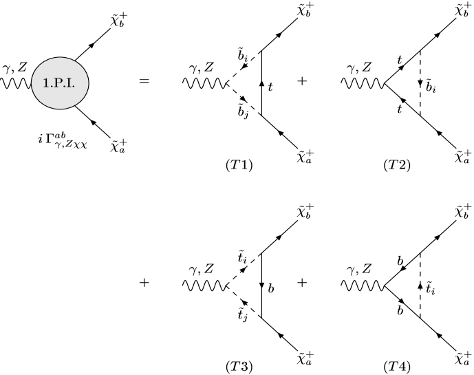
Figure 20: Unrenormalized one–particle irreducible triangular diagrams.

We begin with the one-loop triangular diagrams contributing to the Z-chargino-chargino vertex, and displayed in Fig. 20.

The Z vertex diagram $T1$ in Fig. 20 involving an internal top quark and two internal sbottom squarks is:

$$\!\!\!\!\!\!\!\!\!\![\Gamma_{Z\chi\chi}^{ab}]^{T1}\;\>=\;\>-{{N_{c}}\over{8\pi^{2}}}\sum_{i=1}^{2}\sum_{j=1}^{2}\lambda_{Z\tilde{b}\tilde{b}}^{ij}\Bigg{\{}\bigg{[}{\lambda_{\tilde{b}t\chi}^{+ib}}^{*}\lambda_{\tilde{b}t\chi}^{+ja}(1-\gamma_{5})+{\lambda_{\tilde{b}t\chi}^{-ib}}^{*}\lambda_{\tilde{b}t\chi}^{-ja}(1+\gamma_{5})\bigg{]}\Big{[}2C_{24}\gamma^{\mu}$$

$$\quad\qquad\qquad-m_{\chi_{a}}(2C_{21}+3C_{11}+C_{0})k_{1}^{\mu}-m_{\chi_{a}}(2C_{23}+C_{11}+2C_{12}+C_{0})k_{2}^{\mu}\Big{]}$$ (C.1)

$$+m_{\chi_{b}}\bigg{[}{\lambda_{\tilde{b}t\chi}^{+ib}}^{*}\lambda_{\tilde{b}t\chi}^{+ja}(1+\gamma_{5})+{\lambda_{\tilde{b}t\chi}^{-ib}}^{*}\lambda_{\tilde{b}t\chi}^{-ja}(1-\gamma_{5})\bigg{]}\Big{[}(2C_{23}+C_{12})k_{1}^{\mu}+(2C_{22}+C_{12})k_{2}^{\mu}\Big{]}$$

$$-m_{t}\bigg{[}{\lambda_{\tilde{b}t\chi}^{+ib}}^{*}\lambda_{\tilde{b}t\chi}^{-ja}(1-\gamma_{5})+{\lambda_{\tilde{b}t\chi}^{-ib}}^{*}\lambda_{\tilde{b}t\chi}^{+ja}(1+\gamma_{5})\bigg{]}\Big{[}(2C_{11}+C_{0})k_{1}^{\mu}+(2C_{12}+C_{0})k_{2}^{\mu}\Big{]}\Bigg{\}}$$

where the arguments of the PV functions $C_{0}$ and $C_{ij}$ are $(m_{\chi_{a}}^{2},m_{\chi_{b}}^{2},s;m_{\tilde{b}_{j}}^{2},m_{t}^{2},m_{\tilde{b}_{i}}^{2})$.

The Z vertex diagram $T2$ in Fig. 20 involving an internal sbottom squark and two internal top quarks is:

$$\!\!\!\!\!\!\!\!\!\![\Gamma_{Z\chi\chi}^{ab}]^{T2}\;\>=\;\>{{N_{c}g}\over{16\pi^{2}c_{W}}}\sum_{i=1}^{2}\Bigg{\{}$$

$$\bigg{[}(g_{V}^{t}+g_{A}^{t}){\lambda_{\tilde{b}t\chi}^{+ib}}^{*}\lambda_{\tilde{b}t\chi}^{+ia}(1-\gamma_{5})+(g_{V}^{t}-g_{A}^{t}){\lambda_{\tilde{b}t\chi}^{-ib}}^{*}\lambda_{\tilde{b}t\chi}^{-ia}(1+\gamma_{5})\bigg{]}\bigg{[}\Big{(}2C_{24}-B_{0}^{\chi_{b}\tilde{b}_{i}t}-(s$$

$$\quad-m_{\chi_{a}}^{2})C_{12}-m_{\chi_{a}}^{2}C_{11}-m_{t}^{2}C_{0}\Big{)}\gamma^{\mu}-2m_{\chi_{a}}(C_{21}+C_{11})k_{1}^{\mu}-2m_{\chi_{a}}(C_{23}+C_{12})k_{2}^{\mu}\bigg{]}$$

$$+m_{\chi_{b}}\bigg{[}(g_{V}^{t}+g_{A}^{t}){\lambda_{\tilde{b}t\chi}^{+ib}}^{*}\lambda_{\tilde{b}t\chi}^{+ia}(1+\gamma_{5})+(g_{V}^{t}-g_{A}^{t}){\lambda_{\tilde{b}t\chi}^{-ib}}^{*}\lambda_{\tilde{b}t\chi}^{-ia}(1-\gamma_{5})\bigg{]}\Big{[}m_{\chi_{a}}(C_{12}$$

$$\quad\qquad-C_{11})\gamma^{\mu}+2(C_{23}+C_{12})k_{1}^{\mu}+2(C_{22}+C_{12})k_{2}^{\mu}\Big{]}$$

$$-m_{t}\bigg{[}(g_{V}^{t}-g_{A}^{t}){\lambda_{\tilde{b}t\chi}^{+ib}}^{*}\lambda_{\tilde{b}t\chi}^{-ia}(1-\gamma_{5})+(g_{V}^{t}+g_{A}^{t}){\lambda_{\tilde{b}t\chi}^{-ib}}^{*}\lambda_{\tilde{b}t\chi}^{+ia}(1+\gamma_{5})\bigg{]}\Big{[}m_{\chi_{a}}C_{11}\gamma^{\mu}$$

$$\quad\qquad-2C_{12}k_{2}^{\mu}\Big{]}$$

$$-m_{t}m_{\chi_{b}}\bigg{[}(g_{V}^{t}-g_{A}^{t}){\lambda_{\tilde{b}t\chi}^{+ib}}^{*}\lambda_{\tilde{b}t\chi}^{-ia}(1+\gamma_{5})+(g_{V}^{t}+g_{A}^{t}){\lambda_{\tilde{b}t\chi}^{-ib}}^{*}\lambda_{\tilde{b}t\chi}^{+ia}(1-\gamma_{5})\bigg{]}C_{12}\gamma^{\mu}$$

$$+m_{t}\bigg{[}(g_{V}^{t}+g_{A}^{t}){\lambda_{\tilde{b}t\chi}^{+ib}}^{*}\lambda_{\tilde{b}t\chi}^{-ia}(1-\gamma_{5})+(g_{V}^{t}-g_{A}^{t}){\lambda_{\tilde{b}t\chi}^{-ib}}^{*}\lambda_{\tilde{b}t\chi}^{+ia}(1+\gamma_{5})\bigg{]}\Big{[}m_{\chi_{a}}(C_{11}+C_{0})\gamma^{\mu}$$

$$\quad\qquad+2(C_{11}+C_{0})k_{1}^{\mu}\Big{]}$$

$$+m_{t}m_{\chi_{b}}\bigg{[}(g_{V}^{t}+g_{A}^{t}){\lambda_{\tilde{b}t\chi}^{+ib}}^{*}\lambda_{\tilde{b}t\chi}^{-ia}(1+\gamma_{5})+(g_{V}^{t}-g_{A}^{t}){\lambda_{\tilde{b}t\chi}^{-ib}}^{*}\lambda_{\tilde{b}t\chi}^{+ia}(1-\gamma_{5})\bigg{]}(C_{12}+C_{0})\gamma^{\mu}$$

$$+m_{t}^{2}\bigg{[}(g_{V}^{t}-g_{A}^{t}){\lambda_{\tilde{b}t\chi}^{+ib}}^{*}\lambda_{\tilde{b}t\chi}^{+ia}(1-\gamma_{5})+(g_{V}^{t}+g_{A}^{t}){\lambda_{\tilde{b}t\chi}^{-ib}}^{*}\lambda_{\tilde{b}t\chi}^{-ia}(1+\gamma_{5})\bigg{]}C_{0}\gamma^{\mu}\Bigg{\}}$$ (C.2)

where the arguments of the PV functions $C_{0}$ and $C_{ij}$ are $(m_{\chi_{a}}^{2},m_{\chi_{b}}^{2},s;m_{t}^{2},m_{\tilde{b}_{i}}^{2},m_{t}^{2})$, and $B_{0}^{\tilde{\chi}_{b}\tilde{b}_{i}t}\equiv B_{0}(m_{\chi_{b}}^{2};m_{\tilde{b}_{i}}^{2},m_{t}^{2})$.

The Z vertex diagram $T3$ in Fig. 20 involving an internal bottom quark and two internal stop squarks is:

$$\!\!\!\!\!\!\!\!\!\![\Gamma_{Z\chi\chi}^{ab}]^{T3}\;\>=\;\>-{{N_{c}}\over{8\pi^{2}}}\sum_{i=1}^{2}\sum_{j=1}^{2}\lambda_{Z\tilde{t}\tilde{t}}^{ij}\Bigg{\{}\bigg{[}\lambda_{\tilde{t}b\chi}^{-ib}{\lambda_{\tilde{t}b\chi}^{-ja}}^{*}(1+\gamma_{5})+\lambda_{\tilde{t}b\chi}^{+ib}{\lambda_{\tilde{t}b\chi}^{+ja}}^{*}(1-\gamma_{5})\bigg{]}\Big{[}2C_{24}\gamma^{\mu}$$

$$\quad\qquad\qquad-m_{\chi_{a}}(2C_{21}+3C_{11}+C_{0})k_{1}^{\mu}-m_{\chi_{a}}(2C_{23}+C_{11}+2C_{12}+C_{0})k_{2}^{\mu}\Big{]}$$ (C.3)

$$+m_{\chi_{b}}\bigg{[}\lambda_{\tilde{t}b\chi}^{-ib}{\lambda_{\tilde{t}b\chi}^{-ja}}^{*}(1-\gamma_{5})+\lambda_{\tilde{t}b\chi}^{+ib}{\lambda_{\tilde{t}b\chi}^{+ja}}^{*}(1+\gamma_{5})\bigg{]}\Big{[}(2C_{23}+C_{12})k_{1}^{\mu}+(2C_{22}+C_{12})k_{2}^{\mu}\Big{]}$$

$$-m_{b}\bigg{[}\lambda_{\tilde{t}b\chi}^{-ib}{\lambda_{\tilde{t}b\chi}^{+ja}}^{*}(1+\gamma_{5})+\lambda_{\tilde{t}b\chi}^{+ib}{\lambda_{\tilde{t}b\chi}^{-ja}}^{*}(1-\gamma_{5})\bigg{]}\Big{[}(2C_{11}+C_{0})k_{1}^{\mu}+(2C_{12}+C_{0})k_{2}^{\mu}\Big{]}\Bigg{\}}$$

where the arguments of the PV functions $C_{0}$ and $C_{ij}$ are $(m_{\chi_{a}}^{2},m_{\chi_{b}}^{2},s;m_{\tilde{t}_{j}}^{2},m_{b}^{2},m_{\tilde{t}_{i}}^{2})$.

The Z vertex diagram $T4$ in Fig. 20 involving internal stop squark and two internal bottom quarks is:

$$\!\!\!\!\!\!\!\!\!\![\Gamma_{Z\chi\chi}^{ab}]^{T4}\;\>=\;\>{{N_{c}g}\over{16\pi^{2}c_{W}}}\sum_{i=1}^{2}\Bigg{\{}$$

$$\bigg{[}(g_{V}^{b}+g_{A}^{b})\lambda_{\tilde{t}b\chi}^{-ib}{\lambda_{\tilde{t}b\chi}^{-ia}}^{*}(1+\gamma_{5})+(g_{V}^{b}-g_{A}^{b})\lambda_{\tilde{t}b\chi}^{+ib}{\lambda_{\tilde{t}b\chi}^{+ia}}^{*}(1-\gamma_{5})\bigg{]}\bigg{[}\Big{(}2C_{24}-B_{0}^{\chi_{b}\tilde{t}_{i}b}-(s$$

$$\quad-m_{\chi_{a}}^{2})C_{12}-m_{\chi_{a}}^{2}C_{11}-m_{b}^{2}C_{0}\Big{)}\gamma^{\mu}-2m_{\chi_{a}}(C_{21}+C_{11})k_{1}^{\mu}-2m_{\chi_{a}}(C_{23}+C_{12})k_{2}^{\mu}\bigg{]}$$

$$+m_{\chi_{b}}\bigg{[}(g_{V}^{b}+g_{A}^{b})\lambda_{\tilde{t}b\chi}^{-ib}{\lambda_{\tilde{t}b\chi}^{-ia}}^{*}(1-\gamma_{5})+(g_{V}^{b}-g_{A}^{b})\lambda_{\tilde{t}b\chi}^{+ib}{\lambda_{\tilde{t}b\chi}^{+ia}}^{*}(1+\gamma_{5})\bigg{]}\Big{[}m_{\chi_{a}}(C_{12}$$

$$\quad\qquad-C_{11})\gamma^{\mu}+2(C_{23}+C_{12})k_{1}^{\mu}+2(C_{22}+C_{12})k_{2}^{\mu}\Big{]}$$

$$-m_{b}\bigg{[}(g_{V}^{b}-g_{A}^{b})\lambda_{\tilde{t}b\chi}^{-ib}{\lambda_{\tilde{t}b\chi}^{+ia}}^{*}(1+\gamma_{5})+(g_{V}^{b}+g_{A}^{b})\lambda_{\tilde{t}b\chi}^{+ib}{\lambda_{\tilde{t}b\chi}^{-ia}}^{*}(1-\gamma_{5})\bigg{]}\Big{[}m_{\chi_{a}}C_{11}\gamma^{\mu}$$

$$\quad\qquad-2C_{12}k_{2}^{\mu}\Big{]}$$

$$-m_{b}m_{\chi_{b}}\bigg{[}(g_{V}^{b}-g_{A}^{b})\lambda_{\tilde{t}b\chi}^{-ib}{\lambda_{\tilde{t}b\chi}^{+ia}}^{*}(1-\gamma_{5})+(g_{V}^{b}+g_{A}^{b})\lambda_{\tilde{t}b\chi}^{+ib}{\lambda_{\tilde{t}b\chi}^{-ia}}^{*}(1+\gamma_{5})\bigg{]}C_{12}\gamma^{\mu}$$

$$+m_{b}\bigg{[}(g_{V}^{b}+g_{A}^{b})\lambda_{\tilde{t}b\chi}^{-ib}{\lambda_{\tilde{t}b\chi}^{+ia}}^{*}(1+\gamma_{5})+(g_{V}^{b}-g_{A}^{b})\lambda_{\tilde{t}b\chi}^{+ib}{\lambda_{\tilde{t}b\chi}^{-ia}}^{*}(1-\gamma_{5})\bigg{]}\Big{[}m_{\chi_{a}}(C_{11}+C_{0})\gamma^{\mu}$$

$$\quad\qquad+2(C_{11}+C_{0})k_{1}^{\mu}\Big{]}$$

$$+m_{b}m_{\chi_{b}}\bigg{[}(g_{V}^{b}+g_{A}^{b})\lambda_{\tilde{t}b\chi}^{-ib}{\lambda_{\tilde{t}b\chi}^{+ia}}^{*}(1-\gamma_{5})+(g_{V}^{b}-g_{A}^{b})\lambda_{\tilde{t}b\chi}^{+ib}{\lambda_{\tilde{t}b\chi}^{-ia}}^{*}(1+\gamma_{5})\bigg{]}(C_{12}+C_{0})\gamma^{\mu}$$

$$+m_{b}^{2}\bigg{[}(g_{V}^{b}-g_{A}^{b})\lambda_{\tilde{t}b\chi}^{-ib}{\lambda_{\tilde{t}b\chi}^{-ia}}^{*}(1+\gamma_{5})+(g_{V}^{b}+g_{A}^{b})\lambda_{\tilde{t}b\chi}^{+ib}{\lambda_{\tilde{t}b\chi}^{+ia}}^{*}(1-\gamma_{5})\bigg{]}C_{0}\gamma^{\mu}\Bigg{\}}$$ (C.4)

where the arguments of the PV functions $C_{0}$ and $C_{ij}$ are $(m_{\chi_{a}}^{2},m_{\chi_{b}}^{2},s;m_{b}^{2},m_{\tilde{t}_{i}}^{2},m_{b}^{2})$, and $B_{0}^{\tilde{\chi}_{b}\tilde{t}_{i}b}\equiv B_{0}(m_{\chi_{b}}^{2};m_{\tilde{t}_{i}}^{2},m_{b}^{2})$.

We now turn to the one-loop triangular diagrams contributing to the photon-chargino-chargino vertex, and displayed in Fig. 20.

The photon vertex diagram $T1$ in Fig. 20 involving an internal top quark and two internal sbottom squarks is:

$$\!\!\!\!\!\!\!\!\!\![\Gamma_{\gamma\chi\chi}^{ab}]^{T1}\;\>=\;\>{{N_{c}ee_{b}}\over{8\pi^{2}}}\sum_{i=1}^{2}\Bigg{\{}\bigg{[}{\lambda_{\tilde{b}t\chi}^{+ib}}^{*}\lambda_{\tilde{b}t\chi}^{+ia}(1-\gamma_{5})+{\lambda_{\tilde{b}t\chi}^{-ib}}^{*}\lambda_{\tilde{b}t\chi}^{-ia}(1+\gamma_{5})\bigg{]}\Big{[}2C_{24}\gamma^{\mu}$$

$$\quad\qquad\qquad-m_{\chi_{a}}(2C_{21}+3C_{11}+C_{0})k_{1}^{\mu}-m_{\chi_{a}}(2C_{23}+C_{11}+2C_{12}+C_{0})k_{2}^{\mu}\Big{]}$$ (C.5)

$$+m_{\chi_{b}}\bigg{[}{\lambda_{\tilde{b}t\chi}^{+ib}}^{*}\lambda_{\tilde{b}t\chi}^{+ia}(1+\gamma_{5})+{\lambda_{\tilde{b}t\chi}^{-ib}}^{*}\lambda_{\tilde{b}t\chi}^{-ia}(1-\gamma_{5})\bigg{]}\Big{[}(2C_{23}+C_{12})k_{1}^{\mu}+(2C_{22}+C_{12})k_{2}^{\mu}\Big{]}$$

$$-m_{t}\bigg{[}{\lambda_{\tilde{b}t\chi}^{+ib}}^{*}\lambda_{\tilde{b}t\chi}^{-ia}(1-\gamma_{5})+{\lambda_{\tilde{b}t\chi}^{-ib}}^{*}\lambda_{\tilde{b}t\chi}^{+ia}(1+\gamma_{5})\bigg{]}\Big{[}(2C_{11}+C_{0})k_{1}^{\mu}+(2C_{12}+C_{0})k_{2}^{\mu}\Big{]}\Bigg{\}}$$

where the arguments of the PV functions $C_{0}$ and $C_{ij}$ are $(m_{\chi_{a}}^{2},m_{\chi_{b}}^{2},s;m_{\tilde{b}_{i}}^{2},m_{t}^{2},m_{\tilde{b}_{i}}^{2})$.

The photon vertex diagram $T2$ in Fig. 20 involving an internal sbottom squark and two internal top quarks is:

$$\!\!\!\!\!\!\!\!\!\![\Gamma_{\gamma\chi\chi}^{ab}]^{T2}\;\>=\;\>{{N_{c}ee_{t}}\over{8\pi^{2}}}\sum_{i=1}^{2}\Bigg{\{}\bigg{[}{\lambda_{\tilde{b}t\chi}^{+ib}}^{*}\lambda_{\tilde{b}t\chi}^{+ia}(1-\gamma_{5})+{\lambda_{\tilde{b}t\chi}^{-ib}}^{*}\lambda_{\tilde{b}t\chi}^{-ia}(1+\gamma_{5})\bigg{]}\bigg{[}\Big{(}2C_{24}-B_{0}^{\chi_{b}\tilde{b}_{i}t}$$

$$\quad-(s-m_{\chi_{a}}^{2})C_{12}-m_{\chi_{a}}^{2}C_{11}\Big{)}\gamma^{\mu}-2m_{\chi_{a}}(C_{21}+C_{11})k_{1}^{\mu}-2m_{\chi_{a}}(C_{23}+C_{12})k_{2}^{\mu}\bigg{]}$$

$$+m_{\chi_{b}}\bigg{[}{\lambda_{\tilde{b}t\chi}^{+ib}}^{*}\lambda_{\tilde{b}t\chi}^{+ia}(1+\gamma_{5})+{\lambda_{\tilde{b}t\chi}^{-ib}}^{*}\lambda_{\tilde{b}t\chi}^{-ia}(1-\gamma_{5})\bigg{]}\Big{[}m_{\chi_{a}}(C_{12}-C_{11})\gamma^{\mu}$$

$$\quad\qquad+2(C_{23}+C_{12})k_{1}^{\mu}+2(C_{22}+C_{12})k_{2}^{\mu}\Big{]}$$

$$+m_{t}\bigg{[}{\lambda_{\tilde{b}t\chi}^{+ib}}^{*}\lambda_{\tilde{b}t\chi}^{-ia}(1-\gamma_{5})+{\lambda_{\tilde{b}t\chi}^{-ib}}^{*}\lambda_{\tilde{b}t\chi}^{+ia}(1+\gamma_{5})\bigg{]}\Big{[}m_{\chi_{a}}C_{0}\gamma^{\mu}+2(C_{11}+C_{0})k_{1}^{\mu}$$

$$\quad\qquad+2C_{12}k_{2}^{\mu}\Big{]}$$

$$+m_{t}m_{\chi_{b}}\bigg{[}{\lambda_{\tilde{b}t\chi}^{+ib}}^{*}\lambda_{\tilde{b}t\chi}^{-ia}(1+\gamma_{5})+{\lambda_{\tilde{b}t\chi}^{-ib}}^{*}\lambda_{\tilde{b}t\chi}^{+ia}(1-\gamma_{5})\bigg{]}C_{0}\gamma^{\mu}\Bigg{\}}$$ (C.6)

where the arguments of the PV functions $C_{0}$ and $C_{ij}$ are $(m_{\chi_{a}}^{2},m_{\chi_{b}}^{2},s;m_{t}^{2},m_{\tilde{b}_{i}}^{2},m_{t}^{2})$.

The photon vertex diagram $T3$ in Fig. 20 involving an internal bottom quark and two internal stop squarks is:

$$\!\!\!\!\!\!\!\!\!\![\Gamma_{\gamma\chi\chi}^{ab}]^{T3}\;\>=\;\>{{N_{c}ee_{t}}\over{8\pi^{2}}}\sum_{i=1}^{2}\Bigg{\{}\bigg{[}\lambda_{\tilde{t}b\chi}^{-ib}{\lambda_{\tilde{t}b\chi}^{-ia}}^{*}(1+\gamma_{5})+\lambda_{\tilde{t}b\chi}^{+ib}{\lambda_{\tilde{t}b\chi}^{+ia}}^{*}(1-\gamma_{5})\bigg{]}\Big{[}2C_{24}\gamma^{\mu}$$

$$\quad\qquad\qquad-m_{\chi_{a}}(2C_{21}+3C_{11}+C_{0})k_{1}^{\mu}-m_{\chi_{a}}(2C_{23}+C_{11}+2C_{12}+C_{0})k_{2}^{\mu}\Big{]}$$ (C.7)

$$+m_{\chi_{b}}\bigg{[}\lambda_{\tilde{t}b\chi}^{-ib}{\lambda_{\tilde{t}b\chi}^{-ia}}^{*}(1-\gamma_{5})+\lambda_{\tilde{t}b\chi}^{+ib}{\lambda_{\tilde{t}b\chi}^{+ia}}^{*}(1+\gamma_{5})\bigg{]}\Big{[}(2C_{23}+C_{12})k_{1}^{\mu}+(2C_{22}+C_{12})k_{2}^{\mu}\Big{]}$$

$$-m_{b}\bigg{[}\lambda_{\tilde{t}b\chi}^{-ib}{\lambda_{\tilde{t}b\chi}^{+ia}}^{*}(1+\gamma_{5})+\lambda_{\tilde{t}b\chi}^{+ib}{\lambda_{\tilde{t}b\chi}^{-ia}}^{*}(1-\gamma_{5})\bigg{]}\Big{[}(2C_{11}+C_{0})k_{1}^{\mu}+(2C_{12}+C_{0})k_{2}^{\mu}\Big{]}\Bigg{\}}$$

where the arguments of the PV functions $C_{0}$ and $C_{ij}$ are $(m_{\chi_{a}}^{2},m_{\chi_{b}}^{2},s;m_{\tilde{t}_{i}}^{2},m_{b}^{2},m_{\tilde{t}_{i}}^{2})$.

The photon vertex diagram $T4$ in Fig. 20 involving internal stop squark and two internal bottom quarks is:

$$\!\!\!\!\!\!\!\!\!\![\Gamma_{\gamma\chi\chi}^{ab}]^{T4}\;\>=\;\>{{N_{c}ee_{b}}\over{8\pi^{2}}}\sum_{i=1}^{2}\Bigg{\{}\bigg{[}\lambda_{\tilde{t}b\chi}^{-ib}{\lambda_{\tilde{t}b\chi}^{-ia}}^{*}(1+\gamma_{5})+\lambda_{\tilde{t}b\chi}^{+ib}{\lambda_{\tilde{t}b\chi}^{+ia}}^{*}(1-\gamma_{5})\bigg{]}\bigg{[}\Big{(}2C_{24}-B_{0}^{\chi_{b}\tilde{t}_{i}b}$$

$$\quad-(s-m_{\chi_{a}}^{2})C_{12}-m_{\chi_{a}}^{2}C_{11}\Big{)}\gamma^{\mu}-2m_{\chi_{a}}(C_{21}+C_{11})k_{1}^{\mu}-2m_{\chi_{a}}(C_{23}+C_{12})k_{2}^{\mu}\bigg{]}$$

$$+m_{\chi_{b}}\bigg{[}\lambda_{\tilde{t}b\chi}^{-ib}{\lambda_{\tilde{t}b\chi}^{-ia}}^{*}(1-\gamma_{5})+\lambda_{\tilde{t}b\chi}^{+ib}{\lambda_{\tilde{t}b\chi}^{+ia}}^{*}(1+\gamma_{5})\bigg{]}\Big{[}m_{\chi_{a}}(C_{12}-C_{11})\gamma^{\mu}$$

$$\quad\qquad+2(C_{23}+C_{12})k_{1}^{\mu}+2(C_{22}+C_{12})k_{2}^{\mu}\Big{]}$$

$$+m_{b}\bigg{[}\lambda_{\tilde{t}b\chi}^{-ib}{\lambda_{\tilde{t}b\chi}^{+ia}}^{*}(1+\gamma_{5})+\lambda_{\tilde{t}b\chi}^{+ib}{\lambda_{\tilde{t}b\chi}^{-ia}}^{*}(1-\gamma_{5})\bigg{]}\Big{[}m_{\chi_{a}}C_{0}\gamma^{\mu}+2(C_{11}+C_{0})k_{1}^{\mu}$$

$$\quad\qquad+2C_{12}k_{2}^{\mu}\Big{]}$$

$$+m_{b}m_{\chi_{b}}\bigg{[}\lambda_{\tilde{t}b\chi}^{-ib}{\lambda_{\tilde{t}b\chi}^{+ia}}^{*}(1-\gamma_{5})+\lambda_{\tilde{t}b\chi}^{+ib}{\lambda_{\tilde{t}b\chi}^{-ia}}^{*}(1+\gamma_{5})\bigg{]}C_{0}\gamma^{\mu}\Bigg{\}}$$ (C.8)

where the arguments of the PV functions $C_{0}$ and $C_{ij}$ are $(m_{\chi_{a}}^{2},m_{\chi_{b}}^{2},s;m_{b}^{2},m_{\tilde{t}_{i}}^{2},m_{b}^{2})$.

C2. Gauge Boson Two–Point Functions

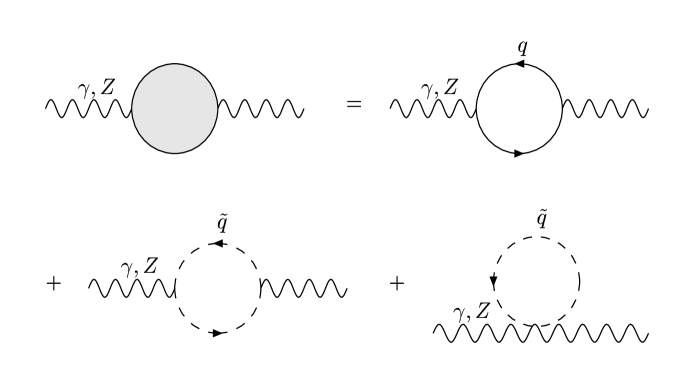
Figure 21: Top and bottom quark and squark contributions to the unrenormalized self-energy of $\gamma$ or $Z$

The gauge boson two–point functions can be written as $i[A_{GG}(p^{2})g^{\mu\nu}+B_{GG}(p^{2})p^{\mu}p^{\nu}]$ where $p$ is the external momentum and $GG=ZZ$, $\gamma\gamma$, or $Z\gamma$. The functions $A_{GG}$ and $B_{GG}$ depend on $p^{2}$ and represent the one–loop contributions to the gauge bosons self energies and mixing. For our purposes only $A_{GG}$ is relevant. We detail here the contribution to the gauge bosons self energies from top and bottom quarks and squarks, as shown in Fig. 21. We start with the $Z$–boson self energy. The contribution from top and bottom quarks is

$$\Big{[}A_{ZZ}(p^{2})\Big{]}^{tb} = {{N_{c}g^{2}}\over{32\pi^{2}c_{W}^{2}}}(m_{t}^{2}B_{0}^{ptt}+m_{b}^{2}B_{0}^{pbb})$$ (C.9)

$$- {{N_{c}g^{2}}\over{16\pi^{2}c_{W}^{2}}}({\textstyle{1\over 4}}-e_{t}s_{W}^{2}+2e_{t}^{2}s_{W}^{4})(4B_{22}^{ptt}-2A_{0}^{t}+p^{2}B_{0}^{ptt})$$

$$- {{N_{c}g^{2}}\over{16\pi^{2}c_{W}^{2}}}({\textstyle{1\over 4}}+e_{b}s_{W}^{2}+2e_{b}^{2}s_{W}^{4})(4B_{22}^{pbb}-2A_{0}^{b}+p^{2}B_{0}^{pbb})$$

where $A_{0}^{t}\equiv A_{0}(m_{t}^{2})$, $B_{22}^{ptt}\equiv B_{22}(p^{2};m_{t}^{2},m_{t}^{2})$, and similarly for $B_{0}$. The contribution from squarks is

$$\Big{[}A_{ZZ}(p^{2})\Big{]}^{\tilde{t}\tilde{b}} = {{N_{c}}\over{4\pi^{2}}}\sum_{i=1}^{2}\sum_{j=1}^{2}\left[\lambda_{Z\tilde{t}\tilde{t}}^{ij2}B_{22}^{p\tilde{t}_{i}\tilde{t}_{j}}+\lambda_{Z\tilde{b}\tilde{b}}^{ij2}B_{22}^{p\tilde{b}_{i}\tilde{b}_{j}}\right]$$ (C.10)

$$- {{N_{c}}\over{16\pi^{2}}}\sum_{i=1}^{2}\left[\lambda_{ZZ\tilde{t}\tilde{t}}^{ij}A_{0}^{\tilde{t}_{i}}+\lambda_{ZZ\tilde{b}\tilde{b}}^{ij}A_{0}^{\tilde{b}_{i}}\right]$$

where the couplings $\lambda_{Z\tilde{t}\tilde{t}}$ and $\lambda_{ZZ\tilde{t}\tilde{t}}$ are defined in Appendix A.

The photon self energy $A_{\gamma\gamma}$ receive contributions from top and bottom quarks:

$$\Big{[}A_{\gamma\gamma}(p^{2})\Big{]}^{tb}=-{{N_{c}e^{2}}\over{8\pi^{2}}}\bigg{[}e_{t}^{2}(4B_{22}^{ptt}-2A_{0}^{t}+p^{2}B_{0}^{ptt})+e_{b}^{2}(4B_{22}^{pbb}-2A_{0}^{b}+p^{2}B_{0}^{pbb})\bigg{]}$$ (C.11)

and from the top and bottom squarks:

$$\Big{[}A_{\gamma\gamma}(p^{2})\Big{]}^{\tilde{t}\tilde{b}}={{N_{c}e^{2}}\over{8\pi^{2}}}\sum_{i=1}^{2}\bigg{[}e_{t}^{2}(2B_{22}^{p\tilde{t}_{i}\tilde{t}_{i}}-A_{0}^{\tilde{t}_{i}})+e_{b}^{2}(2B_{22}^{p\tilde{b}_{i}\tilde{b}_{i}}-A_{0}^{\tilde{b}_{i}})\bigg{]}$$ (C.12)

where we take $e$ to be positive.

The top and bottom quarks contributions to the $Z-\gamma$ mixing is

$$\Big{[}A_{Z\gamma}(p^{2})\Big{]}^{tb}=-{{N_{c}ge}\over{16\pi^{2}c_{W}}}\bigg{[}e_{t}g_{V}^{t}(4B_{22}^{ptt}-2A_{0}^{t}+p^{2}B_{0}^{ptt})+e_{b}g_{V}^{b}(4B_{22}^{pbb}-2A_{0}^{b}+p^{2}B_{0}^{pbb})\bigg{]}$$ (C.13)

where $g_{V}^{t}={\textstyle{1\over 2}}(1-4e_{t}s_{W}^{2})$ and $g_{V}^{b}=-{\textstyle{1\over 2}}(1+4e_{b}s_{W}^{2})$. In the same way, the contributions from top and bottom squarks can be written as

$$\Big{[}A_{Z\gamma}(p^{2})\Big{]}^{\tilde{t}\tilde{b}}=-{{N_{c}e}\over{8\pi^{2}}}\sum_{i=1}^{2}\bigg{[}e_{t}\lambda_{Z\tilde{t}\tilde{t}}^{ii}(2B_{22}^{p\tilde{t}_{i}\tilde{t}_{i}}-A_{0}^{\tilde{t}_{i}})+e_{b}\lambda_{Z\tilde{b}\tilde{b}}^{ii}(2B_{22}^{p\tilde{b}_{i}\tilde{b}_{i}}-A_{0}^{\tilde{b}_{i}})\bigg{]}$$ (C.14)

and the couplings $Z$–squark–squark are in eq. A.60.

C3. Chargino Two–Point Functions

Figure 22: Feynman diagrams contributing to the unrenormalized chargino two–point functions.

In the approximation we are working on, i.e., including only top and bottom quarks and squarks in the loops, there are two types of one–loop graph which contribute to the chargino two–point functions, and they are displayed in Fig. 22. We use the notation for the sum of the Feynman diagrams contributing to the chargino two–point functions given in eq. (4.6). In this way, the graphs involving top quarks and bottom squarks are

$$\left[\Sigma_{\chi\chi}^{ij}(p^{2})\right]^{t\tilde{b}} = i{{N_{c}}\over{8\pi^{2}}}\sum_{k=1}^{2}\Bigg{\{}\bigg{[}{\lambda_{\tilde{b}t\chi}^{+kj}}^{*}\lambda_{\tilde{b}t\chi}^{-ki}(1-\gamma_{5})+{\lambda_{\tilde{b}t\chi}^{-kj}}^{*}\lambda_{\tilde{b}t\chi}^{+ki}(1+\gamma_{5})\bigg{]}m_{t}B_{0}^{pt\tilde{b}_{k}}$$ (C.15)

$$- \bigg{[}{\lambda_{\tilde{b}t\chi}^{+kj}}^{*}\lambda_{\tilde{b}t\chi}^{+ki}(1-\gamma_{5})+{\lambda_{\tilde{b}t\chi}^{-kj}}^{*}\lambda_{\tilde{b}t\chi}^{-ki}(1+\gamma_{5})\bigg{]}p_{\mu}\gamma^{\mu}B_{1}^{pt\tilde{b}_{k}}\Bigg{\}}$$

and for bottom quarks and top squarks we have

$$\left[\Sigma_{\chi\chi}^{ij}(p^{2})\right]^{b\tilde{t}} = -i{{N_{c}}\over{8\pi^{2}}}\sum_{k=1}^{2}\Bigg{\{}\bigg{[}\lambda_{\tilde{t}b\chi}^{-kj}{\lambda_{\tilde{t}b\chi}^{+ki}}^{*}(1+\gamma_{5})+\lambda_{\tilde{t}b\chi}^{+kj}{\lambda_{\tilde{t}b\chi}^{-ki}}^{*}(1-\gamma_{5})\bigg{]}m_{b}B_{0}^{pb\tilde{t}_{k}}$$ (C.16)

$$- \bigg{[}\lambda_{\tilde{t}b\chi}^{-kj}{\lambda_{\tilde{t}b\chi}^{-ki}}^{*}(1+\gamma_{5})+\lambda_{\tilde{t}b\chi}^{+kj}{\lambda_{\tilde{t}b\chi}^{+ki}}^{*}(1-\gamma_{5})\bigg{]}p_{\mu}\gamma^{\mu}B_{1}^{pb\tilde{t}_{k}}\Bigg{\}}$$

with the couplings given in eq. (A.61).

References

- [1] H.P. Nilles, Phys. Rep. 110, 1 (1984); H.E. Haber and G.L. Kane, Phys. Rep. 117, 75 (1985); R. Barbieri, Riv. Nuovo Cimento 11, 1 (1988).
- [2] H. Komatsu and J. Kubo, Phys. Lett. 162B, 379 (1985); R. Barbieri, G. Gamberini, G.F. Giudice, and G. Ridolfi, Phys. Lett. 195B, 500 (1987); M.S. Carena and C.E.M. Wagner, Phys. lett. 195B, 599 (1987); H. Konig, U. Ellwanger, and M.G. Schmidt, Z. Phys. C36, 715 (1987); A. Bartl, W. Majerotto, and N. Oshimo, Phys. Lett. B 216, 233 (1989); A. Bartl, S. Stippel, W. Majerotto, and N. Oshimo, Phys. Lett. B 233, 241 (1989); A. Bartl, W. Majerotto, N. Oshimo, and S. Stippel, Z. Phys. C47, 235 (1990); K. Hidaka and P. Ratcliffe, Phys. Lett. B 252, 476 (1990).
- [3] A. Bartl, H. Fraas, and W. Majerotto, Z. Phys. C30, 441 (1986); A. Bartl, H. Fraas, and W. Majerotto, Nucl. Phys. B278, 1 (1986); A. Bartl, H. Fraas, W. Majerotto, and B. Mosslacher, Z. Phys. C55, 257 (1992); M.H. Nous, M. El-Kishen, and T.A. El-Azem, Mod. Phys. Lett. A7, 1535 (1992); J. Feng and M. Strassler, Phys. Rev. D 51, 4661 (1995); J.L. Feng and M.J. Strassler, Phys. Rev. D 55, 1326 (1997); M.A. Díaz, Mod. Phys. Lett. A12, 307 (1997); J. Gluza and T. Wohrmann Phys. Lett. B408, 229 (1997); A.S. Belyaev and A.V. Gladyshev, Report No. JINR-E2-97-76, Mar 1997, (hep-ph/9703251).
- [4] J.F. Gunion et al., Int. J. Mod. Phys. A2, 1147 (1987); J.F. Gunion and H.E. Haber, Phys. Rev. D 37, 2515 (1988); H.E. Haber and D. Wyler, Nucl. Phys. B323, 267 (1989); Y. Kizukuri and N. Oshimo, Phys. Lett. B 220, 293 (1989); J.H. Reid, E.J.O. Gavin, and M.A. Samuel, Phys. Rev. D 49, 2382 (1994).
- [5] H. Baer and X. Tata, Report No. FSU-HEP-921222, Dec. 1992.
-
[6]
M. Díaz and S.F.King, Phys. Lett. B 349, 105 (1995);
M. Díaz and S.F.King, Phys. Lett. B 373, 100 (1996). - [7] ALEPH Collaboration (R. Barate et al.), Report No. CERN–PPE–97–128 (hep–ex/9710012), Sep. 1997, submitted to Z. Phys. C.
- [8] DELPHI Collaboration (P. Abreu et al.), Report No. CERN–PPE–97–107, Aug. 1997, submitted to Z. Phys. C.
- [9] L3 Collaboration (M. Acciarri et al.), Report No. CERN–PPE–97–130, Sep. 1997, submitted to Phys. Lett. B.
- [10] OPAL Collaboration (K. Ackerstaff et al.), Report No. CERN–PPE–97–083, (hep–ex/9708018), submitted to Z. Phys. C.
- [11] D. Pierce, A. Papadopoulos,Phys. Rev. D 50, 565 (1994).
- [12] G. Passarino and M. Veltman, Nucl. Phys. B 160, 151 (1979).
- [13] H. Haber and G. Kane, Phys. Rev. 117, 75 (1985).
- [14] J.F. Gunion and H.E. Haber, Nucl. Phys. B 272, 1 (1986); erratum-ibid. B 402, 567 (1993).