The Lamb Shift in Dimensional Regularisation

Abstract

We present a simple derivation of the Lamb shift using effective field theory techniques and dimensional regularisation.

Keywords: Effective Field Theories, NRQED, NRQCD, HQET.

PACS: 11.10.St, 12.20.-m, 12.39.Hg

The explanation of the Lamb shift [1] is one of the early applications of the quantised electromagnetic field [2]. Although many text books [3] contain detailed expositions on this effect, the conventional derivations are subtle and rather intrincated. In particular a careful separation of small and large momenta must be carried out at some stage of the calculation.

It has already been noticed [4] that modern techniques of effective field theory lead to a simpler derivation of the Lamb shift. The important point to be realised is that in non-relativistic bound states there is a hierarchy of well separated scales [5]. Namely, the mass of the particle which forms the bound state (hard), the typical relative momentum in the bound state (soft) and the typical energy of the bound state (ultrasoft). In ref. [6] counting rules were given to work out the size of a given NRQED diagram in the Coulomb gauge for soft and ultrasoft photons respectively. These rules were used in ref. [4] to obtain the Lamb shift $O(m\alpha^{5})$, which requires the matching of QED to NRQED at one loop. The calculations were done using a cut-off and a photon mass to regulate the UV divergencies in the effective theory and IR divergences in both theories respectively.

In this note we point out that a further step in clarity and simplicity is achieved by (i) matching NRQED to an effective theory for ultrasoft photons which we have called potential NRQED (pNRQED) [7] and (ii) using dimensional regularisation (DR) for both UV and IR divergences. Since we are interested in the physics at the ultrasoft scale, we may sequentially integrate out energies and momenta at the hard and soft scales. This is carried out by matching to suitable effective field theories. Integrating out the hard scale leads from QED to the celebrated NRQED. Integrating out the soft scale produces potential terms and leads from NRQED to pNRQED. In both cases the matching is most efficiently done in DR.

The matching from QED to NRQED at one loop for the bilinear term in fermions has been carried out using dimensional regularisation in [8] and for the four-fermion operators in [7]. Since we are interested in the interaction with a static source the infinite mass limit for the nucleus field is taken. Hence the only relevant terms at $O(m\alpha^{5})$ in the NRQED Lagrangian are the following.

$${\cal L}_{NRQED}= \psi^{\dagger}\Biggl{\{}iD^{0}+\,{{\bf D}^{2}\over 2m}+{{\bf D}^{4}\over 8m^{3}}+c_{F}\,g{{\bf\mbox{\boldmath$\sigma$}\cdot B}\over 2m}+c_{D}\,g{\left[{\bf\mbox{\boldmath$\nabla$}\cdot E}\right]\over 8m^{2}}$$

$$+ic_{S}\,g{{\bf\mbox{\boldmath$\sigma$}\cdot\left(D\times E-E\times D\right)}\over 8m^{2}}\Biggr{\}}\psi+N^{\dagger}iD^{0}N$$

$$-{1\over 4}d_{1}F_{\mu\nu}F^{\mu\nu}+{d_{2}\over m^{2}}F_{\mu\nu}D^{2}F^{\mu\nu}\,,$$

where $iD^{0}=i\partial_{0}-eA^{0}$ , $i{\bf D}=i{\mbox{\boldmath$\nabla$}}+e{\bf A}$ on the electron field $\psi$ and $iD^{0}=i\partial_{0}+eZA^{0}$ on the nucleus field. The matching coefficients read

$$c_{F} = 1+{\alpha\over 2\pi}\,,$$

$$c_{D} = 1+{\alpha\over\pi}\left({8\over 3}\log{m\over\mu}\right)\,,$$

$$c_{S} = 1+{\alpha\over\pi}\,,$$ (2)

$$d_{1} = 1-{\alpha\over 3\pi}\log m^{2}/\mu^{2}\,,$$

$$d_{2} = {\alpha\over 60\pi}\,.$$

The fact that only the terms displayed in (1) are relevant can be easily seen by drawing diagrams of one electron one nucleus irreducible Green function (i.e. diagrams which cannot be disconnected by cutting one electron and one nucleus line) and taking into account that the next relevant scale is $m\alpha$. For diagrams which cannot be disconnected by cutting a photon line the order of the leading contribution of each diagram is $m\alpha^{r+s+1}$, where $r$ is the number of $\alpha$ that appear explicitly in the diagram and $s$ the number of $1/m$ factors (which must be compensated by $m\alpha$ until we obtain dimensions of energy). For diagrams which can be disconnected by cutting a photon line there is an extra suppression if $n$ time derivatives act on this photon line. This is due to the fact that these time derivatives are only sensible to the typical energy. The extra suppression factor is $\alpha^{n}$. We should keep in mind however that a given diagram in NRQED in general contains subleading contributions in $\alpha$ as well [6]. On the contrary pNRQED will be specially designed in such a way that each term and diagram contributes to a single order in $\alpha$.

Before going on, let us briefly comment on $d_{1}$ in (1). This factor can be set to one by rescaling the photon field. The only effect this rescaling has in the effective Lagrangian is redefining the electric charge $e$. The redefined $e$ is the low energy electron charge which is the one actually measured in low energy experiments, namely the one whose value is $e^{2}/4\pi=\alpha\sim 1/137$. Therefore $d_{1}$ will be put to one from now on.

pNRQED must be regarded as an effective field theory where electron and photon energies and (relative) momentum $\sim m\alpha$ have been integrated out. It is important to realise that because both the energy and momentum we are integrating out are $\sim m\alpha$ we can use HQET (static) propagators for the electron field to carry out the matching. This allows to match NRQED and pNRQED at a given order of $1/m$ and $\alpha$. The pNRQED Lagrangian can be written down at two levels: (i) in terms of electron and nucleus fields and (ii) in terms of bound state wave function fields. The level (i) is suitable for the matching calculation whereas the level (ii) is more convenient for bound state calculations. In fact it is at this level where the order of each term becomes explicit. The pNRQED (i) Lagrangian is a functional of $\psi(t,{\bf x})$, $N(t,{\bf x})$ and ultrasoft photon fields $A_{\mu}(t,{\bf x})$, which also contains (potential) terms non-local in space. $A_{\mu}(t,{\bf x})$ being ultrasoft means that they must be multipole expanded about the position of the nucleus in the one electron one nucleon Green function. Recall that this is due to the fact that in a bound state ${\bf x}\sim 1/m\alpha$ whereas the typical energy and momentum scales for ultrasoft photons are $\sim m\alpha^{2}$.

The matching for the electron and nucleus bilinears is trivial since the related Green functions are blind to the relative momentum. Hence the terms bilinear in electron fields and the terms bilinear in nucleus fields in NRQED remain the same in pNRQED. The terms containing photon fields only also remain exactly the same in NRQED and pNRQED. However we should keep in mind that now they correspond to ultrasoft photons only. The matching of one electron one nucleus Green functions induces potential terms in pNRQED. Namely terms bilinear in the electron and nucleus fields which are local in time but non-local in space. If we use the Coulomb gauge, at the order we are interested in it is enough to calculate the above Green functions at zero energy and at some non-zero relative momentum ${\bf p}$. Indeed, if the photon fields in this Green function calculated from the pNRQED Lagrangian are multipole expanded, any loop gives zero in DR as we argue next. First of all there is no scale for the energy. Second, there is a scale for the momentum but both the HQET propagators and the (multipole expanded) transverse gluon propagators are insensitive to it. Hence all loops in pNRQED have no scale and can be put to zero in DR. Consequently the potential terms in pNRQED can be read off directly from the calculation in NRQED.

A word of caution is needed. Strictly speaking the procedure above is not complete: it misses off-shell photons of energy $\sim$ $m\alpha^{2}$ and momentum $\sim$ $m\alpha$. In particular, we miss the contribution of diagrams which can be disconnected by cutting a photon line when time derivatives appear in this line. In the Coulomb gauge such photons start playing a role at order $m\alpha^{7}$. However, if a covariant gauge is used longitudinal photons in that region start playing a role already at order $m\alpha^{4}$ and hence they must be taken into account to calculate the Lamb shift in those gauges. Anyway, the matching procedure can be refined so that the effect of such photons is included. We shall elaborate on this point elsewhere.

At the order we are interested in only the NRQED diagrams in Fig. 1 contribute to the matching. We obtain

$$L_{pNRQED}= \int d^{3}{\bf x}\Biggl{(}\psi^{\dagger}\Biggl{\{}iD^{0}+\,{{\bf D}^{2}\over 2m}+{{\bf D}^{4}\over 8m^{3}}\Biggr{\}}\psi+N^{\dagger}iD^{0}N-{1\over 4}F_{\mu\nu}F^{\mu\nu}\Biggr{)}$$

$$+\int d^{3}{\bf x}_{1}d^{3}{\bf x}_{2}N^{\dagger}N(t,{\bf x}_{2})\Biggl{(}{Z\alpha\over|{\bf x}_{1}-{\bf x}_{2}|}+{Ze^{2}\over m^{2}}\left(-{c_{D}\over 8}+4d_{2}\right)\delta^{3}({\bf x}_{1}-{\bf x}_{2})$$

$$+ic_{S}{Z\alpha\over 4m^{2}}{\mbox{\boldmath$\sigma$}}\cdot\left({{\bf x}_{1}-{\bf x}_{2}\over|{\bf x}_{1}-{\bf x}_{2}|^{3}}\times{\mbox{\boldmath$\nabla$}}\right)\Biggr{)}\psi^{\dagger}\psi(t,{\bf x}_{1})\,.$$

It is convenient to project the Lagrangian (at level (i)) above to the one electron one nucleus subspace and thus obtain the pNRQED Lagrangian at level (ii). This subspace is spanned by

$$\int d^{3}{\bf x}_{1}d^{3}{\bf x}_{2}\varphi({\bf x}_{1},{\bf x}_{2})\psi^{\dagger}({\bf x}_{1})N^{\dagger}({\bf x}_{2})|0\rangle\,,$$ (4)

where $|0\rangle$ is the subspace of the Fock space containing zero electrons and nuclei but an arbitrary number of ultrasoft photons. Since there are not spatial derivatives acting on ${\bf x}_{2}$ the nucleus can be approximated by a static source which may be taken at the origin. Then

$$\varphi({\bf x}_{1},{\bf x}_{2})=\varphi({\bf x}_{1})\delta^{3}({\bf x}_{2})\,.$$ (5)

The dynamics of $\varphi(t,{\bf x})$ is then described by the following Lagrangian

$$L_{pNRQED}=\int d^{3}{\bf x}\varphi^{\dagger}(t,{\bf x})\Biggl{(}i\partial_{0}-e(1-Z)A_{0}(t,{\bf 0})-ex^{i}\partial_{i}A_{0}(t,{\bf 0})+{{{\mbox{\boldmath$\nabla$}}}^{2}\over 2m}+{Z\alpha\over|{\bf x}|}$$

$$-ie{{\bf A}(t,{\bf 0})\cdot{{\mbox{\boldmath$\nabla$}}}\over m}+{{{\mbox{\boldmath$\nabla$}}}^{4}\over 8m^{3}}+{Ze^{2}\over m^{2}}\left(-{c_{D}\over 8}+4d_{2}\right)\delta^{3}({\bf x})+ic_{S}{Z\alpha\over 4m^{2}}{\mbox{\boldmath$\sigma$}}\cdot\left({{\bf x}\over|{\bf x}|^{3}}\times{\mbox{\boldmath$\nabla$}}\right)\Biggr{)}\varphi(t,{\bf x})$$

$$-\int d^{3}{\bf x}{1\over 4}F_{\mu\nu}F^{\mu\nu}\,,$$ (6)

where we have multipole expanded $A_{\mu}(t,{\bf x}_{1})$ about zero. Each term in this Lagrangian has a well defined size. $\partial_{i}$ acting on the electron field and $1/|{\bf x}|$ are $\sim m\alpha$. Space derivatives acting on $A_{\mu}(t,{\bf 0})$, time derivatives and $A_{\mu}(t,{\bf 0})$ itself are $\sim m\alpha^{2}$. The contribution of a given diagram to the energy is given by $m\alpha^{r+2s+p+2}$. $r$ is the number of explicit $\alpha$ in the diagram, $s$ the number of $1/m$ and $p$ the number of $x^{i}$ minus three times the number of $\delta^{3}({\bf x})$ minus the number of $1/|{\bf x}|$ minus the number of $\partial_{i}$. We have kept in (6) only the terms which are relevant to calculate the energy at $O(m\alpha^{5})$. There are more terms of the same size (e.g. $-ie({\bf x.\mbox{\boldmath$\nabla$}}{\bf A}(t,{\bf 0})){\bf.\mbox{\boldmath$\nabla$}}/m$) which however do not contribute to the energy at the desired order as it can be seen by counting the order of the diagrams in which they appear. (Dropping the term $-ex^{i}x^{j}\partial_{i}\partial_{j}A_{0}(t,{\bf 0})$ requires a more detailed analysis if a covariant gauge is to be used).

Gauge invariance can be checked order by order in this counting by introducing a gauge covariant field $S(t,{\bf x})$ as $\varphi(t,{\bf x})=\bigl{[}e^{ie\int_{{\bf 0}}^{{\bf x}}{\bf A}d{\bf x}}\bigr{]}S(t,{\bf x})$, such that it transforms $S(t,{\bf x})\rightarrow e^{-ie(Z-1)\theta(t,{\bf 0})}S(t,{\bf x})$. From this transformation it is clear that we should regard $S(t,{\bf x})$ like an ion field rather than an electron field. After multipole expanding at the desired order, we obtain an explicitly gauge invariant Lagrangian

$$L_{pNRQED}= \int d^{3}{\bf x}S^{\dagger}(t,{\bf x})\Biggl{(}i\partial_{0}-e(1-Z)A_{0}(t,{\bf 0})+e{\bf x}\cdot{\bf E}(t,{\bf 0})+{{{\mbox{\boldmath$\nabla$}}}^{2}\over 2m}+{Z\alpha\over|{\bf x}|}$$ (7)

$$+{{{\mbox{\boldmath$\nabla$}}}^{4}\over 8m^{3}}+{Ze^{2}\over m^{2}}\left(-{c_{D}\over 8}+4d_{2}\right)\delta^{3}({\bf x})+ic_{S}{Z\alpha\over 4m^{2}}{\mbox{\boldmath$\sigma$}}\cdot\left({{\bf x}\over|{\bf x}|^{3}}\times{\mbox{\boldmath$\nabla$}}\right)\Biggr{)}S(t,{\bf x})$$

$$-\int d^{3}{\bf x}{1\over 4}F_{\mu\nu}F^{\mu\nu}\,.$$

It is also interesting to notice that the same Lagrangian above can be obtained by using backwards the equation of motion in the first term of the second line in (6).

$$\int d^{4}x\varphi^{\dagger}i{e\over m}{\bf A}(t,{\bf 0})\cdot{\mbox{\boldmath$\nabla$}}\varphi=\int d^{4}x\varphi^{\dagger}ie{\bf A}(t,{\bf 0})\cdot\left[{\bf x},\hat{h}_{0}\right]\varphi=\int d^{4}x\varphi^{\dagger}e\partial_{0}{\bf A}(t,{\bf 0})\cdot{\bf x}\,\varphi\,,$$

where

$$\hat{h}_{0}=-{\mbox{\boldmath$\nabla$}^{2}\over 2m}-{Z\alpha\over|{\bf x}|}\,.$$ (9)

The Lamb shift receives contributions from the propagation of ultrasoft photons in the bound state. Notice that since the lagrangian of pNRQED (ii) is explicitly gauge invariant we can use any gauge to calculate with it. Still the Coulomb gauge continues to be advantageous. In this gauge $A_{0}(t,{\bf 0})$ can be dropped if we use DR since it only produces tadpoles. If a covariant gauge is used the propagation of $A_{0}(t,{\bf 0})$ must also be taken into account. In the Coulomb gauge at $O(m\alpha^{5})$ the ultrasoft photons contribute to the bound state energy only through the pNRQED diagram of Fig. 2. In order to calculate this contribution we consider the two point function

$$\Pi(q,{\bf x}):=\int dx^{0}e^{iqx^{0}}<T\{\varphi(0)\varphi^{\dagger}(x)\}>$$ (10)

when $q\rightarrow E_{n}$. We write

$$\Pi(q,{\bf x})={A_{n}+\delta A_{n}\over q-(E_{n}+\delta E_{n})}\sim{A_{n}+\delta A_{n}\over q-E_{n}}+{A_{n}\over q-E_{n}}\delta E_{n}{1\over q-E_{n}}\,.$$ (11)

$\Pi(q,{\bf x})$ must be calculated in $D$ dimensions. By introducing the complete set of eigenfunction of $\hat{h}_{0}$ in $D=4-\epsilon$ dimensions $\hat{h}_{0}\phi_{n}=E_{n}\phi_{n}$, we obtain

$$\Pi(q,{\bf x})\sim{i\phi_{n}(0)\phi_{n}^{\dagger}({\bf x})\over q-E_{n}}-{e^{2}}{i\phi_{n}(0)\over q-E_{n}}\sum_{m}\langle n|{\bf v}^{i}|m\rangle I_{ij}(q-E_{m})\langle m|{\bf v}^{j}|n\rangle{i\phi^{\dagger}_{n}({\bf x})\over q-E_{n}}\,,$$ (12)

where ${\bf v}=-i{\mbox{\boldmath$\nabla$}}/m$. We have then to calculate the following integral

$$I_{ij}(p)= \int{d^{D}k\over(2\pi)^{D}}{i\over k^{2}}\left(\delta^{ij}-{k^{i}k^{j}\over{{\bf k}}^{2}}\right){i\over p-k^{0}+i\eta}$$

$$= -ip{1\over 6\pi^{2}}\delta^{ij}\left({1\over\epsilon}+{1\over 2}\log{4\pi}+\log{\mu\over-p-i\eta}+{5\over 6}-{\gamma\over 2}-\log{2}\right)\,.$$

This integral is carried out by (i) first integrating over $k_{0}$ and then (ii) choosing a contour in the $|{\bf k}|$ complex plain which embraces the cut on the positive real axes and closes itself at infinity in such a way that the pole of the integrand is always left inside the contour. Notice that the divergent part of this integral is a polynomial. Before going on let us check that it can be absorbed by a counterterm in $L_{pNRQED}$. Indeed,

$$\delta^{US,local}E_{n}\sim \sum_{m}\langle n|{\bf v}|m\rangle\left(q-E_{m}\right)\langle m|{\bf v}|n\rangle=\langle n|{\bf v}\left(q-\hat{h}_{0}\right){\bf v}|n\rangle$$ (14)

$$= \langle n|\Big{(}{1\over 2}\left(q-\hat{h}_{0}\right){\bf v}^{2}+{1\over 2}{\bf v}^{2}\left(q-\hat{h}_{0}\right)-{1\over 2}\left[{\bf v}\left[{\bf v},q-\hat{h}_{0}\right]\right]\Big{)}|n\rangle\,.$$

In order to identify $\delta E_{n}$ the strict limit $q\rightarrow E_{n}$ must be taken and hence the first two terms in the last expression can be dropped. The remaining term is nothing but the $D-1$ dimensional Laplacian acting on the $D$ dimensional Coulomb potential which gives a $D-1$ dimensional $\delta$-function. Thus (14) reads

$$\delta^{US,local}E_{n}\sim\langle n|\left(-{Ze^{2}\over 2m^{2}}\delta^{D-1}({\bf x})\right)|n\rangle\,,$$ (15)

which can be absorbed by a counterterm in the second last term of $L_{pNRQED}$ in (6) and (7). Since we have used $\overline{MS}$ subtraction scheme in the matching we must use the same subtraction scheme here. Since there are no further divergences left the limit $D\rightarrow 4$ can be safely taken. Notice that this procedure avoids calculating explicitly $\phi_{n}$ and $E_{n}$ in $D$ dimensions. We finally obtain that the contribution to the energy given by the diagram in Fig. 2 is

$$\delta^{US}E_{n}= {2\over 3}{\alpha\over\pi}\Bigg{(}\left(\log{\mu\over m}+{5\over 6}-\log{2}\right)\left({Ze^{2}\over 2}\right){|\phi_{n}({\bf 0})|^{2}\over m^{2}}$$

$$-\sum_{m\not=n}|\langle n|{\bf v}|m\rangle|^{2}\left(E_{n}-E_{m}\right)\log{m\over|E_{n}-E_{m}|}\Bigg{)}\,.$$

From the imaginary part of (13) we also obtain the total width

$$\Gamma_{n}=\sum_{m<n}{4\over 3}\alpha|\langle n|{\bf v}|m\rangle|^{2}\left(E_{n}-E_{m}\right)\,.$$ (17)

The remaining contribution at $O(m\alpha^{5})$ arises from the above mentioned potential terms in (6) and (7). It reads

$$\delta^{S}E_{n}= \delta^{S,K}E_{n}+\delta^{S,\delta}E_{n}+\delta^{S,S}E_{n}\,,$$

$$\delta^{S,K}E_{n}= -{1\over 8m^{3}}\langle nlj|\mbox{\boldmath$\nabla$}^{4}|nlj\rangle\,,$$

$$\delta^{S,\delta}E_{n}= {Ze^{2}\over m^{2}}\left({c_{D}\over 8}-4d_{2}\right)|\phi_{n}({\bf 0})|^{2}\,,$$

$$\delta^{S,S}E_{n}= c_{S}{Z\alpha\over 4m^{2}}\left(j(j+1)-l(l+1)-{3\over 4}\right)\langle nlj|{1\over{\bf x}^{3}}|nlj\rangle$$

($|n\rangle=|nlj\rangle$). Thus the correction to the bound state energy $\delta E_{n}$ up to $m\alpha^{5}$ included is obtained by adding up the soft and ultrasoft contributions

$$\delta E_{n}=\delta^{S}E_{n}+\delta^{US}E_{n}\,,$$ (19)

which agrees with the well known result. Recall that the hard contributions are encoded in $c_{D}$, $c_{S}$ and $d_{2}$. Notice also that the subtraction point dependences of $\delta^{S,\delta}E_{n}$ (in $c_{D}$) and $\delta^{US}E_{n}$ cancel out, as they should. However we should stress that in order to obtain the finite pieces right, it is necessary that the same subtraction scheme, namely $\overline{MS}$, which has been used in the matching be used in the calculations of pNRQED.

In summary we have presented a simple and complete derivation of the Lamb shift based on modern EFT techniques and dimensional regularisation. The derivation goes through two EFTs, namely NRQED and pNRQED, so that at any stage it becomes clear which terms and diagrams are to be considered to carry out a calculation at the desired order. The formulation of pNRQED, namely an effective field theory for ultrasof photons, has received quite some attention lately [6, 9]. In ref. [7] the matching from NRQED (NRQCD) to pNRQED (pNRQCD) was outlined and the pNRQED and pNRQCD Lagrangians for positronium and quarkonium were presented. Here we have worked out the pNRQED Lagrangian for Hydrogen-like atoms and presented its first application. Gauge invariance is manifest in the two EFTs. This is particularly remarkable in pNRQED, if we take into account that most of the previous attempts to deal with ultrasoft photons were strongly based on the Coulomb gauge. Last but not least DR allows to regulate both UV and IR divergences in a manifestly gauge invariant way (unlike the photon mass) and makes the matching calculations straightforward. These techniques are most promising when applied to bound states of heavy quarkonia in QCD [7].

Caption1. The first diagram is the Coulomb potential. The circle is the vertex proportional to $c_{D}$, the square to $c_{S}$ (spin dependent) and the dashed dot to $d_{1}$ (the vacuum polarization). The dashed, solid and double lines are the static photon, electron and nucleus propagators respectively.

Caption2. The thick line and wavy line are the ion and transverse photon propagators respectively.

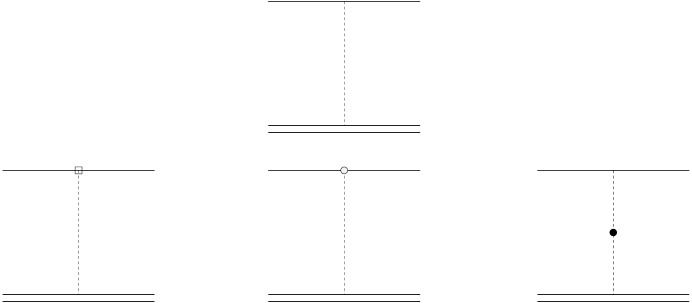
Figure 1:

Figure 2:

References

- [1] W.E. Lamb and R.C. Retherford, Phys. Rev. 72 (1947) 241.
- [2] H.A. Bethe, Phys. Rev. 72 (1947) 339.
- [3] C. Itzykson and J.-B. Zuber, Quantum Field Theory (McGraw-Hill, 1980).
- [4] P. Labelle and S.M. Zebarjad, Derivation of the Lamb Shift Using an Effective Field Theory, McGill-96/41, hep-ph/9611313.
- [5] W.E. Caswell and G.P. Lepage, Phys. Lett. B167 (1986) 437.
- [6] P. Labelle, Effective Field Theories for QED Bound States: Extending Nonrelativistic QED to Study Retardation Effects, McGill-96/33, hep-ph/9608491.
- [7] A. Pineda and J. Soto, Effective field Theory for ultrasoft momenta in NRQCD and NRQED, to be published in the proceedings of QCD97: 25th Anniversary of QCD, Montpellier, France, 3-9 July 1997, UB-ECM-PF 97/17, hep-ph/9707481.
- [8] A.V. Manohar, Phys. Rev. D56 (1997) 230.
- [9] I.Z. Grinstein and I.Z. Rothstein, Phys. Rev. D57 (1998) 78. M. Luke and A.V. Manohar, Phys. Rev. D55 (1997) 4129. M. Luke and M.J. Savage, Power counting in dimensionally regulated NRQCD, UTPT-97-12, hep-ph/9707313.