PRECISION TESTS OF THE STANDARD MODEL

Precision measurements of electroweak observables provide stringent tests of the Standard Model structure and an accurate determination of its parameters. An overview of the present experimental status is presented.

FTUV/97-45
IFIC/97-46
November 1997

1 Introduction

The Standard Model (SM) constitutes one of the most successful achievements in modern physics. It provides a very elegant theoretical framework, which is able to describe all known experimental facts in particle physics. A detailed description of the SM and its impressive phenomenological success can be found in Refs. 1 and 2, which discuss the electroweak and strong sectors, respectively.

The high accuracy achieved by the most recent experiments allows to make stringent tests of the SM structure at the level of quantum corrections. The different measurements complement each other in their different sensitivity to the SM parameters. Confronting these measurements with the theoretical predictions, one can check the internal consistency of the SM framework and determine its parameters.

These lectures provide an overview of our present experimental knowledge on the electroweak couplings. A brief description of some classical QED tests is presented in Section 2. The leptonic couplings of the $W^{\pm}$ bosons are analyzed in Section 3, where the tests on lepton universality and the Lorentz structure of the $l^{-}\to\nu_{l}l^{\prime-}\bar{\nu}_{l^{\prime}}$ transition amplitudes are discussed. Section 4 describes the status of the neutral–current sector, using the latest experimental results reported by LEP and SLD. Some summarizing comments are finally given in Section 5. I have skipped completely the analysis of the $W^{\pm}$ couplings to the charged quark currents; a rather exhaustive description of the existing constraints on the quark–mixing matrix and the present status of CP–violation phenomena has been given in Refs. 3 and 4.

2 QED

A general description of the electromagnetic coupling of a spin–$\frac{1}{2}$ charged lepton to the virtual photon involves three different form factors:

$$T[l\bar{l}\gamma^{*}]=e\,\varepsilon_{\mu}(q)\,\bar{l}\left[F_{1}(q^{2})\gamma^{\mu}+i{F_{2}(q^{2})\over 2m_{l}}\sigma^{\mu\nu}q_{\nu}+{F_{3}(q^{2})\over 2m_{l}}\sigma^{\mu\nu}\gamma_{5}q_{\nu}\right]l\ ,$$ (1)

where $q^{\mu}$ is the photon momentum. Owing to the conservation of the electric charge, $F_{1}(0)=1$. At $q^{2}=0$, the other two form factors reduce to the lepton magnetic dipole moment $\mu_{l}\equiv(e/2m_{l})\,(g_{l}/2)=e(1+F_{2}(0))/2m_{l}$, and electric dipole moment $d_{l}=eF_{3}(0)/2m_{l}$.

The $F_{i}(q^{2})$ form factors are sensitive quantities to a possible lepton substructure. Moreover, $F_{3}(q^{2})$ violates $T$ and $P$ invariance; thus, the electric dipole moments, which vanish in the SM, constitute a good probe of CP violation. Owing to their chiral–changing structure, the magnetic and electric dipole moments may provide important insights on the mechanism responsible for mass generation. In general, one expects $\!{}^{{\bf?}}$ that a fermion of mass $m_{f}$ (generated by physics at some scale $M\gg m_{f}$) will have induced dipole moments proportional to some power of $m_{f}/M$.

The measurement of the $e^{+}e^{-}\to l^{+}l^{-}$ cross-section has been used to test the universality of the leptonic QED couplings. At low energies, where the $Z$ contribution is small, the deviations from the QED prediction are usually parameterized through

$$\sigma(e^{+}e^{-}\to l^{+}l^{-})\,=\,\sigma_{\mbox{\rm\scriptsize QED}}\,\left(1\mp{s\over s-\Lambda_{\pm}^{2}}\right)^{2}.$$ (2)

The cut-off parameters $\Lambda_{\pm}$ characterize the validity of QED and measure the point-like nature of the leptons. From PEP and PETRA data, one finds $\!{}^{{\bf?}}$: $\Lambda_{+}(e)>435$ GeV, $\Lambda_{-}(e)>590$ GeV, $\Lambda_{+}(\mu)>355$ GeV, $\Lambda_{-}(\mu)>265$ GeV, $\Lambda_{+}(\tau)>285$ GeV and $\Lambda_{-}(\tau)>246$ GeV (95% CL), which correspond to upper limits on the lepton charge radii of about $10^{-3}$ fm.

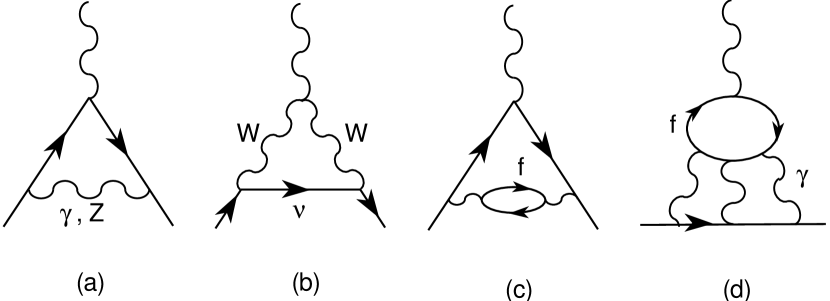
Figure 1: Some Feynman diagrams contributing to $a_{l}$.

The most stringent QED test comes from the high–precision measurements of the $e$ and $\mu$ anomalous magnetic moments $\!{}^{{\bf?},{\bf?},{\bf?},{\bf?},{\bf?},{\bf?},{\bf?},{\bf?},{\bf?},{\bf?},{\bf?},{\bf?}}$ $a_{l}\equiv(g_{l}-2)/2$:

$$a_{e} = \left\{\begin{array}[]{cc}(115\,965\,214.0\pm 2.8)\times 10^{-11}&(\mbox{\rm Theory})\\ (115\,965\,219.3\pm 1.0)\times 10^{-11}&(\mbox{\rm Experiment})\end{array}\,,\right.$$ (5)

$$a_{\mu} = \left\{\begin{array}[]{cc}(1\,165\,917.1\pm 1.0)\times 10^{-9}&(\mbox{\rm Theory})\\ (1\,165\,923.0\pm 8.4)\times 10^{-9}&(\mbox{\rm Experiment})\end{array}\,.\right.$$ (8)

The impressive agreement between theory and experiment (at the level of the ninth digit for $a_{e}$) promotes QED to the level of the best theory ever build by the human mind to describe nature. Hypothetical new–physics effects are constrained to the ranges $|\delta a_{e}|<1.1\times 10^{-10}$ and $|\delta a_{\mu}|<2.2\times 10^{-8}$ (95% CL).

To a measurable level, $a_{e}$ arises entirely from virtual electrons and photons; these contributions are known $\!{}^{{\bf?}}$ to $O(\alpha^{4})$. The sum of all other QED corrections, associated with higher–mass leptons or intermediate quarks, only amounts to $+(0.4366\pm 0.0042)\times 10^{-11}$, while the weak interaction effect is a tiny $+0.0030\times 10^{-11}$; these numbers $\!{}^{{\bf?}}$ are well below the present experimental precision. The theoretical error is dominated by the uncertainty in the input value of the electromagnetic coupling $\alpha$. In fact, turning things around, one can use $a_{e}$ to make the most precise determination of the fine structure constant $\!{}^{{\bf?}}$:

$$\alpha^{-1}=137.03599993\pm 0.00000052\,.$$ (9)

The resulting accuracy is one order of magnitude better than the usually quoted value $\!{}^{{\bf?}}$ $\alpha^{-1}=137.0359895\pm 0.0000061$.

The anomalous magnetic moment of the muon is sensitive to virtual contributions from heavier states; compared to $a_{e}$, they scale as $m_{\mu}^{2}/m_{e}^{2}$. The main theoretical uncertainty on $a_{\mu}$ has a QCD origin. Since quarks have electric charge, virtual quark–antiquark pairs can be created by the photon leading to the so–called hadronic vacuum polarization corrections to the photon propagator (Figure 1.c). Owing to the non-perturbative character of QCD at low energies, the light–quark contribution cannot be reliably calculated at present; fortunately, this effect can be extracted from the measurement of the cross-section $\sigma(e^{+}e^{-}\to\mbox{\rm hadrons})$ at low energies, and from the invariant–mass distribution of the final hadrons in $\tau$ decays $\!{}^{{\bf?}}$. The large uncertainties of the present data are the dominant limitation to the achievable theoretical precision on $a_{\mu}$. It is expected that this will be improved at the DA$\Phi$NE $\Phi$ factory, where an accurate measurement of the hadronic production cross-section in the most relevant kinematical region is expected $\!{}^{{\bf?}}$. Additional QCD uncertainties stem from the (smaller) light–by–light scattering contributions, where four photons couple to a light–quark loop (Figure 1.d); these corrections are under active investigation at present $\!{}^{{\bf?},{\bf?},{\bf?},{\bf?},{\bf?}}$.

The improvement of the theoretical $a_{\mu}$ prediction is of great interest in view of the new E821 experiment $\!{}^{{\bf?}}$, presently running at Brookhaven, which aims to reach a sensitivity of at least $4\times 10^{-10}$, and thereby observe the contributions from virtual $W^{\pm}$ and $Z$ bosons $\!{}^{{\bf?},{\bf?},{\bf?}}$ ($\delta a_{\mu}|_{\mbox{\rm\scriptsize weak}}\sim 15\times 10^{-10}$). The extent to which this measurement could provide a meaningful test of the electroweak theory depends critically on the accuracy one will be able to achieve pinning down the QCD corrections.

Experimentally, very little is known about $a_{\tau}$ since the spin precession method used for the lighter leptons cannot be applied due to the very short lifetime of the $\tau$. The effect is however visible in the $e^{+}e^{-}\to\tau^{+}\tau^{-}$ cross-section. The limit $|a_{\tau}|<0.023$ (95% CL) has been derived $\!{}^{{\bf?}}$ from PEP and PETRA data. This limit actually probes the corresponding form factor $F_{2}(s)$ at $s\sim 35$ GeV. A more direct bound at $q^{2}=0$ has been extracted $\!{}^{{\bf?}}$ from the decay $Z\to\tau^{+}\tau^{-}\gamma$:

$$|a_{\tau}|<0.049\qquad(90\%\,\mbox{\rm CL})\,.$$ (10)

A better, but more model–dependent, limit has been obtained $\!{}^{{\bf?}}$ from the $Z\to\tau^{+}\tau^{-}$ decay width: $-0.004<a_{\tau}<0.006$.

In the SM the overall value of $a_{\tau}$ is dominated by the second order QED contribution $\!{}^{{\bf?}}$, $a_{\tau}\approx\alpha/2\pi$. Including QED corrections up to O($\alpha^{3}$), hadronic vacuum polarization contributions and the corrections due to the weak interactions (which are a factor 380 larger than for the muon), the tau anomalous magnetic moment has been estimated to be $\!{}^{{\bf?},{\bf?}}$

$$a_{\tau}\big{|}_{\mbox{\rm\scriptsize th}}\,=\,(1.1773\pm 0.0003)\times 10^{-3}\,.$$ (11)

So far, no evidence has been found for any CP–violation signature in the lepton sector. The present limits on the leptonic electric dipole moments are $\!{}^{{\bf?},{\bf?}}$:

$$d_{e}\,=\,(-0.27\pm 0.83)\times 10^{-26}\,e\,\mbox{\rm cm},$$

$$d_{\mu}\,=\,(3.7\pm 3.4)\times 10^{-19}\,e\,\mbox{\rm cm},$$ (12)

$$|d_{\tau}|\,<\,2.7\times 10^{-16}\,e\,\mbox{\rm cm}\qquad(90\%\,\mbox{\rm CL})\,.$$

3 Charged–Current Couplings

In the SM, the charged–current interactions are governed by an universal coupling $g$:

$${\cal L}_{\mbox{\rm\scriptsize CC}}={g\over 2\sqrt{2}}\,W^{\dagger}_{\mu}\,\left[\sum_{ij}\,\bar{u}_{i}\gamma^{\mu}(1-\gamma_{5})V_{ij}d_{j}\,+\,\sum_{l}\,\bar{\nu}_{l}\gamma^{\mu}(1-\gamma_{5})l\right]\,+\,\mbox{\rm h.c.}\;.$$ (13)

In the original basis of weak eigenstates quarks and leptons have identical interactions. The diagonalization of the fermion masses gives rise to the unitary quark mixing matrix $V_{ij}$, which couples any up–type quark with all down–type quarks. For massless neutrinos, the analogous leptonic mixing matrix can be eliminated by a redefinition of the neutrino fields. The lepton flavour is then conserved in the minimal SM without right–handed neutrinos.

3.1 $\mu^{-}\to e^{-}\bar{\nu}_{e}\nu_{\mu}$

Figure 2: $\mu$–decay diagram.        Figure 3: $\tau$–decay diagram.

The simplest flavour–changing process is the leptonic decay of the muon, which proceeds through the $W$–exchange diagram shown in Figure 3. The momentum transfer carried by the intermediate $W$ is very small compared to $M_{W}$. Therefore, the vector–boson propagator reduces to a contact interaction,

$${-g_{\mu\nu}+q_{\mu}q_{\nu}/M_{W}^{2}\over q^{2}-M_{W}^{2}}\quad\;\stackrel{{\scriptstyle q^{2}\ll M_{W}^{2}}}{{\,\longrightarrow\,}}\quad\;{g_{\mu\nu}\over M_{W}^{2}}\,.$$ (14)

The decay can then be described through an effective local 4–fermion Hamiltonian,

$${\cal H}_{\mbox{\rm\scriptsize eff}}\,=\,{G_{F}\over\sqrt{2}}\left[\bar{e}\gamma^{\alpha}(1-\gamma_{5})\nu_{e}\right]\,\left[\bar{\nu}_{\mu}\gamma_{\alpha}(1-\gamma_{5})\mu\right]\,,$$ (15)

where

$${G_{F}\over\sqrt{2}}={g^{2}\over 8M_{W}^{2}}$$ (16)

is called the Fermi coupling constant. $G_{F}$ is fixed by the total decay width,

$${1\over\tau_{\mu}}\,=\,\Gamma(\mu^{-}\to e^{-}\bar{\nu}_{e}\nu_{\mu})\,=\,{G_{F}^{2}m_{\mu}^{5}\over 192\pi^{3}}\,\left(1+\delta_{\mbox{\rm\scriptsize RC}}\right)\,f\left(m_{e}^{2}/m_{\mu}^{2}\right)\,,$$ (17)

where $\,f(x)=1-8x+8x^{3}-x^{4}-12x^{2}\ln{x}$, and

$$(1+\delta_{\mbox{\rm\scriptsize RC}})=\left[1+{\alpha(m_{\mu})\over 2\pi}\left({25\over 4}-\pi^{2}\right)\right]\,\left[1+{3\over 5}{m_{\mu}^{2}\over M_{W}^{2}}-2{m_{e}^{2}\over M_{W}^{2}}\right]=0.9958\,$$ (18)

takes into account the leading higher–order corrections $\!{}^{{\bf?},{\bf?}}$. The measured lifetime $\!{}^{{\bf?}}$, $\tau_{\mu}=(2.19703\pm 0.00004)\times 10^{-6}$ s, implies the value

$$G_{F}\,=\,(1.16639\pm 0.00002)\times 10^{-5}\>\mbox{\rm GeV}^{-2}\,\approx\,{1\over(293\>\mbox{\rm GeV})^{2}}\,.$$ (19)

3.2 $\tau$ Decay

The decays of the $\tau$ proceed through the same $W$–exchange mechanism as the leptonic $\mu$ decay. The only difference is that several final states are kinematically allowed: $\tau^{-}\to\nu_{\tau}e^{-}\bar{\nu}_{e}$, $\tau^{-}\to\nu_{\tau}\mu^{-}\bar{\nu}_{\mu}$, $\tau^{-}\to\nu_{\tau}d\bar{u}$ and $\tau^{-}\to\nu_{\tau}s\bar{u}$. Owing to the universality of the $W$–couplings, all these decay modes have equal amplitudes (if final fermion masses and QCD interactions are neglected), except for an additional $N_{C}|V_{ui}|^{2}$ factor ($i=d,s$) in the semileptonic channels, where $N_{C}=3$ is the number of quark colours. Making trivial kinematical changes in Eq. (17), one easily gets the lowest–order prediction for the total $\tau$ decay width:

$${1\over\tau_{\tau}}\equiv\Gamma(\tau)\approx\Gamma(\mu)\left({m_{\tau}\over m_{\mu}}\right)^{5}\left\{2+N_{C}\left(|V_{ud}|^{2}+|V_{us}|^{2}\right)\right\}\approx{5\over\tau_{\mu}}\left({m_{\tau}\over m_{\mu}}\right)^{5}.$$ (20)

From the measured muon lifetime, one has then $\tau_{\tau}\approx 3.3\times 10^{-13}$ s, to be compared with the experimental value $\!{}^{{\bf?},{\bf?}}$ $\tau_{\tau}^{\mbox{\rm\scriptsize exp}}=(2.900\pm 0.012)\times 10^{-13}$ s.

Table 1: Experimental values $\!{}^{{\bf?}}$ of some basic $\tau$ decay branching fractions.

$B_{\tau\to e}$	$(17.80\pm 0.08)\%$
$B_{\tau\to\mu}$	$(17.30\pm 0.10)\%$
$R_{\tau}^{B}\equiv(1-B_{\tau\to e}-B_{\tau\to\mu})/B_{\tau\to e}$	$3.646\pm 0.022$
Br($\tau^{-}\to\nu_{\tau}\pi^{-}$)	$(11.07\pm 0.18)\%$
Br($\tau^{-}\to\nu_{\tau}K^{-}$)	$(0.71\pm 0.05)\%$

The branching ratios into the different decay modes are predicted to be:

$$B_{\tau\to l}\equiv\mbox{\rm Br}(\tau^{-}\to\nu_{\tau}l^{-}\bar{\nu}_{l})\approx{1\over 5}=20\%\ ,$$

$$R_{\tau}\equiv{\Gamma(\tau\to\nu_{\tau}+\mbox{\rm hadrons})\over\Gamma(\tau^{-}\to\nu_{\tau}e^{-}\bar{\nu}_{e})}\approx N_{C}\,,$$ (21)

in good agreement with the measured numbers $\!{}^{{\bf?}}$, given in Table 1. Our naive predictions only deviate from the experimental results by about 20%. This is the expected size of the corrections induced by the strong interactions between the final quarks, that we have neglected. Notice that the measured $\tau$ hadronic width provides strong evidence for the colour degree of freedom.

The pure leptonic decays $\tau^{-}\to e^{-}\bar{\nu}_{e}\nu_{\tau},\mu^{-}\bar{\nu}_{\mu}\nu_{\tau}$ are theoretically understood at the level of the electroweak radiative corrections $\!{}^{{\bf?}}$. The corresponding decay widths are given by Eqs. (17) and (18), making the appropriate changes for the masses of the initial and final leptons.

Using the value of $G_{F}$ measured in $\mu$ decay, Eq. (17) provides a relation between the $\tau$ lifetime and the leptonic branching ratios $\!{}^{{\bf?}}$:

$$B_{\tau\to e}={B_{\tau\to\mu}\over 0.972564\pm 0.000010}={\tau_{\tau}\over(1.6321\pm 0.0014)\times 10^{-12}\,\mbox{\rm s}}\,.$$ (22)

The errors reflect the present uncertainty of $0.3$ MeV in the value of $m_{\tau}$.

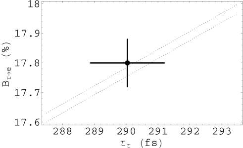
Figure 4: Relation between $B_{\tau\to e}$ and $\tau_{\tau}$. The dotted band corresponds to Eq. (22).

The predicted $B_{\tau\to\mu}/B_{\tau\to e}$ ratio is in perfect agreement with the measured value $B_{\tau\to\mu}/B_{\tau\to e}=0.972\pm 0.007$. As shown in Figure 4, the relation between $B_{\tau\to e}$ and $\tau_{\tau}$ is also well satisfied by the present data. Notice, that this relation is very sensitive to the value of the $\tau$ mass [$\Gamma(\tau^{-}\to l^{-}\bar{\nu}_{l}\nu_{\tau})\propto m_{\tau}^{5}$]. The experimental precision (0.4%) is already approaching the level where a possible non-zero $\nu_{\tau}$ mass could become relevant; the present bound $\!{}^{{\bf?}}$ $m_{\nu_{\tau}}<18.2$ MeV (95% CL) only guarantees that such effect is below 0.08%.

3.3 Semileptonic Decays

Semileptonic decays such as $\tau^{-}\to\nu_{\tau}P^{-}$ or $P^{-}\to l^{-}\bar{\nu}_{l}$ [$P=\pi,K$] can be predicted in a similar way. The effects of the strong interaction are contained in the so–called decay constants $f_{P}$, which parameterize the hadronic matrix element of the corresponding weak current:

$$\begin{array}[]{ccc}\langle\pi^{-}(p)|\bar{d}\gamma^{\mu}\gamma_{5}u|0\rangle&\equiv&-i\sqrt{2}f_{\pi}p^{\mu}\,,\\ \langle K^{-}(p)|\bar{s}\gamma^{\mu}\gamma_{5}u|0\rangle&\equiv&-i\sqrt{2}f_{K}p^{\mu}\,.\end{array}$$ (23)

Taking appropriate ratios of different semileptonic decay widths involving the same meson $P$, the dependence on the decay constants factors out. Therefore, those ratios can be predicted rather accurately:

$$R_{\pi\to e/\mu} \!\!\!\equiv \!\!\!{\Gamma(\pi^{-}\to e^{-}\bar{\nu}_{e})\over\Gamma(\pi^{-}\to\mu^{-}\bar{\nu}_{\mu})}\,=\,{m_{e}^{2}(1-m_{e}^{2}/m_{\pi}^{2})^{2}\over m_{\mu}^{2}(1-m_{\mu}^{2}/m_{\pi}^{2})^{2}}\,(1+\delta R_{\pi\to e/\mu})$$

$$\!\!\!= \!\!\!(1.2351\pm 0.0005)\times 10^{-4},$$

$$R_{\tau/\pi} \!\!\!\equiv \!\!\!{\Gamma(\tau^{-}\to\nu_{\tau}\pi^{-})\over\Gamma(\pi^{-}\to\mu^{-}\bar{\nu}_{\mu})}\,=\,{m_{\tau}^{3}\over 2m_{\pi}m_{\mu}^{2}}{(1-m_{\pi}^{2}/m_{\tau}^{2})^{2}\over(1-m_{\mu}^{2}/m_{\pi}^{2})^{2}}\left(1+\delta R_{\tau/\pi}\right)$$ (24)

$$\!\!\!= \!\!\!9774\pm 15\,,$$

$$R_{\tau/K} \!\!\!\equiv \!\!\!{\Gamma(\tau^{-}\to\nu_{\tau}K^{-})\over\Gamma(K^{-}\to\mu^{-}\bar{\nu}_{\mu})}\,=\,{m_{\tau}^{3}\over 2m_{K}m_{\mu}^{2}}{(1-m_{K}^{2}/m_{\tau}^{2})^{2}\over(1-m_{\mu}^{2}/m_{K}^{2})^{2}}\left(1+\delta R_{\tau/K}\right)$$

$$\!\!\!= \!\!\!480.4\pm 1.1\,,$$

where $\delta R_{\pi\to e/\mu}=-(3.76\pm 0.04)\%$, $\delta R_{\tau/\pi}=(0.16\pm 0.14)\%$ and $\delta R_{\tau/K}=(0.90\pm 0.22)\%$ are the computed $\!{}^{{\bf?},{\bf?}}$ radiative corrections. These predictions are in excellent agreement with the measured ratios $\!{}^{{\bf?},{\bf?},{\bf?},{\bf?}}$: $R_{\pi\to e/\mu}=(1.2310\pm 0.0037)\times 10^{-4}$, $R_{\tau/\pi}=9937\pm 166$ and $R_{\tau/K}=477\pm 34$.

3.4 Universality Tests

Table 2: Present constraints on $|g_{\mu}/g_{e}|$.

	$|g_{\mu}/g_{e}|$
$B_{\tau\to\mu}/B_{\tau\to e}$	$0.9997\pm 0.0037$
$R_{\pi\to e/\mu}$	$1.0017\pm 0.0015$
$\sigma\cdot B_{W\to\mu/e}$   ($p\bar{p}$)	$0.98\pm 0.03$
$B_{W\to\mu/e}$ (LEP2)	$0.92\pm 0.08$

Table 3: Present constraints on $|g_{\tau}/g_{\mu}|$.

	$|g_{\tau}/g_{\mu}|$
$B_{\tau\to e}\tau_{\mu}/\tau_{\tau}$	$1.0008\pm 0.0030$
$R_{\tau/\pi}$	$1.008\pm 0.008$
$R_{\tau/K}$	$0.997\pm 0.035$
$\sigma\cdot B_{W\to\tau/\mu}$   ($p\bar{p}$)	$1.02\pm 0.05$
$B_{W\to\tau/\mu}$ (LEP2)	$1.18\pm 0.11$

All these measurements can be used to test the universality of the $W$ couplings to the leptonic charged currents. Allowing the coupling $g$ in Eq. (13) to depend on the considered lepton flavour (i.e. $g_{e}$, $g_{\mu}$, $g_{\tau}$), the ratios $B_{\tau\to\mu}/B_{\tau\to e}$ and $R_{\pi\to e/\mu}$ constrain $|g_{\mu}/g_{e}|$, while $B_{\tau\to e}/\tau_{\tau}$ and $R_{\tau/P}$ provide information on $|g_{\tau}/g_{\mu}|$. The present results are shown in Tables 3 and 3, together with the values obtained from the comparison of the $\sigma\cdot B$ partial production cross-sections for the various $W^{-}\to l^{-}\bar{\nu}_{l}$ decay modes at the $p\bar{p}$ colliders $\!{}^{{\bf?}}$, and from the most recent LEP2 measurements of the leptonic $W^{\pm}$ branching ratios $\!{}^{{\bf?}}$.

Although the direct constraints from the measured $W^{-}\to l^{-}\bar{\nu}_{l}$ branching ratios are meager, the indirect information obtained in $W^{\pm}$–mediated decays provides stringent tests of the $W^{\pm}$ interactions. The present data verify the universality of the leptonic charged–current couplings to the 0.15% ($\mu/e$) and 0.30% ($\tau/\mu$) level. The precision of the most recent $\tau$–decay measurements is becoming competitive with the more accurate $\pi$–decay determination. It is important to realize the complementarity of the different universality tests. The pure leptonic decay modes probe the charged–current couplings of a transverse $W$. In contrast, the decays $\pi/K\to l\bar{\nu}$ and $\tau\to\nu_{\tau}\pi/K$ are only sensitive to the spin–0 piece of the charged current; thus, they could unveil the presence of possible scalar–exchange contributions with Yukawa–like couplings proportional to some power of the charged–lepton mass. One can easily imagine new physics scenarios which would modify differently the two types of leptonic couplings $\!{}^{{\bf?}}$. For instance, in the usual two Higgs doublet model, charged–scalar exchange generates a correction to the ratio $B_{\tau\to\mu}/B_{\tau\to e}$, but $R_{\pi\to e/\mu}$ remains unaffected. Similarly, lepton mixing between the $\nu_{\tau}$ and an hypothetical heavy neutrino would not modify the ratios $B_{\tau\to\mu}/B_{\tau\to e}$ and $R_{\pi\to e/\mu}$, but would certainly correct the relation between $B_{\tau\to l}$ and the $\tau$ lifetime.

3.5 Lorentz Structure

Let us consider the leptonic decays $l^{-}\to\nu_{l}l^{\prime-}\bar{\nu}_{l^{\prime}}$, where the pair ($l$, $l^{\prime}$) may be ($\mu$, $e$), ($\tau$, $e$), or ($\tau$, $\mu$). The most general, local, derivative–free, lepton–number conserving, four–lepton interaction Hamiltonian, consistent with locality and Lorentz invariance $\!{}^{{\bf?},{\bf?},{\bf?},{\bf?},{\bf?},{\bf?},{\bf?}}$,

$${\cal H}=4\frac{G_{l^{\prime}l}}{\sqrt{2}}\sum_{n,\epsilon,\omega}g^{n}_{\epsilon\omega}\left[\overline{l^{\prime}_{\epsilon}}\Gamma^{n}{(\nu_{l^{\prime}})}_{\sigma}\right]\,\left[\overline{({\nu_{l}})_{\lambda}}\Gamma_{n}l_{\omega}\right]\ ,$$ (25)

contains ten complex coupling constants or, since a common phase is arbitrary, nineteen independent real parameters which could be different for each leptonic decay. The subindices $\epsilon,\omega,\sigma,\lambda$ label the chiralities (left–handed, right–handed) of the corresponding fermions, and $n$ the type of interaction: scalar ($I$), vector ($\gamma^{\mu}$), tensor ($\sigma^{\mu\nu}/\sqrt{2}$). For given $n,\epsilon,\omega$, the neutrino chiralities $\sigma$ and $\lambda$ are uniquely determined.

Taking out a common factor $G_{l^{\prime}l}$, which is determined by the total decay rate, the coupling constants $g^{n}_{\epsilon\omega}$ are normalized to $\!{}^{{\bf?}}$

$$1=\sum_{n,\epsilon,\omega}\,|g^{n}_{\epsilon\omega}/N^{n}|^{2}\,,$$ (26)

where $N^{n}=2$, 1, $1/\sqrt{3}$ for $n=$ S, V, T. In the SM, $g^{V}_{LL}=1$ and all other $g^{n}_{\epsilon\omega}=0$.

The couplings $g^{n}_{\epsilon\omega}$ can be investigated through the measurement of the final charged–lepton distribution and with the inverse decay $\nu_{l^{\prime}}l\to l^{\prime}\nu_{l}$. For $\mu$ decay, where precise measurements of the polarizations of both $\mu$ and $e$ have been performed, there exist $\!{}^{{\bf?}}$ stringent upper bounds on the couplings involving right–handed helicities. These limits show nicely that the bulk of the $\mu$–decay transition amplitude is indeed of the predicted V$-$A type: $|g^{V}_{LL}|>0.96$ (90% CL). Improved measurements of the $\mu$ decay parameters will be performed at PSI and TRIUMPH $\!{}^{{\bf?}}$.

Figure 5: 90% CL experimental limits $\!{}^{{\bf?}}$ for the normalized $\mu$–decay couplings $g^{\prime n}_{\epsilon\omega}\equiv g^{n}_{\epsilon\omega}/N^{n}$. (Taken from Ref. 47).         Figure 6: 90% CL experimental limits $\!{}^{{\bf?}}$ for the normalized $\tau$–decay couplings $g^{\prime n}_{\epsilon\omega}\equiv g^{n}_{\epsilon\omega}/N^{n}$, assuming $e/\mu$ universality.

The $\tau$–decay experiments are starting to provide useful information on the decay structure. Figure 6 shows the most recent limits obtained by CLEO $\!{}^{{\bf?}}$. The measurement of the $\tau$ polarization allows to bound those couplings involving an initial right–handed lepton; however, information on the final charged–lepton polarization is still lacking. Moreover, the measurement of the inverse decay $\nu_{\tau}l\to\tau\nu_{l}$, needed to separate the $g^{S}_{LL}$ and $g^{V}_{LL}$ couplings, looks far out of reach.

4 Neutral–Current Couplings

In the SM, all fermions with equal electric charge have identical couplings to the $Z$ boson:

$${\cal L}_{\mbox{\rm\scriptsize NC}}^{Z}\,=\,{g\over 2\cos{\theta_{W}}}\,Z_{\mu}\,\sum_{l}\bar{f}\gamma^{\mu}(v_{f}-a_{f}\gamma_{5})f\,,$$ (27)

where

$$v_{f}=T_{3}^{f}(1-4|Q_{f}|\sin^{2}{\theta_{W}})\ ,\qquad\qquad a_{f}=T_{3}^{f}\,.$$ (28)

These neutral current couplings have been precisely tested at LEP and SLC $\!{}^{{\bf?}}$.

4.1 Tree–Level Phenomenology

The gauge sector of the SM is fully described in terms of only four parameters: $g$, $g^{\prime}$, and the two constants characterizing the scalar potential. We can trade these parameters by $\alpha$, $\theta_{W}$, $M_{W}$ and $M_{H}$. Alternatively, one can choose as free parameters $\alpha$, $M_{Z}$, $G_{F}$ and $M_{H}$; this has the advantage of using the 3 most precise experimental determinations to fix the interaction.

Taking as inputs Eqs. (9), (19) and $\!{}^{{\bf?}}$

$$M_{Z}=(91.1867\pm 0.0020)\,\mbox{\rm GeV}\,,$$ (29)

the relations

$$M_{W}^{2}s_{W}^{2}={\pi\alpha\over\sqrt{2}G_{F}}\equiv\Omega=[(37.2802\pm 0.0003)\,\mbox{\rm GeV}]^{2},$$ (30)

$$s_{W}^{2}=1-{M_{W}^{2}\over M_{Z}^{2}}\,,$$ (31)

determine $s_{W}\equiv\sin{\theta_{W}}$ and $M_{W}$:

$$M_{W}\,=\,{M_{Z}\over\sqrt{2}}\,\left\{1+\sqrt{1-{4\Omega\over M_{Z}^{2}}}\right\}^{1/2}=\,80.94\,\mbox{\rm GeV},$$ (32)

$$s_{W}^{2}\,=\,{1\over 2}\,\left\{1-\sqrt{1-{4\Omega\over M_{Z}^{2}}}\right\}\,=\,0.2122\,.$$ (33)

The predicted $W$ mass is in reasonable agreement with the measured value $\!{}^{{\bf?}}$, $M_{W}=80.43\pm 0.08$ GeV.

At tree level, the partial decay widths of the $Z$ boson can be easily computed:

$$\Gamma\left[Z\to\bar{f}f\right]={G_{F}M_{Z}^{3}\over 6\pi\sqrt{2}}\,\left(|v_{f}|^{2}+|a_{f}|^{2}\right)\,N_{f}\,,$$ (34)

where $N_{l}=1$ and $N_{q}=N_{C}$. Summing over all possible final fermion pairs, one predicts the total width $\Gamma_{Z}=2.474$ GeV, to be compared with the experimental value $\!{}^{{\bf?}}$ $\Gamma_{Z}=(2.4948\pm 0.0025)$ GeV. The leptonic decay widths of the $Z$ are predicted to be $\Gamma_{l}\equiv\Gamma(Z\to l^{+}l^{-})=84.84$ MeV, in agreement with the measured value $\Gamma_{l}=(83.91\pm 0.10)$ MeV.

Other interesting quantities are the $Z$ decay width into invisible modes,

$${\Gamma_{\mbox{\rm\scriptsize inv}}\over\Gamma_{l}}\,\equiv\,{N_{\nu}\,\Gamma(Z\to\bar{\nu}\nu)\over\Gamma_{l}}\,=\,{N_{\nu}\over 2\,(|v_{l}|^{2}+|a_{l}|^{2})}\,=\,5.866\,,$$ (35)

which is usually normalized to the (charged) leptonic width, and the ratios

$$R_{l} \!\!\!\equiv \!\!\!{\Gamma(Z\to\mbox{\rm hadrons})\over\Gamma_{l}}\,=\,{\sum_{q}N_{q}\,(|v_{q}|^{2}+|a_{q}|^{2})\over|v_{l}|^{2}+|a_{l}|^{2}}\,=\,20.29\,,$$

$$R_{b} \!\!\!\equiv \!\!\!{\Gamma(Z\to\bar{b}b)\over\Gamma(Z\to\mbox{\rm hadrons})}\,=\,{|v_{b}|^{2}+|a_{b}|^{2}\over\sum_{q}(|v_{q}|^{2}+|a_{q}|^{2})}\,=\,0.219\,,$$ (36)

$$R_{c} \!\!\!\equiv \!\!\!{\Gamma(Z\to\bar{c}c)\over\Gamma(Z\to\mbox{\rm hadrons})}\,=\,{|v_{c}|^{2}+|a_{c}|^{2}\over\sum_{q}(|v_{q}|^{2}+|a_{q}|^{2})}\,=\,0.172\,.$$

The comparison with the experimental values, shown in Table 4, is quite good.

Additional information can be obtained from the study of the fermion–pair production process

$$e^{+}e^{-}\to\gamma,Z\to\bar{f}f\,.$$ (37)

For unpolarized $e^{+}$ and $e^{-}$ beams, the differential $e^{+}e^{-}\to\gamma,Z\to\bar{f}f$ cross-section can be written, at lowest order, as

$${d\sigma\over d\Omega}={\alpha^{2}\over 8s}\,N_{f}\,\left\{A\,(1+\cos^{2}{\theta})+B\,\cos{\theta}-h_{f}\left[C\,(1+\cos^{2}{\theta})+D\cos{\theta}\right]\right\}\!,$$ (38)

where $h_{f}$ ($=\pm 1$) is the helicity of the produced fermion $f$ and $\theta$ is the scattering angle between $e^{-}$ and $f$. Here,

$$\begin{array}[]{ccl}A&=&1+2v_{e}v_{f}\,\mbox{\rm Re}(\chi)+\left(v_{e}^{2}+a_{e}^{2}\right)\left(v_{f}^{2}+a_{f}^{2}\right)|\chi|^{2},\\ B&=&4a_{e}a_{f}\,\mbox{\rm Re}(\chi)+8v_{e}a_{e}v_{f}a_{f}|\chi|^{2},\\ C&=&2v_{e}a_{f}\,\mbox{\rm Re}(\chi)+2\left(v_{e}^{2}+a_{e}^{2}\right)v_{f}a_{f}|\chi|^{2},\\ D&=&4a_{e}v_{f}\,\mbox{\rm Re}(\chi)+4v_{e}a_{e}\left(v_{f}^{2}+a_{f}^{2}\right)|\chi|^{2},\\ \end{array}$$ (39)

and $\chi$ contains the $Z$ propagator

$$\chi\,=\,{G_{F}M_{Z}^{2}\over 2\sqrt{2}\pi\alpha}\,\,{s\over s-M_{Z}^{2}+is\Gamma_{Z}/M_{Z}}\,.$$ (40)

The coefficients $A$, $B$, $C$ and $D$ can be experimentally determined, by measuring the total cross-section, the forward–backward asymmetry, the polarization asymmetry and the forward–backward polarization asymmetry, respectively:

$$\sigma(s)={4\pi\alpha^{2}\over 3s}\,N_{f}\,A\,,\qquad\qquad{\cal A}_{\mbox{\rm\scriptsize FB}}(s)\equiv{N_{F}-N_{B}\over N_{F}+N_{B}}={3\over 8}{B\over A}\,,$$

$${\cal A}_{\mbox{\rm\scriptsize Pol}}(s)\equiv{\sigma^{(h_{f}=+1)}-\sigma^{(h_{f}=-1)}\over\sigma^{(h_{f}=+1)}+\sigma^{(h_{f}=-1)}}\,=\,-{C\over A}\,,$$ (41)

$${\cal A}_{\mbox{\rm\scriptsize FB,Pol}}(s)\equiv{N_{F}^{(h_{f}=+1)}-N_{F}^{(h_{f}=-1)}-N_{B}^{(h_{f}=+1)}+N_{B}^{(h_{f}=-1)}\over N_{F}^{(h_{f}=+1)}+N_{F}^{(h_{f}=-1)}+N_{B}^{(h_{f}=+1)}+N_{B}^{(h_{f}=-1)}}\,=\,-{3\over 8}{D\over A}\,.$$

$N_{F}$ and $N_{B}$ denote the number of $f$’s emerging in the forward and backward hemispheres, respectively, with respect to the electron direction.

For $s=M_{Z}^{2}$, the real part of the $Z$ propagator vanishes and the photon exchange terms can be neglected in comparison with the $Z$–exchange contributions ($\Gamma_{Z}^{2}/M_{Z}^{2}\ll 1$). Eqs. (41) become then,

$$\sigma^{0,f}\equiv\sigma(M_{Z}^{2})={12\pi\over M_{Z}^{2}}\,{\Gamma_{e}\Gamma_{f}\over\Gamma_{Z}^{2}}\,, \qquad\;{\cal A}_{\mbox{\rm\scriptsize FB}}^{0,f}\equiv{\cal A}_{FB}(M_{Z}^{2})={3\over 4}{\cal P}_{e}{\cal P}_{f}\,,$$

$${\cal A}_{\mbox{\rm\scriptsize Pol}}^{0,f}\equiv{\cal A}_{\mbox{\rm\scriptsize Pol}}(M_{Z}^{2})={\cal P}_{f}\,,\quad \qquad{\cal A}_{\mbox{\rm\scriptsize FB,Pol}}^{0,f}\equiv{\cal A}_{\mbox{\rm\scriptsize FB,Pol}}(M_{Z}^{2})={3\over 4}{\cal P}_{e}\,,\quad\quad$$ (42)

where $\Gamma_{f}$ is the $Z$ partial decay width to the $\bar{f}f$ final state, and

$${\cal P}_{f}\,\equiv\,{-2v_{f}a_{f}\over v_{f}^{2}+a_{f}^{2}}$$ (43)

is the average longitudinal polarization of the fermion $f$, which only depends on the ratio of the vector and axial–vector couplings. ${\cal P}_{f}$ is a sensitive function of $\sin^{2}{\theta_{W}}$.

The measurement of the final polarization asymmetries can (only) be done for $f=\tau$, because the spin polarization of the $\tau$’s is reflected in the distorted distribution of their decay products. Therefore, ${\cal P}_{\tau}$ and ${\cal P}_{e}$ can be determined from a measurement of the spectrum of the final charged particles in the decay of one $\tau$, or by studying the correlated distributions between the final products of both $\tau^{\prime}s$ $\!{}^{{\bf?}}$.

With polarized $e^{+}e^{-}$ beams, one can also study the left–right asymmetry between the cross-sections for initial left– and right–handed electrons. At the $Z$ peak, this asymmetry directly measures the average initial lepton polarization, ${\cal P}_{e}$, without any need for final particle identification:

$${\cal A}_{\mbox{\rm\scriptsize LR}}^{0}\,\equiv\,{\cal A}_{\mbox{\rm\scriptsize LR}}(M_{Z}^{2})\,=\,{\sigma_{L}(M_{Z}^{2})-\sigma_{R}(M_{Z}^{2})\over\sigma_{L}(M_{Z}^{2})+\sigma_{R}(M_{Z}^{2})}\,=\,-{\cal P}_{e}\,.$$ (44)

SLD has also measured the left–right forward–backward asymmetry for $b$ and $c$ quarks, which are only sensitive to the final state couplings:

$${\cal A}_{\rm\scriptsize FB,LR}^{0,f}\,\equiv\,{\cal A}_{\rm\scriptsize FB,LR}^{f}(M_{Z}^{2})\,=\,-{3\over 4}{\cal P}_{f}\,.$$ (45)

Table 4: Comparison between tree–level SM predictions and experimental $\!{}^{{\bf?}}$ measurements. The third column includes the main QED and QCD corrections. The experimental value for $s_{W}^{2}$ refers to the effective electroweak mixing angle in the charged–lepton sector, $\sin^{2}{\theta^{\mbox{\rm\scriptsize lept}}_{\mbox{\rm\scriptsize eff}}}\equiv(1-v_{l}/a_{l})/4$.

Parameter	Tree–level prediction		Experimental
	Naive	Improved	value
$M_{W}$   (GeV)	80.94	79.96	$80.43\pm 0.08$
$s_{W}^{2}$	0.2122	0.2311	$0.23152\pm 0.00023$
$\Gamma_{Z}$   (GeV)	2.474	2.490	$2.4948\pm 0.0025$
$\Gamma_{l}$   (MeV)	84.84	83.41	$83.91\pm 0.10$
$\Gamma_{\mbox{\rm\scriptsize inv}}/\Gamma_{l}$	5.866	5.966	$5.960\pm 0.022$
$R_{l}$	20.29	20.88	$20.775\pm 0.027$
$\sigma^{0}_{\mbox{\rm\scriptsize had}}$    (nb)	42.13	41.38	$41.486\pm 0.053$
${\cal A}_{\mbox{\rm\scriptsize FB}}^{0,l}$	0.0657	0.0169	$0.0171\pm 0.0010$
${\cal P}_{l}$	$-0.296$	$-0.150$	$-0.1505\pm 0.0023$
${\cal A}_{\mbox{\rm\scriptsize FB}}^{0,b}$	0.210	0.105	$0.0984\pm 0.0024$
${\cal A}_{\mbox{\rm\scriptsize FB}}^{0,c}$	0.162	0.075	$0.0741\pm 0.0048$
${\cal P}_{b}$	$-0.947$	$-0.936$	$-0.900\pm 0.050$
${\cal P}_{c}$	$-0.731$	$-0.669$	$-0.650\pm 0.058$
$R_{b}$	0.219	0.220	$0.2170\pm 0.0009$
$R_{c}$	0.172	0.170	$0.1734\pm 0.0048$

Using the value of the weak mixing angle determined in Eq. (33), one gets the predictions shown in the second column of Table 4. The comparison with the experimental measurements looks reasonable for the total hadronic cross-section $\sigma^{0}_{\mbox{\rm\scriptsize had}}\equiv\sum_{q}\,\sigma^{0,q}$; however, all leptonic asymmetries disagree with the measured values by several standard deviations. As shown in the table, the same happens with the heavy–flavour forward–backward asymmetries ${\cal A}_{\mbox{\rm\scriptsize FB}}^{0,b/c}$, which compare very badly with the experimental measurements; the agreement is however better for ${\cal P}_{b/c}$.

Clearly, the problem with the asymmetries is their high sensitivity to the input value of $\sin^{2}{\theta_{W}}$; specially the ones involving the leptonic vector coupling $v_{l}=(1-4\sin^{2}{\theta_{W}})/2$. Therefore, they are an extremely good window into higher–order electroweak corrections.

4.2 Important QED and QCD Corrections

Before trying to analyze the relevance of higher–order electroweak contributions, it is instructive to consider the well–known QED and QCD corrections.

The photon propagator gets vacuum polarization corrections, induced by virtual fermion–antifermion pairs. Their effect can be taken into account through a redefinition of the QED coupling, which depends on the energy scale of the process; the resulting effective coupling $\alpha(s)$ is called the QED running coupling. The fine structure constant in Eq. (9) is measured at very low energies; it corresponds to $\alpha(m_{e}^{2})$. However, at the $Z$ peak, we should rather use $\alpha(M_{Z}^{2})$. The long running from $m_{e}$ to $M_{Z}$ gives rise to a sizeable correction $\!{}^{{\bf?},{\bf?}}$:

$$\alpha^{-1}\equiv\alpha(m_{e}^{2})^{-1}\,\Longrightarrow\,\alpha(M_{Z}^{2})^{-1}\equiv\alpha^{-1}\,(1-\Delta\alpha)=128.896\pm 0.090\,.$$ (46)

The quoted uncertainty arises from the light–quark contribution, which is estimated from $\sigma(e^{+}e^{-}\to\mbox{\rm hadrons})$ and $\tau$–decay data.

This running effect generates an important change in Eq. (30). Since $G_{F}$ is measured at low energies, while $M_{W}$ is a high–energy parameter, the relation between both quantities is clearly modified by vacuum–polarization contributions:

$$M_{W}^{2}s_{W}^{2}\,=\,{\pi\alpha(M_{Z}^{2})\over\sqrt{2}G_{F}}\,=\,{\Omega\over 1-\Delta\alpha}\,\equiv\,\overline{\Omega}\,=\,[38.439\,\mbox{\rm GeV}]^{2},$$ (47)

Changing $\Omega$ by $\overline{\Omega}$ in Eqs. (32) and (33), one gets the corrected predictions:

$$M_{W}\,=\,79.96\,\mbox{\rm GeV},\qquad\qquad\qquad s^{2}_{W}\,=\,0.2311\,.$$ (48)

So far, we have treated quarks and leptons on an equal footing. However, quarks are strong–interacting particles. The gluonic corrections to the $Z\to\bar{q}q$ decays can be directly incorporated into the formulae given before, by taking an effective number of colours:

$$N_{q}\,=\,N_{C}\,\left\{1+{\alpha_{s}\over\pi}+\ldots\right\}\,\approx\,3.12\,,$$ (49)

where we have used $\alpha_{s}(M_{Z}^{2})\approx 0.12\,$. Note that the strong coupling also runs; one should then use the value of $\alpha_{s}$ at $s=M_{Z}^{2}$.

The third column in Table 4 shows the numerical impact of these QED and QCD corrections. In all cases, the comparison with the data gets improved. However, it is in the asymmetries where the effect gets more spectacular. Owing to the high sensitivity to $s^{2}_{W}$, the small change in the value of the weak mixing angle generates a huge difference of about a factor of 2 in the predicted asymmetries. The agreement with the experimental values is now very good.

4.3 Higher–Order Electroweak Corrections

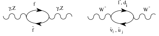
Figure 7: Gauge–boson self-energies (vacuum polarization corrections).

Initial– and final–state photon radiation is by far the most important numerical correction. One has in addition the contributions coming from photon exchange between the fermionic lines. All these QED corrections are to a large extent dependent on the detector and the experimental cuts, because of the infra-red problems associated with massless photons (one needs to define, for instance, the minimun photon energy which can be detected). Therefore, these effects are usually estimated with Monte Carlo programs and subtracted from the data. Notice that in the decay $\mu^{-}\to e^{-}\bar{\nu}_{e}\nu_{\mu}$, the QED corrections are already partly included in the definition of $G_{F}$ thus, one should take care of subtracting those corrections already incorporated in Eq. (18).

More interesting are the so–called oblique corrections, gauge–boson self-energies induced by vacuum polarization diagrams, which are universal (process independent). We have already seen the important role of the photon self-energy. In the case of the $W^{\pm}$ and the $Z$, these corrections are sensitive to heavy particles (such as the top) running along the loop $\!{}^{{\bf?}}$.

In QED, the vacuum polarization contribution of a heavy fermion pair is suppressed by inverse powers of the fermion mass. At low energies ($s<<m_{f}^{2}$), the information on the heavy fermions is then lost. This decoupling of the heavy fields happens in theories like QED and QCD, with only vector couplings and an exact gauge symmetry $\!{}^{{\bf?}}$. The SM involves, however, a broken chiral gauge symmetry. This has the very interesting implication of avoiding the decoupling theorem $\!{}^{{\bf?}}$, offering the possibility to be sensitive to heavy particles which cannot be kinematically accessed.

The $W^{\pm}$ and $Z$ self-energies induced by a heavy top, i.e. $W^{-}\to\bar{t}b\to W^{-}$ and $Z\to\bar{t}t\to Z$, generate contributions which increase quadratically with the top mass $\!{}^{{\bf?}}$. The leading $m_{t}^{2}$ contribution to the $W^{\pm}$ propagator amounts to a $-3\%$ correction to the relation (30) between $G_{F}$ and $M_{W}$.

Owing to an accidental $SU(2)_{C}$ symmetry of the scalar sector (the so–called custodial symmetry), the virtual production of Higgs particles does not generate any $m_{H}^{2}$ dependence at one loop (Veltman screening $\!{}^{{\bf?}}$). The dependence on the Higgs mass is only logarithmic. The numerical size of the correction induced on (30) is $-0.3\%$ ($+1\%$) for $m_{H}=60$ (1000) GeV.

Figure 8: $m_{t}$–dependent corrections to the $Z\bar{b}b$ vertex.

The vertex corrections to the different couplings are non-universal and usually smaller than the oblique contributions. There is one interesting exception, the $Z\bar{b}b$ vertex, which is sensitive to the top quark mass $\!{}^{{\bf?}}$. The $Z\bar{f}f$ vertex gets 1–loop corrections where a virtual $W^{\pm}$ is exchanged between the two fermionic legs. Since, the $W^{\pm}$ coupling changes the fermion flavour, the decays $Z\to\bar{d}d,\bar{s}s,\bar{b}b\$ get contributions with a top quark in the internal fermionic lines. These amplitudes are suppressed by a small quark–mixing factor $|V_{td_{i}}|^{2}$, except for the $Z\to\bar{b}b$ vertex because $|V_{tb}|\approx 1$.

The explicit calculation $\!{}^{{\bf?},{\bf?},{\bf?},{\bf?}}$ shows the presence of hard $m_{t}^{2}$ corrections to the $Z\to\bar{b}b$ vertex. This effect can be easily understood $\!{}^{{\bf?}}$ in non-unitary gauges where the unphysical charged scalar $\phi^{(\pm)}$ is present. The Yukawa couplings of the charged scalar to fermions are proportional to the fermion masses; therefore, the exchange of a virtual $\phi^{(\pm)}$ gives rise to a $m_{t}^{2}$ factor. In the unitary gauge, the charged scalar has been eaten by the $W^{\pm}$ field; thus, the effect comes now from the exchange of a longitudinal $W^{\pm}$, with terms proportional to $q^{\mu}q^{\nu}$ in the propagator that generate fermion masses.

Since the $W^{\pm}$ couples only to left–handed fermions, the induced effect is the same on the vector and axial–vector $Z\bar{b}b$ couplings. It amounts $\!{}^{{\bf?}}$ to a $-1.5\%$ correction of $\Gamma(Z\to\bar{b}b)$.

The non-decoupling present in the $Z\bar{b}b$ vertex is quite different from the one happening in the boson self-energies. The vertex correction does not have any dependence with the Higgs mass. Moreover, while any kind of new heavy particle, coupling to the gauge bosons, would contribute to the $W^{\pm}$ and $Z$ self-energies, possible new–physics contributions to the $Z\bar{b}b$ vertex are much more restricted and, in any case, different. Therefore, an independent experimental test of the two effects is very valuable in order to disentangle possible new–physics contributions from the SM corrections.

The remaining quantum corrections are rather small. Box diagrams with two gauge–boson exchanges give a very small contribution at the $Z$ peak, because they are non resonant (they do not have an on-shell $Z$ propagator). However, the box correction to the decay $\mu^{-}\to e^{-}\bar{\nu}_{e}\nu_{\mu}$ is not negligible. The exchange of a Higgs particle between two fermionic lines is irrelevant, because the amplitude is suppressed by the product of the two fermionic masses.

4.4 Lepton Universality

Table 5: Measured values $\!{}^{{\bf?}}$ of $\Gamma_{l}\equiv\Gamma(Z\to l^{+}l^{-})$ and the leptonic forward–backward asymmetries. The last column shows the combined result (for a massless lepton) assuming lepton universality.

	$e$	$\mu$	$\tau$	$l$
$\Gamma_{l}$   (MeV)	$83.94\pm 0.14$	$83.84\pm 0.20$	$83.68\pm 0.24$	$83.91\pm 0.10$
${\cal A}_{\mbox{\rm\scriptsize FB}}^{0,l}$   (%)	$1.60\pm 0.24$	$1.63\pm 0.14$	$1.92\pm 0.18$	$1.71\pm 0.10$

Table 6: Measured values $\!{}^{{\bf?}}$ of the leptonic polarization asymmetries.

$-{\cal A}_{\mbox{\rm\scriptsize Pol}}^{0,\tau}=-{\cal P}_{\tau}$	$-{4\over 3}{\cal A}^{0,\tau}_{\mbox{\rm\scriptsize FB,Pol}}=-{\cal P}_{e}$	${\cal A}_{\mbox{\rm\scriptsize LR}}^{0}=-{\cal P}_{e}$	$\!\{{4\over 3}{\cal A}_{\mbox{\rm\scriptsize FB}}^{0,l}\}^{1/2}=-P_{l}\!$
$0.1410\pm 0.0064$	$0.1399\pm 0.0073$	$0.1547\pm 0.0032$	$0.1510\pm 0.0044$

Table 7: Effective vector and axial–vector lepton couplings derived from LEP and SLD $\!{}^{{\bf?}}$.

	Without Lepton Universality
	LEP	LEP + SLD
$v_{e}$	$-0.0367\pm 0.0015$	$-0.03844\pm 0.00071$
$v_{\mu}$	$-0.0374\pm 0.0036$	$-0.0358\pm 0.0032$
$v_{\tau}$	$-0.0367\pm 0.0015$	$-0.0365\pm 0.0015$
$a_{e}$	$-0.50123\pm 0.00044$	$-0.50111\pm 0.00043$
$a_{\mu}$	$-0.50087\pm 0.00066$	$-0.50098\pm 0.00065$
$a_{\tau}$	$-0.50102\pm 0.00074$	$-0.50103\pm 0.00074$
$v_{\mu}/v_{e}$	$1.02\pm 0.12$	$\phantom{-}0.932\pm 0.087$
$v_{\tau}/v_{e}$	$0.998\pm 0.060$	$\phantom{-}0.949\pm 0.044$
$a_{\mu}/a_{e}$	$0.9993\pm 0.0017$	$\phantom{-}0.9997\pm 0.0016$
$a_{\tau}/a_{e}$	$0.9996\pm 0.0018$	$\phantom{-}0.9998\pm 0.0018$
	With Lepton Universality
	LEP	LEP + SLD
$v_{l}$	$-0.03681\pm 0.00085$	$-0.03793\pm 0.00058$
$a_{l}$	$-0.50112\pm 0.00032$	$-0.50103\pm 0.00031$
$a_{\nu}=v_{\nu}$	$+0.50125\pm 0.00092$	$+0.50125\pm 0.00092$

Tables 6 and 6 show the present experimental results for the leptonic $Z$ decay widths and asymmetries. The data are in excellent agreement with the SM predictions and confirm the universality of the leptonic neutral couplings. There is however a small $1.9\sigma$ discrepancy between the ${\cal P}_{e}$ values obtained $\!{}^{{\bf?}}$ from ${\cal A}^{0,\tau}_{\mbox{\rm\scriptsize FB,Pol}}$ and ${\cal A}_{\mbox{\rm\scriptsize LR}}^{0}$. The average of the two $\tau$ polarization measurements, ${\cal A}_{\mbox{\rm\scriptsize Pol}}^{0,\tau}$ and ${4\over 3}{\cal A}^{0,\tau}_{\mbox{\rm\scriptsize FB,Pol}}$, results in ${\cal P}_{l}=-0.1406\pm 0.0048$ which disagrees with the ${\cal A}^{0}_{LR}$ measurement at the $2.4\sigma$ level. Assuming lepton universality, the combined result from all leptonic asymmetries gives

$${\cal P}_{l}=-0.1505\pm 0.0023\qquad(\chi^{2}/\mbox{\rm d.o.f.}=6.0/2)\ .$$ (50)

The measurement of ${\cal A}_{\mbox{\rm\scriptsize Pol}}^{0,\tau}$ and ${\cal A}^{0,\tau}_{\mbox{\rm\scriptsize FB,Pol}}$ assumes that the $\tau$ decay proceeds through the SM charged–current interaction. A more general analysis should take into account the fact that the $\tau$ decay width depends on the product $\xi{\cal P}_{\tau}$ where $\xi$ ($=1$ in the SM) is the corresponding Michel parameter in leptonic decays, or the equivalent quantity $\xi_{h}$ ($=h_{\nu_{\tau}}$) in the semileptonic modes. A separate measurement of $\xi$ and ${\cal P}_{\tau}$ has been performed by ALEPH $\!{}^{{\bf?}}$ (${\cal P}_{\tau}=-0.139\pm 0.040$) and L3 $\!{}^{{\bf?}}$ (${\cal P}_{\tau}=-0.154\pm 0.022$), using the correlated distribution of the $\tau^{+}\tau^{-}$ decays.

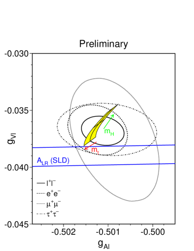
Figure 9: 68% probability contours in the $a_{l}$-$v_{l}$ plane from LEP measurements $\!{}^{{\bf?}}$. The solid contour assumes lepton universality. Also shown is the $1\sigma$ band resulting from the ${\cal A}_{\mbox{\rm\scriptsize LR}}^{0}$ measurement at SLD. The shaded region corresponds to the SM prediction for $m_{t}=175.6\pm 5.5$ GeV and $m_{H}=300^{+700}_{-240}$ GeV. The arrows point in the direction of increasing $m_{t}$ and $m_{H}$ values.

The combined analysis $\!{}^{{\bf?}}$ of all leptonic observables from LEP and SLD (${\cal A}_{\mbox{\rm\scriptsize LR}}^{0}$) results in the effective vector and axial–vector couplings given in Table 7. The corresponding 68% probability contours in the $a_{l}$–$v_{l}$ plane are shown in Figure 9. The measured ratios of the $e$, $\mu$ and $\tau$ couplings provide a test of charged–lepton universality in the neutral–current sector.

The neutrino couplings can be determined from the invisible $Z$–decay width, by assuming three identical neutrino generations with left–handed couplings (i.e., $v_{\nu}=a_{\nu}$), and fixing the sign from neutrino scattering data $\!{}^{{\bf?}}$. The resulting experimental value $\!{}^{{\bf?}}$, given in Table 7, is in perfect agreement with the SM. Alternatively, one can use the SM prediction for $\Gamma_{\mbox{\rm\scriptsize inv}}/\Gamma_{l}$ to get a determination of the number of (light) neutrino flavours $\!{}^{{\bf?}}$:

$$N_{\nu}=2.993\pm 0.011\,.$$ (51)

The universality of the neutrino couplings has been tested with $\nu_{\mu}e$ scattering data, which fixes $\!{}^{{\bf?}}$ the $\nu_{\mu}$ coupling to the $Z$:  $v_{\nu_{\mu}}=a_{\nu_{\mu}}=0.502\pm 0.017$.

Table 8: Determinations $\!{}^{{\bf?}}$ of ${\cal P}_{b}$ and ${\cal P}_{c}$ from LEP data alone (using ${\cal P}_{l}=-0.1461\pm 0.0033$), from SLD data alone, and from LEP + SLD data (using ${\cal P}_{l}=-0.1505\pm 0.0023$) assuming lepton universality.

	LEP	SLD	LEP + SLD
${\cal P}_{b}$	$-0.897\pm 0.030$	$-0.900\pm 0.050$	$-0.877\pm 0.023$
${\cal P}_{c}$	$-0.674\pm 0.046$	$-0.650\pm 0.058$	$-0.653\pm 0.037$

Using the measured value of ${\cal P}_{l}$, one can extract ${\cal P}_{b}$ and ${\cal P}_{c}$ from the forward–backward heavy–flavour asymmetries, measured at LEP. The resulting values are shown in Table 8, together with the direct SLD determinations through ${\cal A}^{0,b/c}_{\mbox{\rm\scriptsize FB,LR}}$, and the combination of LEP and SLD measurements. The LEP results are in excellent agreement with SLD, and in reasonable agreement with the SM predictions (${\cal P}_{b}=-0.935$, ${\cal P}_{c}=-0.668$). However the combined LEP + SLD determination of $|{\cal P}_{b}|$ is about $2.5\sigma$ below the SM. This discrepancy results from the sum of three different effects: the LEP measurement of ${\cal A}^{0,b}_{\mbox{\rm\scriptsize FB}}$ is low ($2.0\sigma$) compared with the SM; the SLD measurement of $|{\cal P}_{b}|$ is also slightly lower ($0.7\sigma$); and ${\cal A}^{0}_{\mbox{\rm\scriptsize LR}}$ is high ($2.4\sigma$) compared to the SM.

Table 9: Comparison of several determinations $\!{}^{{\bf?}}$ of $\sin^{2}{\theta^{\mbox{\rm\scriptsize lept}}_{\mbox{\rm\scriptsize eff}}}$.

	$\sin^{2}{\theta^{\mbox{\rm\scriptsize lept}}_{\mbox{\rm\scriptsize eff}}}$	Average	Cumul. Average	$\chi^{2}/\mbox{\rm dof}$
${\cal A}^{0,l}_{\mbox{\rm\scriptsize FB}}$	$0.23102\pm 0.00056$
${\cal P}_{\tau}$	$0.23228\pm 0.00081$
${\cal P}_{e}$	$0.23243\pm 0.00093$	$0.23162\,(41)$	$0.23162\pm 0.00041$	$2.6/2$
${\cal A}^{0,b}_{\mbox{\rm\scriptsize FB}}$	$0.23236\pm 0.00043$
${\cal A}^{0,c}_{\mbox{\rm\scriptsize FB}}$	$0.23140\pm 0.00111$	$0.23223\,(40)$	$0.23194\pm 0.00029$	$4.3/4$
$\langle Q_{\mbox{\rm\scriptsize FB}}\rangle$	$0.2322\pm 0.0010$	$0.2322\,(10)$	$0.23196\pm 0.00028$	$4.4/5$
${\cal A}^{0}_{\mbox{\rm\scriptsize LR}}$	$0.23055\pm 0.00041$	$0.23055\,(41)$	$0.23152\pm 0.00023$	$12.5/6$

Assuming lepton universality, the measured leptonic asymmetries can be used to obtain the effective electroweak mixing angle in the charged–lepton sector, defined as:

$$\sin^{2}{\theta^{\mbox{\rm\scriptsize lept}}_{\mbox{\rm\scriptsize eff}}}\equiv{1\over 4}\left(1-{v_{l}\over a_{l}}\right)\,.$$ (52)

One can also include the information provided by the hadronic asymmetries, if the hadronic couplings are assumed to be given by the SM; this is justified by the smaller sensitivity of ${\cal P}_{b/c}$ to higher–order corrections. The different determinations $\!{}^{{\bf?}}$ of $\sin^{2}{\theta^{\mbox{\rm\scriptsize lept}}_{\mbox{\rm\scriptsize eff}}}$ and their combination are shown in Table 9.

4.5 SM Electroweak Fit

Including the full SM predictions at the 1–loop level, the $Z$ measurements can be used to obtain information on the SM parameters. The high accuracy of the present data provides compelling evidence for the pure weak quantum corrections, beyond the main QED and QCD corrections discussed in Section 4.2. The measurements are sufficiently precise to require the presence of quantum corrections associated with the virtual exchange of top quarks, gauge bosons and Higgses.

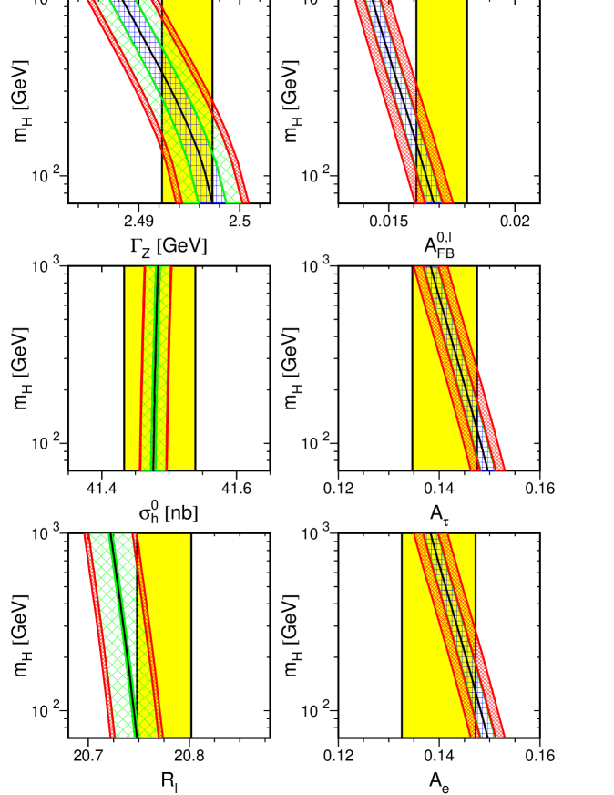
Figure 10: Comparison $\!{}^{{\bf?}}$ of LEP measurements with the SM predictions as a function of $m_{H}$.

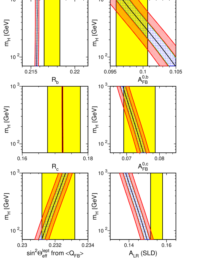
Figure 11: Comparison $\!{}^{{\bf?}}$ of LEP measurements with the SM predictions as a function of $m_{H}$. Also shown is the SLD measurement of ${\cal A}^{0}_{\mbox{\rm\scriptsize LR}}$.

Figures 10 and 11, taken from Ref. 37, compare different LEP measurements with the corresponding SM predictions as a function of the Higgs mass; also shown is the SLD measurement of ${\cal A}^{0}_{\mbox{\rm\scriptsize LR}}$. The cross-hatch pattern parallel to the axes indicates the variation of the SM prediction with $m_{t}=175.6\pm 5.5$ GeV; the coarse diagonal cross-hatch pattern corresponds to a variation of the strong coupling in the range $\alpha_{s}(M_{Z}^{2})=0.118\pm 0.003$; and the dense diagonal cross-hatching to the variation of $\alpha^{-1}(M_{Z}^{2})=128.896\pm 0.090$. The experimental errors on the measured parameters are indicated as vertical bands. For the comparison of $R_{b}$ with the SM the value of $R_{c}$ has been fixed to the SM prediction. The overall agreement is good. As can be seen, the asymmetries are the most sensitive observables to $m_{H}$.

Notice that the uncertainty on $\alpha(M_{Z}^{2})^{-1}$ introduces a severe limitation on the accuracy of the SM predictions. To improve the present determination of $\alpha(M_{Z}^{2})^{-1}$ one needs to perform a good measurement of $\sigma(e^{+}e^{-}\to\mbox{\rm hadrons})$, as a function of the centre–of–mass energy, in the whole kinematical range spanned by DA$\Phi$NE, a tau–charm factory and the B factories. This would result in a much stronger constraint on the Higgs mass.

Table 10: Results from the global electroweak fits $\!{}^{{\bf?}}$ to LEP data alone, to all data except the direct measurements of $m_{t}$ and $M_{W}$ at Tevatron and LEP2, and to all data.

	LEP only	All data except	All data
	($M_{W}$ included)	$m_{t}$ and $M_{W}$
$m_{t}$    (GeV)	$158{\,}^{+14}_{-11}$	$157{\,}^{+10}_{-9}$	$173.1\pm 5.4$
$m_{H}$    (GeV)	$83{\,}^{+168}_{-49}$	$41{\,}^{+64}_{-21}$	$115{\,}^{+116}_{-66}$
$\log{(m_{H})}$	$1.92{\,}^{+0.48}_{-0.39}$	$1.62{\,}^{+0.41}_{-0.31}$	$2.06{\,}^{+0.30}_{-0.37}$
$\alpha_{s}(M_{Z}^{2})$	$0.121\pm 0.003$	$0.120\pm 0.003$	$0.120\pm 0.003$
$\chi^{2}/\mbox{\rm d.o.f.}$	$8/9$	$14/12$	$17/15$
$\sin^{2}{\theta^{\mbox{\rm\scriptsize lept}}_{\mbox{\rm\scriptsize eff}}}$	$0.23188\pm 0.00026$	$0.23153\pm 0.00023$	$0.23152\pm 0.00022$
$1-M_{W}^{2}/M_{Z}^{2}$	$0.2246\pm 0.0008$	$0.2240\pm 0.0008$	$0.2231\pm 0.0006$
$M_{W}$    (GeV)	$80.298\pm 0.043$	$80.329\pm 0.041$	$80.375\pm 0.030$

Table 10 shows the constraints obtained on $m_{t}$, $m_{H}$ and $\alpha_{s}(M_{Z}^{2})$, from a global fit to the electroweak data $\!{}^{{\bf?}}$. As the sensitivity to the Higgs mass is logarithmic, the fitted values of $\log{(m_{H})}$ are also quoted. The bottom part of the table lists derived results for $\sin^{2}{\theta^{\mbox{\rm\scriptsize lept}}_{\mbox{\rm\scriptsize eff}}}$, $1-M_{W}^{2}/M_{Z}^{2}$ and $M_{W}$.

Three different fits are shown. The first one uses only LEP data, including the LEP2 determination of $M_{W}$. The fitted value of the top mass is in good agreement with the Tevatron measurement $\!{}^{{\bf?}}$, $m_{t}=175.6\pm 5.5$ GeV, although slightly lower. The data seems to prefer also a light Higgs. There is a large correlation (0.76) between the fitted values of $m_{t}$ and $m_{H}$; the correlation would be much larger if the $R_{b}$ measurement was not used ($R_{b}$ is insensitive to $m_{H}$). The extracted value of the strong coupling agrees very well with the world average value $\!{}^{{\bf?}}$ $\alpha_{s}(M_{Z}^{2})=0.118\pm 0.003$.

The second fit includes all electroweak data except the direct measurements of $m_{t}$ and $M_{W}$, performed at Tevatron and LEP2. The fitted values for these two masses agree well with the direct determinations. The indirect measurements clearly prefer low $m_{t}$ and low $m_{H}$.

Table 11: Summary $\!{}^{{\bf?}}$ of measurements included in the global analysis of electroweak data. The third and fourth column show the fitted values obtained within the SM and the associated pulls (difference between measurement and fit in units of the measurement error).

	Measurement	SM fit	Pull
$M_{Z}$    (GeV)	$91.1867\pm 0.0020$	$91.1866$	$0.0$
$\Gamma_{Z}$    (GeV)	$2.4948\pm 0.0025$	$2.4966$	$-0.7$
$\sigma^{0}_{\mbox{\rm\scriptsize had}}$    (nb)	$41.486\pm 0.053$	$41.467$	$0.4$
$R_{l}$	$20.775\pm 0.027$	$20.756$	$0.7$
${\cal A}^{0,l}_{\mbox{\rm\scriptsize FB}}$	$0.0171\pm 0.0010$	$0.0162$	$0.9$
${\cal P}_{\tau}$	$-0.1411\pm 0.0064$	$-0.1470$	$0.9$
${4\over 3}{\cal A}^{0,\tau}_{\mbox{\rm\scriptsize FB,Pol}}$	$-0.1399\pm 0.0073$	$-0.1470$	$1.0$
$R_{b}$	$0.2170\pm 0.0009$	$0.2158$	$1.3$
$R_{c}$	$0.1734\pm 0.0048$	$0.1723$	$0.2$
${\cal A}^{0,b}_{\mbox{\rm\scriptsize FB}}$	$0.0984\pm 0.0024$	$0.1031$	$-2.0$
${\cal A}^{0,c}_{\mbox{\rm\scriptsize FB}}$	$0.0741\pm 0.0048$	$0.0736$	$0.1$
${\cal P}_{b}$	$-0.900\pm 0.050$	$-0.935$	$0.7$
${\cal P}_{c}$	$-0.650\pm 0.058$	$-0.668$	$0.3$
$\sin^{2}{\theta^{\mbox{\rm\scriptsize lept}}_{\mbox{\rm\scriptsize eff}}}$    ($\langle Q_{\mbox{\rm\scriptsize FB}}\rangle$)	$0.2322\pm 0.0010$	$0.23152$	$0.7$
$\sin^{2}{\theta^{\mbox{\rm\scriptsize lept}}_{\mbox{\rm\scriptsize eff}}}$    (${\cal A}^{0}_{\mbox{\rm\scriptsize LR}}$)	$0.23055\pm 0.00041$	$0.23152$	$-2.4$
$M_{W}$    (GeV)	$80.43\pm 0.08$	$80.375$	$0.7$
$m_{t}$    (GeV)	$175.6\pm 5.5$	$173.1$	$0.4$
$1-M_{W}^{2}/M_{Z}^{2}$    ($\nu N$)	$0.2254\pm 0.0037$	$0.2231$	$0.6$

The best constraints on $m_{H}$ are obtained in the last fit, which includes all available data. Taking into account additional theoretical uncertainties (not included in Table 10) due to the missing higher–order corrections, the global fit results in the upper bound $\!{}^{{\bf?}}$:

$$m_{H}<420\;\mbox{\rm GeV}\qquad(95\%\,\mbox{\rm CL})\,.$$ (53)

The quality of the global electroweak fit can better appreciated in Table 11, where the input measurements are compared with the resulting SM values. The pulls indicate the differences between the measurements and the corresponding fit values in units of the experimental errors. The global agreement is quite good. The distribution of the pulls, with a few $2\sigma$ deviations, is more or less what one should expect statistically. As already mentioned before, the largest discrepancies occur in ${\cal A}^{0}_{\mbox{\rm\scriptsize LR}}$ and ${\cal A}^{0,b}_{\mbox{\rm\scriptsize FB}}$.

5 Summary

The SM provides a beautiful theoretical framework which is able to accommodate all our present knowledge on electroweak interactions. It is able to explain any single experimental fact and, in some cases, it has successfully passed very precise tests at the 0.1% to 1% level. However, there are still pieces of the SM Lagrangian which so far have not been experimentally analyzed in any precise way.

The gauge self-couplings are presently being investigated at LEP2, through the study of the $e^{+}e^{-}\to W^{+}W^{-}$ production cross-section. The $V-A$ ($\nu_{e}$-exchange in the $t$ channel) contribution generates an unphysical growing of the cross-section with the centre-of-mass energy, which is compensated through a delicate gauge cancellation with the $e^{+}e^{-}\to\gamma,Z\to W^{+}W^{-}$ amplitudes. The recent LEP2 measurements of $\sigma(e^{+}e^{-}\to W^{+}W^{-})$ at 172 GeV, in good agreement with the SM, have provided already convincing evidence $\!{}^{{\bf?},{\bf?}}$ for the contribution coming from the $ZWW$ vertex. With more statistics, it will be possible to make a detailed investigation of the gauge–boson self-interactions.

The study of this process will also provide a more accurate measurement of $M_{W}$, allowing to improve the precision of the neutral–current analyses. The present LEP2 determination, $M_{W}=80.48\pm 0.14$ GeV, is already competitive with the value $M_{W}=80.41\pm 0.09$ GeV obtained in $p\bar{p}$ colliders, but its error is still too large compared with the 41 MeV sensitivity achieved with the indirect SM fit of electroweak data. To achieve this sort of accuracy is one of the main goals of LEP2.

The Higgs particle is the main missing block of the SM framework. The data provide a clear confirmation of the assumed pattern of spontaneous symmetry breaking, but do not prove the minimal Higgs mechanism embedded in the SM. At present, a relatively light Higgs seems to be preferred by the indirect precision tests. LEP2 first and later LHC will try to find out whether such scalar field exists.

In spite of its enormous phenomenological success, the SM leaves too many unanswered questions to be considered as a complete description of the fundamental forces. We do not understand yet why fermions are replicated in three (and only three) nearly identical copies? Why the pattern of masses and mixings is what it is? Are the masses the only difference among the three families? What is the origin of the SM flavour structure? Which dynamics is responsible for the observed CP violation?

Clearly, we need more experiments in order to learn what kind of physics exists beyond the present SM frontiers. We have, fortunately, a very promising and exciting future ahead of us.

References

References

- [1] A. Pich, The Standard Model of Electroweak Interactions, Proc. XXII International Winter Meeting on Fundamental Physics: The Standard Model and Beyond (Jaca, 7–11 February 1994), eds. J.A. Villar and A. Morales (Editions Frontières, Gif-sur-Yvette, 1995), p. 1 [hep-ph/9412274].
- [2] A. Pich, Quantum Chromodynamics, Proc. 1994 European School of High Energy Physics (Sorrento, 29 August – 11 September 1994), eds. N. Ellis and M.B. Gavela, Report CERN 95-04 (Geneva, 1995), p. 157 [hep-ph/9505231].
- [3] A. Pich, Flavourdynamics, Proc. XXIII International Winter Meeting on Fundamental Physics: The Top Quark, Heavy Flavour Physics and Symmetry Breaking (Comillas, 22–26 May 1995), eds. T. Rodrigo and A. Ruiz (World Scientific, Singapore, 1996), p. 1 [hep-ph/9601202].
- [4] A. Pich, Weak Decays, Quark Mixing and CP Violation: Theory Overview, Proc. XVI International Workshop on Weak Interactions and Neutrinos (Capri, 1997), eds. G. Fiorillo et al, Nucl. Phys. B (Proc. Suppl.), in press [hep-ph/9709441].
- [5] W.J. Marciano, Nucl. Phys. B (Proc. Suppl.) 40 (1995) 3.
- [6] H.-U. Martyn, Test of QED by High Energy Electron–Positron Collisions, in Ref. 7, p. 92.
- [7] T. Kinoshita (editor), Quantum Electrodynamics, Advanced Series on Directions in High Energy Physics, Vol. 7 (World Scientific, Singapore, 1990).
- [8] T. Kinoshita, Rep. Prog. Phys. 59 (1996) 1459.
- [9] A. Czarnecki, B. Krause and W.J. Marciano, Phys. Rev. Lett. 76 (1996) 3267; Phys. Rev. D52 (1995) 2619.
- [10] S. Peris, M. Perrotet and E. de Rafael, Phys. Lett. B355 (1995) 523.
- [11] T.V. Kukhto et al, Nucl. Phys. B371 (1992) 567.
- [12] E. de Rafael, Phys. Lett. B322 (1994) 239.
- [13] M. Hayakawa and T. Kinoshita, hep-ph/9708227.
- [14] M. Hayakawa, T. Kinoshita and A.I. Sanda, Phys. Rev. D54 (1996) 3137.
- [15] T. Kinoshita and A.I. Sanda, Phys. Rev. Lett. 75 (1995) 790.
- [16] J. Bijnens, E. Pallante and J. Prades, Nucl. Phys. B474 (1996) 379; Phys. Rev. Lett. 75 (1995) 1447, 3781.
- [17] B. Krause, Phys. Lett. B390 (1997) 392.
- [18] R. Alemany, M. Davier and A. Höcker, hep-ph/9703220.
- [19] Particle Data Group, Review of Particle Properties, Phys. Rev. D54 (1996) 1; and 1997 off-year partial update for the 1998 edition [URL:http://pdg.lbl.gov/].
- [20] The Second DANE Physics Handbook, eds. L. Maiani, G. Panchieri and N. Paver (Frascati, 1995).
- [21] B.L. Roberts et al (BNL-E821), Status of the New Muon Experiment, Proc. 28th International Conference on High Energy Physics (Warsaw, 1996), eds. Z. Ajduk and A.K. Wroblewski (World Scientific, Singapore, 1997), p. 1035.
- [22] D.J. Silverman and G.L. Shaw, Phys. Rev. D27 (1983) 1196.
- [23] L. Taylor, Nucl. Phys. B (Proc. Suppl.) 55C (1997) 285.
- [24] R. Escribano and E. Masso, Phys. Lett. B301 (1993) 419; Nucl. Phys. B429 (1994) 19; Phys. Lett. B395 (1997) 369.
- [25] J.S. Schwinger, Phys. Rev. 73 (1948) 416.
- [26] S. Narison, J. Phys. G: Nucl. Phys. 4 (1978) 1849.
- [27] M.A. Samuel, G. Li and R. Mendel, Phys. Rev. Lett. 67 (1991) 668.
- [28] T. Kinoshita and A. Sirlin, Phys. Rev. 113 (1959) 1652.
- [29] W.J. Marciano and A. Sirlin, Phys. Rev. Lett. 61 (1988) 1815.
- [30] R. Barate et al (ALEPH), CERN-PPE/97-090 [hep-ex/9710026].
- [31] A. Pich, Nucl. Phys. B (Proc. Suppl.) 55C (1997) 3.
- [32] L. Passalacqua, Nucl. Phys. B (Proc. Suppl.) 55C (1997) 435.
- [33] W.J. Marciano and A. Sirlin, Phys. Rev. Lett. 71 (1993) 3629.
- [34] R. Decker and M. Finkemeier, Nucl. Phys. B438 (1995) 17; Nucl. Phys. B (Proc. Suppl.) 40 (1995) 453.
- [35] D.I. Britton et al, Phys. Rev. Lett. 68 (1992) 3000.
- [36] G. Czapek et al, Phys. Rev. Lett. 70 (1993) 17.
- [37] The LEP Collaborations ALEPH, DELPHI, L3, OPAL, the LEP Electroweak Working Group and the SLD Heavy Flavour Group, A Combination of Preliminary Electroweak Measurements and Constraints on the Standard Model, CERN preprint LEPEWWG/97-02 (18 August 1997).
- [38] L. Michel, Proc. Phys. Soc. A63 (1950) 514; 1371.
- [39] C. Bouchiat and L. Michel, Phys. Rev. 106 (1957) 170.
- [40] T. Kinoshita and A. Sirlin, Phys. Rev. 107 (1957) 593; 108 (1957) 844.
- [41] F. Scheck, Leptons, Hadrons and Nuclei (North-Holland, Amsterdam, 1983); Phys. Rep. 44 (1978) 187.
- [42] W. Fetscher, H.-J. Gerber and K.F. Johnson, Phys. Lett. B173 (1986) 102.
- [43] W. Fetscher and H.-J. Gerber, Precision Measurements in Muon and Tau Decays, in Precision Tests of the Standard Electroweak Model, ed. P. Langacker, Advanced Series on Directions in High Energy Physics – Vol. 14 (World Scientific, Singapore, 1995), p. 657.
- [44] A. Pich and J.P. Silva, Phys. Rev. D52 (1995) 4006.
- [45] D. Guill, in Proc. XVI International Workshop on Weak Interactions and Neutrinos (Capri, 1997), eds. G. Fiorillo et al, Nucl. Phys. B (Proc. Suppl.), in press.
- [46] J.P. Alexander et al (CLEO), CLNS 97/1480 [hep-ex/9705009].
- [47] W. Lohmann and J. Raab, Charged Current Couplings in Decay, DESY 95-188.
- [48] R. Alemany et al, Nucl. Phys. B379 (1992) 3.
- [49] S. Eidelmann and F. Jegerlehner, Z. Phys. C67 (1995) 585.
- [50] M. Veltman, Nucl. Phys. B123 (1977) 89.
- [51] T. Appelquist and J. Carazzone, Phys. Rev. D11 (1975) 2856.
- [52] J. Bernabéu, A. Pich and A. Santamaría, Phys. Lett. B200 (1988) 569; Nucl. Phys. B363 (1991) 326.
- [53] A.A. Akhundov, D. Yu. Bardin and T. Riemann, Nucl. Phys. B276 (1986) 1.
- [54] W. Beenakker and W. Hollik, Z. Phys. C40 (1988) 141.
- [55] B.W. Lynn and R.G. Stuart, Phys. Lett. B252 (1990) 676.
- [56] D. Buskulic et al (ALEPH), Phys. Lett. B321 (1994) 168.
- [57] M. Acciarri et al (L3), Phys. Lett. B377 (1996) 313.
- [58] J. Bernabéu, A. Pich and N. Rius, Phys. Lett. B257 (1991) 219.
- [59] R. Barate et al (ALEPH, Phys. Lett. B405 (1997) 191.
- [60] P. Abreu et al (DELPHI), CERN-PPE/97-34.
- [61] P. Vilain et al (CHARM II), Phys. Lett. B335 (1994) 246.
- [62] P. Vilain et al (CHARM II), Phys. Lett. B320 (1994) 203.
- [63] R. Miquel, Physics at LEP2, these proceedings.