Non-perturbative renormalization of QCD¹

Abstract

In these lectures, we discuss different types of renormalization problems in QCD and their non-perturbative solution in the framework of the lattice formulation. In particular the recursive finite size methods to compute the scale-dependence of renormalized quantities is explained. An important ingredient in the practical applications is the Schrödinger functional. It is introduced and its renormalization properties are discussed.
Concerning applications, the computation of the running coupling and the running quark mass are covered in detail and it is shown how the $\Lambda$-parameter and renormalization group invariant quark mass can be obtained. Further topics are the renormalization of isovector currents and non-perturbative Symanzik improvement.
Contents

• Introduction
  Basic renormalization: hadron spectrum; Finite renormalization: (semi-)leptonic decays; Scale dependent renormalization; Irrelevant operators

• The problem of scale dependent renormalization
  The extraction of $\alpha$ from experiments; Reaching large scales in lattice QCD

• The Schrödinger functional
  Definition; Quantum mechanical interpretation; Background field; Perturbative expansion; General renormalization properties; Renormalized coupling; Quarks; Renormalized mass; Lattice formulation

• The computation of $\alpha(q)$
  The step scaling function; Lattice spacing effects in perturbation theory; The continuum limit – universality; The running of the coupling; The low energy scale; Matching at finite energy; The $\Lambda$ parameter of quenched QCD; The use of bare couplings

• Renormalization group invariant quark mass

• Chiral symmetry, normalization of currents and ${\rm O}(a)$-improvement
  Chiral Ward identities; ${\rm O}(a)$-improvement; Normalization of isovector currents

• Summary, Conclusions

DESY 97-207

1 Introduction

The topic of these lectures is the computation of properties of particles that are bound by the strong interaction or more generally interact strongly. The strong interactions are theoretically described by Quantum Chromo Dynamics (QCD), a local quantum field theory.

Starting from the Lagrangian of a field theory, predictions for cross sections and other observables are usually made by applying renormalized perturbation theory, the expansion in terms of the (running) couplings of the theory. While this expansion is well controlled as far as electroweak interactions are concerned, its application in QCD is limited to high energy processes where the QCD coupling, $\alpha$, is sufficiently small. In general – and in particular for the calculation of bound state properties – a non-perturbative solution of the theory is required.

The only method that is known to address this problem is the numerical simulation of the Euclidean path integral of QCD on a space-time lattice. By “solution of the theory” we here mean that one poses a well defined question like “what is the value of the $\pi$ decay constant”, and obtains the answer (within a certain precision) through a series of Monte Carlo (MC) simulations. This then allows to test the agreement of theory and experiment on the one hand and helps in the determination of Standard Model parameters from experiments on the other hand.

Quantum field theories are defined by first formulating them in a regularization with an ultraviolet cutoff $\Lambda_{\rm cut}$ and then considering the limit $\Lambda_{\rm cut}\to\infty$. In the lattice formulation ([Wilson]), the cutoff is given by the inverse of the lattice spacing $a$; we have to consider the continuum limit $a\to 0$. At a finite value of $a$, the theory is defined in terms of the bare coupling constant, bare masses and bare fields. Before making predictions for experimental observables (or more generally for observables that have a well defined continuum limit) the coupling, masses and fields have to be renormalized. This is the subject of my lectures.

Renormalization is an ultraviolet phenomenon with relevant momentum scales of order $a^{-1}$. Since $\alpha$ becomes weak in the ultraviolet, one expects to be able to perform renormalizations perturbatively, i.e. computed in a power series in $\alpha$ as one approaches the continuum limit $a\to 0$. However, one has to take care about the following point. In order to keep the numerical effort of a simulation tractable, the number of degrees of freedom in the simulation may not be excessively large. This means that the lattice spacing $a$ can not be taken very much smaller than the relevant physical length scales of the observable that is considered. Consequently the momentum scale $a^{-1}$ that is relevant for the renormalization is not always large enough to justify the truncation of the perturbative series. In order to obtain a truly non-perturbative answer, the renormalizations have to be performed non-perturbatively.

Depending on the observable, the necessary renormalizations are of different nature. I will use this introduction to point out the different types and in particular explain the problem that occurs in a non-perturbative treatment of renormalization.

1.1 Basic renormalization: hadron spectrum

At this school, the calculation of the hadron spectrum is covered in detail in the lectures of Don Weingarten ([Don]). I mention it anyway because I want to make the conceptual point that it can be considered as a non-perturbative renormalization. I refer the reader to Weingarten’s lectures both for details in such calculations and for an introduction to the basics of lattice QCD.

The calculation starts by choosing certain values for the bare coupling, $g_{0}$, and the bare masses of the quarks in units of the lattice spacing, $am_{0}^{f}$. The flavor index $f$ assumes values $f={\rm u,d,s,c,b}$ for the up, down, charm and bottom quarks that are sufficient to describe hadrons of up to a few ${\rm GeV}$ masses. We neglect isospin breaking and take the light quarks to be degenerate, $m_{0}^{\rm u}=m_{0}^{\rm d}=m_{0}^{\rm l}$.

Next, from MC simulations of suitable correlation functions, one computes masses of five different hadrons $H$, e.g. $H={\rm p},\pi,{\rm K,D,B}$ for the proton, the pion and the K-,D- and B-mesons,

$$am_{H}=am_{H}(g_{0},am_{0}^{\rm l},am_{0}^{\rm s},am_{0}^{\rm c},am_{0}^{\rm b})\enspace.$$ (1)

The theory is renormalized by first setting $m_{\rm p}=m_{\rm p}^{\rm exp}$, where $m_{\rm p}^{\rm exp}$ is the experimental value of the proton mass. This determines the lattice spacing via

$$a=(am_{\rm p})/{m_{\rm p}^{\rm exp}}\enspace.$$ (2)

Next one must choose the parameters $am_{0}^{f}$ such that (1) is indeed satisfied with the experimental values of the meson masses. Equivalently, one may say that at a given value of $g_{0}$ one fixes the bare quark masses from the condition

$$(am_{H})/(am_{\rm p})=m_{H}^{\rm exp}/m_{\rm p}^{\rm exp}\,,\quad H=\pi,{\rm K,D,B}\enspace.$$ (3)

and the bare coupling $g_{0}$ then determines the value of the lattice spacing through (2).

After this renormalization, namely the elimination of the bare parameters in favor of physical observables, the theory is completely defined and predictions may be made. E.g. the mass of the $\Delta$-resonance can be determined,

$$m_{\Delta}=a^{-1}[am_{\Delta}][1+{\rm O}(a)]\enspace.$$ (4)

For the rest of this section, I assume that the bare parameters have been eliminated and consider the additional renormalizations of more complicated observables.

Note.

Renormalization as described here is done without any reference to perturbation theory. One could in principle use the perturbative formula for $(a\Lambda)(g_{0})$ for the renormalization of the bare coupling, where $\Lambda$ denotes the $\Lambda$-parameter of the theory. Proceeding in this way, one obtains a further prediction namely $m_{\rm p}/\Lambda$ but at the price of introducing ${\rm O}(g_{0}^{2})$ errors in the prediction of the observables. As mentioned before, such errors decrease very slowly as one performs the continuum limit. A better method to compute the $\Lambda$-parameter will be discussed later.

1.2 Finite renormalization: (semi-)leptonic decays

Semileptonic weak decays of hadrons such as ${\rm K}\to\pi\,\,e\,\,\bar{\nu}$ are mediated by electroweak vector bosons. These couple to quarks through linear combinations of vector and axial vector flavor currents. Treating the electroweak interactions at lowest order, the decay rates are given in terms of QCD matrix elements of these currents. For simplicity we consider only two flavors; an application is then the computation of the pion decay constant describing the leptonic decay $\pi\to e\,\,\bar{\nu}$. The currents are

$$A_{\mu}^{a}(x) = \overline{\psi}(x)\gamma_{\mu}\gamma_{5}\hbox{$1\over 2$}\tau^{a}\psi(x)\enspace,$$

$$V_{\mu}^{a}(x) = \overline{\psi}(x)\gamma_{\mu}\hbox{$1\over 2$}\tau^{a}\psi(x)\enspace,$$ (5)

where $\tau^{a}$ denote the Pauli matrices which act on the flavor indices of the quark fields. A priori the bare currents (5) need renormalization. However, in the limit of vanishing quark masses the (formal continuum) QCD Lagrangian is invariant under SU$(2)_{\rm V}\times$ SU$(2)_{\rm A}$ flavor symmetry transformations. This leads to nonlinear relations between the currents called current algebra, from which one concludes that no renormalization is necessary (cf. Sect. 6).

In the regularized theory SU$(2)_{\rm V}\times$ SU$(2)_{\rm A}$ is not an exact symmetry but is violated by terms of order $a$. As a consequence there is a finite renormalization ([Za1, Za2, Za3, Za4, Za5])

$$(A_{{\rm R}})_{\mu}^{a} = Z_{\rm A}A_{\mu}^{a}\enspace,$$

$$(V_{{\rm R}})_{\mu}^{a} = Z_{\rm V}V_{\mu}^{a}\enspace,$$ (6)

with renormalization constants $Z_{\rm A},Z_{\rm V}$ that do not contain any logarithmic (in $a$) or power law divergences and do not depend on any physical scale. Rather they are approximated by

$$Z_{\rm A}=1+Z_{\rm A}^{(1)}g_{0}^{2}+\ldots\enspace,$$

$$Z_{\rm V}=1+Z_{\rm V}^{(1)}g_{0}^{2}+\ldots\enspace,$$ (7)

for small $g_{0}$.

On the non-perturbative level these renormalizations can be fixed by current algebra relations ([Boch, MaMa, paper4]) as will be explained in section 6.

1.3 Scale dependent renormalization

1.3.1 a) Short distance parameters of QCD.

As we take the relevant length scales in correlation functions to be small or take the energy scale in scattering processes to be high, QCD becomes a theory of weakly coupled quarks and gluons. The strength of the interaction may be measured for instance by the ratio of the production rate of three jets to the rate for two jets in high energy $e^{+}~{}e^{-}$ collisions,

$$\alpha(q) \propto {\sigma(e^{+}~{}e^{-}\to q~{}\bar{q}~{}g)\over\sigma(e^{+}~{}e^{-}\to q~{}\bar{q})}\,,\quad q^{2}=(p_{e^{-}}+p_{e^{+}})^{2}\gg 10{\rm GeV}^{2}\enspace.$$ (8)

We observe the following points.

• The perturbative renormalization group tells us that $\alpha(q)$ decreases logarithmically with growing energy $q$. In other words the renormalization from the bare coupling to a renormalized one is logarithmically scale dependent.

• Different definitions of $\alpha$ are possible; but with increasing energy, $\alpha$ depends less and less on the definition (or the process).

• In the same way, running quark masses $\kern 1.0pt\overline{\kern-1.0ptm\kern-1.0pt}\kern 1.0pt$ acquire a precise meaning at high energies.

• Using a suitable definition (scheme), the $q$-dependence of $\alpha$ and $\kern 1.0pt\overline{\kern-1.0ptm\kern-1.0pt}\kern 1.0pt$ can be determined non-perturbatively and at high energies the short distance parameters $\alpha$ and $\kern 1.0pt\overline{\kern-1.0ptm\kern-1.0pt}\kern 1.0pt$ can be converted to any other scheme using perturbation theory in $\alpha$.

Explaining these points in detail is the main objective of my lectures. For now we proceed to give a second example of scale dependent renormalization.

1.3.2 b) Weak hadronic matrix elements of 4-quark operators.

Another example of scale dependent renormalization is the 4-fermion operator, $O^{\Delta_{s}=2}$, which changes strangeness by two units. It originates from weak interactions after integrating out the fields that have high masses. It describes the famous mixing in the neutral Kaon system through the matrix element

$$\langle\overline{\rm K}^{0}|O^{\Delta_{s}=2}(\mu)|{\rm K}^{0}\rangle\enspace.$$

Here the operator renormalized at energy scale $\mu$ is given by

$$O^{\Delta_{s}=2}(\mu) = Z^{\Delta_{s}=2}(\mu a,g_{0})\left\{{\overline{\psi}_{s}}\gamma_{\mu}^{\rm L}\psi_{d}\,{\overline{\psi}_{s}}\gamma_{\mu}^{\rm L}\psi_{d}+\sum_{j={\rm S,P,V,A,T}}z_{j}{\overline{\psi}_{s}}\Gamma_{j}\psi_{d}\,{\overline{\psi}_{s}}\Gamma_{j}\psi_{d}\right\}\enspace,$$ (9)

$$\gamma_{\mu}^{\rm L}=\hbox{$1\over 2$}\gamma_{\mu}(1-\gamma_{5})\enspace,$$

$$\Gamma_{\rm S}=1,\,\Gamma_{\rm P}=\gamma_{5},\,\ldots,\Gamma_{\rm T}=\sigma_{\mu\nu}\enspace,$$

$$z_{j}={\rm O}(g_{0}^{2}),\quad z_{\rm V}=-z_{\rm A}$$

where I have indicated the flavor index of the quarks explicitly. A mixing of the leading bare operator, ${\overline{\psi}_{s}}\gamma_{\mu}^{\rm L}\psi_{d}\,{\overline{\psi}_{s}}\gamma_{\mu}^{\rm L}\psi_{d}$, with operators of different chirality is again possible since the lattice theory does not have an exact chiral symmetry for finite values of the lattice spacing. The mixing coefficients $z_{j}$ may be fixed non-perturbatively by current algebra ([Wardid_jap]). Afterwards, the overall scale dependent renormalization has to be treated in the same way as the renormalization of the coupling.

1.4 Irrelevant operators

A last category of renormalization is associated with the removal of lattice discretization errors such as the ${\rm O}(a)$-term in (4). Following Symanzik’s improvement program, this can be achieved order by order in the lattice spacing by adding irrelevant operators, i.e. operators of dimension larger than four, to the lattice Lagrangian ([Symanzik]). The coefficients of these operators are easily determined at tree level of perturbation theory, but in general they need to be renormalized.

In this subject significant progress has been made recently as reviewed by [Lepage96, Sommer97]. In particular the latter reference is concerned with non-perturbative Symanzik improvement and uses a notation consistent with the one of these lectures. It will become evident in later sections that improvement is very important for the progress in lattice QCD.

Note also the alternative approach of removing lattice artifacts order by order in the coupling constant but non-perturbatively in the lattice spacing $a$ as recently reviewed by [Nieder].

2 The problem of scale dependent renormalization

Let us investigate the extraction of short distance parameters (Section 1.3a) in more detail. First we analyze the conventional way of obtaining $\alpha$ from experiments. Then we explain how one can compute $\alpha$ at large energy scales using lattice QCD.

2.1 The extraction of $\alpha$ from experiments

One considers experimental observables $O_{i}$ depending on an overall energy scale $q$ and possibly some additional kinematical variables denoted by $y$. The observables can be computed in a perturbative series which is usually written in terms of the $\overline{\rm MS}$ coupling $\alpha_{{\rm\overline{MS\kern-0.35002pt}\kern 0.35002pt}}$,

$$O_{i}(q,y) = \alpha_{{\rm\overline{MS\kern-0.35002pt}\kern 0.35002pt}}(q)+A_{i}(y)\alpha_{{\rm\overline{MS\kern-0.35002pt}\kern 0.35002pt}}^{2}(q)+\ldots\enspace.$$ (10)

For example $O_{i}$ may be constructed from jet cross sections and $y$ may be related to the details of the definition of a jet.

The renormalization group describes the energy dependence of $\alpha$ in a general scheme ($\alpha\equiv\bar{g}^{2}/(4\pi)$),

$$q{\partial\bar{g}\over\partial q} = \beta(\bar{g})\enspace,$$ (11)

where the $\beta$-function has an asymptotic expansion

$$\beta(\bar{g}) \buildrel{\bar{g}}\rightarrow 0\over{\sim} -{\bar{g}}^{3}\left\{b_{0}+{\bar{g}}^{2}b_{1}+\ldots\right\}\enspace,$$ (12)

$$b_{0}=\hbox{$1\over(4\pi)^{2}$}\bigl{(}11-\hbox{$2\over 3$}N_{\rm f}\bigr{)}\enspace,$$

$$b_{1}=\hbox{$1\over(4\pi)^{4}$}\bigl{(}102-\hbox{$38\over 3$}N_{\rm f}\bigr{)}\enspace,$$

with higher order coefficients $b_{i},\,i>1$ that depend on the scheme. (12) entails the aforementioned property of asymptotic freedom: at energies that are high enough for (12) to be applicable and for a number of quark flavors, $N_{\rm f}$, that is not too large, $\alpha$ decreases with increasing energy as indicated in Fig. 1. The asymptotic solution of (11) is given by

$$\bar{g}^{2} \buildrel{q}\rightarrow\infty\over{\sim} {1\over b_{0}\ln(q^{2}/\Lambda^{2})}-{b_{1}\ln[\ln(q^{2}/\Lambda^{2})]\over b_{0}^{3}[\ln(q^{2}/\Lambda^{2})]^{2}}+{\rm O}\left({\{\ln[\ln(q^{2}/\Lambda^{2})]\}^{2}\over[\ln(q^{2}/\Lambda^{2})]^{3}}\right)$$ (13)

with $\Lambda$ an integration constant which is different in each scheme.

Figure 1: Running of $\alpha$ in a definite scheme.

We note that – neglecting experimental uncertainties – $\alpha_{{\rm\overline{MS\kern-0.35002pt}\kern 0.35002pt}}$ extracted in this way is obtained with a precision given by the terms that are left out in (10). In addition to $\alpha^{3}$-terms, there are non-perturbative contributions which may originate from “renormalons”, “condensates” (the two possibly being related), “instantons” or – most importantly – may have an origin that no physicist has yet uncovered. Empirically, one observes that values of $\alpha_{{\rm\overline{MS\kern-0.35002pt}\kern 0.35002pt}}$ determined at different energies and evolved to a common reference point using the renormalization group equation (11) including $b_{2}$ agree rather well with each other; the aforementioned uncertainties are apparently not very large. Nevertheless, determinations of $\alpha$ are limited in precision because of these uncertainties and in particular if there was a significant discrepancy between $\alpha$ determined at different energies one would not be able to say whether this was due to the terms left out in (10) or was due to terms missing in the Standard Model Lagrangian, eg. an additional strongly interacting matter field.

It is an obvious possibility and at the same time a challenge for lattice QCD to achieve a determination of $\alpha$ in one (non-perturbatively) well defined scheme and evolve this coupling to high energies. There it may be used to compute jet cross sections and compare to high energy experiments to test the agreement between theory and experiment. Since in the lattice regularization QCD is naturally renormalized through the hadron spectrum, such a calculation provides the connection between low energies and high energies, verifying that one and the same theory describes both the hadron spectrum and the properties of jets.

Note.

A dis-satisfying property of $\alpha_{{\rm\overline{MS\kern-0.35002pt}\kern 0.35002pt}}$ is that it is only defined in a perturbative framework; strictly speaking there is no meaning of phrases like “non-perturbative corrections” in the extraction of $\alpha_{{\rm\overline{MS\kern-0.35002pt}\kern 0.35002pt}}$ from experiments. The way that I have written (10) suggests immediately what should be done instead. An observable $O_{i}$ itself may be taken as a definition of $\alpha$ – of course with due care. Such schemes called physical schemes are defined without ambiguities. This is what will be done below for observables that are easily handled in MC-simulations of QCD. For an additional example see  [Grunberg].

2.2 Reaching large scales in lattice QCD

Let us simplify the discussion and restrict ourselves to the pure Yang-Mills theory without matter fields in this section. A natural candidate for a non-perturbative definition of $\alpha$ is the following. Consider a quark and an anti-quark separated by a distance $r$ and in the limit of infinite mass. They feel a force $F(r)$, the derivative of the static potential $V(r)$, which can be computed from Wilson loops (see e.g. [MM]). A physical coupling is defined as

$$\alpha_{\rm q\bar{q}}(q) \equiv {\hbox{$1\over C_{F}$}r^{2}F(r)\,,\quad q=1/r,}{\quad C_{F}=4/3}\enspace.$$ (14)

It is related to the $\overline{\rm MS}$ coupling by

$$\alpha_{\rm q\bar{q}} = \alpha_{{\rm\overline{MS\kern-0.35002pt}\kern 0.35002pt}}\,+\,c_{1}^{\overline{\rm MS}\,\rm q\bar{q}}\alpha_{{\rm\overline{MS\kern-0.35002pt}\kern 0.35002pt}}^{2}\,+\,\ldots\enspace,$$ (15)

where both couplings are taken at the same energy scale and the coefficients in their perturbative relation are pure numbers. The 1-loop coefficient, $c_{1}^{\overline{\rm MS}\,\rm q\bar{q}}$, also determines the ratio of the $\Lambda$-parameters vs.

$$\Lambda_{\rm q\bar{q}}/\Lambda_{\overline{\rm MS}}=\exp(-c_{1}^{\overline{\rm MS}\,\rm q\bar{q}}/(8\pi b_{0}))\enspace.$$ (16)

Note that $\alpha_{\rm q\bar{q}}$ is a renormalized coupling defined in continuum QCD.

Problem.

If we want to achieve what was proposed in the previous subsection, the following criteria must be met.

• Compute $\alpha_{\rm q\bar{q}}(q)$ at energy scales of $q\sim 10\,{\rm GeV}$ or higher in order to be able to make the connection to other schemes with controlled perturbative errors.

• Keep the energy scale $q$ removed from the cutoff $a^{-1}$ to avoid large discretization effects and to be able to extrapolate to the continuum limit.

• Of course, only a finite system can be simulated by MC. To avoid finite size effects one must keep the box size $L$ large compared to the confinement scale ${K}^{-1/2}$ to avoid finite size effects. Here, $K$ denotes the string tension, $K=\lim_{r\to\infty}F(r)$.

These conditions are summarized by

$$L\quad\gg\,\,{1\over 0.4{\rm GeV}}\,\,\gg\,\,{1\over q}\,\sim\,{1\over 10{\rm GeV}}\,\,\gg a\enspace,$$ (17)

which means that one must perform a MC-computation of an $N^{4}$ lattice with $N\equiv L/a\gg 25$. It is at present impossible to perform such a computation. The origin of this problem is simply that the extraction of short distance parameters requires that one covers physical scales that are quite disparate. To cover these scales in one simulation requires a very fine resolution, which is too demanding for a MC-calculation.

Of course, one may attempt to compromise in various ways. E.g. one may perform phenomenological corrections for lattice artifacts, keep $1/q\sim a$ and at the same time reduce the value of $q$ compared to what I quoted in (17). Calculations of $\alpha_{\rm q\bar{q}}$ along these lines have been performed in the Yang-Mills theory ([Michael, UKQCDI, BaSch]). It is difficult to estimate the uncertainties due to the approximations that are necessary in this approach.

Solution.

Fortunately these compromises can be avoided altogether ([alphaI]). The solution to the problem is to identify the two physical scales, above,

$$q=1/L\enspace.$$ (18)

In other words, one takes a finite size effect as the physical observable. The evolution of the coupling with $q$ can then be computed in several steps, changing $q$ by factors of order $2$ in each step. In this way, no large scale ratios appear and discretization errors are small for $L/a\gg 1$.

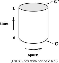
For illustration, we modify the definition of $\alpha_{\rm q\bar{q}}(q)$ to fit into this class of finite volume couplings. Consider the Yang-Mills theory on a $T\times L^{3}$ – torus with $T\gg L$. The finite volume coupling,

$$\tilde{\alpha}_{\rm q\bar{q}}(q) \equiv k\{r^{2}F(r,L)\}_{r=L/4}\,,\quad q=1/L\enspace,$$ (19)

can again be related to the $\overline{\rm MS}$ coupling perturbatively,

$$\tilde{\alpha}_{\rm q\bar{q}} = \alpha_{{\rm\overline{MS\kern-0.35002pt}\kern 0.35002pt}}+\tilde{c}_{1}^{\overline{\rm MS}\,\rm q\bar{q}}\alpha_{{\rm\overline{MS\kern-0.35002pt}\kern 0.35002pt}}^{2}+\ldots\enspace.$$ (20)

This relation may come as a surprise since it relates a small volume quantity to an infinite volume one. Remember, however, that once the bare coupling and masses are eliminated there are no free parameters. Renormalized couplings in finite volume and couplings in infinite volume are in one-to-one correspondence. When they are small they can be related by perturbation theory. In particular, (16) holds with the obvious modification.

The complete strategy to compute short distance parameters is summarized in Fig. 2.

$${L_{\rm max}}={\rm O}(\hbox{$1\over 2$}{\rm fm}):\qquad{\rm HS}\quad\longrightarrow\quad {\rm SF}(q=1/{L_{\rm max}})$$

$$\downarrow$$

$${\rm SF}(q=2/{L_{\rm max}})$$

$$\downarrow$$

$$\bullet$$

$$\bullet$$

$$\bullet$$

$$\downarrow$$

$${\rm SF}(q=2^{n}/{L_{\rm max}})$$

$$\mbox{ \small PT:}\quad\downarrow\qquad\quad$$

$${\rm jet-physics}\quad\stackrel{{\scriptstyle\rm PT}}{{\longleftarrow}}\quad \Lambda_{\rm QCD},M$$

Figure 2: The strategy for a non-perturbative computation of short distance parameters.

One first renormalizes QCD replacing the bare parameters by hadronic observables. This defines the hadronic scheme (HS) as explained in Sect. 1.1. At a low energy scale $q=1/L_{\rm max}$ this scheme can be related to the finite volume scheme denoted by SF in the graph. Within this scheme one then computes the scale evolution up to a desired energy $q=2^{n}/{L_{\rm max}}$. As we will see it is no problem to choose the number of steps $n$ large enough to be sure that one is in the perturbative regime. There perturbation theory (PT) is used to evolve further to infinite energy and compute the $\Lambda$-parameter and the renormalization group invariant quark masses. Inserted into perturbative expressions these provide predictions for jet cross sections or other high energy observables. In the graph all arrows correspond to relations in the continuum; the whole strategy is designed such that lattice calculations for these relations can be extrapolated to the continuum limit.

For the practical success of the approach, the finite volume coupling (as well as the corresponding quark mass) must satisfy a number of criteria.

• They should have an easy perturbative expansion, such that the $\beta$-function (and $\tau$-function, which describes the evolution of the running masses) can be computed to sufficient order.

• They should be easy to calculate in MC (small variance!).

• Discretization errors must be small to allow for safe extrapolations to the continuum limit.

Careful consideration of the above points led to the introduction of renormalized coupling and quark mass through the Schrödinger functional (SF) of QCD ([alphaII, alphaIII, StefanI, letter]). We introduce the SF in the following section. In the Yang-Mills theory, an alternative finite volume coupling was introduced in [alphaTPI] and studied in detail in [alphaTPII, alphaTPSF].

The criteria (17) apply quite generally to any scale dependent renormalization, e.g. the one described in Sect. 1.3 b. Although the details of the finite size technique have not yet been developed for these cases, the same strategy can be applied. This will certainly be the subject of future research. So far, the approach has been to search for a “window” where $q$ is high enough to apply PT but not too close to $a^{-1}$ ([renor_roma]). An essential advantage of the details of the approach of [renor_roma] as applied to the renormalization of composite quark operators is its simplicity: formulating the renormalization conditions in a MOM-scheme, one may use results from perturbation theory in infinite volume in the perturbative part of the matching. Since, however, high energies $q$ can not be reached in this approach, we will not discuss it further and refer to [renor_roma_appl, renor_roma_appl2] for an account of the present status and further references, instead. In particular, in the latter reference it can be seen, how non-trivial it is to have a “window” where both perturbation theory can be applied and lattice artifacts are small.

Note.

(17) has been written for the Yang-Mills theory. In full QCD, finite size effects will be more important and one should replace $\sqrt{K}\to m_{\pi}$, resulting in a more stringent requirement.

3 The Schrödinger functional

We want to introduce a specific finite volume scheme that fulfills all the requirements explained in the previous section. It is defined from the SF of QCD, which we introduce below. For simplicity we restrict the discussion to the pure gauge theory except for Sect. 3.7 and Sect. 3.8. Apart from the latter subsections, the presentation follows closely [alphaII]; we refer to this work for further details as well as proofs of the properties described below.

Figure 3: Illustration of the Schrödinger functional.

3.1 Definition

Here, we give a formal definition of the SF in the Yang-Mills theory in continuum space-time, noting that a rigorous treatment is possible in the lattice regularized theory.

Space-time is taken to be a cylinder illustrated in Fig. 3. We impose Dirichlet boundary conditions for the vector potentials in time,

$$A_{k}(x) = \left\{\begin{array}[]{ll}C_{k}^{\Lambda}({\bf x})&\mbox{at}\quad x_{0}=0\\ C^{\prime}_{k}({\bf x})&\mbox{at}\quad x_{0}=L\end{array}\right.\enspace,$$ (23)

where $C$, $C^{\prime}$ are classical gauge potentials and $A^{\Lambda}$ denotes the gauge transform of $A$,

$$A_{k}^{\Lambda}({\bf x}) = \Lambda({\bf x})A_{k}({\bf x})\Lambda({\bf x})^{-1}+\Lambda({\bf x})\partial_{k}\Lambda({\bf x})^{-1},\qquad\Lambda\in{\rm SU}(N)\enspace.$$ (24)

In space, we impose periodic boundary conditions,

$$A_{k}(x+L\hat{k}) = A_{k}(x),\qquad\Lambda({\bf x}+L\hat{k})=\Lambda({\bf x})\enspace.$$ (25)

The (Euclidean) partition function with these boundary conditions defines the SF,

$${{\cal Z}[C^{\prime},C]} \equiv \int{\rm D}[\Lambda]\int{\rm D}[A]\,{\rm e}^{-S_{\rm G}[A]}\enspace,$$ (26)

$$S_{\rm G}[A] = -{1\over 2g_{0}^{2}}\int{\rm d}^{4}x\,\,\hbox{tr}\,\left\{F_{\mu\nu}F_{\mu\nu}\right\},$$

$$F_{\mu\nu} = \partial_{\mu}A_{\nu}-\partial_{\nu}A_{\mu}+[A_{\mu},A_{\nu}]\enspace,$$

$$\qquad{\rm D}[A] = \prod_{{\bf x},\mu,a}{\rm d}A_{\mu}^{a}({x}),\qquad{\rm D}[\Lambda]=\prod_{\bf x}{\rm d}\Lambda({\bf x})\enspace.$$

Here ${\rm d}\Lambda({\bf x})$ denotes the Haar measure of ${\rm SU}(N)$. It is easy to show that the SF is a gauge invariant functional of the boundary fields,

$${\cal Z}[C^{\prime\Omega^{\prime}},C^{\Omega}]={\cal Z}[C^{\prime},C]\enspace,$$ (27)

where also large gauge transformations are permitted. The invariance under the latter is an automatic property of the SF defined on a lattice, while in the continuum formulation it is enforced by the integral over $\Lambda$ in (26).

3.2 Quantum mechanical interpretation

The SF is the quantum mechanical transition amplitude from a state $|C\rangle$ to a state $|C^{\prime}\rangle$ after a (Euclidean) time $L$. To explain the meaning of this statement of the SF, we introduce the Schrödinger representation. The Hilbert space consists of wave-functionals $\Psi[A]$ which are functionals of the spatial components of the vector potentials, $A_{k}^{a}({\bf x})$. The canonically conjugate field variables are represented by functional derivatives, $E_{k}^{a}({\bf x})={1\over i}{\delta\over\delta A_{k}^{a}({\bf x})}$, and a scalar product is given by

$$\langle\Psi|\Psi^{\prime}\rangle=\int{\rm D}[A]\,\Psi[A]^{*}\Psi^{\prime}[A],\qquad{\rm D}[A]=\prod_{{\bf x},k,a}{\rm d}A_{k}^{a}({\bf x})\enspace.$$ (28)

The Hamilton operator,

$$\mathchoice{\rm I\kern-1.4pt{H}}{\rm I\kern-1.4pt{H}}{\rm I\kern-1.1pt{H}}{\rm I\kern-1.1pt{H}}=\int_{0}^{L}{\rm d}^{3}x\,\left\{{g_{0}^{2}\over 2}E_{k}^{a}({\bf x})E_{k}^{a}({\bf x})+{1\over 4g_{0}^{2}}F_{kl}^{a}({\bf x})F_{kl}^{a}({\bf x})\right\}\enspace,$$ (29)

commutes with the projector, $\mathchoice{\rm I\kern-1.4pt{P}}{\rm I\kern-1.4pt{P}}{\rm I\kern-1.1pt{P}}{\rm I\kern-1.1pt{P}}$, onto the physical subspace of the Hilbert space (i.e. the space of gauge invariant states), where $\mathchoice{\rm I\kern-1.4pt{P}}{\rm I\kern-1.4pt{P}}{\rm I\kern-1.1pt{P}}{\rm I\kern-1.1pt{P}}$ acts as

$$\mathchoice{\rm I\kern-1.4pt{P}}{\rm I\kern-1.4pt{P}}{\rm I\kern-1.1pt{P}}{\rm I\kern-1.1pt{P}}\psi[A]=\int{\rm D}[\Lambda]\,\psi[A^{\Lambda}]\enspace.$$ (30)

Finally, each classical gauge field defines a state $|C\rangle$ through

$$\langle C|\Psi\rangle=\Psi[C]\enspace.$$ (31)

After these definitions, the quantum mechanical representation of the SF is given by

$${\cal Z}[C^{\prime},C] = \langle C^{\prime}|{\rm e}^{-\mathchoice{\rm I\kern-0.98pt{H}}{\rm I\kern-0.98pt{H}}{\rm I\kern-0.77pt{H}}{\rm I\kern-0.77pt{H}}T}\mathchoice{\rm I\kern-1.4pt{P}}{\rm I\kern-1.4pt{P}}{\rm I\kern-1.1pt{P}}{\rm I\kern-1.1pt{P}}|C\rangle$$ (32)

$$= \sum_{n=0}^{\infty}{\rm e}^{-E_{n}T}\Psi_{n}[C^{\prime}]\Psi_{n}[C]^{*}\enspace.$$

In the lattice formulation, (32) can be derived rigorously and is valid with real energy eigenvalues $E_{n}$.

3.3 Background field

A complementary aspect of the SF is that it allows a treatment of QCD in a color background field in an unambiguous way. Let us assume that we have a solution $B$ of the equations of motion, which satisfies also the boundary conditions (23). If, in addition,

$$S[A]>S[{B}]$$ (33)

for all gauge fields $A$ that are not equal to a gauge transform $B^{\Omega}$ of $B$, then we call $B$ the background field (induced by the boundary conditions). Here, $\Omega(x)$ is a gauge transformation defined for all $x$ in the cylinder and its boundary and $B^{\Omega}$ is the corresponding generalization of (24). Background fields $B$, satisfying these conditions are known; we will describe a particular family of fields, later.

Due to (33), fields close to $B$ dominate the path integral for weak coupling $g_{0}$ and the effective action,

$$\Gamma[B] \equiv -\ln{\cal Z}\left[C^{\prime},C\right]\enspace,$$ (34)

has a regular perturbative expansion,

$$\Gamma[B] = {1\over g_{0}^{2}}\Gamma_{0}[B]+\Gamma_{1}[B]+g_{0}^{2}\Gamma_{2}[B]+\ldots\enspace,$$ (35)

$$\Gamma_{0}[B] \equiv g_{0}^{2}S[B]\enspace.$$

Above we have used that due to our assumptions, the background field, $B$, and the boundary values $C,C^{\prime}$ are in one-to-one correspondence and have taken $B$ as the argument of $\Gamma$.

3.4 Perturbative expansion

For the construction of the SF-scheme as a renormalization scheme, one needs to study the renormalization properties of the functional, ${\cal Z}$. Lüscher et al. (1992) have performed a one-loop calculation for arbitrary background field. The calculation is done in dimensional regularization with $3-2\varepsilon$ space dimensions and one time dimension. One expands the field $A$ in terms of the background field and a fluctuation field, $q$, as

$$A_{\mu}(x)=B_{\mu}(x)+g_{0}q_{\mu}(x)\enspace.$$ (36)

Then one adds a gauge fixing term (“background field gauge”) and the corresponding Fadeev-Popov term. Of course, care must be taken about the proper boundary conditions in all these expressions. Integration over the quantum field and the ghost fields then gives

$$\Gamma_{1}[B]=\hbox{$1\over 2$}\ln\det\hat{\Delta}_{1}-\ln\det\hat{\Delta}_{0}\enspace,$$ (37)

where $\hat{\Delta}_{1}$ is the fluctuation operator and $\hat{\Delta}_{0}$ the Fadeev-Popov operator. The result can be cast in the form

$$\Gamma_{1}[B]\mathrel{\mathop{=}_{\varepsilon\to 0}} -{b_{0}\over\varepsilon}\,\Gamma_{0}[B]+{\rm O}(1)\enspace,$$ (38)

with the important result that the only (for $\varepsilon\to 0$) singular term is proportional to $\Gamma_{0}$.

After renormalization of the coupling, i.e. the replacement of the bare coupling by $\bar{g}_{{\rm\overline{MS\kern-0.35002pt}\kern 0.35002pt}}$ via

$$g_{0}^{2}= \bar{\mu}^{2\varepsilon}\bar{g}_{{\rm\overline{MS\kern-0.35002pt}\kern 0.35002pt}}^{2}(\mu)[1+z_{1}(\varepsilon)\bar{g}_{{\rm\overline{MS\kern-0.35002pt}\kern 0.35002pt}}^{2}(\mu)],\quad z_{1}(\varepsilon)=-{b_{0}\over\varepsilon}\enspace,$$ (39)

the effective action is finite,

$$\Gamma[B]_{\varepsilon=0} = \left\{{1\over\bar{g}_{{\rm\overline{MS\kern-0.35002pt}\kern 0.35002pt}}^{2}}-b_{0}\left[\ln\mu^{2}-\hbox{$1\over 16\pi^{2}$}\right]\right\}\Gamma_{0}[B]$$ (40)

$$-\hbox{$1\over 2$}\zeta^{\prime}(0|\Delta_{1})+\zeta^{\prime}(0|\Delta_{0})+{\rm O}(\bar{g}_{{\rm\overline{MS\kern-0.35002pt}\kern 0.35002pt}}^{2})$$

$$\zeta^{\prime}(0|\Delta) = \left.{{\rm d}\over{\rm d}s}\zeta(s|\Delta)\right|_{s=0},\qquad\zeta(s|\Delta)={\rm Tr}\,\Delta^{-s}\enspace.$$

Here, $\zeta^{\prime}(0|\Delta)$ is a complicated functional of $B$, which is not known analytically but can be evaluated numerically for specific choices of $B$.

The important result of this calculation is that (apart from field independent terms that have been dropped everywhere) the SF is finite after eliminating $g_{0}$ in favor of $\bar{g}_{{\rm\overline{MS\kern-0.35002pt}\kern 0.35002pt}}$. The presence of the boundaries does not introduce any extra divergences. In the following subsection we argue that this property is correct in general, not just in one-loop approximation.

3.5 General renormalization properties

The relevant question here is whether local quantum field theories formulated on space-time manifolds with boundaries develop divergences that are not present in the absence of boundaries (periodic boundary conditions or infinite space-time). In general the answer is “yes, such additional divergences exist”. In particular, Symanzik studied the $\phi^{4}$-theory with SF boundary conditions ([SymanzikSFI]). In a proof valid to all orders of perturbation theory he was able to show that the SF is finite after

• renormalization of the self-coupling, $\lambda$, and the mass, $m$,

• and the addition of the boundary counter-terms

  $$\int_{x^{0}=T}{\rm d}^{3}x\,\left\{Z_{1}\phi^{2}+Z_{2}\phi\partial_{0}\phi\right\}+\int_{x^{0}=0}{\rm d}^{3}x\,\left\{Z_{1}\phi^{2}-Z_{2}\phi\partial_{0}\phi\right\}\enspace.$$ (41)

In other words, in addition to the standard renormalizations, one has to add counter-terms formed by local composite fields integrated over the boundaries. One expects that in general, all fields with dimension $d\leq 3$ have to be taken into account. Already Symanzik conjectured that counter-terms with this property are sufficient to renormalize the SF of any quantum field theory in four dimensions.

Since this conjecture forms the basis for many applications of the SF to the study of renormalization, we note a few points concerning its status.

• As mentioned, a proof to all orders of perturbation theory exists for the $\phi^{4}$ theory, only.

• There is no gauge invariant local field with $d\leq 3$ in the Yang–Mills theory. Consequently no additional counter-term is necessary in accordance with the 1-loop result described in the previous subsection.

• In the Yang–Mills theory it has been checked also by explicit 2–loop calculations ([twoloop1, twoloop2]). Numerical, non-perturbative, MC simulations ([alphaIII, alphaTPSF]) give further support for its validity.

• It has been shown to be valid in QCD with quarks to 1-loop ([StefanI]).

• A straight forward application of power counting in momentum space in order to prove the conjecture is not possible due to the missing translation invariance.

Although a general proof is missing, there is little doubt that Symanzik’s conjecture is valid in general. Concerning QCD, this puts us into the position to give an elegant definition of a renormalized coupling in finite volume.

3.6 Renormalized coupling

For the definition of a running coupling we need a quantity which depends only on one scale. We choose $LB$ such that it depends only on one dimensionless variable $\eta$. In other words, the strength of the field is scaled as $1/L$. The background field is assumed to fulfill the requirements of Sect. 3.3. Then, following the above discussion, the derivative

$$\Gamma^{\prime}[B]={\partial\over\partial\eta}\Gamma[B]\enspace,$$ (42)

is finite when it is expressed in terms of a renormalized coupling like $\bar{g}_{{\rm\overline{MS\kern-0.35002pt}\kern 0.35002pt}}$ but $\Gamma^{\prime}$ is defined non-perturbatively. From (35) we read off immediately that a properly normalized coupling is given by

$$\bar{g}^{2}(L)=\Gamma^{\prime}_{0}[B]\bigm{/}\Gamma^{\prime}[B]\enspace.$$ (43)

Since there is only one length scale $L$, it is evident that $\bar{g}$ defined in this way runs with $L$.

A specific choice for the gauge group ${\rm SU(3)}$ is the abelian background field induced by the boundary values ([alphaIII])

$$C_{k}=\hbox{$i\over L$}\left(\begin{array}[]{ccc}\phi_{1}&0&0\\ 0&\phi_{2}&0\\ 0&0&\phi_{3}\end{array}\right)\,,\quad C^{\prime}_{k}=\hbox{$i\over L$}\left(\begin{array}[]{ccc}\phi^{\prime}_{1}&0&0\\ 0&\phi^{\prime}_{2}&0\\ 0&0&\phi^{\prime}_{3}\end{array}\right)\,,\quad k=1,2,3,$$ (50)

with

$$\begin{array}[]{lll}\phi_{1}=\eta-\hbox{$\pi\over 3$},&&\phi^{\prime}_{1}=-\phi_{1}-\hbox{$4\pi\over 3$},\\[4.30554pt] \phi_{2}=-\hbox{$1\over 2$}\eta,&&\phi^{\prime}_{2}=-\phi_{3}+\hbox{$2\pi\over 3$},\\[4.30554pt] \phi_{3}=-\hbox{$1\over 2$}\eta+\hbox{$\pi\over 3$},&&\phi^{\prime}_{3}=-\phi_{2}+\hbox{$2\pi\over 3$}.\end{array}$$ (54)

In this case, the derivatives with respect to $\eta$ are to be evaluated at $\eta=0$. The associated background field,

$$B_{0}=0,\qquad B_{k}=\left[x_{0}C_{k}^{\prime}+(L-x_{0})C_{k}\right]/L,\quad k=1,2,3\enspace,$$ (55)

has a field tensor with non-vanishing components

$$G_{0k}=\partial_{0}B_{k}=(C_{k}^{\prime}-C_{k})/L,\quad k=1,2,3\enspace.$$ (56)

It is a constant color-electric field.

3.7 Quarks

In the end, the real interest is in the renormalization of QCD and we need to consider the SF with quarks. It has been discussed in [StefanI].

Special care has to be taken in formulating the Dirichlet boundary conditions for the quark fields; since the Dirac operator is a first order differential operator, the Dirac equation has a unique solution when one half of the components of the fermion fields are specified on the boundaries. Indeed, a detailed investigation shows that the boundary condition

$$P_{+}\psi|_{x_{0}=0} = \rho,\quad P_{-}\psi|_{x_{0}=L}=\rho^{\prime}\,,\qquad P_{\pm}=\hbox{$1\over 2$}(1\pm\gamma_{0})\,,$$ (57)

$$\overline{\psi}P_{-}|_{x_{0}=0} = \bar{\rho},\quad\overline{\psi}P_{+}|_{x_{0}=L}=\bar{\rho}^{\prime}\,,$$ (58)

lead to a quantum mechanical interpretation analogous to (32). The SF

$${\cal Z}[C^{\prime},\bar{\rho}\kern 1.0pt^{\prime},\rho\kern 1.0pt^{\prime};C,\bar{\rho},\rho]=\int{\rm D}[A]{\rm D}[\,\psi\,]{\rm D}[\,\overline{\psi}\,]\,{\rm e}^{-S[A,\overline{\psi},\psi\,]}$$ (59)

involves an integration over all fields with the specified boundary values. The full action may be written as

$$S[A,\overline{\psi},\psi\,] = S_{\rm G}[\overline{\psi},\psi\,]+S_{\rm F}[A,\overline{\psi},\psi\,]$$

$$S_{\rm F} = \int{\rm d}^{4}x\,\overline{\psi}(x)[\gamma_{\mu}D_{\mu}+m]\psi(x)$$

$$-\int{\rm d}^{3}{\bf x}\,[\overline{\psi}(x)P_{-}\psi(x)]_{x_{0}=0}-\int{\rm d}^{3}{\bf x}\,[\overline{\psi}(x)P_{+}\psi(x)]_{x_{0}=L}\enspace,$$

with $S_{\rm G}$ as given in (26). In (3.7) we use standard Euclidean $\gamma$-matrices. The covariant derivative, $D_{\mu}$, acts as $D_{\mu}\psi(x)=\partial_{\mu}\psi(x)+A_{\mu}(x)\psi(x)$.

Let us now discuss the renormalization of the SF with quarks. In contrast to the pure Yang-Mills theory, gauge invariant composite fields of dimension three are present in QCD. Taking into account the boundary conditions one finds ([StefanI]) that the counter-terms,

$$\overline{\psi}P_{-}\psi|_{x_{0}=0}\,\,{\rm and}\,\,\overline{\psi}P_{+}\psi|_{x_{0}=L}\enspace,$$ (61)

have to be added to the action with weight $1-Z_{\rm b}$ to obtain a finite renormalized functional. These counter-terms are equivalent to a multiplicative renormalization of the boundary values,

$$\rho_{\rm R}=Z_{\rm b}^{-1/2}\rho\,,\,\,\ldots\,\,\,,\,\bar{\rho}^{\prime}_{\rm R}=Z_{\rm b}^{-1/2}\bar{\rho}^{\prime}\enspace.$$ (62)

It follows that – apart from the renormalization of the coupling and the quark mass – no additional renormalization of the SF is necessary for vanishing boundary values $\rho,\ldots,\bar{\rho}^{\prime}$. So, after imposing homogeneous boundary conditions for the fermion fields, a renormalized coupling may be defined as in the previous subsection.

As an important aside, we point out that the boundary conditions for the fermions introduce a gap into the spectrum of the Dirac operator (at least for weak couplings). One may hence simulate the lattice SF for vanishing physical quark masses. It is then convenient to supplement the definition of the renormalized coupling by the requirement $m=0$. In this way, one defines a mass-independent renormalization scheme with simple renormalization group equations. In particular, the $\beta$-function remains independent of the quark mass.

3.7.1 Correlation functions

are given in terms of the expectation values of any product $\cal O$ of fields,

$$\langle{\cal O}\rangle=\left\{{1\over{\cal Z}}\int{\rm D}[A]{\rm D}[\,\psi\,]{\rm D}[\,\overline{\psi}\,]\,{\cal O}\,{\rm e}^{-S[A,\overline{\psi},\psi\,]}\right\}_{\bar{\rho}\kern 1.0pt^{\prime}=\rho\kern 1.0pt^{\prime}=\bar{\rho}=\rho=0}\enspace,$$ (63)

evaluated for vanishing boundary values $\rho,\ldots,\bar{\rho}^{\prime}$. Apart from the gauge field and the quark and anti-quark fields integrated over, $\cal O$ may involve the “boundary fields” ([paper1])

$$\zeta({\bf x}) = {\delta\over\delta\bar{\rho}({\bf x})},\qquad\bar{\zeta}({\bf x})=-{\delta\over\delta\rho({\bf x})},$$

$$\zeta^{\prime}({\bf x}) = {\delta\over\delta\bar{\rho}\kern 1.0pt^{\prime}({\bf x})},\qquad\bar{\zeta}\kern 1.0pt^{\prime}({\bf x})=-{\delta\over\delta\rho\kern 1.0pt^{\prime}({\bf x})}\enspace.$$ (64)

An application of fermionic correlation functions including the boundary fields is the definition of the renormalized quark mass in the SF scheme to be discussed next.

3.8 Renormalized mass

Just as in the case of the coupling constant, there is a great freedom in defining renormalized quark masses. A natural starting point is the PCAC relation which expresses the divergence of the axial current (5) in terms of the associated pseudo-scalar density,

$$P^{a}(x) = \overline{\psi}(x)\gamma_{5}\hbox{$1\over 2$}\tau^{a}\psi(x)\enspace,$$ (65)

via

$$\partial_{\mu}A_{\mu}^{a}(x)=2mP^{a}(x)\enspace.$$ (66)

This operator identity is easily derived at the classical level (cf. Sect. 6). After renormalizing the operators,

$$(A_{{\rm R}})_{\mu}^{a} = Z_{\rm A}A_{\mu}^{a}\enspace,$$

$$P_{{\rm R}}^{a} = Z_{\rm P}P^{a}\enspace,$$ (67)

a renormalized current quark mass may be defined by

$$\kern 1.0pt\overline{\kern-1.0ptm\kern-1.0pt}\kern 1.0pt={Z_{\rm A}\over Z_{\rm P}}m\enspace.$$ (68)

Here, $m$, is to be taken from (66) inserted into an arbitrary correlation function and $Z_{\rm A}$ can be determined unambiguously as mentioned in Sect. 1.2. Note that $m$ does not depend on which correlation function is used because the PCAC relation is an operator identity. The definition of $\kern 1.0pt\overline{\kern-1.0ptm\kern-1.0pt}\kern 1.0pt$ is completed by supplementing (67) with a specific normalization condition for the pseudo-scalar density. $\kern 1.0pt\overline{\kern-1.0ptm\kern-1.0pt}\kern 1.0pt$ then inherits its scheme- and scale-dependence from the corresponding dependence of $P_{{\rm R}}$. Such a normalization condition may be imposed through infinite volume correlation functions. Since we want to be able to compute the running mass for large energy scales, we do, however, need a finite volume definition. This is readily given in terms of correlation functions in the SF.

Figure 4: $f_{\rm P}$ (left) and $f_{1}$ (right) in terms of quark propagators.

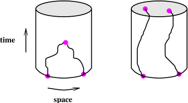
To start with, let us define (isovector) pseudo-scalar fields at the boundary of the SF,

$${\cal O}^{a} = \int{\rm d}^{3}{\bf u}\int{\rm d}^{3}{\bf v}\,\,\bar{\zeta}({\bf u})\gamma_{5}\hbox{$1\over 2$}\tau^{a}\zeta({\bf v}),$$

$${\cal O}\kern-7.7778pt\kern 7.7778pt\smash{\raise 4.5pt\hbox{\kern 1.0pt$\scriptstyle\prime$}}\kern 1.0pt^{a} = \int{\rm d}^{3}{\bf u}\int{\rm d}^{3}{\bf v}\,\,\bar{\zeta}\kern 1.0pt^{\prime}({\bf u})\gamma_{5}\hbox{$1\over 2$}\tau^{a}\zeta^{\prime}({\bf v})\enspace,$$ (69)

to build up the correlation functions

$$f_{\rm P}(x_{0}) = -\hbox{$1\over 3$}\langle P^{a}(x){\cal O}^{a}\rangle\enspace,$$

$$f_{1} = \langle{\cal O}\kern-7.7778pt\kern 7.7778pt\smash{\raise 4.5pt\hbox{\kern 1.0pt$\scriptstyle\prime$}}\kern 1.0pt^{a}{\cal O}^{a}\rangle\enspace,$$ (70)

which are illustrated in Fig. 4.

We then form the ratio

$$Z_{\rm P}={\rm const.}\sqrt{f_{1}}/f_{\rm P}(x)|_{x_{0}=L/2}\enspace,$$ (71)

such that the renormalization of the boundary quark fields, (62), cancels out. The proportionality constant is to be chosen such that $Z_{\rm P}=1$ at tree level. To define the scheme completely one needs to further specify the boundary values $C,C^{\prime}$ and the boundary conditions for the quark fields in space. These details are of no importance, here.

We rather mention some more basic points about this renormalization scheme. Just like in the case of the running coupling, the only physical scale that exists in our definitions (68),(71) is the linear dimension of the SF, the length scale, $L$. So the mass $\kern 1.0pt\overline{\kern-1.0ptm\kern-1.0pt}\kern 1.0pt(L)$ runs with $L$. We have already emphasized that $\bar{g}$ is to be evaluated at zero quark mass. It is advantageous to do the same for $Z_{\rm P}$. In this way we define a mass-independent renormalization scheme, with simple renormalization group equations.

By construction, the SF scheme is non-perturbative and independent of a specific regularization. For a concrete non-perturbative computation, we do, however, need to evaluate the expectation values by a MC-simulation of the corresponding lattice theory. We proceed to introduce the lattice formulation of the SF.

3.9 Lattice formulation

A detailed knowledge of the form of the lattice action is not required for an understanding of the following sections. Nevertheless, we give a definition of the SF in lattice regularization. This is done both for completeness and because it allows us to obtain a first impression about the size of discretization errors.

We choose a hyper-cubic Euclidean lattice with spacing $a$. A gauge field $U$ on the lattice is an assignment of a matrix $U(x,\mu)\in{\rm SU}(N)$ to every lattice point $x$ and direction $\mu=0,1,2,3$. Quark and anti-quark fields, $\psi(x)$ and $\overline{\psi}(x)$, reside on the lattice sites and carry Dirac, color and flavor indices as in the continuum. To be able to write the quark action in an elegant form it is useful to extend the fields, initially defined only inside the SF manifold (cf. Fig. 3) to all times $x_{0}$ by “padding” with zeros. In the case of the quark field one sets

$$\psi(x)=0\quad\hbox{if $x_{0}<0$ or $x_{0}>L$},$$

and

$$P_{-}\psi(x)|_{x_{0}=0}=P_{+}\psi(x)|_{x_{0}=L}=0,$$

and similarly for the anti-quark field. Gauge field variables that reside outside the manifold are set to 1.

We may then write the fermionic action as a sum over all space-time points without restrictions for the time-coordinate,

$$S_{\rm F}[U,\bar{\psi},\psi] = a^{4}\sum_{x}\bar{\psi}(D+m_{0})\psi,$$ (72)

and with the standard Wilson-Dirac operator,

$$D=\hbox{$1\over 2$}\sum_{\mu=0}^{3}\{\gamma_{\mu}(\nabla_{\mu}^{\ast}+\nabla_{\mu})-a\nabla_{\mu}^{\ast}\nabla_{\mu}\}\,.$$ (73)

Here, forward and backward covariant derivatives,

$$\nabla_{\mu}\psi(x) = \hbox{$1\over a$}[U(x,\mu)\psi(x+a\hat{\mu})-\psi(x)],$$ (74)

$$\nabla_{\mu}^{\ast}\psi(x) = \hbox{$1\over a$}[\psi(x)-U(x-a\hat{\mu},\mu)^{-1}\psi(x-a\hat{\mu})]\enspace,$$ (75)

are used and $m_{0}$ is to be understood as a diagonal matrix in flavor space with elements $m_{0}^{f}$.

The gauge field action $S_{\rm G}$ is a sum over all oriented plaquettes $p$ on the lattice, with the weight factors $w(p)$, and the parallel transporters $U(p)$ around $p$,

$$S_{\rm G}[U]={1\over g_{0}^{2}}\sum_{p}w(p)\,\,\hbox{tr}\,\{1-U(p)\}\enspace.$$ (76)

The weights $w(p)$ are 1 for plaquettes in the interior and

$$w(p)=\left\{\begin{array}[]{ll}{\scriptstyle\hbox{$1\over 2$}}c_{s}&\mbox{if $p$ is a spatial plaquette at $x_{0}=0$ or $x_{0}=L$},\\ c_{t}&\mbox{if $p$ is time-like and attached to a boundary plane.}\end{array}\right.$$ (77)

The choice $c_{s}=c_{t}=1$ corresponds to the standard Wilson action. However, these parameters can be tuned in order to reduce lattice artifacts, as will be briefly discussed below.

With these ingredients, the path integral representation of the Schrödinger functional reads ([StefanI]),

$${\cal Z} = \int{\rm D}[\psi]{\rm D}[\bar{\psi}\,]{\rm D}[U]\,{\rm e}^{-S}\,,\quad S=S_{\rm F}+S_{\rm G}\enspace,$$

$${\rm D}[U]=\prod_{x,\mu}{\rm d}U(x,\mu)\enspace,$$

with the Haar measure ${\rm d}U$.

3.9.1 Boundary conditions and the background field.

The boundary conditions for the lattice gauge fields may be obtained from the continuum boundary values by forming the appropriate parallel transporters from $x+a\hat{k}$ to $x$ at $x_{0}=0$ and $x_{0}=L$. For the constant abelian boundary fields $C$ and $C^{\prime}$ that we considered before, they are simply

$$U(x,k)|_{x_{0}=0}=\exp(aC_{k}),\qquad U(x,k)|_{x_{0}=L}=\exp(aC^{\prime}_{k}),$$ (79)

for $k=1,2,3$. All other boundary conditions are as in the continuum.

For the case of (50),(54), the boundary conditions (79) lead to a unique (up to gauge transformations) minimal action configuration $V$, the lattice background field. It can be expressed in terms of $B$ (55),

$$V(x,\mu)=\exp\left\{aB_{\mu}(x)\right\}\enspace.$$ (80)

3.9.2 Lattice artifacts.

Now we want to get a first impression about the dependence of the lattice SF on the value of the lattice spacing. In other words we study lattice artifacts. At lowest order in the bare coupling we have, just like in the continuum,

$$\Gamma={1\over g_{0}^{2}}\Gamma_{0}[V]+{\rm O}((g_{0})^{0})\,,\quad\Gamma_{0}[V]\equiv g_{0}^{2}S_{\rm G}[V]\enspace.$$ (81)

Furthermore one easily finds the action for small lattice spacings,

$$S_{\rm G}[V] = \left[1+(1-c_{\rm t})\hbox{$2a\over L$}\right]{3L^{4}\over g_{0}^{2}}\sum_{\alpha=1}^{N}\left\{{2\over a^{2}}\sin\left[{a^{2}\over 2L^{2}}\left(\phi^{\prime}_{\alpha}-\phi_{\alpha}\right)\right]\right\}^{2}$$ (82)

$$= {3\over g_{0}^{2}}\sum_{\alpha=1}^{N}\left(\phi^{\prime}_{\alpha}-\phi_{\alpha}\right)^{2}\left[1+(1-c_{\rm t}){\hbox{$2a\over L$}+{\rm O}(a^{4})}\right]\enspace.$$

We observe: at tree-level of perturbation theory, all linear lattice artifacts are removed when one sets $c_{\rm t}=1$. Beyond tree-level, one has to tune the coefficient $c_{\rm t}$ as a function of the bare coupling. We will show the effect, when this is done to first order in $g_{0}^{2}$, below. Note that the existence of linear ${\rm O}(a)$ errors in the Yang-Mills theory is special to the SF; they originate from dimension four operators $F_{0k}F_{0k}$ and $F_{kl}F_{kl}$ which are irrelevant terms (i.e. they carry an explicit factor of the lattice spacing) when they are integrated over the surfaces. $c_{\rm s}$, which can be tuned to cancel the effects of $F_{kl}F_{kl}$, does not appear for the electric field that we discussed above.

Once quark fields are present, there are more irrelevant operators that can generate ${\rm O}(a)$ effects as discussed in detail in [paper1]. Here we emphasize a different feature of (82): once the ${\rm O}(a)$-terms are canceled, the remaining $a$-effects are tiny. This special feature of the abelian background field is most welcome for the numerical computation of the running coupling; it allows for reliable extrapolations to the continuum limit.

3.9.3 Explicit expression for $\Gamma^{\prime}$.

Let us finally explain that $\Gamma^{\prime}$ is an observable that can easily be calculated in a MC simulation. From its definition we find immediately

$${\Gamma^{\prime}} = -{\partial\over\partial\eta}\ln\left\{\int{{\rm D}[\psi]{\rm D}[\bar{\psi}\,]{\rm D}[U]\,{\rm e}^{-S}}\right\}=\left\langle{\partial S\over\partial\eta}\right\rangle\enspace.$$ (83)

The derivative $\partial S\over\partial\eta$ evaluates to the (color 8 component of the) electric field at the boundary,

$${\partial S\over\partial\eta} = -{2\over g_{0}^{2}\,L}a^{3}\sum_{\bf x}\left\{E_{k}^{8}({\bf x})-(E_{k}^{8})^{\prime}({\bf x})\right\}\enspace,$$ (84)

$$E_{k}^{8}({\bf x}) = {1\over a^{2}}{\rm Re}\,\,\hbox{tr}\,\left\{i\lambda_{8}U(x,k)U(x+a\hat{k},0)U(x+a\hat{0},k)^{-1}U(x,0)^{-1}\right\}_{x_{0}=0}\enspace,$$

where $\lambda_{8}={\rm diag}(1,-1/2,-1/2)$. (A similar expression holds for $(E_{k}^{8})^{\prime}({\bf x})$). The renormalized coupling is therefore given in terms of the expectation value of a local operator; no correlation function is involved. This means that it is easy and fast in computer time to evaluate it. It further turns out that a good statistical precision is reached with a moderate size statistical ensemble.

4 The computation of $\alpha(q)$

We are now in the position to explain the details of Fig. 2 ([alphaI, alphaIII, lat97]). The problem has been solved in the SU(3) Yang-Mills theory. In the present context, this is of course equivalent to the quenched approximation of QCD or the limit of zero flavors. We will therefore also refer to results in quenched QCD.

Our central observable is the step scaling function that describes the scale-evolution of the coupling, i.e. moving vertically in Fig. 2. The analogous function for the running quark mass will be discussed in the following section.

4.1 The step scaling function

Figure 5: Schematic plot of the running coupling constructed from the step scaling function $\sigma$.

We start from a given value of the coupling, $u=\bar{g}^{2}(L)$. When we change the length scale by a factor $s$, the coupling has a value $\bar{g}^{2}(sL)=u^{\prime}$ . The step scaling function, $\sigma$ is then defined as

$$\sigma(s,u) = u^{\prime}\enspace.$$ (85)

The interpretation is obvious. $\sigma(s,u)$ is a discrete $\beta$-function. Its knowledge allows for the recursive construction of the running coupling at discrete values of the length scale,

$$u_{k}=\bar{g}^{2}(s^{-k}L)\enspace,$$ (86)

once a starting value $u_{0}=\bar{g}^{2}(L)$ is specified (cf. Fig. 5). $\sigma$, which is readily expressed as an integral of the $\beta$-function, has a perturbative expansion

$$\sigma(s,u) = u+2b_{0}\ln(s)u^{2}+\ldots\enspace.$$ (87)

On a lattice with finite spacing, $a$, the step scaling function will have an additional dependence on the resolution $a/L$. We define

$$\Sigma(s,u,a/L) = u^{\prime}\enspace,$$ (88)

with

$$\bar{g}^{2}(L) = u,\quad\bar{g}^{2}(sL)=u^{\prime}\,,\quad\mbox{$g_{0}$ fixed, $L/a$ fixed}\enspace.$$ (89)

The continuum limit $\sigma(s,u)=\Sigma(s,u,0)$ is then reached by performing calculations for several different resolutions and extrapolation $a/L\to 0$. In detail, one performs the following steps:

• Choose a lattice with $L/a$ points in each direction.

• Tune the bare coupling $g_{0}$ such that the renormalized coupling $\bar{g}^{2}(L)$ has the value $u$.

• At the same value of $g_{0}$, simulate a lattice with twice the linear size; compute $u^{\prime}=\bar{g}^{2}(2L)$. This determines the lattice step scaling function $\Sigma(2,u,a/L)$.

• Repeat steps 1.–3. with different resolutions $L/a$ and extrapolate $a/L\to 0$.

Note that step 2. takes care of the renormalization and 3. determines the evolution of the renormalized coupling.

Sample numerical results are displayed in Fig. 6. The coupling used is exactly the one defined in the previous section and the calculation is done in the theory without fermions. One observes that the dependence on the resolution is very weak, in fact it is not observable with the precision of the data in Fig. 6. We now investigate in more detail how the continuum limit of $\Sigma$ is reached. As a first step, we turn to perturbation theory.

Figure 6: Typical example for the lattice step scaling function after 1-loop improvement. The continuum limit (circle) is reached by linear extrapolation.

4.2 Lattice spacing effects in perturbation theory

Symanzik has investigated the cutoff dependence of field theories in perturbation theory ([Symanzik]). Generalizing his discussion to the present case, one concludes that the lattice spacing effects have the expansion

$${\Sigma(2,u,a/L)-\sigma(2,u)\over\sigma(2,u)} = \delta_{1}(a/L)\,u+\delta_{2}(a/L)\,u^{2}+\ldots$$ (90)

$$\delta_{n}(a/L) {\buildrel{a/L}\rightarrow 0\over{\sim}} \sum_{k=0}^{n}e_{k,n}[\ln(\hbox{$a\over L$})]^{k}{\left(\hbox{$a\over L$}\right)}+d_{k,n}[\ln(\hbox{$a\over L$})]^{k}{\left(\hbox{$a\over L$}\right)^{2}}+\ldots\enspace.$$

We expect that the continuum limit is reached with corrections ${\rm O}(a/L)$ also beyond perturbation theory. In this context ${\rm O}(a/L)$ summarizes terms that contain at least one power of $a/L$ and may be modified by logarithmic corrections as it is the case in (90). To motivate this expectation recall Sect. 1.4, where we explained that lattice artifacts correspond to irrelevant operators, which carry explicit factors of the lattice spacing. Of course, an additional $a$-dependence comes from their anomalous dimension, but in an asymptotically free theory such as QCD, this just corresponds to a logarithmic (in $a$) modification.

Figure 7: Lattice artifacts at 1-loop order. The circles show $\delta_{1}(a/L)$ for the SU(3) Yang-Mills theory with 1-loop improvement. The dotted line corresponds to the linear piece in $a$, when only tree-level improvement is used, instead.

As mentioned in the previous section, the lattice artifacts may be reduced to ${\rm O}((a/L)^{2})$ by canceling the leading irrelevant operators. In the case at hand, this is achieved by a proper choice of $c_{\rm t}(g_{0})$. It is interesting to note, that by using the perturbative approximation

$$c_{\rm t}(g_{0})=1+c_{\rm t}^{(1)}g_{0}^{2}$$ (91)

one does not only eliminate $e_{1,n}$ for $n=0,1$ but also the logarithmic terms generated at higher orders are reduced,

$$e_{n,n}=0,\quad e_{n-1,n}=0\enspace.$$ (92)

For tree-level improvement, $c_{\rm t}(g_{0})=1$, the corresponding statement is $e_{n,n}=0$. Heuristically, the latter is easy to understand. Tree-level improvement means that the propagators and vertices agree with the continuum ones up to corrections of order ${\rm O}(a^{2})$. Terms proportional to $a$ can then arise only through a linear divergence of the Feynman diagrams. Once this happens, one cannot have the maximum number of logarithmic divergences any more; consequently $e_{n,n}$ vanishes.

To demonstrate further that the abelian field introduced in the previous section induces small lattice artifacts, we show $\delta_{1}(a/L)$ for the one loop improved case. The term that is canceled by the proper choice $c_{\rm t}^{(1)}=-0.089$ is shown as a dashed line. The left over ${\rm O}((a/L)^{2})$-terms are below the 1% level for couplings $u\leq 2$ and lattice sizes $L/a\geq 6$. We now understand better why the $a/L$-dependence is so small in Fig. 6.

From the investigation of lattice spacing effects in perturbation theory one expects that one may safely extrapolate to the continuum limit by a fit

$$\Sigma(2,u,a/L)=\sigma(2,u)+{\rm const.}\times a/L\enspace,$$ (93)

once one has data with a weak dependence on $a/L$, like the ones in Fig. 6. Such an extrapolation is shown in the figure.

4.3 The continuum limit – universality

Figure 8: Universality test in the SU(2) Yang Mills theory.

Before proceeding with the extraction of the running coupling, we present some further examples of numerical investigations of the approach to the continuum limit – and its very existence ([alphaIII, alphaTPSF]). The first example is the step scaling function in the SU(2) Yang-Mills theory ([alphaTPSF]). Here we can compare the step scaling function obtained with two different lattice actions, one using tree-level ${\rm O}(a)$ improvement and the other one using $c_{\rm t}$ at 1-loop order. (Fig. 8).

Not only does one observe a substantial reduction of the ${\rm O}(a)$-errors through perturbative improvement, but the very agreement of the two calculations when extrapolated to $a=0$, leaves little doubt that the continuum limit of the SF exists and is independent of the lattice action. In turn this also supports the statement that the SF is renormalized after the renormalization of the coupling constant.

Turning attention back to the gauge group SU(3), we show the calculation of $\sigma(2,u)$ for a whole series of couplings $u$ in Fig. 9.

Figure 9: Continuum extrapolation of $\sigma(2,u)$ in the SU(3) Yang-Mills theory.

4.4 The running of the coupling

Figure 10: The running coupling in SU(3) Yang-Mills theory. Uncertainties are smaller than the size of the symbols.

We may now use the continuum step scaling function to compute a series of couplings (86). We start at the largest value of the coupling that was covered by the calculation: $\bar{g}^{2}=3.48$. This defines the largest value of the box size, $L_{\rm max}$,

$$\bar{g}^{2}(L_{\rm max})=3.48\enspace.$$ (94)

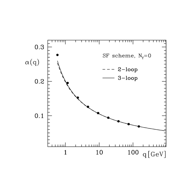
The series of couplings is then obtained for $L_{k}=2^{-k}L_{\rm max},\,k=0,1,\ldots 8$. It is shown in Fig. 10 translated to $\alpha(q)=\bar{g}^{2}(L)/(4\pi),\,\,q=1/L$ (We will explain below, how one arrives at a ${\rm GeV}$-scale in this plot). The range of couplings shown in the figure is the range covered in the non-perturbative calculation of the step scaling function. Thus no approximations are involved. For comparison, the perturbative evolution is shown starting at the smallest value of $\alpha$ that was reached. To be precise, 2-loop accuracy here means that we truncate the $\beta$-function at 2 loops and integrate the resulting renormalization group equation exactly. Thanks to the recent work ([twoloop2, twoloop3]), we can also compare to the 3-loop evolution of the coupling.

It is surprising that the perturbative evolution is so precise down to very low energy scales. This property may of course not be generalized to other schemes, in particular not to the $\overline{\rm MS}$-scheme, where the $\beta$-function is only defined in perturbation theory, anyhow.

4.5 The low energy scale

In order to have the coupling as a function of the energy scale in physical units, we need to know $L_{\rm max}$ in ${\rm fm}$, the first horizontal relation in Fig. 2. In QCD, this should be done by computing, for example, the product $m_{\rm p}L_{\rm max}$ with $m_{\rm p}$ the proton mass and then inserting the experimentally determined value of the proton mass.

At present, results like the ones shown in Fig. 10 are available for the Yang-Mills theory, only. Therefore, strictly speaking, there is no experimental observable to take over the role of the proton mass. As a purely theoretical exercise, one could replace the proton mass by a glueball mass; here, we choose a length scale, $r_{0}$, derived from the force between static quarks, instead ([r0paper]). This quantity can be computed with better precision. Also one may argue that the static force is less influenced by whether one has dynamical quark loops in the theory or not.

Figure 11: The dimensionless combination $r^{2}F(r)$. The different curves show phenomenologically successful potential models ([Cornell, Martin, Quigg-Rosner]). The labels on the top of the graph give the approximate values of the r.m.s-radii of the bound states.

On the theoretical level, $r_{0}$, has a precise definition. One evaluates the force $F(r)$ between an external, static, quark–anti-quark pair as a function of the distance $r$. The radius $r_{0}$ is then implicitly defined by

$$r^{2}F(r)|_{r=r_{0}}=1.65\enspace.$$ (95)

On the other hand, to obtain a phenomenological value for $r_{0}$, one needs to assume an approximate validity of potential models for the description of the spectra of $c\bar{c}$ and $b\bar{b}$ mesons. This is illustrated in Fig. 11. In fact, the value $1.65$ on the r.h.s. of (95) has been chosen to have $r_{0}=0.5\,{\rm fm}$ from the Cornell potential. This is a distance which is well within the range where the observed bound states determine (approximately) the phenomenological potential.

Figure 12: Continuum extrapolation of $L_{\rm max}/r_{0}$, using data of [UKQCDr0, alphaIII].

In the following we set $r_{0}=0.5\,{\rm fm}$, emphasizing that this is mainly for the purpose of illustration and should be replaced by a direct experimental observable once one computes the coupling in full QCD.

To obtain $L_{\rm max}/r_{0}$ from lattice QCD, one picks a certain value of $L/a$, tunes the bare coupling $g_{0}$ such that $\bar{g}^{2}=3.48$. At the same value of $g_{0}$ one then computes the force $F(r)$ on a lattice that is large enough such that finite size effects are negligible for the calculation of $F(r)$ and determines $r_{0}$. Repeating the calculation for various values of $L/a$ one may extrapolate the lattice results to zero lattice spacing (Fig. 12) and can quote the energies $q$ in ${\rm GeV}$, as done in Fig. 10.

4.6 Matching at finite energy

Following the strategy of Fig. 2, one finally computes the $\Lambda$-parameter in the SF scheme. It may be converted to any other scheme through a 1-loop calculation. There is no perturbative error in this relation, as the $\Lambda$-parameter refers to infinite energy, where $\alpha$ is arbitrarily small.

Nevertheless, in order to clearly explain the problem, we first consider changing schemes perturbatively at a finite but large value of the energy. Before writing down the perturbative relation between $\alpha_{X}$ and $\alpha_{Y}$ where $X,Y$ label the schemes, we note that in any scheme, there is an ambiguity in the energy scale $q$ used as argument for $\alpha$. For example in the SF-scheme, we have set $q=1/L$, but a choice $q=\pi/L$ would have been possible as well. This suggests immediately to allow for the freedom to compare the couplings after a relative energy shift. So we introduce a scale factor $s$ in the perturbative relation,

$$\alpha_{Y}({s}q)=\alpha_{X}(q)+c_{1}^{XY}({s})[\alpha_{X}(q)]^{2}+c_{2}^{XY}({s})[\alpha_{X}(q)]^{3}+\ldots\enspace.$$ (96)

A natural and non-trivial question is now, which scale ratio $s$ is optimal. A possible criterion is to choose $s$ such that the available terms in the perturbative series (96) are as small as possible. Since the number of available terms in the series is usually low, we concentrate here on the possibility to set the first non-trivial term to zero. When available, the higher order one(s) may be used to test the success of this procedure.

Scheme $X$	$c_{1}^{X~{}\overline{\rm MS}}(1)$	$c_{2}^{X~{}\overline{\rm MS}}(1)$	$c_{2}^{X~{}\overline{\rm MS}}({s_{0}})$
$q\bar{q}$	$-0.0821$	$-2.24$	$-2.19$
SF	$1.256$	$2.775$	$0.27$
SF  SU(2)	0.943	$1.411$	$0.058$
TP  SU(2)	$-0.558$

Table 1: Examples for perturbative coefficients in (96) for $N_{\rm f}=0$.

So we fix $s$ by requiring $c_{1}^{XY}(s)=0$ , which is satisfied for $s=s_{0}$ with

$$s_{0} = \exp\{-c_{1}^{XY}(1)/(8\pi b_{0})\}=\Lambda_{X}/\Lambda_{Y},$$ (97)

a relative shift given by the ratio of the $\Lambda$-parameters in the two schemes. Examples taken from the literature ([alphaII, alphaIII, twoloop1, twoloop2, twoloop3, qqbar1loop1, oneloopferm, qqbar1loop2, qqbar2loop]) are listed in Table 1. In the case of matching the SF-scheme to $\overline{\rm MS}$, the use of $s_{0}$ does indeed reduce the 2-loop coefficient considerably. However for the $q\bar{q}$-scheme $s_{0}$ is close to one and the 2-loop coefficient remains quite big. Not too surprisingly, no universal success of (97) is seen.

A non-perturbative test of the perturbative matching has been carried out by [alphaTPSF] in the SU(2) Yang-Mills theory, where the SF-scheme was related to a different finite volume scheme, called TP. The matching coefficient for this case is also listed in Table 1. Non-perturbatively the matching was computed as follows.

• For fixed $L/a$, the bare coupling was tuned such that $\bar{g}^{2}_{\rm SF}(L)=2.0778$ (or equivalently $\alpha_{\rm SF}(q=1/L)=0.1653$).

• At the same bare coupling $\bar{g}^{2}_{\rm TP}(L)$ was computed.

• These steps were repeated for a range of $a/L$ and the results for $\bar{g}^{2}_{\rm TP}(L)$ were extrapolated to the continuum.

The result is shown in Fig. 13.

Figure 13: Non-perturbative test of perturbative matching.

We observe that a naive application of the 1-loop formula with $s=1$ falls far short of the non-perturbative number (the point with error bar), while inserting $s=s_{0}$ gives a perturbative estimate which is close to the true answer. Indeed, the left over difference is roughly of a magnitude $\alpha^{3}$.

Nevertheless, without the non-perturbative result, the error inherent in the perturbative matching is rather difficult to estimate. For this reason it is very attractive to perform the matching at infinite energies, i.e. through the $\Lambda$–parameters, where no perturbative error remains.

4.7 The $\Lambda$ parameter of quenched QCD

We first note that the $\Lambda$-parameter in a given scheme is just the integration constant in the solution of the renormalization group equation. This is expressed by the exact relation

$$\Lambda = q\left(b_{0}\bar{g}^{2}\right)^{-b1/(2b_{0}^{2})}{\rm e}^{-1/(2b_{0}\bar{g}^{2})}\exp\left\{-\int_{0}^{\bar{g}}{\rm d}x\left[\hbox{$1\over\beta(x)$}+\hbox{$1\over b_{0}x^{3}$}-\hbox{$b_{1}\over b_{0}^{2}x$}\right]\right\}\enspace.$$ (98)

We may evaluate this expression for the last few data points in Fig. 10 using the 3-loop approximation to the $\beta$-function in the SF-scheme. The resulting $\Lambda$-values are essentially independent of the starting point, since the data follow the perturbative running very accurately. This excludes a sizeable contribution to the $\beta$-function beyond 3-loops and indeed, a typical estimate of a 4-loop term in the $\beta$-function would change the value of $\Lambda$ by a tiny amount. The corresponding uncertainty can be neglected compared to the statistical errors.

After converting to the $\overline{\rm MS}$-scheme one arrives at the result ([lat97])

$$\Lambda_{\overline{\rm MS}}^{(0)}=251\pm 21{\rm MeV}\enspace,$$ (99)

where the label ⁽⁰⁾ reminds us that this number was obtained with zero quark flavors, i.e. in the Yang-Mills theory. Since this is not the physical theory, one must also remember that the overall scale of the theory was set by putting $r_{0}=0.5\,{\rm fm}$. We emphasize that the error in (99) sums up all errors including the extrapolations to the continuum limit that were done in the various intermediate steps.

4.8 The use of bare couplings

As mentioned before, the recursive finite size technique has not yet been applied to QCD with quarks. Instead, $\alpha_{\overline{\rm MS}}$ has been estimated through lattice gauge theories by using a short cut, namely the relation between the bare coupling of the lattice theory and the $\overline{\rm MS}$-coupling at a physical momentum scale which is of the order of the inverse lattice spacing that corresponds to the bare coupling ([fermilab]). Without going too much into details, we want to discuss this approach, its merits and its shortcomings, here. The emphasis is on the principle and not on the applications, which can be found in [alpha_dyn]. So, although the main point is to be able to include quarks, we set $N_{\rm f}=0$ in the discussion; more is known in this case!

The method simply requires that one computes one dimensionful experimental observable in lattice QCD at a certain value of the bare coupling $g_{0}$. A popular choice for this is a mass splitting in the $\Upsilon$-system ([Davies]). Using as input the experimental mass splitting one determines the lattice spacing in physical units.

Next one may attempt to use the perturbative relation,

$$\alpha_{{\rm\overline{MS\kern-0.35002pt}\kern 0.35002pt}}(s_{0}a^{-1})=\alpha_{0}+{4.45}\alpha_{0}^{3}+{\rm O}(\alpha_{0}^{4})+{\rm O}(a)\,,\quad\alpha_{0}=g_{0}^{2}/(4\pi)$$ (100)

to get an estimate for $\alpha_{{\rm\overline{MS\kern-0.35002pt}\kern 0.35002pt}}$. Here we have already inserted a scale shift $s_{0}$ (cf. Sect. 4.6). Without this scale shift, the 1-loop and 2-loop coefficients in the above equation would be very large. In turn this means that the shift,

$$s_{0}=28.8\enspace,$$ (101)

is enormous. Furthermore, the series (100) does not look very healthy even after employing $s_{0}$. Such a behavior of power expansions in $\alpha_{0}$ has also been observed for other quantities ([Lepenzie]). One concludes that $\alpha_{0}$ is a bad expansion parameter for perturbative estimates.

The origin of this problem appears to be a large renormalization between the bare coupling and general observables defined at the scale of the lattice cutoff $1/a$. Assuming this large renormalization to be roughly universal, one can cure the problem by inserting the non-perturbative (MC) values of a short distance observable ([Parisi, Lepenzie]), the obvious candidate being

$$P=\hbox{$1\over N$}\langle\,\hbox{tr}\,U(p)\rangle\enspace.$$ (102)

In detail, due to the perturbative expansion,

$$-\hbox{$1\over C_{\rm F}\pi$}\ln(P)=\alpha_{0}+3.373\alpha_{0}^{2}+17.70\alpha_{0}^{3}+\ldots\enspace,$$ (103)

we may define an improved bare coupling,

$$\alpha_{\Box}\equiv-\hbox{$1\over C_{\rm F}\pi$}\ln(P)\enspace,$$ (104)

which appears to have a regular perturbative relation to $\alpha_{{\rm\overline{MS\kern-0.35002pt}\kern 0.35002pt}}$,

$$\alpha_{{\rm\overline{MS\kern-0.35002pt}\kern 0.35002pt}}(s_{0}a^{-1})=\alpha_{\Box}+{0.614}\alpha_{\Box}^{3}+{\rm O}(\alpha_{\Box}^{4})+{\rm O}(a)\enspace.$$ (105)

Of course, the point of the exercise is to insert the average, $P$, obtained in the MC calculation into (104). Afterwards one only needs to use the (seemingly) well behaved expansion (105). One can construct many other improved bare couplings but the assumption is that the aforementioned large renormalization of the bare coupling is roughly universal and the details do not matter too much.

On the one hand, the advantages of (105) are obvious: i) one only needs the calculation of a hadronic scale and ii) the 2-loop relation to $\alpha_{{\rm\overline{MS\kern-0.35002pt}\kern 0.35002pt}}$ is known (for $n_{f}=0$). On the other hand, how was the problem of scale dependent renormalization (Sect. 2.2) solved? It was not! To remind us, the general problem is to reach large energy scales, where perturbation theory may be used in a controlled way. In the present context this would require to compute with a series of lattice spacings for which $\alpha_{{\rm\overline{MS\kern-0.35002pt}\kern 0.35002pt}}(s_{0}a^{-1})$ is both small and changes appreciably. The required lattice sizes would then be too large to perform the calculation. Therefore one must assume that the error terms in (105) are small. A particular worry is that one may not take the continuum limit – due to the very nature of (105), which says that $\alpha$ runs with the lattice spacing. This means that it is impossible to disentangle the ${\rm O}(a)$ and the ${\rm O}(\alpha_{\Box}^{4})$ errors.

We briefly demonstrate now that this last worry is justified in practice. For this purpose we consider the SU(2) Yang-Mills theory, where $\alpha_{\rm SF}$ was computed non-perturbatively and in the continuum limit, as a function of the energy scale $q$ in units of $r_{0}$ ([alphaTPSF]). The results of this computation are shown as points with error bars in Fig. 14. We may now compare them to the estimate in terms of the improved bare coupling,

$$\alpha_{\rm SF}(q) = \alpha_{\Box}+{0.231}\alpha_{\Box}^{3}\,,\quad q={s_{0}}a^{-1}\,,\quad{s_{0}}=1.871\enspace,$$ (106)

where the only inputs needed are $P$ as well as the value of $r_{0}/a$ since $qr_{0}={s_{0}}r_{0}/a$. These estimates are given as circles in the figure.

Figure 14: Test of an improved bare coupling in the SU(2) Yang-Mills theory.

In general, and in particular for large values of $qr_{0}$, the agreement is rather good. However, for the lower values of $qr_{0}$, significant differences are present, which are far underestimated by a perturbative error term $\alpha^{4}$.

What does this teach us about the method as applied in full QCD? To this end, we note that the lattice spacings that are used in the applications of improved bare couplings in full QCD calculations, correspond to $q*r_{0}<15$. This is the range where we saw significant deviations in our test. In light of this it appears to us that the errors that are usually quoted for $\alpha_{{\rm\overline{MS\kern-0.35002pt}\kern 0.35002pt}}$ using this method are underestimated. It is encouraging, though, that the values which are obtained in this way compare well with those extracted from experiments using other methods ([alpha_dyn]).

5 Renormalization group invariant quark mass

The computation of running quark masses and the renormalization group invariant (RGI) quark mass ([lat97]) proceeds in complete analog to the computation of $\alpha(q)$. Since we are using a mass-independent renormalization scheme (cf. Sect. 3.8), the renormalization (and thus the scale dependence) is independent of the flavor of the quark. When we consider “the” running mass below, any one flavor can be envisaged; the scale dependence is the same for all of them.

The renormalization group equation for the coupling (11) is now accompanied by one describing the scale dependence of the mass,

$$q{\partial\kern 1.0pt\overline{\kern-1.0ptm\kern-1.0pt}\kern 1.0pt\over\partial q} = \tau(\bar{g})\enspace,$$ (107)

where $\tau$ has an asymptotic expansion

$$\tau(\bar{g}) \buildrel{\bar{g}}\rightarrow 0\over{\sim} -{\bar{g}}^{2}\left\{d_{0}+{\bar{g}}^{2}d_{1}+\ldots\right\}\,,\qquad d_{0}={8}/{(4\pi)^{2}}\enspace,$$ (108)

with higher order coefficients $d_{i},\,i>0$ which depend on the scheme.

Similarly to the $\Lambda$-parameter, we may define a renormalization group invariant quark mass, $M$, by the asymptotic behavior of $\kern 1.0pt\overline{\kern-1.0ptm\kern-1.0pt}\kern 1.0pt$,

$$M = \lim_{q\to\infty}\kern 1.0pt\overline{\kern-1.0ptm\kern-1.0pt}\kern 1.0pt(2b_{0}\bar{g}^{2})^{-d_{0}/2b_{0}^{2}}\enspace.$$ (109)

It is easy to show that $M$ does not depend on the renormalization scheme. It can be computed in the SF-scheme and used afterwards to obtain the running mass in any other scheme by inserting the proper $\beta$- and $\tau$-functions in the renormalization group equations.

Figure 15: The step scaling function for the quark mass.

To compute the scale evolution of the mass non-perturbatively, we introduce a new step scaling function,

$$\sigma_{\rm P}=Z_{\rm P}(2L)/Z_{\rm P}(L)\enspace.$$ (110)

The definition of the corresponding lattice step scaling function and the extrapolation to the continuum is completely analogous to the case of $\sigma$. The only additional point to note is that one needs to keep the quark mass zero throughout the calculation. This is achieved by tuning the bare mass in the lattice action such that the PCAC mass (66) vanishes. At least in the quenched approximation, which has been used so far, this turns out to be rather easy ([paper3]).

First results for $\sigma_{\rm P}$ (extrapolated to the continuum) have been obtained recently ([lat97]). They are displayed in Fig. 15.

Figure 16: The running quark mass as a function of $q\equiv 1/L$.

Applying $\sigma_{\rm P}$ and $\sigma$ recursively one then obtains the series,

$$\kern 1.0pt\overline{\kern-1.0ptm\kern-1.0pt}\kern 1.0pt(2^{-k}L_{\rm max})/\kern 1.0pt\overline{\kern-1.0ptm\kern-1.0pt}\kern 1.0pt(2L_{\rm max})\,,\,\,k=0,1,\ldots\enspace,$$ (111)

up to a largest value of $k$, which corresponds to the smallest $\bar{g}$ that was considered in Fig. 15. From there on, the perturbative 2-loop approximation to the $\tau$-function and 3-loop approximation to the $\beta$-function (in the SF-scheme) may be used to integrate the renormalization group equations to infinite energy, or equivalently to $\bar{g}=0$. The result is the renormalization group invariant mass,

$$M=\kern 1.0pt\overline{\kern-1.0ptm\kern-1.0pt}\kern 1.0pt\,(2b_{0}\bar{g}^{2})^{-d_{0}/2b_{0}^{2}}\exp\left\{-\int_{0}^{\bar{g}}{\rm d}g[\hbox{$\tau(g)\over\beta(g)$}-\hbox{$d_{0}\over b_{0}g$}]\right\}\enspace.$$ (112)

In this way, one is finally able to express the running mass $\kern 1.0pt\overline{\kern-1.0ptm\kern-1.0pt}\kern 1.0pt$ in units of the renormalization group invariant mass, $M$, as shown in Fig. 16. $M$ has the same value in all renormalization schemes, in contrast to the running mass $\kern 1.0pt\overline{\kern-1.0ptm\kern-1.0pt}\kern 1.0pt$.

The perturbative evolution is again very accurate down to low energy scales. Of course, this result may not be generalized to running masses in other schemes. Rather the running has to be investigated in each scheme separately.

The point at lowest energy in Fig. 16 corresponds to

$$M/\kern 1.0pt\overline{\kern-1.0ptm\kern-1.0pt}\kern 1.0pt=1.18(2)\quad\mbox{at}\quad L=2L_{\rm max}\enspace.$$ (113)

Remembering the very definition of the renormalized mass (68), one can use this result to relate the renormalization group invariant mass mass and the bare current quark mass $m$ on the lattice through

$$M=m\times 1.18(2)\times Z_{\rm A}(g_{0})/Z_{\rm P}(g_{0},2L_{\rm max}/a)\enspace.$$ (114)

In this last step, one should insert the bare current quark mass, e.g. of the strange quark, and extrapolate the result to the continuum limit. This analysis has not been finished yet but results including this last step are to be expected, soon. To date, the one-loop approximation for the renormalization of the quark mass (i.e. an approach similar to what was discussed for the coupling in Sect. 4.8) has been used to obtain numbers for the strange quark mass in the $\overline{\rm MS}$-scheme. The status of these determinations was recently reviewed by [review_mstrange].

6 Chiral symmetry, normalization of currents and ${\rm O}(a)$-improvement

In this section we discuss two renormalization problems that are of quite different nature. The first one is the renormalization of irrelevant operators, that are of interest in the systematic ${\rm O}(a)$ improvement of Wilson’s lattice QCD as mentioned in Sect. 1.4. The second one is the finite normalization of isovector currents (cf. Sect. 1.2). They are discussed together, here, because – at least to a large extent – they can be treated with a proper application of chiral Ward identities. The possibility to use chiral Ward identities to normalize the currents has first been discussed by [Boch, MaMa]. Earlier numerical applications can be found in [MartinelliEtAlI, PacielloEtAl, HentyEtAl] and a complete calculation is described below ([paper4]). We also sketch the application of chiral Ward identities in the computation of the ${\rm O}(a)$-improved action and currents ([paper1, paper2, paper4]).

Before going into the details, we would like to convey the rough idea of the application of chiral Ward identities. For simplicity we again assume an isospin doublet of mass-degenerate quarks. Imagine that we have a regularization of QCD which preserves the full SU($2)_{\rm V}\times$SU($2)_{\rm A}$ flavor symmetry as it is present in the continuum Lagrangian of mass-less QCD. In this theory we can derive chiral Ward identities, e.g. in the Euclidean formulation of the theory. These then provide exact relations between different correlation functions. Immediate consequences of these relations are that the currents (5) do not get renormalized ($Z_{\rm A}=Z_{\rm V}=1$) and the quark mass does not have an additive renormalization.

Lattice QCD does, however, not have the full SU($2)_{\rm V}\times$SU($2)_{\rm A}$ flavor symmetry for finite values of the lattice spacing and in fact no regularization is known that does. Therefore, the Ward identities are not satisfied exactly. We do, however, expect that the renormalized correlation functions obey the same Ward identities as before – up to ${\rm O}(a)$ corrections that vanish in the continuum limit. Therefore we may impose those Ward identities for the renormalized currents, to fix their normalizations.

Furthermore, following Symanzik, it suffices to a add a few local irrelevant terms to the action and to the currents in order to obtain an improved lattice theory, where the continuum limit is approached with corrections of order $a^{2}$. The coefficients of these terms can be determined by imposing improvement conditions. For example one may require certain chiral Ward identities to be valid at finite lattice spacing $a$.

6.1 Chiral Ward identities

For the moment we do not pay attention to a regularization of the theory and derive the Ward identities in a formal way. As mentioned above these identities would be exact in a regularization that preserves chiral symmetry. To derive the Ward identities, one starts from the path integral representation of a correlation function and performs the change of integration variables

$$\psi(x) \to {\rm e}^{i\hbox{$\tau^{a}\over 2$}[\epsilon^{a}_{\rm A}(x)\gamma_{5}+\epsilon^{a}_{\rm V}(x)]}\psi(x)$$

$$= \psi(x)+i\epsilon^{a}_{\rm A}(x)\delta_{{\rm A}}^{a}\psi(x)+i\epsilon^{a}_{\rm V}(x)\delta_{{\rm V}}^{a}\psi(x)\enspace,$$

$$\overline{\psi}(x) \to \overline{\psi}(x){\rm e}^{i\hbox{$\tau^{a}\over 2$}[\epsilon^{a}_{\rm A}(x)\gamma_{5}-\epsilon^{a}_{\rm V}(x)]}$$ (115)

$$= \overline{\psi}(x)+i\epsilon^{a}_{\rm A}(x)\delta_{{\rm A}}^{a}\overline{\psi}(x)+i\epsilon^{a}_{\rm V}(x)\delta_{{\rm V}}^{a}\overline{\psi}(x)\enspace,$$

where we have taken $\epsilon^{a}_{\rm A}(x),\epsilon^{a}_{\rm V}(x)$ infinitesimal and introduced the variations

$$\delta_{{\rm V}}^{a}\psi(x) = \hbox{$1\over 2$}\tau^{a}\psi(x),\qquad\quad\quad\delta_{{\rm V}}^{a}\overline{\psi}(x)=-\overline{\psi}(x)\hbox{$1\over 2$}\tau^{a}\enspace,$$

$$\delta_{{\rm A}}^{a}\psi(x) = \hbox{$1\over 2$}\tau^{a}\gamma_{5}\psi(x),\qquad\phantom{\gamma_{5}}\delta_{{\rm A}}^{a}\overline{\psi}(x)=\overline{\psi}(x)\gamma_{5}\hbox{$1\over 2$}\tau^{a}\enspace.$$ (116)

The Ward identities then follow from the invariance of the path integral representation of correlation functions with respect to such changes of integration variables. They obtain contributions from the variation of the action and the variations of the fields in the correlation functions. In Sect. 6.3 we will need the variations of the currents,

$$\delta_{{\rm V}}^{a}V^{b}_{\mu}(x) = -i\epsilon^{abc}V^{c}_{\mu}(x),\qquad\,\delta_{{\rm A}}^{a}V^{b}_{\mu}(x)=-i\epsilon^{abc}A^{c}_{\mu}(x),$$

$$\delta_{{\rm V}}^{a}A^{b}_{\mu}(x) = -i\epsilon^{abc}A^{c}_{\mu}(x),\qquad\delta_{{\rm A}}^{a}A^{b}_{\mu}(x)=-i\epsilon^{abc}V^{c}_{\mu}(x)\enspace.$$ (117)

They form a closed algebra under these variations.

Since this is convenient for our applications, we write the Ward identities in an integrated form. Let $R$ be a space-time region with smooth boundary $\partial R$. Suppose ${\cal O}_{\rm int}$ and ${\cal O}_{\rm ext}$ are polynomials in the basic fields localized in the interior and exterior of $R$ respectively. The general vector current Ward identity then reads

$$\int_{\partial R}{\rm d}\sigma_{\mu}(x)\,\left\langle V^{a}_{\mu}(x){\cal O}_{\rm int}{\cal O}_{\rm ext}\right\rangle=-\left\langle\left(\delta_{{\rm V}}^{a}{\cal O}_{\rm int}\right){\cal O}_{\rm ext}\right\rangle,$$ (118)

while for the axial current one obtains

$$\int_{\partial R}{\rm d}\sigma_{\mu}(x)\,\left\langle A^{a}_{\mu}(x){\cal O}_{\rm int}{\cal O}_{\rm ext}\right\rangle = -\left\langle\left(\delta_{{\rm A}}^{a}{\cal O}_{\rm int}\right){\cal O}_{\rm ext}\right\rangle$$

$$+2m\int_{R}{\rm d}^{4}x\,\left\langle P^{a}(x){\cal O}_{\rm int}{\cal O}_{\rm ext}\right\rangle\enspace.$$

The integration measure ${\rm d}\sigma_{\mu}(x)$ points along the outward normal to the surface $\partial R$ and the pseudo-scalar density $P^{a}(x)$ is defined by

$$P^{a}(x)=\overline{\psi}(x)\gamma_{5}\hbox{$1\over 2$}\tau^{a}\psi(x)\enspace.$$ (120)

We may also write down the precise meaning of the PCAC-relation (66). It is (6.1) in a differential form,

$$\left\langle\left[\partial_{\mu}A_{\mu}^{a}(x)-2mP^{a}(x)\right]{\cal O}_{\rm ext}\right\rangle=0\enspace,$$ (121)

where now ${\cal O}_{\rm ext}$ may have support everywhere but at the point $x$.

Going through the same derivation in the lattice regularization, one finds equations of essentially the same form as the ones given above, but with additional terms ([Boch]). At the classical level these terms are of order $a$. More precisely, in (121) the important additional term originates from the variation of the Wilson term, $a\,\overline{\psi}\nabla\kern-0.5pt\smash{\raise 4.5pt\hbox{$\ast$}}\kern-4.5pt_{\mu}{\nabla_{\mu}}\psi$, and is a local field of dimension 5. Such ${\rm O}(a)$-corrections are present in any observable computed on the lattice and are no reason for concern. However, as is well known in field theory, such operators mix with the ones of lower and equal dimensions when one goes beyond the classical approximation. In the present case, the dimension five operator mixes amongst others also with $\partial_{\mu}A_{\mu}^{a}(x)$ and $P^{a}(x)$. This means that part of the classical ${\rm O}(a)$-terms turn into ${\rm O}(g_{0}^{2})$ in the quantum theory. The essential observation is now that this mixing can simply be written in the form of a renormalization of the terms that are already present in the Ward identities, since all dimension three and four operators with the right quantum number are already there.

We conclude that the identities, which we derived above in a formal manner, are valid in the lattice regularization after

• replacing the bare fields $A,V,P$ and quark mass $m_{0}$ by renormalized ones, where one must allow for the most general renormalizations,

  $$(A_{{\rm R}})_{\mu}^{a} = Z_{\rm A}A_{\mu}^{a}\enspace,\quad(V_{{\rm R}})_{\mu}^{a}=Z_{\rm V}V_{\mu}^{a}\enspace,$$

  $$(P_{{\rm R}})^{a} = Z_{\rm P}P^{a}\enspace,\quad m_{{{\rm R}}}=Z_{\rm m}m_{\rm q}\,,\quad m_{\rm q}=m_{0}-m_{c}\enspace,$$

• allowing for the usual ${\rm O}(a)$ lattice artifacts.

Note that the additive quark mass renormalization $m_{c}$ diverges like ${\rm O}(g_{0}^{2}/a)$ for dimensional reasons.

As a result of this discussion, the formal Ward identities may be used to determine the normalizations of the currents. We discuss this in more detail in Sect. 6.3 and first explain the general idea how one can use the Ward identities to determine improvement coefficients.

6.2 ${\rm O}(a)$-improvement

We refer the reader to [paper1] for a thorough discussion of ${\rm O}(a)$-improvement and to [Sommer97] for a review. Here, we only sketch how chiral Ward identities may be used to determine improvement coefficients non-perturbatively.

The form of the improved action and the improved composite fields is determined by the symmetries of the lattice action and in addition the equations of motion may be used to reduce the set of operators that have to be considered ([OnShell]). For ${\rm O}(a)$-improvement, the improved action contains only one additional term, which is conveniently chosen as ([SW])

$$\delta S=a^{5}\sum_{x}c_{\rm sw}\overline{\psi}(x)\hbox{$i\over 4$}\sigma_{\mu\nu}\widehat{F}_{\mu\nu}(x)\psi(x),$$ (122)

with $\widehat{F}_{\mu\nu}$ a lattice approximation to the gluon field strength tensor ${F}_{\mu\nu}$ and one improvement coefficient $c_{\rm sw}$. The improved and renormalized currents may be written in the general form

$$(V_{{\rm R}})_{\mu}^{a} = Z_{\rm V}(1+b_{\rm V}am_{\rm q})\bigl{\{}V_{\mu}^{a}+ac_{\rm V}\hbox{$1\over 2$}({\partial}_{\nu}+{\partial}^{*}_{\nu})T_{\mu\nu}^{a}\bigr{\}},$$

$$T_{\mu\nu}^{a}(x)=i\overline{\psi}\sigma_{\mu\nu}\hbox{$1\over 2$}\tau^{a}\psi(x)$$

$$(A_{{\rm R}})_{\mu}^{a} = Z_{\rm A}(1+b_{\rm A}am_{\rm q})\bigl{\{}A_{\mu}^{a}+ac_{\rm A}\hbox{$1\over 2$}({\partial}_{\mu}+{\partial}^{*}_{\mu})P^{a}\bigr{\}},$$

$$(P_{{\rm R}})^{a} = Z_{\rm P}(1+b_{\rm P}am_{\rm q})P^{a}\,.$$ (123)

(${\partial}_{\mu}$ and ${\partial}^{*}_{\mu}$ are the forward and backward lattice derivatives, respectively.)

Improvement coefficients like $c_{\rm sw}$ and $c_{\rm A}$ are functions of the bare coupling, $g_{0}$, and need to be fixed by suitable improvement conditions. One considers pure lattice artifacts, i.e. combinations of observables that are known to vanish in the continuum limit of the theory. Improvement conditions require these lattice artifacts to vanish, thus defining the values of the improvement coefficients as a function of the lattice spacing (or equivalently as a function of $g_{0}$).

In perturbation theory, lattice artifacts can be obtained from any (renormalized) quantity by subtracting its value in the continuum limit. The improvement coefficients are unique.

Beyond perturbation theory, one wants to determine the improvement coefficients by MC calculations and it requires significant effort to take the continuum limit. It is therefore advantageous to use lattice artifacts that derive from a symmetry of the continuum field theory that is not respected by the lattice regularization. One may require rotational invariance of the static potential $V({\bf r})$, e.g.

$$V({\bf r}=(2,2,1)r/3)-V({\bf r}=(r,0,0))=0\,,$$

or Lorenz invariance,

$$[E({\bf p})]^{2}-[E({\bf 0})]^{2}-{\bf p}^{2}=0\,,$$

for the momentum dependence of a one-particle energy $E$.

For ${\rm O}(a)$-improvement of QCD it is advantageous to require instead that particular chiral Ward identities are valid exactly.

In somewhat more detail, the determination of $c_{\rm sw}$ and $c_{\rm A}$ is done as follows. We define a bare current quark mass, $m$, viz.

$$m\equiv{\left\langle\left[\partial_{\mu}(A_{{\rm I}})_{\mu}^{a}(x)\right]{\cal O}_{\rm ext}\right\rangle\over 2\left\langle P^{a}(x){\cal O}_{\rm ext}\right\rangle}\,,\quad(A_{{\rm I}})_{\mu}^{a}=A_{\mu}^{a}+ac_{\rm A}\hbox{$1\over 2$}({\partial}_{\mu}+{\partial}^{*}_{\mu})P^{a}\enspace.$$ (124)

When all improvement coefficients have their proper values, the renormalized quark mass, defined by the renormalized PCAC-relation, is related to $m$ by

$$m_{{{\rm R}}}={{Z_{\rm A}(1+b_{\rm A}am_{\rm q})}\over{Z_{\rm P}(1+b_{\rm P}am_{\rm q})}}m+{\rm O}(a^{2})\enspace.$$ (125)

We now choose 3 different versions of (124) by different choices for ${\cal O}_{\rm ext}$ and/or boundary conditions and obtain 3 different values of $m$, denoted by $m_{1},m_{2},m_{3}$. Since the prefactor in front of $m$ in (125) is just a numerical factor, we may conclude that all $m_{i}$ have to be equal in the improved theory up to errors of order $a^{2}$. $c_{\rm sw}$ and $c_{\rm A}$ may therefore be computed by requiring

$$m_{1}=m_{2}=m_{3}\enspace.$$ (126)

This simple idea has been used to compute $c_{\rm sw}$ and $c_{\rm A}$ as a function of $g_{0}$ in the quenched approximation ([paper3]). In the theory with two flavors of dynamical quarks, $c_{\rm sw}$ has been computed in this way ([csw_dyn]). The improvement coefficient for the vector current, $c_{\rm V}$, may be computed through a different chiral Ward identity ([cv]).

6.3 Normalization of isovector currents

Although the numerical results, which we will show below, have been obtained after ${\rm O}(a)$ improvement, the normalization of the currents as it is described, here, is applicable in general. Without improvement one just has to remember that the error terms are of order $a$, instead of $a^{2}$. For the following, we set the quark mass (as calculated from the PCAC-relation) to zero.

6.3.1 Normalization condition for the vector current.

Since the isospin symmetry of the continuum theory is preserved on the lattice exactly, there exists also an exactly conserved vector current. This means that certain specific Ward-identities for this current are satisfied exactly and fix it’s normalization automatically. It is, however, convenient to use the improved vector current introduced above, which is only conserved up to cutoff effects of order $a^{2}$. Its normalization is hence not naturally given and we must impose a normalization condition to fix $Z_{\rm V}$. Our aim in the following is to derive such a condition by studying the action of the renormalized isospin charge on states with definite isospin quantum numbers.

The matrix elements that we shall consider are constructed in the SF using (the lattice version of) the boundary field products introduced in (69) to create initial and final states that transform according to the vector representation of the exact isospin symmetry. The correlation function

$$f_{\rm V}^{\rm R}(x_{0})={a^{3}\over 6L^{6}}\sum_{\bf x}i\epsilon^{abc}\langle{\cal O}\kern-7.7778pt\kern 7.7778pt\smash{\raise 4.5pt\hbox{\kern 1.0pt$\scriptstyle\prime$}}\kern 1.0pt^{a}(V_{{\rm R}})_{0}^{b}(x){\cal O}^{c}\rangle$$ (127)

can then be interpreted as a matrix element of the renormalized isospin charge between such states. The properly normalized charge generates an infinitesimal isospin rotation and after some algebra one finds that the correlation function must be equal to

$$f_{1}=-{1\over 3L^{6}}\langle{\cal O}\kern-7.7778pt\kern 7.7778pt\smash{\raise 4.5pt\hbox{\kern 1.0pt$\scriptstyle\prime$}}\kern 1.0pt^{a}{\cal O}^{a}\rangle\enspace$$ (128)

up to corrections of order $a^{2}$. The O($a$) counter-term appearing in the definition (123) of the improved vector current does not contribute to the correlation function $f_{\rm V}^{\rm R}(x_{0})$. So if we introduce the analogous correlation function for the bare current,

$$f_{\rm V}(x_{0})={a^{3}\over 6L^{6}}\sum_{\bf x}i\epsilon^{abc}\langle{\cal O}\kern-7.7778pt\kern 7.7778pt\smash{\raise 4.5pt\hbox{\kern 1.0pt$\scriptstyle\prime$}}\kern 1.0pt^{a}V_{0}^{b}(x){\cal O}^{c}\rangle,$$ (129)

it follows from (128) that

$$Z_{\rm V}f_{\rm V}(x_{0})=f_{1}+{\rm O}(a^{2}).$$ (130)

By evaluating the correlation functions $f_{1}$ and $f_{\rm V}(x_{0})$ through numerical simulation one is thus able to compute the normalization factor $Z_{\rm V}$.

6.3.2 Normalization condition for the axial current.

To derive a normalization condition for $Z_{\rm A}$, we consider (6.1) (for $m=0$) and choose ${\cal O}_{\rm int}$ to be the axial current at some point $y$ in the interior of $R$. The resulting identity,

$$\int_{\partial R}{\rm d}\sigma_{\mu}(x)\,\left\langle A^{a}_{\mu}(x)A^{b}_{\nu}(y){\cal O}_{\rm ext}\right\rangle=i\epsilon^{abc}\left\langle V^{c}_{\nu}(y){\cal O}_{\rm ext}\right\rangle\enspace,$$ (131)

is valid for any type of boundary conditions and space-time geometry, but we now assume Schrödinger functional boundary conditions as before. A convenient choice of the region $R$ is the space-time volume between the hyper-planes at $x_{0}=y_{0}\pm t$. On the lattice we then obtain the relation

$$a^{3}\sum_{\bf x}\epsilon^{abc}\left\langle[(A_{{\rm R}})^{a}_{0}(y_{0}+t,{\bf x})-(A_{{\rm R}})^{a}_{0}(y_{0}-t,{\bf x})](A_{{\rm R}})^{b}_{0}(y){\cal O}_{\rm ext}\right\rangle$$

$$=2i\left\langle(V_{{\rm R}})^{c}_{0}(y){\cal O}_{\rm ext}\right\rangle+{\rm O}(a^{2})\enspace.$$ (132)

After summing over the spatial components of $y$, and using the fact that the axial charge is conserved at zero quark mass (up to corrections of order $a^{2}$), (132) becomes

$$a^{6}\sum_{\bf x,y}\epsilon^{abc}\left\langle(A_{{\rm R}})^{a}_{0}(x)(A_{{\rm R}})^{b}_{0}(y){\cal O}_{\rm ext}\right\rangle=a^{3}\sum_{\bf y}i\left\langle(V_{{\rm R}})^{c}_{0}(y){\cal O}_{\rm ext}\right\rangle+{\rm O}(a^{2}),$$ (133)

where $x_{0}=y_{0}+t$. We now choose the field product ${\cal O}_{\rm ext}$ so that the function $f_{\rm V}^{\rm R}(y_{0})$ introduced previously appears on the right-hand side of (133). The normalization condition for the vector current (130) then allows us to replace the correlation function $f_{\rm V}^{\rm R}(y_{0})$ by $f_{1}$. In this way a condition for $Z_{\rm A}$ is obtained ([paper4]).

6.3.3 Lattice artifacts and results.

Figure 17: Current normalization constants as a function of the bare coupling ([paper4]). The dotted line is 1-loop perturbation theory ([Za4]) and the crosses correspond to a version of 1-loop tadpole improved perturbation theory ([Lepenzie]). The full line is a fit to the non-perturbative results.

It is now straightforward to compute $Z_{\rm V},Z_{\rm A}$ by MC evaluation of the correlation functions that enter in (130),(133). Before showing the results, we emphasize one point that needs to be considered carefully. The normalization conditions fix $Z_{\rm V}$ and $Z_{\rm A}$ only up to cutoff effects of order $a^{2}$. Depending on the choice of the lattice size, the boundary values of the gauge field and the other kinematical parameters that one has, slightly different results for $Z_{\rm V}$ and $Z_{\rm A}$ are hence obtained. One may try to assign a systematic error to the normalization constants by studying these variations in detail, but since there is no general rule as to which choices of the kinematical parameters are considered to be reasonable, such error estimates are bound to be rather subjective.

It is therefore better to deal with this problem by defining the normalization constants through a particular normalization condition. The physical matrix elements of the renormalized currents that one is interested in must then be calculated for a range of lattice spacings so as to be able to extrapolate the data to the continuum limit. The results obtained in this way are guaranteed to be independent of the chosen normalization condition, because any differences in the normalization constants of order $a^{2}$ extrapolate to zero together with the cutoff effects associated with the matrix elements themselves.

Note that a “particular normalization condition” means that apart from choosing the boundary values and geometry of the SF, one has to keep the size of the SF-geometry fixed in physical units, for example

$$L/r_{0}={\rm const.}$$ (134)

As shown in Fig. 17, the current normalizations can be obtained with good precision (in the quenched approximation) after taking all of these points into account ([paper4]).

Coming back to our motivation Sect. 1.2, the results in Fig. 17 now allow for the calculation of matrix elements of the weak currents involving light quarks without any perturbative uncertainties.

7 Summary, Conclusions

We have shown how QCD needs to be renormalized non-perturbatively in order to obtain unambiguous predictions that can be compared with experiments. Once a non-perturbative definition and calculational technique is available, it is in principle quite simple to perform renormalization non-perturbatively. In practice, the problem has to be treated with care.

The only presently available definition is lattice QCD with MC simulations as the calculational tool to get predictions. In this case, straightforward solutions to the renormalization problem face a serious difficulty: the theory must be treated at various different energy scales simultaneously, which is an extremely hard (impossible?) task for a MC simulation. To circumvent this difficulty, Lüscher, Weisz and Wolff have introduced the recursive finite size technique, where one connects low and high energies recursively in small steps. We have shown, how this idea can be put into practice in QCD using the Schrödinger functional as a second technical tool. In the theory without dynamical quarks, these methods have been shown to allow for the computation of short distance parameters like $\Lambda_{\overline{\rm MS}}$ and the renormalization group invariant quark mass with completely controlled errors! From the practical point of view, the non-perturbative renormalization of other quantities, such as the $\Delta s=2$ operator, still have to be investigated, but no new difficulties are expected to appear. It is therefore plausible that the renormalization problem can be solved for many specific cases – and with good accuracy. It should not remain unmentioned, however, that in practice each renormalization problem has to be considered separately. Certain problems may turn out to be significantly more difficult to solve than the ones discussed in the lectures.

We also sketched, how Symanzik improvement can be implemented in a non-perturbative way, reducing the leading lattice artifacts from linear in $a$ to quadratic in $a$ (${\rm O}(a)$-improvement). For light quarks, such a project has already been done carried out. As a result, significant progress in lattice QCD is expected from the use of ${\rm O}(a)$-improved QCD.
Acknowledgment. I am grateful to the organizers of this school for composing an interesting programme and directing the school with excellence. I would like to thank my friends in the ALPHA-collaboration for all they taught me and for the most enjoyable and fruitful collaboration; special thanks go to J. Heitger and F. Jegerlehner for critical comments on the manuscript. I further thank DESY for allocating computer time for the ALPHA-project, which was essential for a number of the numerical investigations that were discussed in these lectures.

References

- [1] WilsonWilson 1974 K. G. Wilson, Phys. Rev. D10 (1974) 2445
- [2] DonWeingarten 1997 D. Weingarten, Lectures at this school
- [3] Za1Meyer and Smith (1983) B. Meyer and C. Smith, Phys. Lett. 123B (1983) 62
- [4] Za2Martinelli and Yi-Cheng (1983) G. Martinelli and Zhang Yi-Cheng, Phys. Lett. 123B (1983) 433; ibid. 125B (1983) 77
- [5] Za3Groot et al. (1984) R. Groot, J. Hoek and J. Smit, Nucl. Phys. B237 (1984) 111
- [6] Za4Gabrielli et al. (1991) E. Gabrielli et al., Nucl. Phys. B362 (1991) 475
- [7] Za5Borrelli et al. (1993) A. Borrelli, C. Pittori, R. Frezzotti and E. Gabrielli, Nucl. Phys. B409 (1993) 382
- [8] BochBochicchio et al. (1985) M. Bochicchio, L. Maiani, G. Martinelli, G.C. Rossi and M. Testa, Nucl. Phys. B262 (1985) 331
- [9] MaMaMaiani and Martinelli (1986) L. Maiani and G. Martinelli, Phys. Lett. B178 (1986) 265
- [10] paper4Lüscher et al. (1997 I) M. Lüscher, S. Sint, R. Sommer and H. Wittig, Nucl. Phys. B491 (1997) 344
- [11] KKbarFranzini (1989) P. Franzini, Phys. Rep. C173 (1989) 1;
- [12] MaianietalMaiani et al. (1987) L. Maiani, G. Martinelli, G.C. Rossi and M. Testa, Nucl. Phys. B289 (1987) 505
- [13] Wardid_japAoki et al. (1997) S. Aoki et al., Nucl. Phys. (Proc. Suppl.) 53 (1997) 349
- [14] SymanzikSymanzik (1982-83) K. Symanzik, Some topics in quantum field theory, in: Mathematical problems in theoretical physics, eds. R. Schrader et al., Lecture Notes in Physics, Vol. 153 (Springer, New York, 1982)
- [15] SymanzikIISymanzik (1982-83 K. Symanzik, Nucl. Phys. B226 (1983) 187 and 205
- [16] Lepage96Lepage (1996) G.P. Lepage in Schladming 1996, Perturbative and non-perturbative aspects of quantum field theory, hep-lat/9607076
- [17] Sommer97Sommer (1997) R. Sommer, -improved lattice QCD, hep-lat/9705026
- [18] NiederNiedermayer (1997) F. Niedermayer, Nucl. Phys. (Proc. Suppl.) 53 (1997) 56
- [19] GrunbergGrunberg (1984) G. Grunberg, Phys. Rev. D29 (1984) 2315
- [20] MMMontvay and Münster (1994) I. Montvay and G. Münster, Quantum Fields on a Lattice, (Cambridge, New York, 1994)
- [21] MichaelMichael (1992) C. Michael, Phys. Lett. B283 (1992) 103
- [22] UKQCDIBooth et al. (1992) S. P. Booth et al. (UKQCD Collab.), Phys. Lett. B294 (1992) 385
- [23] BaSchBali and Schilling (1993) G. S. Bali and K. Schilling, Phys. Rev. D47 (1993) 661
- [24] alphaILüscher, Weisz and Wolff (1991) M. Lüscher, P. Weisz and U. Wolff, Nucl. Phys. B359 (1991) 221
- [25] metamoGonzales-Arroyo et al. (1983) A. Gonzales-Arroyo, J. Jurkiewicz and C.P. Kothals-Altes, Ground state metamorphosis for Yang-Mills fields on a finite periodic lattice, in: Structural elements in particle physics and statistical mechanics, ed. J. Honerkamp and K. Pohlmeyer (Plenum, New York, 1983)
- [26] Lu83Lüscher (1983) M. Lüscher, Nucl. Phys. B219 (1983) 233
- [27] thooft’t Hooft (1979,1981)) G. ’t Hooft, Nucl. Phys. B153 (1979) 141; Commun. Math. Phys. 81 (1981) 267
- [28] BaalBaal (1983) P. van Baal, Commun. Math. Phys. 92 (1983) 1
- [29] LuWeLüscher and Weisz (1985–86) M. Lüscher and P. Weisz, Phys. Lett. 158B (1985) 250; Nucl. Phys. B266 (1986) 309
- [30] alphaIILüscher et al. (1992) M. Lüscher, R. Narayanan, P. Weisz and U. Wolff, Nucl. Phys. B384 (1992) 168
- [31] alphaIIILüscher et al. (1993-94) M. Lüscher, R. Sommer, P. Weisz and U. Wolff, Nucl. Phys. B389 (1993) 247, Nucl. Phys. B413 (1994) 481
- [32] StefanISint (1994-95) S. Sint, Nucl. Phys. B421 (1994) 135, Nucl. Phys. B451 (1995) 416
- [33] letterJansen et al. (1996) K. Jansen, C. Liu, M. Lüscher, H. Simma, S. Sint, R. Sommer, P. Weisz and U. Wolff, Phys. Lett. B372 (1996) 275
- [34] renor_romaMartinelli et al. (1994) G. Martinelli, C. Pittori, C.T. Sachrajda, M. Testa and A. Vladikas, Nucl. Phys. B445 (1994) 81
- [35] renor_roma_applDonini et al. (1995) A. Donini, G. Martinelli, C.T. Sachrajda, M. Talevi and A. Vladikas, Phys. Lett. B360 (1995) 83
- [36] renor_roma_appl2Oelrich et al. (1997) H. Oelrich et al., hep-lat/9710052
- [37] alphaTPIG. de Divitiis et al. (1994) G. de Divitiis et al., Nucl. Phys. B422 (1994) 382
- [38] alphaTPIIG. de Divitiis et al. (1995 I) G. de Divitiis et al., Nucl. Phys. B433 (1995) 390
- [39] alphaTPSFG. de Divitiis et al. (1995 II) G. de Divitiis et al., Nucl. Phys. B437 (1995) 447
- [40] SymanzikSFISymanzik (1981) K. Symanzik, Nucl. Phys. B190 [FS3] (1981) 1
- [41] SymanzikSFIILüscher (1985) M. Lüscher, Nucl. Phys. B254 (1985) 52
- [42] twoloop1Narayanan and Wolff (1995) R. Narayanan, and U. Wolff, Nucl. Phys. B444 (1995) 425
- [43] twoloop2Bode (1997) A. Bode, hep-lat/9710043
- [44] twoloop3Lüscher and Weisz (1995) M. Lüscher and P. Weisz, Phys. Lett. B349 (1995) 165
- [45] r0paperSommer(1994) R. Sommer, Nucl. Phys. B411 (1994) 839
- [46] CornellEichten et al. (1980) E. Eichten et al., Phys. Rev. D21 (1980) 203
- [47] MartinMartin (1980) A. Martin, Phys. Lett. B93 (1980) 338
- [48] Quigg-Rosner Quigg and Rosner (1977) C. Quigg and J.L. Rosner, Phys. Lett. B71 (1977) 153
-
[49]
UKQCDr0Wittig (1995–96)
H. Wittig (UKQCD collab.), Nucl. Phys. B (Proc. Suppl.)
42 (1995) 288;
H. Wittig (UKQCD collab.), unpubl. - [50] oneloopfermSint and Sommer (1996) S. Sint and R. Sommer, Nucl. Phys. B465 (1996) 71
- [51] qqbar1loop1Fishler (1977) W. Fishler, Nucl. Phys. B129 (1977) 157
- [52] qqbar1loop2Billoire (1980) A. Billoire, Phys. Lett. B92 (1980)
- [53] qqbar2loopPeter (1997) M. Peter, hep-ph/9702245
- [54] fermilabEl-Khadra et al. (1992) A.X. El-Khadra, G. Hockney, A.S. Kronfeld, and P.B. Mackenzie, Phys. Rev. Lett. 69 (1992) 729
- [55] alpha_dynJ. Shigemitsu (1996) J. Shigemitsu, Nucl. Phys. B (Proc. Suppl.) 53 (1997) 16
- [56] DaviesDavies (1997) C. Davies, Lectures at this school
- [57] LepenzieLepage and Mackenzie (1993) G. P. Lepage and P. Mackenzie, Phys. Rev. D48 (1993) 2250
- [58] ParisiParisi (1981) G. Parisi, in: High-Energy Physics — 1980, XX. Int. Conf., Madison (1980), ed. L. Durand and L. G. Pondrom (American Institute of Physics, New York, 1981)
- [59] lat97Capitani et al. (1997) S. Capitani et al., hep-lat/9709125
- [60] review_mstrangeT. Bhattacharya and R. Gupta (1997) T. Bhattacharya and R. Gupta, talk at the International Symposium on Lattice Field Theory, 2127 July 1997, Edinburgh, Scotland
- [61] MartinelliEtAlIMartinelli et al. (1993) G. Martinelli, S. Petrarca, C. T. Sachrajda and A. Vladikas, Phys. Lett. B311 (1993) 241, E: B317 (1993) 660
- [62] PacielloEtAlPaciello et al. (1994) M. L. Paciello, S. Petrarca, B. Taglienti and A. Vladikas, Phys. Lett. B341 (1994) 187
- [63] HentyEtAlHenty et al. (1995) D. S. Henty, R. D. Kenway, B. J. Pendleton and J.I. Skullerud, Phys. Rev. D51 (1995) 5323
- [64] paper1Lüscher et al. (1996) M. Lüscher, S. Sint, R. Sommer and P. Weisz, Nucl. Phys. B478 (1996) 365
- [65] paper2Lüscher and Weisz (1996) M. Lüscher and P. Weisz, Nucl. Phys. B479 (1996) 429
- [66] paper3Lüscher et al. (1997 II) M. Lüscher, S. Sint, R. Sommer, P. Weisz and U. Wolff, Nucl. Phys. B491 (1997) 323
- [67] OnShellLüscher and Weisz (1985) M. Lüscher and P. Weisz, Commun. Math. Phys. 97 (1985) 59, E: Commun. Math. Phys. 98 (1985) 433
- [68] SWSheikholeslami and Wohlert (1985) B. Sheikholeslami and R. Wohlert, Nucl. Phys. B259 (1985) 572
- [69] csw_dynJansen and Sommer (1997) K. Jansen and R. Sommer, hep-lat / 9709022
- [70] cvGuagnelli and Sommer (1997) M. Guagnelli and R. Sommer, hep-lat / 9709022