Top Quark Pair Production and Decay Near Threshold
in $e^{+}e^{-}$ Collisions

We review the physics involved in the production and decay of top quarks in $e^{+}e^{-}\to t\bar{t}$ near threshold, with special emphasis on the recent theoretical study on the decay process of top quarks in the threshold region. The energy-angular distribution of $l^{+}$ in semileptonic top decays is calculated including the full ${\cal O}(\alpha_{s})$ corrections. Various effects of the final-state interactions are elucidated. A new observable is defined near threshold, which depends only on the decay of free polarized top quarks, and thus it can be calculated without bound-state effects or the final-state interactions.

1 Introduction

A future $e^{+}e^{-}$ linear collider operating at energies around the $t\bar{t}$ threshold will be one of the ideal testing grounds for unraveling the properties of the top quark. So far there have been a number of studies of the cross section for top-quark pair production near the $t\bar{t}$ threshold, both theoretical and experimental [1]–[25], in which it has been recognized that this kinematical region is rich in physics and is also apt for extracting various physical parameters efficiently. The purpose of this paper is to review the physics involved in the $t\bar{t}$ threshold region, with special emphasis on the recent theoretical study [25] on the decay processes of top quarks in this region.

After the introduction, we discuss the physics concerning the production process of the top quark in Section 2. We assess the new results on the decay process of top quarks in the threshold region in Section 3. A summary is given in Section 4.

1.1 Top Quark Properties

Let us first recall some basic properties of the top quark. Its mass is now measured to around $\pm 5$ GeV accuracy. The recent reported values are

$$m_{t}=\left\{\begin{array}[]{llllllc}175.9&\pm&4.8&\pm&4.9&\mbox{GeV}&\mbox{(CDF \cite[cite]{[\@@bibref{}{cdf}{}{}]})}\\ 173.3&\pm&5.6&\pm&6.2&\mbox{GeV}&\mbox{(D0 \cite[cite]{[\@@bibref{}{dzero}{}{}]})}\end{array}.\right.$$ (3)

Within the standard model, the top quark decays almost 100% to $b$ quark and $W$. The decay width of top quark $\Gamma_{t}$ is predictable as a function of $m_{t}$, and already a fairly precise theoretical prediction at the level of a few percent accuracy is available [28]. Here, we only note that $\Gamma_{t}\simeq 1.5$ GeV for the above top quark mass range. Another important property of the top quark is that it decays so quickly that no top-hadrons will be formed. Therefore all the spin information of the top quark will be transferred to its decay daughters in its decay processes [29], and the energy-angular distributions of the decay products are calculable as purely partonic processes. In fact we may take full advantage of the spin information in studying the top quark properties through its decay processes [7].

1.2 $t\bar{t}$ System Near Threshold

The $t\bar{t}$ production process near threshold is considered as a candidate for the first stage operation of next-generation linear $e^{+}e^{-}$ colliders (NLC), since the study of top quark threshold is quite promising and also very interesting among the various subjects of NLC. In analogy with charmonium or bottomonium production, one might expect toponium resonance formations and accordingly enhancement of the QCD interaction also in the $t\bar{t}$ threshold region. There will appear, however, unique features to this system which make it very different from the charmonium or bottomonium, as we will see below.

Theoretically, quite stable predictions of cross sections are available near $t\bar{t}$ threshold due to the following reasons. First, the large top quark mass allows us to probe the deep region of the QCD potential, in the asymptotic regime where the strong coupling constant $\alpha_{s}$ is small. Secondly, the large width $\Gamma_{t}$ of the top quark acts as an infra-red cut-off, which prevents hadronization effects affecting the cross section [2]. The toponium resonances decay dominantly via electroweak interaction[30, 31] so that their decay process can be calculated reliably. Thirdly, the leading order QCD enhancement comes from the spacelike region of the gluon momentum, hence the theoretical predictions are more stable in comparison to the predictions for timelike QCD processes.

It is illuminating to consider the time evolution of this system, a $t\bar{t}$ pair produced in $e^{+}e^{-}$ annihilation as they spread apart from each other. Since they are slow near the threshold, they cannot escape even relatively weak attractive force mediated by the exchange of Coulomb gluons; $t$ and $\bar{t}$ are bound to form Coulombic resonances when they reach the distance of Bohr radius $(\alpha_{s}m_{t})^{-1}\sim 0.1$ GeV^-1. At this stage, the coupling of top quark to gluon is of the order of $\alpha_{s}(\mu\!=\!\alpha_{s}m_{t})\sim 0.15$. If they could continue to spread apart even further to the distance $\Lambda_{QCD}^{-1}\sim$ a few GeV^-1, there would occur the hadronization effects as the coupling becomes very strong, since gluons with wave-length $\sim\Lambda_{QCD}^{-1}$ would be able to resolve the color charge of each constituent. For a realistic top quark, however, the $t\bar{t}$ pair will decay at the distance $(m_{t}\Gamma_{t})^{-1/2}\sim 0.1$ GeV^-1 into energetic $b$ and $\bar{b}$ jets and $W$’s well before the hadronization effects become important. Thus, the toponium can be regarded as a Coulombic resonance state (with reasonably weak coupling) due to the large mass and the large width of the top quark.

1.3 Theoretical Background

Let us consider the amplitude for $\gamma^{*}\to t\bar{t}$ at the c.m. energy slightly above the threshold. It is well known that the ladder diagram for this process where uncrossed gluons are exchanged $n$ times between $t$ and $\bar{t}$ has the behavior $\sim(\alpha_{s}/\beta)^{n}$, see Fig. 1, where $\beta=\sqrt{1-{4m_{t}^{2}}/{s}}$ is the velocity of $t$ or $\bar{t}$ in the c.m. frame, which is a small parameter near threshold.

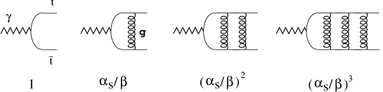
Figure 1: The ladder diagrams for the process $\gamma^{*}\to t\bar{t}$. The diagram where $n$ uncrossed gluons are exchanged has the behavior $(\alpha_{s}/\beta)^{n}$ near threshold.

Hence, the contribution of the ${\cal O}(\alpha_{s}^{n})$ ladder diagram will not be small even for a large $n$ if $\beta\hbox{ \raise 3.0pt\hbox to0.0pt{$<$}\raise-3.0pt\hbox{$\sim$} }\alpha_{s}$. These $(\alpha_{s}/\beta)^{n}$ singularities which appear at this specific kinematical configuration are known as “threshold singularities” or “Coulomb singularities”.

Intuitively the appearance of $(\alpha_{s}/\beta)^{n}$ can be interpreted as follows. When the produced $t$ and $\bar{t}$ have small velocities ($\beta\hbox{ \raise 3.0pt\hbox to0.0pt{$<$}\raise-3.0pt\hbox{$\sim$} }\alpha_{s}$), they are trapped by the attractive force mediated by the exchange of gluons. Thus, they stay close to each other for a long time and multiple exchanges of gluons (higher order ladder diagrams) become more significant and the strong interaction is enhanced accordingly.

Since the higher order terms remain unsuppressed in the threshold region, we are led to resum these contributions. The resummation technique is known since long time. The leading $(\alpha_{s}/\beta)^{n}$ terms can be incorporated in the $t\bar{t}$ pair production vertex as

$$\Gamma^{\mu}=-\,\gamma^{\mu}\,(E-{\bf p}_{t}^{2}/m_{t}+i\Gamma_{t})\,\tilde{G}({\bf p}_{t};E),$$ (4)

where $E=\sqrt{s}-2m_{t}$ is the energy measured from the threshold. $\tilde{G}({\bf p};E)$ is the momentum-space Green function of the non-relativistic Schrödinger equation with the Coulomb potential:

$$\left[\left(-\,\frac{\nabla^{2}}{m_{t}}+V(r)\right)-(E+i\Gamma_{t})\right]G({\bf x};E)=\delta^{3}({\bf x}),$$ (5)

$$~{}~{}~{}\tilde{G}({\bf p};E)=\int d^{3}{\bf x}\,e^{-i{\bf p}\cdot{\bf x}}\,G({\bf x};E),$$ (6)

$$~{}~{}~{}~{}~{}~{}V(r)=-\,C_{F}\,\frac{\alpha_{s}}{r},$$ (7)

where $C_{F}=4/3$ is the color factor.

It is possible to perform a systematic perturbative expansion of the cross sections in the threshold region. Roughly speaking, one may identify

$$\begin{array}[]{llc}{\displaystyle\sum_{~{}}c_{n}^{(0)}(\alpha_{s}^{n}/\beta^{n})}&:&\mbox{leading}\\ {\displaystyle\sum_{~{}}c_{n}^{(1)}(\alpha_{s}^{n+1}/\beta^{n})}&:&{\cal O}(\alpha_{s})~{}\mbox{correction}\\ {\displaystyle\sum_{~{}}c_{n}^{(2)}(\alpha_{s}^{n+2}/\beta^{n})}&:&{\cal O}(\alpha_{s}^{2})~{}\mbox{correction}\\ ~{}~{}~{}~{}~{}~{}~{}\vdots&&\vdots\end{array}$$ (12)

For all interesting physical quantities (cross sections) for $e^{+}e^{-}\to t\bar{t}$ near threshold, calculations of the full ${\cal O}(\alpha_{s})$ corrections have been completed so far [14, 25]. Meanwhile calculations of the second order corrections are currently in progress.

One typical example of the ${\cal O}(\alpha_{s})$ corrections is the radiative corrections to the Coulomb-gluon-exchange kernel, whose net effect is to replace the fixed coupling constant in the Coulomb potential in Eq. (7) by the running coupling constant, $\alpha_{s}\to\alpha_{s}(\mu\simeq 1/r)$. We thus have the QCD potential which becomes weaker than the Coulomb potential at short distances.

Recently, there has been considerable progress in the theoretical calculations of the higher order corrections to the Coulomb bound-state problems. New contributions have been calculated analytically for QED bound-states [32, 33], which could not be achieved using the conventional bound-state approaches. The corrections that originate from the relativistic regime and those from the non-relativistic regime have been separated using an effective Lagrangian formalism [34]. The real difficult part of the calculations is now reduced to the ordinary second-order (relativistic) perturbative calculation of the cross section, which requires no knowledge of the bound-state problems. The readers are referred to e.g. Refs. [35, 36] for introduction to the formalism.

2 Production of Top Quark

To understand the physics concerning the production of top quarks, one needs to keep in mind that the $t\bar{t}$ production vertex is proportional to the Green function of the non-relativistic Schrödinger equation:

$$\Gamma^{\mu}\propto\tilde{G}({\bf p}_{t};E)=-\sum_{n}\frac{\phi_{n}({\bf{p}}_{t})\psi_{n}^{*}({\bf{0}})}{E-E_{n}+i\Gamma_{t}},$$ (13)

where

$$\left[\frac{\hat{{\bf{p}}}^{2}}{m_{t}}+V_{\rm QCD}(r)\right]\left|\,{n}\,\right>=E_{n}\left|\,{n}\,\right>,~{}~{}~{}\begin{array}[]{l}\phi_{n}({\bf{p}})=\hbox{$\left<{{\bf{p}}}\,\vrule\,{n}\right>$}\rule[-8.53581pt]{0.0pt}{22.76219pt}\\ \psi_{n}({\bf{x}})=\hbox{$\left<{{\bf{x}}}\,\vrule\,{n}\right>$}\end{array}$$ (16)

defines the wave functions of the energy eigenstate of the QCD potential.

2.1 Total Cross Section

The first observable we measure in the $t\bar{t}$ threshold region will be the total cross section. Via the optical theorem, the total cross section can be written as [2, 6]

$$\sigma_{\rm tot}(e^{+}e^{-}\to t\bar{t})\propto-{\rm Im}\sum_{n}\frac{|\psi_{n}({\bf{0}})|^{2}}{E-E_{n}+i\Gamma_{t}}.$$ (17)

One sees that the energy dependence of the total cross section is determined by the resonance spectra. Due to the large width $\Gamma_{t}$ of the top quark, however, distinct resonance peaks are smeared out. The resonances merge with one another, leading to a broad enhancement of the cross section over the threshold region as seen in Fig. 2.

Figure 2: The total cross section vs. energy, $E=\sqrt{s}-2m_{t}$. The solid curve is calculated from the Green function. The dashed curve shows the tree-level total cross section for a stable top quark.

(We will show explicitly the resonance spectra below.) In the same figure, the tree level cross section is also shown as a dashed curve. Despite the disappearance of each resonance peak, one sees that the cross section is indeed largely enhanced by the QCD interaction, and that inclusion of the QCD binding effect is mandatory for a proper account of the cross section in the threshold region.

2.2 Top Momentum Distribution

Next we consider the top-quark momentum ($|{\bf{p}}_{t}|$) distribution near $t\bar{t}$ threshold [8, 9]. It has been shown that experimentally it will be possible to reconstruct the top-quark momentum ${\bf{p}}_{t}$ from its decay products with reasonable resolution and detection efficiency. Fig. 3(a) shows a comparison of reconstructed top momenta (solid circles) with that of generated ones (histogram), where the events are generated by a Monte Carlo generator and are reconstructed after going through detector simulators and selection cuts [17]. The figure demonstrates that the agreement is fairly good.

Theoretically, the top-quark momentum distribution is given by

$$\frac{d\sigma}{d|{\bf{p}}_{t}|} \propto \biggl{|}\sum_{n}\frac{\phi_{n}({\bf{p}}_{t})\psi_{n}^{*}({\bf{0}})}{E-E_{n}+i\Gamma_{t}}\biggl{|}^{2}+\mbox{(sub-leading)}.$$ (18)

The $|{\bf{p}}_{t}|$-distribution is thus governed by the momentum-space wave functions of the resonances. By measuring the momentum distribution, essentially we measure (a superposition of) the wave functions of the toponium resonances. Shown in Fig. 3(b) are the top momentum distributions for various energies.

     

Figure 3: (a) Reconstructed momentum distribution (solid circles) for the lepton-plus-4-jet mode, compared with the generated distribution (histogram). The Monte Carlo events were generated with $\alpha_{s}(M_{Z})=0.12$ and $m_{t}=150$ GeV [17]. (b) Top-quark momentum distributions $d\sigma/d|{\bf{p}}_{t}|$ for various c.m. energies measured from the lowest lying resonance, $\Delta E=\sqrt{s}-M_{1S}$, taking $\alpha_{s}(M_{Z})=0.118$ and $m_{t}=175$ GeV.

One may also vary the magnitude of $\alpha_{s}$ and confirm that the distribution is indeed sensitive to the resonance wave functions [8, 9]. Hence, the momentum distribution provides information independent of that from the total cross section.

Note that the toponium states will be the first quarkonium resonances whose wave functions can be measured experimentally. For comparison, consider $\Upsilon(4S)$, which decays into $B$ and $\bar{B}$. Since the mass of $B$($\bar{B}$) is fixed, its momentum is fixed by the on-shell condition; the momentum distribution of $B$($\bar{B}$) is a $\delta$-function in this case. Meanwhile, in the case of toponium, the invariant mass distribution of top quarks has a large width, and accordingly the top-quark three momenta have a distribution that is just sufficiently broad for probing the wave functions of the resonances.

2.3 Forward-Backward Asymmetry

Another observable that can be measured experimentally is the forward-backward asymmetry of the top quark [10]. Generally in a fermion pair production process, a forward-backward asymmetric distribution originates from an interference of the vector and axial-vector $f\bar{f}$ production vertices at tree level of electroweak interaction. One can show from the spin-parity argument that in the threshold region the $t\bar{t}$ vector vertex creates S-wave resonance states, while the $t\bar{t}Z$ axial-vector vertex creates P-wave states. Therefore, by observing the forward-backward asymmetry of the top quark, we observe an interference of the S-wave and P-wave states.

In general, S-wave resonance states and P-wave resonance states have different energy spectra. So if the c.m. energy is fixed at either of the spectra, there would be no contribution from the other. However, the widths of resonances are large for the toponium in comparison to their level splittings, which permit sizable interferences of the S-wave and P-wave states. Fig. 4 shows the pole position $E_{n}\!-\!i\Gamma_{t}$ of these states on the complex energy plane.

Figure 4: The positions of poles of the S-wave and P-wave states on the complex energy plane, together with the forward-backward asymmetry as a function of the energy, taking $\alpha_{s}(M_{Z})=0.118$ and $m_{t}=175$ GeV. The right-axis is for the forward-backward asymmetry.

One sees that the widths of the resonances are comparable to the mass difference between the lowest lying S-wave and P-wave states, and exceeds by far the level spacings between higher S-wave and P-wave states. This gives rise to a forward-backward asymmetry even below threshold, and provides information on the resonance level structure which is concealed in the total cross section. Shown on the same figure is the forward-backward asymmetry as a function of the energy. It is seen that the asymmetry takes its minimum value at around the lowest lying S-wave state, where the interference is smallest, and increases up to $\sim 10$% with energy as the resonance spectra appear closer to each other. One may also confirm that essentially the forward-backward asymmetry measures the degree of overlap of the S-wave and P-wave states by varying the coupling constant $\alpha_{s}$ or the top quark decay width $\Gamma_{t}$.

The resonance level structure is determined by QCD, whereas the resonance widths are determined by electroweak interaction. The interplay of the two interactions generates the forward-backward asymmetry.

3 Decay of Top Quark and Final-State Interactions

Now we turn to decay processes of the top quark near threshold. The top quarks produced via $e^{+}e^{-}\to t\bar{t}$ in the threshold region will be highly polarized [29]. Even for an unpolarized $e^{-}$ beam, the top quarks have a natural polarization of around 40%, while for a longitudinally polarized $e^{-}$ beam (an obvious option for NLC) the polarization of top quarks can be raised close to 100% [21, 24]. Therefore, in principle, the threshold region can be an ideal place for studying the top quark decay processes using the highly polarized top quark samples and the largest $t\bar{t}$ production cross section.

3.1 Free Polarized Top Quark Decay

Detailed studies of the decay of free polarized top quarks have already been available including the full ${\cal O}(\alpha_{s})$ corrections [37, 20, 38]. A nice example is that of the energy-angular distribution of charged leptons $l^{+}$ in the semi-leptonic decay of the top quark. In leading order, the $l^{+}$ distribution has a form where the energy and angular dependences are factorized [39, 40]:

$$\frac{d\Gamma_{t\to bl^{+}\nu}({\bf{S}})}{dE_{l}d\Omega_{l}}=h(E_{l})\,(1+|{\bf{S}}|\cos\theta_{l})\,+\,({\cal O}(\alpha_{s})~{}\mbox{correction}).$$ (19)

Here $E_{l}$, $\Omega_{l}$, and $\theta_{l}$ denote, respectively, the $l^{+}$ energy, the solid angle of $l^{+}$, and the angle between the $l^{+}$ direction and the top polarization vector ${\bf{S}}$, all of which are defined in the top-quark rest frame. Hence, we may measure the top-quark polarization with maximal sensitivity using the $l^{+}$ angular distribution.

3.2 Effects of Final-State Interactions

Close to threshold, the above precise analyses of the free top-quark decays do not apply directly because of the existence of corrections unique to this region. Namely, these are the final-state interactions due to gluon exchange between $t$ and $\bar{b}$ ($\bar{t}$ and $b$) or between $b$ and $\bar{b}$. (Fig. 5)

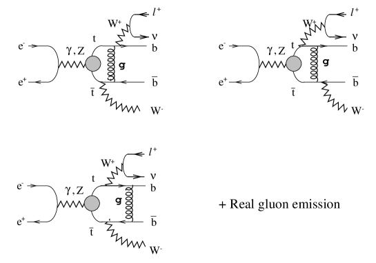
Figure 5: Diagrams for the final-state interactions for $e^{+}e^{-}\to t\bar{t}\to bl^{+}\nu\bar{b}W^{-}$.

The size of the corrections is at the 10% level in the threshold region, hence it is necessary to incorporate their effects in precision studies of top-quark production and decay near threshold.

Before presenting the formula for these final-state interaction corrections, let us first see what kind of effects we expect from physics ground [25].

$\bullet$ Top Momentum Distribution

Perhaps it is easiest to understand the effect of final-state interactions on the top momentum distribution. Fig. 6(a) shows the momentum distribution with (solid) and without (dashed) the final-state interactions.

Figure 6: (a) The top momentum distribution with (solid) and without (dashed) the final-state interaction corrections for $\alpha_{s}(M_{Z})=0.118$ and $m_{t}=175$ GeV. (b) Attractive force between $\bar{t}$ and $b$ (from $t$ decay). The momentum transfer $\delta{\bf{p}}_{b}=-\delta{\bf{p}}_{\bar{t}}$ due to the attraction is indicated by thick arrows.

We see that the average momentum is reduced due to the interaction. To understand this, consider for example the case where $t$ decays first. Fig. 6(b) shows the attractive force between $\bar{t}$ and $b$, which deflects the trajectory of $b$. Since ${\bf{p}}_{t}$ is reconstructed from the $bW^{+}$ momenta at time $\tau\to\infty$, it is obvious that the reconstructed momentum $|{\bf{p}}_{t}|=|{\bf{p}}_{b}+{\bf{p}}_{W^{+}}|$ is decreased by the attraction.

$\bullet$ Forward-Backward Asymmetric Distribution

Next we consider the $\cos\theta_{te}$ distribution of the top quark. ($\theta_{te}$ denotes the angle between $t$ and $e^{-}$ in the $t\bar{t}$ c.m. frame.) We consider the case where $\bar{t}$ decays first and examine the interaction between $t$ and $\bar{b}$. The $t$ and $\bar{t}$ pair-produced near threshold in $e^{+}e^{-}$ collisions have their spins approximately parallel or anti-parallel to the $e^{-}$ beam direction ($\hat{{\bf{n}}}_{\|}$) and the spins are always oriented parallel to each other. On the other hand, the decay of $\bar{t}$ occurs via a $V\!-\!A$ coupling, and $\bar{b}$ is emitted preferably in the spin direction of the parent $\bar{t}$, see Fig. 7.

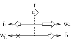
Figure 7: Typical configurations in the decay of $\bar{t}$ with definite spin orientation. Transverse $W^{-}$ ($W^{-}_{T}$) tends to be emitted in the direction of the $\bar{t}$ spin orientation, while longitudinal $W^{-}$ ($W^{-}_{L}$) is emitted in the opposite direction due to helicity conservation. For $m_{t}\simeq 175$ GeV, $\bar{t}$ decays mainly to $W^{-}_{L}$, hence $\bar{b}$ is emitted more in the $\bar{t}$ spin direction.

More precisely, the excess of the $\bar{b}$’s emitted in the $\bar{t}$ spin direction over those emitted in the opposite direction is given by $\kappa=(m_{t}^{2}-2M_{W}^{2})/(m_{t}^{2}+2M_{W}^{2})$. Now suppose $t$ and $\bar{t}$ have their spins in the $\hat{{\bf{n}}}_{\|}$ direction. Then $\bar{b}$ will be emitted dominantly in the $\hat{{\bf{n}}}_{\|}$ direction. One can see from Fig. 8(a) that in this case $t$ is always attracted to the forward direction due to the attractive force between $t$ and $\bar{b}$.

Figure 8: Attractive force between $t$ and $\bar{b}$ when the $t$ and $\bar{t}$ spins are oriented in the (a) $\hat{{\bf{n}}}_{\|}$ direction, and in the (b) $-\hat{{\bf{n}}}_{\|}$ direction. The momentum transfer $\delta{\bf{p}}_{b}=-\delta{\bf{p}}_{\bar{t}}$ due to the attraction is indicated by thick black arrows.

The direction of the attractive force will be opposite if $t$ and $\bar{t}$ have their spins in the $-\hat{{\bf{n}}}_{\|}$ direction (Fig. 8(b)). Thus, polarized top quarks will be pulled in a definite (forward or backward) direction, and we may expect that a forward-backward asymmetric distribution of the top quark $\sim\kappa\,S_{\|}\cos\theta_{te}$ is generated by the final-state interaction. ($S_{\|}$ denotes the $\hat{{\bf{n}}}_{\|}$-component of the top polarization vector ${\bf{S}}$.)

$\bullet$ Top-Quark Polarization Vector

From Fig. 8 we can also learn the effect of the final-state interaction on the top polarization vector. We have seen that if the $t$ and $\bar{t}$ spins are oriented in the $\hat{{\bf{n}}}_{\|}$ direction, $t$ will be attracted to the forward direction due to the attraction by $\bar{b}$, and oppositely attracted to the backward direction if the $t$ and $\bar{t}$ spins are in the $-\hat{{\bf{n}}}_{\|}$ direction. This means that in the forward region ($\cos\theta_{te}\simeq 1$) the number of $t$’s with spin in $\hat{{\bf{n}}}_{\|}$ direction increases, whereas in the backward region the number of those with spin in the opposite direction increases. Or equivalently, the $\hat{{\bf{n}}}_{\|}$-component of the top-quark polarization vector increases in the forward region and decreases in the backward region. We may thus conjecture that the top-quark polarization vector is modified as $\delta S_{\|}\sim\kappa\cos\theta_{te}$ due to the interaction between $t$ and $\bar{b}$.

$\bullet$ $l^{+}$ Energy-Angular Distribution

Finally let us examine the effect of the attraction between $b$ and $\bar{t}$ on the $l^{+}$ energy-angular distribution in the semi-leptonic decay of $t$. The $b$-quark from $t$ decay will be attracted in the direction of $\bar{t}$ due to the gluon exchange between these two particles. We show schematically typical configurations of the particles in the top-quark semileptonic decay in Fig. 9.

Figure 9: Typical configurations of the particles in semileptonic decay of $t$ when the $b$-quark is emitted in the $\bar{t}$ direction. Due to the boost by $W^{+}$, there will be an energy-angle correlation of $l^{+}$.

It can be seen that if the probability for $b$ being emitted in the $\bar{t}$ direction increases, correspondingly the probability for particular $l^{+}$ energy-angular configurations increases. These configurations are either “$E_{l}$ is small and $l^{+}$ emitted in $-{\bf{p}}_{t}$ direction” or “$E_{l}$ is large and $l^{+}$ emitted in ${\bf{p}}_{t}$ direction”.

3.3 Lepton Energy-Angular Distribution Near $t\bar{t}$ Threshold

Here, we present the formula for the charged lepton energy-angular distribution in the decay of top quarks that are produced via $e^{+}e^{-}\to t\bar{t}$ near threshold.

First, without including the final-state interactions, the differential distribution of $t$ and $l^{+}$ has a form where the production and decay processes of the top quark are factorized [41]:

$$\frac{d\sigma(e^{+}e^{-}\!\to t\bar{t}\to bl^{+}\nu\bar{b}W^{-})}{d^{3}{\bf{p}}_{t}dE_{l}d\Omega_{l}}=\frac{d\sigma(e^{+}e^{-}\!\to t\bar{t})}{d^{3}{\bf{p}}_{t}}\times\frac{1}{\Gamma_{t}}\,\frac{d\Gamma_{t\to bl^{+}\nu}({\bf{S}})}{dE_{l}d\Omega_{l}}.$$ (20)

Namely, the cross section is given as a product of the production cross section of unpolarized top quarks and the differential decay distribution of $l^{+}$ from polarized top quarks. The above formula holds true even including all ${\cal O}(\alpha_{s})$ corrections other than the final-state interactions.

Including the final-state interactions, the factorization of production and decay processes is destroyed. The formula including the full ${\cal O}(\alpha_{s})$ corrections is given by [25]

$$\frac{d\sigma(e^{+}e^{-}\!\to t\bar{t}\to bl^{+}\nu\bar{b}W^{-})}{d^{3}{\bf{p}}_{t}dE_{l}d\Omega_{l}}=\frac{d\sigma(e^{+}e^{-}\!\to t\bar{t})}{d^{3}{\bf{p}}_{t}}\times(1+\delta_{0}+\delta_{1}\cos\theta_{te})$$

$$\times\frac{1}{\Gamma_{t}}\,\frac{d\Gamma_{t\to bl^{+}\nu}({\bf{S}}+\delta{\bf{S}})}{dE_{l}d\Omega_{l}}\times\left[1+\xi(|{\bf{p}}_{t}|,E,E_{l},\cos\theta_{lt})\right].$$

(21)

Here, the first line on the right-hand-side shows that there are corrections to the top-quark production cross section, while the second line shows that the correction to the decay distribution of $l^{+}$ is accounted for by a modification of the parent top-quark polarization vector, and finally there is a non-factorizable correction $\xi$ which cannot be assigned either to the production or the decay process alone.

We have already seen in Fig. 6(a) that the top momentum distribution is modified by $\delta_{0}$ to take a lower average momentum. The forward-backward asymmetric distribution and the top polarization vector get corrections as

$$\delta_{1}\cos\theta_{te}=\kappa S_{\|}\cos\theta_{te}\times\frac{1}{2}\psi_{\rm{}_{R}},$$ (22)

$$\delta{\bf{S}}=\left[1-(S_{\|})^{2}\right]\times\kappa\cos\theta_{te}\times{\frac{1}{2}}\psi_{\rm{}_{R}}\cdot\hat{{\bf{n}}}_{\|}$$ (23)

with

$$\psi_{\rm{}_{R}}(|{\bf{p}}_{t}|,E)=-\,C_{F}\!\cdot\!4\pi\alpha_{s}\,\mbox{Pr.}\int\mbox{$\frac{d^{3}{\bf{q}}}{(2\pi)^{3}}$}\,\,\frac{1\,}{|{\bf{q}}\!-\!{\bf{p}}_{t}|^{3}}\,\frac{{\bf{p}}_{t}\!\cdot\!({\bf{q}}\!-\!{\bf{p}}_{t})}{|{\bf{p}}_{t}|\,|{\bf{q}}\!-\!{\bf{p}}_{t}|}\,2\,\mbox{Re}\biggl{[}\frac{\tilde{G}({\bf{q}};E)}{\tilde{G}({\bf{p}}_{t};E)}\biggl{]}.$$

The above formulas (22) and (23) have exactly the forms that we anticipated in the previous subsection if $\psi_{\rm{}_{R}}$ is positive. Indeed, the numerical evaluation in Ref. [24] shows that $\psi_{\rm{}_{R}}(|{\bf{p}}_{t}|,E)\hbox{ \raise 3.0pt\hbox to0.0pt{$>$}\raise-3.0pt\hbox{$\sim$} }0$ holds in the entire threshold region.

We show the $\cos\theta_{lt}$ and $E_{l}$ dependences of the non-factorizable correction $\xi$ as a 3-dimensional plot in Fig. 10.

Figure 10: A three-dimensional plot of $\xi$ as a function of $2E_{l}/m_{t}$ ($x$-axis) and $\cos\theta_{te}$ ($y$-axis).

One can see that $\xi$ takes comparatively large positive values for either “small $E_{l}$ and $\cos\theta_{lt}\simeq-1$” or “large $E_{l}$ and $\cos\theta_{lt}\simeq+1$”. Oppositely, in the other two corners of the $E_{l}$–$\cos\theta_{lt}$ plane $\xi$ becomes negative. These features are consistent with our previous qualitative argument. The typical magnitude of $\xi$ is 10–20%.

Thus, the theoretical prediction for the distribution of $l^{+}$ from the top decay is under good control in the $t\bar{t}$ threshold region, together with a good qualitative understanding.

Prior to the calculation of the $l^{+}$ differential distribution Eq. (21), an inclusive quantity, the mean value $\langle n\ell\rangle$ of the charged lepton four-momentum projection on an arbitrarily chosen four-vector $n$, was proposed as an observable sensitive to the top quark polarization, and this quantity was calculated including the final-state interactions [24].

3.4 Observable Proper to the Decay Process

We have seen that the final-state interactions destroy the factorization of the production and decay cross sections of the top quark. In order to study the decay of the top quark in a clean environment in the threshold region, it would be useful if we could find an observable which depends only on the decay process of free polarized top quarks, $d\Gamma_{t\to bl^{+}\nu}({\bf{S}})/dE_{l}d\Omega_{l}$. In fact, such an observable can be constructed, which at the same time preserves most of the differential information of the $l^{+}$ energy-angular distribution.

It is possible to show (with sufficient reasoning) that the non-factorizable correction factor $\xi(|{\bf{p}}_{t}|,E,E_{l},\cos\theta_{lt})$ is invariant under a transformation of the $l^{+}$ kinematical variables

$$E_{l} \to E^{\prime}_{l}=2m_{t}\left(\frac{m_{t}^{2}+M_{W}^{2}}{M_{W}^{2}}-\frac{2m_{t}}{E_{l}}\right)^{-1},$$ (25)

$${\bf{p}}_{l} \to {\bf{p}}_{l}^{\prime}~{}~{}~{}~{}\mbox{such that}~{}~{}~{}\cos\theta_{lt}\to-\cos\theta_{lt}.$$ (26)

Using this symmetry, it is possible to cancel out not only the non-factorizable correction but also the top production cross section by taking an appropriate ratio of cross sections.

Let us define an observable as

$$\overline{A}(E_{l},a\!=\!{\bf{S}}\!\cdot\!{\bf{p}}_{l})$$

$$\equiv\frac{\displaystyle\int{d^{3}{\bf{p}}_{t}d\Omega_{l}}\,\,\delta\!\left({\bf{S}}\!\cdot\!{\bf{p}}_{l}-a\right)\left[\frac{d\sigma(e^{+}e^{-}\!\to t\bar{t}\to bl^{+}\nu\bar{b}W^{-})}{d^{3}{\bf{p}}_{t}dE_{l}d\Omega_{l}}\right]_{E_{l},{\bf{p}}_{l}}}{\displaystyle\int{d^{3}{\bf{p}}_{t}d\Omega_{l}}\,\,\delta\!\left({\bf{S}}\!\cdot\!{\bf{p}}_{l}+a\right)\left[\frac{d\sigma(e^{+}e^{-}\!\to t\bar{t}\to bl^{+}\nu\bar{b}W^{-})}{d^{3}{\bf{p}}_{t}dE_{l}d\Omega_{l}}\right]_{E^{\prime}_{l},{\bf{p}}_{l}}}.$$ (27)

Here, the top-quark polarization vector ${\bf{S}}$ in the delta functions depends on ${\bf{p}}_{t}$ [25]. The numerator and denominator, respectively, depend on two external kinematical variables (the lepton energy and the lepton angle from the parent top-quark polarization vector), and all other variables are integrated out before taking the ratio.

Then substituting the differential distribution Eq. (21), one can show that theoretically $\overline{A}$ is determined solely from the decay distribution of free polarized top quarks:

$$\overline{A}(E_{l},a)=\left[\frac{d\Gamma_{t\to bl^{+}\nu}({\bf{S}})}{dE_{l}d\Omega_{l}}\right]_{E_{l},{\bf{S}}\cdot{\bf{p}}_{l}=a}\biggl{/}\left[\frac{d\Gamma_{t\to bl^{+}\nu}({\bf{S}})}{dE_{l}d\Omega_{l}}\right]_{E_{l}^{\prime},{\bf{S}}\cdot{\bf{p}}_{l}=-a}.$$ (28)

This is a general formula that is valid even if the decay vertices of the top quark deviate from the standard-model forms.

This quantity will be useful from the theoretical point of view. If one claims that he calculates $\overline{A}(E_{l},a)$ defined in Eq. (27) in the threshold region, it can be calculated without including any bound-state effects or final-state interaction corrections but only from a decay distribution of free polarized top quarks via Eq. (28).

4 Summary

We have reviewed the physics concerning the production and decay of top quarks in the $t\bar{t}$ threshold region.

Theoretical predictions of cross sections near $t\bar{t}$ threshold are well under control. The full ${\cal O}(\alpha_{s})$ corrections as well as part of the second order corrections are already available.

As for the top-quark production process, there are three independent observables that are unique to the $t\bar{t}$ threshold region. The total cross section is enhanced by the QCD interaction, but distinct resonance peaks are smeared out due to the large decay widths of the resonances. The top quark momentum measurement will probe the resonance wave functions. The top-quark forward-backward asymmetry measures the overlaps of the S and P-wave resonance states.

Studies of the decay of top quarks in the $t\bar{t}$ threshold region have just been started. First, an inclusive observable $\langle n\ell\rangle$ was calculated, which is sensitive to the top polarization. Recently, the differential decay distribution of $l^{+}$ in the top-quark semileptonic decay has been calculated. The final-state interactions modify the top-quark production cross section, the top-quark polarization vector, and also gives rise to a non-factorizable correction at the level of 10–20%.

We defined a new observable $\overline{A}(E_{l},a)$ in the threshold region, which depends only on the decay process of free polarized top quarks. This quantity can be calculated (including e.g. anomalous top-quark decay vertices) without any knowledge of the bound-state effects or the final-state interactions, but assuming the highly polarized top quark samples expected in the $t\bar{t}$ threshold region. Further studies in this direction are demanded.

Finally, a supplementary remark would be in order for those who are interested to know how accurately various physical parameters ($m_{t}$, $\alpha_{s}$, $\Gamma_{t}$, $M_{H}$, $g_{tH}$, etc.) can be measured in the $t\bar{t}$ threshold region at NLC. The results from quantitative studies taking into account realistic experimental conditions can be found in Refs. [17, 19, 23] for $m_{t}=150$ GeV, 170 GeV and 180 GeV, respectively.

The first half of the paper is based on the studies in collaboration with K. Fujii, K. Hagiwara, K. Hikasa, S. Ishihara, T. Matsui, H. Murayama and C.-K. Ng. The latter half is based on our recent work with M. Peter. The author wishes to thank all of them. The author is also grateful to A. Hoang, M. Jeżabek and J. Kühn for fruitful discussion. The author is thankful to K. Melnikov, M. Peter and S. Recksiegel for comments on the manuscript. This work is supported by the Alexander von Humboldt Foundation.

References

- [1] For reviews on physics that can be covered at NLC, see Proceedings of Workshop on Physics and Experiments with Linear Colliders, Saariselka, Finland, 1991, edited by R. Orava, P. Elrola and M. Nordbey (World Scientific, Singapore, 1992); JLC Group, KEK Report 92-16 (1992); W. Bernreuther, et al., in Collisions at 500 GeV: The Physics Potential, Part A, B, C and D, DESY 92-123, (1992), DESY 93-123, (1993), DESY 96-123, (1996); Proceedings of the Workshop on Physics and Experiments with Linear Colliders (Waikoloa, Hawaii, April 1993); K. Fujii, Talk given at 22nd INS International Symposium on Physics with High Energy Colliders, KEK preprint, 94-38 (1994).
- [2] V.S. Fadin and V.A. Khoze, JETP Lett. 46, 525 (1987); Sov. J. Nucl. Phys. 48, 309 (1988).
- [3] S. Komamiya, in Research Directions for the Decade, Proceedings of the 1990 Summer Study on High Energy Physics, Snowmass, Colorado, 1990, edited by E. Berger (World Scientific, Singapre, 1992), p.459.
- [4] V. Fadin and Yakovlev, Sov. J. Nucl. Phys. 53, 688 (1991).
- [5] W. Kwong, Phys. Rev. D43, 1488 (1991).
- [6] M. Strassler and M. Peskin, Phys. Rev. D43, 1500 (1991).
- [7] M. Peskin, in Proceedings of Workshop on Physics and Experiments with Linear Colliders, Saariselka, Finland, 1991, edited by R. Orava, P. Elrola and M. Nordbey (World Scientific, Singapore, 1992).
- [8] Y. Sumino, K. Fujii, K. Hagiwara, H. Murayama, and C.-K. Ng, Phys. Rev. D47, 56 (1993).
- [9] M. Jeżabek, J.H. Kühn and T. Teubner, Z. Phys. C 56 (1992) 653; M. Jeżabek and T. Teubner, Z. Phys. C 59 (1993) 669.
- [10] H. Murayama and Y. Sumino, Phys. Rev. D47, 82 (1993).
- [11] P. Igo-Kemenes, M. Martinez, R. Miquel, and S. Orteu, Talk given at the Workshop on Physics and Experiments with Linear Colliders (Waikoloa, Hawaii, April 1993).
- [12] J.H. Kühn, in: F.A. Harris et al. (eds.), Physics and Experiments with Linear Colliders, Singapore: World Scientific, 1993, p.72.
- [13] K. Melnikov and O. Yakovlev, Phys. Lett. B324, 217 (1994).
- [14] Y. Sumino, Ph.D. Thesis, University of Tokyo preprint, UT-655 (1993).
- [15] V. Fadin, V. Khoze, and A. Martin, Phys. Rev. D49, 2247 (1994); Phys. Lett. B320, 141 (1994).
- [16] V. Khoze and W. Sjöstrand, Phys. Lett. B328, 466 (1994).
- [17] K. Fujii, T. Matsui and Y. Sumino, Phys. Rev. D50, 4341 (1994).
- [18] W. Mödritsch and W. Kummer, Nucl. Phys. B430, 3 (1994); W. Kummer and W. Mödritsch, Z. Phys. C66, 225 (1995).
- [19] Y. Sumino, Acta Phys. Polonica B25 1837 (1994).
- [20] M. Jeżabek, Nucl. Phys. 37 B (Proc.Suppl.) (1994) 197.
- [21] R. Harlander, M. Jeżabek, J.H. Kühn and T. Teubner, Phys. Lett. B 346 (1995) 137.
- [22] W. Mödritsch, Nucl. Phys. B475, 507 (1996).
- [23] P. Comas, R. Miquel, M. Martinez and S. Orteu, in edited by P. Zerwas, Collisions at TeV Energies: The Physics Potential, Part D, DESY 96-123D, (1996).
- [24] R. Harlander, M. Jeżabek, J. Kühn, and M. Peter, Z. Phys. C73, 477 (1997).
- [25] M. Peter and Y. Sumino, hep-ph/9708223.
- [26] CDF Collaboration, Fermilab preprint, FERMILAB-PUB-97-284-E (1997).
- [27] D0 Collaboration, Phys. Rev. Lett. 79, 1197 (1997).
- [28] M. Jeżabek and J.H. Kühn, Phys. Rev. D 48 (1993) R1910; erratum Phys. Rev. D 49 (1994) 4970; and references therein.
- [29] J.H. Kühn, Acta Phys. Polonica B 12 (1981) 347.
- [30] J.H. Kühn and P.M. Zerwas, Phys. Rep. 167, 321 (1988).
- [31] K. Hagiwara, K. Kato, A. D. Martin and C.-K. Ng, Nucl. Phys. B344, 1 (1990).
- [32] A. Hoang, hep-ph/9704325.
- [33] A. Hoang, P. Labelle and S. Zebarjad, hep-ph/9707337.
- [34] W. Caswell and G. Lepage, Phys. Rev. A20, 36 (1979).
- [35] P. Labelle, hep-ph/9608491; P Labelle and S. Zebarjad, hep-ph/9611313.
- [36] B. Grinstein and I. Rothstein, hep-ph/9703298.
-
[37]
A. Czarnecki, M. Jeżabek and J.H. Kühn,
Nucl. Phys. B 351 (1991) 70;
A. Czarnecki and M. Jeżabek, Nucl. Phys. B 427 (1994) 3. - [38] M. Jeżabek, Acta Phys. Polonica B 26 (1995) 789.
- [39] J.H. Kühn and K.H. Streng, Nucl. Phys. B 198 (1982) 71.
- [40] M. Jeżabek and J.H. Kühn, Nucl. Phys. B 320 (1989) 20.
- [41] See, for example, the talk given by B. Grzadkowski in these proceedings.