TUM/T39-97-28

Hard Exclusive Meson Production
and
Nonforward Parton Distributions

L. Mankiewicz, G. Piller and T. Weigl

Physik Department, Technische Universität München,
D-85747 Garching, Germany

Abstract

We present an analysis of twist-$2$, leading order QCD amplitudes for hard exclusive leptoproduction of mesons in terms of double/nonforward parton distribution functions. After reviewing some general features of nonforward nucleon matrix elements of twist-$2$ QCD string operators, we propose a phenomenological model for quark and gluon nonforward distribution functions. The corresponding QCD evolution equations are solved in the leading logarithmic approximation for flavor nonsinglet distributions. We derive explicit expressions for hard exclusive $\pi^{0}$, $\eta$, and neutral vector meson production amplitudes and discuss general features of the corresponding cross sections.

1 Introduction

Our current knowledge of the sub-structure of nucleons is based to a large extent on high-energy scattering experiments which probe its quark and gluon distribution functions. The most prominent processes in this respect are deep-inelastic scattering and Drell-Yan leptoproduction. In addition a large amount of information can be deduced from measurements of electromagnetic and weak form factors.

Recently new observables, namely nonforward parton distribution functions, attract a great amount of interest. Although being discussed already some time ago [1, 2, 3], they were introduced in the context of the spin structure of nucleons recently in Ref.[4]. Nonforward parton distributions are a generalization of ordinary parton distributions [4, 5]. However they are also closely related to nucleon form factors. Thus they combine different aspects of the nucleon structure and offer new insights.

To summarize the relation of nonforward parton distributions to ordinary parton distributions recall that at the twist-$2$ level the latter can be represented as normalized Fourier transforms of forward nucleon matrix elements of non-local QCD operators [6], constructed as gauge-invariant overlap of two quark or gluon fields separated by a light-like distance. Nonforward parton distributions are defined by the same non-local QCD operators – just sandwiched between nucleon states with different momenta and eventually spin. Equally close is the relation to nucleon form factors which are defined by nonforward matrix elements of the same QCD operators taken in the local limit.

Nonforward parton distributions are probed in processes where the nucleon target recoils elastically. To select twist-$2$ correlations a large scale has to be involved. One possible process is deeply-virtual Compton scattering as investigated in Ref.[4]. Another promising class of reactions sensitive to nonforward distributions is hard exclusive leptoproduction of mesons (for recent works see [5, 7, 8] and references therein). This is based on a factorization theorem which has been proven recently in Ref.[8]. It concerns the kinematic domain of large photon virtualities $Q^{2}\gg\Lambda_{\rm QCD}^{2}$ and moderate momentum transfers $|t|\sim\Lambda_{\rm QCD}^{2}$. The theorem states that for incident longitudinally polarized photons the meson production amplitudes can be factorized in a perturbatively calculable part, describing the interaction of the virtual photon with quarks and gluons of the target, and matrix elements which contain all information about the long-distance non-perturbative strong interaction dynamics in the produced meson and the nucleon target. The latter are nothing else than the wanted nonforward distribution functions.

Data on the exclusive production of neutral vector mesons have been taken lately at high center of mass energies at HERA (for a review and references see [9]). In the measured kinematic domain the corresponding production cross sections are controlled by the nonforward gluon distribution of the target. The latter has been approximated in earlier investigations by the ordinary gluon distribution of the target nucleon, [10, 11, 12, 13]. The quality of this procedure is still a matter of debate (see e.g. Ref.[14]).

At smaller center of mass energies, typical for current and future fixed target experiments at TJNAF [15], HERMES [16] and COMPASS [17], a similarity of the nonforward and ordinary gluon distribution in the accessible kinematic domain is not likely. Furthermore also the nonforward quark distribution of the target will contribute in a significant way. Therefore information about nucleon nonforward matrix elements can be obtained from these experiments. In addition, measurements of other exclusive processes, like pseudoscalar or charged vector mesons production, will allow to access a variety of new nonforward quark and gluon distribution functions [8].

In this paper we outline the calculation of hard exclusive leptoproduction amplitudes for a variety of mesons. To obtain first insights in the magnitude and behavior of the corresponding cross sections a modeling of nonforward parton distributions is necessary. We use a simple ansatz which satisfies constraints due to forward parton distributions, form factors and discrete symmetries. Furthermore, we discuss the $Q^{2}$-dependence of nonforward quark distributions in the nonsinglet case by solving the corresponding evolution equation. We are then in the position to provide baseline estimates for the differential cross sections for $\pi^{0}$, $\eta$ and neutral vector meson production.

The structure of this paper is as follows: in Sec.2 we review the definition and general features of double and nonforward distribution functions. A simple model for double distributions is presented in Sec.3. In Sec.4 the $Q^{2}$-evolution of nonsinglet quark distributions is outlined. Exclusive meson production amplitudes are derived in Sec.5. After presenting results in Sec.6, we summarize in Sec.7.

2 Double and nonforward distribution functions

We first recall definitions and basic features of double and nonforward distribution functions. For this purpose we stay close to the notation of Ref.[5]. In leading twist quark and gluon distribution functions of nucleons are defined by forward matrix elements of non-local light-cone operators sandwiched between nucleon states [6]:

$$\left\langle N(P,S)\right|\hat{O}(0,z)\left|N(P,S)\right\rangle_{z^{2}=0}\sim\int_{0}^{1}\!\!dx\left[e^{-ix(P\cdot z)}f(x)\pm e^{ix(P\cdot z)}\bar{f}(x)\right].$$ (1)

Here $|N(P,S)\rangle$ represents a nucleon with momentum $P$ and spin $S$. The operator $\hat{O}(0,z)$ stands for a product of two quark or gluon fields, respectively, separated by a light-like distance $z\sim n$, with $n\cdot a=a^{+}=a^{0}+a^{3}$ for an arbitrary vector $a$. In Eq.(1) we suppress any dependence on the normalization scale. Note that the sign in front of the anti-parton distribution $\bar{f}$ is determined by the charge conjugation property of the operator $\hat{O}$ in the local limit. Forward matrix elements as in Eq.(1) are explored in processes where no momentum is transfered to the target, e.g. in forward virtual Compton scattering or deep-inelastic scattering, respectively.

2.1 Double distribution functions

In exclusive production processes a non-vanishing momentum $r=P-P^{\prime}$ is transfered to the target. Thus in leading twist rather nonforward matrix elements of quark and gluon light-cone operators are probed. These can be parametrized through so called “double distribution functions” which where introduced in Ref.[5]. For the unpolarized quark distribution one has:

$$\left\langle N(P^{\prime},S^{\prime})\right|\bar{\psi}(0)\hat{z}\left[0,z\right]\psi(z)\left|N(P,S)\right\rangle_{z^{2}=0}\!=\!$$

$$\bar{N}(P^{\prime},S^{\prime})\,\hat{z}\,N(P,S)\!\int_{0}^{1}\!\!dx\!\int_{0}^{\bar{x}}\!\!dy\!\left[e^{-ix(P\cdot z)-iy(r\cdot z)}F(x,y,t)-e^{ix(P\cdot z)-i\bar{y}(r\cdot z)}\bar{F}(x,y,t)\right]$$

$$+\bar{N}(P^{\prime},S^{\prime})\frac{\sigma_{\mu\nu}z^{\mu}r^{\nu}}{iM}N(P,S)\!\int_{0}^{1}\!\!dx\!\int_{0}^{\bar{x}}\!\!dy\!\left[e^{-ix(P\cdot z)-iy(r\cdot z)}K(x,y,t)-e^{ix(P\cdot z)-i\bar{y}(r\cdot z)}\bar{K}(x,y,t)\right],$$

where we use the notation $\hat{z}=z_{\mu}\gamma^{\mu}$. The operator on the LHS of Eq.(2.1) is built from quark fields connected by the path-ordered exponential $[0,z]={\cal P}\mbox{exp}[-igz_{\mu}\int_{0}^{1}d\lambda A^{\mu}(z\lambda)]$ which guarantees gauge invariance and reduces to one in axial gauge $n\cdot A=0$ ($g$ stands for the strong coupling constant and $A^{\mu}$ denotes the gluon field). On the RHS we have the product of the Dirac spinors for the initial and final nucleon. The quark and antiquark double distribution functions $F$, $\bar{F}$, $K$ and $\bar{K}$ depend on the momentum transfer $t=r^{2}$, and two light-cone variables $x$ and $y$ ($\bar{x}=1-x,\,\bar{y}=1-y$). Their interpretation is discussed at length in Ref.[5]. Note that the distributions $K$ and $\bar{K}$ enter proportional to the momentum transfer $r$.

A comparison of Eqs.(1) and (2.1) demonstrates that in the forward limit, $r\rightarrow 0$, the double distributions reduce to ordinary quark distributions, e.g.:

$$f(x)=\int_{0}^{\bar{x}}\!\!dy\,F(x,y,t=0).$$ (3)

For the polarized quark and the unpolarized gluon distribution one has [5]:

$$\left\langle N(P^{\prime},S^{\prime})\right|\bar{\psi}(0)\hat{z}\gamma^{5}\left[0,z\right]\psi(z)\left|N(P,S)\right\rangle_{z^{2}=0}\!=\!$$

$$\bar{N}(P^{\prime},S^{\prime})\hat{z}\gamma^{5}N(P,S)\!\int_{0}^{1}\!\!dx\!\int_{0}^{\bar{x}}\!\!dy\!\left[e^{-ix(P\cdot z)-iy(r\cdot z)}\Delta F(x,y,t)+e^{ix(P\cdot z)-i\bar{y}(r\cdot z)}\Delta\bar{F}(x,y,t)\right]$$

$$+K-\mbox{terms},$$

(4)

$$z_{\mu}z_{\nu}\left\langle N(P^{\prime},S^{\prime})\right|{\mbox{Tr}}\,G^{\mu\xi}(0)[\Delta;0]{G}_{\xi}\,^{\nu}(z),\left|N(P,S)\right\rangle_{z^{2}=0}\!=\!$$

$$\bar{N}(P^{\prime},S^{\prime})\,\hat{z}\,N(P,S)\frac{\bar{P}\cdot z}{4}\!\int_{0}^{1}\!\!dx\!\int_{0}^{\bar{x}}\!\!dy\!\left[e^{-ix(P\cdot z)-iy(r\cdot z)}+e^{ix(P\cdot z)-i\bar{y}(r\cdot z)}\right]G(x,y,t)$$

$$+K-\mbox{terms},$$ (5)

with $\bar{P}=(P^{\prime}+P)/2$. In Eqs.(4,5) we have only indicated the so-called ”$K$-terms” which are proportional to the momentum transfer $r$ as in Eq.(2.1). Of course, relations similar to (3) hold also for the double distributions in Eqs.(4,5).

It is important to realize that the double distributions defined above fulfill a symmetry constraint based on hermiticity. For the unpolarized quark distributions $F$ and $\bar{F}$ this can be seen by considering the C-even ($\Sigma$) and C-odd ($\Delta$) combinations:

$$\left.\begin{array}[]{l}\Sigma\\ \Delta\end{array}\right\}\equiv\left\langle P^{\prime},S^{\prime}\right|\bar{\psi}\left(\frac{z}{2}\right)\hat{z}\left[\frac{z}{2},-\frac{z}{2}\right]\psi\left(-\frac{z}{2}\right)\left|P,S\right\rangle_{z^{2}=0}\pm\left(z\longleftrightarrow-z\right).$$ (6)

From the definition (2.1), combined with the fact that double distributions are real, it follows that $\Sigma$ and $\Delta$ are purely imaginary and real, respectively:

$$\Sigma = 2i\bar{N}(P^{\prime},S^{\prime})\,\hat{z}\,N(P,S)$$

$$\times\!\int_{0}^{1}\!\!dx\!\int_{0}^{\bar{x}}\!\!dy\!\left[F(x,y,t)+\bar{F}(x,y,t)\right]\sin\left[x\bar{P}\cdot z+r\cdot z\left(y-\frac{1-x}{2}\right)\right]+K-\mbox{terms},$$

$$\Delta = 2\bar{N}(P^{\prime},S^{\prime})\,\hat{z}\,N(P,S)$$

$$\times\!\int_{0}^{1}\!\!dx\!\int_{0}^{\bar{x}}\!\!dy\!\left[F(x,y,t)-\bar{F}(x,y,t)\right]\cos\left[x\bar{P}\cdot z+r\cdot z\left(y-\frac{1-x}{2}\right)\right]+K-\mbox{terms}.$$

As a consequence $\Sigma=(\Sigma-\Sigma^{\dagger})/2$ as well as $\Delta=(\Delta+\Delta^{\dagger})/2$ is symmetric with respect to an exchange of the initial and final nucleon momentum, i.e. $P\leftrightarrow P^{\prime}$ and simultaneously $r\leftrightarrow-r$. This yields the following sum rules:

$$\int_{0}^{1}\!\!dx\!\int_{0}^{\bar{x}}\!\!dy\!\left[F(x,y,t)+\bar{F}(x,y,t)\right]\cos\left(x\bar{P}\cdot z\right)\sin\left[r\cdot z\left(y-\frac{1-x}{2}\right)\right]=0,$$ (8)

$$\int_{0}^{1}\!\!dx\!\int_{0}^{\bar{x}}\!\!dy\!\left[F(x,y,t)-\bar{F}(x,y,t)\right]\sin\left(x\bar{P}\cdot z\right)\sin\left[r\cdot z\left(y-\frac{1-x}{2}\right)\right]=0.$$ (9)

For the polarized quark nonforward distributions as well as for the gluon distribution similar constraints can be derived. They imply that the double distributions in Eqs.(2.1,4,5) are symmetric with respect to an exchange of

$$y\longleftrightarrow 1-x-y.$$ (10)

This symmetry, besides being important for modeling double distribution functions, is crucial for establishing proper analytical properties of meson production amplitudes.

In the forward limit, $r\rightarrow 0$, Eqs.(2.1,4,5) immediately reduce to the definitions of ordinary twist-two parton distributions (1). On the other hand in the limit $z\rightarrow 0$ Eqs.(2.1,4,5) define familiar nucleon form factors. One therefore obtains the following sum rules for double parton distributions [3, 4, 5]:

$$\int_{0}^{1}dx\int_{0}^{\bar{x}}dy\left[F(x,y,t)-\bar{F}(x,y,t)\right]=F_{1}(t),$$ (11)

$$\int_{0}^{1}dx\int_{0}^{\bar{x}}dy\left[K(x,y,t)-\bar{K}(x,y,t)\right]=F_{2}(t),$$ (12)

$$\int_{0}^{1}dx\int_{0}^{\bar{x}}dy\left[\Delta F(x,y,t)+\Delta\bar{F}(x,y,t)\right]=G_{A}(t),$$ (13)

$$\int_{0}^{1}dx\int_{0}^{\bar{x}}dy\left[G(x,y,t)+\bar{G}(x,y,t)\right]={\cal G}(t).$$ (14)

$F_{1}$, $F_{2}$ and $G_{A}$ are the Dirac, Pauli and axial-vector form factors of the nucleon. The gluon form factor ${\cal G}(t)$ is experimentally not observable. Its dependence on the momentum transfer has been estimated within QCD sum rules [18], and is determined by a characteristic radius of the order of $0.4-0.5$ fm. Similar sum rules hold for the remaining distributions [4].

2.2 Nonforward distribution functions

In the definitions of double distribution functions (2.1,4,5) the variable $y$ always enters in the combination $x+y\,\zeta\equiv X$ with $\zeta=\frac{r\cdot z}{P\cdot z}$. As a consequence it is possible to define e.g., unpolarized nonforward quark and antiquark distribution functions [5]:

$$F_{\zeta}(X,t)=\int_{0}^{1}dx\int_{0}^{\bar{x}}dy\,F(x,y,t)\,\delta\left(X-(x+\zeta y)\right)$$

$$=\Theta(X\geq\zeta)\int_{0}^{\bar{X}/\bar{\zeta}}dy\,F(X-y\zeta,y,t)+\Theta(X\leq\zeta)\int_{0}^{X/\zeta}dy\,F(X-y\zeta,y,t),$$

$${\bar{F}}_{\zeta}(X,t)=\int_{0}^{1}dx\int_{0}^{\bar{x}}dy\,{\bar{F}}(x,y,t)\,\delta\left(X-(x+\zeta y)\right)$$

$$=\Theta(X\geq\zeta)\int_{0}^{\bar{X}/\bar{\zeta}}dy\,{\bar{F}}(X-y\zeta,y,t)+\Theta(X\leq\zeta)\int_{0}^{X/\zeta}dy\,{\bar{F}}(X-y\zeta,y,t),$$ (15)

and similar for the polarized quark and gluon case. Since the scattered nucleon is on its mass shell, i.e. $P^{\prime 2}=M^{2}$ with the nucleon mass $M$, one finds $\zeta\leq 1$. Together with the kinematic constraint $x+y\leq 1$ this gives $0\leq X\leq 1$. The variable $X$ can be identified with the nucleon light-cone momentum fraction of the parton being removed by the operator $\hat{O}$ from the target, while the light-cone momentum fraction of the returning parton is equal to $X-\zeta$.

In terms of the nonforward distribution functions the light-cone correlators in (2.1,4,5) read:

$$\left\langle N(P^{\prime},S^{\prime})\right|\bar{\psi}(0)\hat{z}\left[0,z\right]\psi(z)\left|N(P,S)\right\rangle_{z^{2}=0}\!=\!$$

$$\bar{N}(P^{\prime},S^{\prime})\,\hat{z}\,N(P,S)\!\int_{0}^{1}\!\!dX\left[e^{-iX(P\cdot z)}F_{\zeta}(X,t)-e^{i(X-\zeta)(P\cdot z)}\bar{F}_{\zeta}(X,t)\right]$$

$$+\bar{N}(P^{\prime},S^{\prime})\frac{\sigma_{\mu\nu}z^{\mu}r^{\nu}}{iM}N(P,S)\!\int_{0}^{1}\!\!dX\left[e^{-iX(P\cdot z)}K_{\zeta}(X,t)-e^{i(X-\zeta)(P\cdot z)}\bar{K}_{\zeta}(X,t)\right],$$

$$\left\langle N(P^{\prime},S^{\prime})\right|\bar{\psi}(0)\hat{z}\gamma^{5}\left[0,z\right]\psi(z)\left|N(P,S)\right\rangle_{z^{2}=0}\!=\!$$

$$\hskip 14.22636pt\bar{N}(P^{\prime},S^{\prime})\hat{z}\gamma^{5}N(P,S)\!\int_{0}^{1}\!\!dX\left[e^{-iX(P\cdot z)}\Delta F_{\zeta}(X,t)+e^{i(X-\zeta)(P\cdot z)}\Delta\bar{F}_{\zeta}(X,t)\right]+K-\mbox{terms},$$

$$z_{\mu}z_{\nu}\left\langle N(P^{\prime},S^{\prime})\right|{\mbox{Tr}}\,G^{\mu\xi}(0)[\Delta;0]{G}_{\xi}\,^{\nu}(z),\left|N(P,S)\right\rangle_{z^{2}=0}\!=\!$$

$$\hskip 14.22636pt\bar{N}(P^{\prime},S^{\prime})\,\hat{z}\,N(p,s)\frac{\bar{P}\cdot z}{4}\!\int_{0}^{1}dX\left[e^{-iX(P\cdot z)}+e^{i(X-\zeta)(P\cdot z)}\right]G_{\zeta}(X,t)+K-\mbox{terms}.$$ (16)

Note that in the literature also a second parametrization of nonforward distributions is popular [4]. It is based on a different asymmetry parameter $\xi$:

$$\xi=\frac{1}{2}\frac{r\cdot z}{{\bar{P}}\cdot z}=\frac{\zeta}{2-\zeta},\quad\mbox{with}\quad 0\leq\xi\leq 1.$$ (17)

Using for example for the unpolarized quark and antiquark distributions

$$F^{\prime}(u,\xi,t) = \int_{0}^{1}dx\int_{0}^{\bar{x}}F(x,y,t)\delta\left(u-(x+\xi(x+2y-1))\right),$$

$${\bar{F}}^{\prime}(u,\xi,t) = \int_{0}^{1}dx\int_{0}^{\bar{x}}{\bar{F}}(x,y,t)\delta\left(u+(x+\xi(x+2y-1))\right),$$ (18)

allows to define an alternative nonforward distribution as:

$$H(u,\xi,t) = \Theta(u\geq\xi)F^{\prime}(u,\xi,t)+\Theta(\xi\geq u\geq-\xi)(F^{\prime}(u,\xi,t)-{\bar{F}}^{\prime}(u,\xi,t))$$ (19)

$$- \Theta(-\xi\geq u){\bar{F}}^{\prime}(u,\xi,t).$$

The parametrization of the nonforward matrix element (2.1) in terms of the new distributions reads [4]:

$$\left\langle N(P^{\prime},S^{\prime})\right|\bar{\psi}(0)\hat{z}\left[0,z\right]\psi(z)\left|N(P,S)\right\rangle_{z^{2}=0}=$$

$$\bar{N}(P^{\prime},S^{\prime})\,\hat{z}\,N(P,S)e^{-i\frac{r\cdot z}{2}}\!\int_{-1}^{1}\!\!du\,H(u,\xi,t)e^{-iu({\bar{P}}\cdot z)}+K-\mbox{terms}.$$ (20)

Both definitions of nonforward parton distributions are of course equivalent. In the following we will always parameterize nonforward matrix elements as in Eqs.(15,16), i.e. in terms of variables $X$ and $\zeta$.

3 Model

Nonforward parton distributions have not yet been measured. Therefore one has to rely on models [19] in order to provide estimates for exclusive production cross sections. To guarantee a proper analytic behavior of the involved amplitudes, as given by dispersion relations [20], it is favorable to model double distributions (2.1,4,5) instead of nonforward distributions. We parametrize the former, denoted generically by $F(x,y,t;\mu_{0}^{2})$, such that they fulfill all constraints we are aware of. As a model ansatz at some low normalization scale $\mu_{0}^{2}$ we take [21]:

$$F(x,y,t;\mu_{0}^{2})=\frac{f(x,\mu_{0}^{2})}{(1-x)^{3}}\,h(x,y)\,f(t),$$ (21)

where $f(x,\mu_{0}^{2})$ stands for the corresponding ordinary quark and gluon distribution, respectively. It is clear that one can model in this way only the distributions $F,\bar{F},\Delta F,\Delta\bar{F}$ and $G$. The ”$K$-terms” in (2.1,4,5) remain unconstrained because the corresponding forward parton distributions are not known. We choose:

$$h(x,y)=6\,y\,(1-x-y),$$ (22)

such that $F(x,y,t;\mu_{0}^{2})$ satisfies the symmetry constraint in Eq.(10). Of course there are many possible choices for $h(x,y)$, e.g. $h(x,y)=12\left[y-\frac{1-x}{2}\right]^{2}$. The latter however results in a nonforward parton distribution which is not continuously differentiable at $X=\zeta$. Although we are not aware of any principle which forbids such a behavior, we use in the following the parametrization from Eq.(22) leading to nonforward distributions smooth in $X$.

The form factor $f(t)$ in Eq.(21) is responsible for the $t$-dependence of the double distribution functions. Motivated by the relationship between double distributions and nucleon form factors in Eqs.(11 – 14) we assume:

$$f(t)=\left(\frac{1}{1-t/\Lambda^{2}}\right)^{2}.$$ (23)

For quark distributions we take $\Lambda$ from fits to the nucleon vector and axial form factors [22]. It should however be mentioned that the meson production amplitudes, as derived in Sec.5, are controlled by nonforward distribution functions with different C-parity as compared to the above nucleon form factors. In the case of the gluon distribution the scale $\Lambda$ can be taken from the QCD sum rule estimate in Ref.[18]. One should keep in mind that a factorization of the $t$-dependence into a form factor $f(t)$ is reasonable only at small values of $|t|$. At large $|t|$ the minimal component of the nucleon light-cone wave function dominates [23]. This should lead to a change of the entire $x$ and $y$ dependence of $F$ which cannot be absorbed in a pre-factor. However, as long as we are interested in the small-$|t|$ region, the parametrization (21) should be acceptable from a phenomenological point of view.

In Fig.1 we present our phenomenological model for the nonforward polarized $u$-quark distribution, ${\Delta u}_{\zeta}(X,\mu_{0}^{2})$, taken at $t=0$. Here and in the following we use parametrizations for the corresponding forward distributions, which enter through Eq.(21), from Ref.[24]. One can recognize the characteristic distribution amplitude like shape for $X<\zeta$, and the similarity to ordinary parton distributions at $X>\zeta$.

4 QCD evolution of nonforward distributions

An important ingredient for the discussion of nonforward distribution functions is their evolution, or dependence on the normalization scale. In QCD it is governed by renormalization group equations which are direct generalizations of the well known DGLAP equations for ordinary parton distributions.

Instead of looking at the distribution functions themselves it is convenient to consider QCD evolution at the operator level [2, 25]. Evolution equations for various quantities, like evolution equations for meson distribution amplitudes [23, 26], or the DGLAP equations for ordinary parton distributions, follow then by taking appropriate operator matrix elements. At the one loop level evolution equations for operators can be solved by an expansion in a set of multiplicatively renormalizable operators which are determined through the conformal symmetry of one-loop QCD [27].

In the following we outline a convenient numerical method to perform the QCD evolution of nonforward parton distributions. Details of the method and a thorough discussion of its accuracy will be given in a separate publication. In the nonsinglet case the Gegenbauer moments of nonforward parton distributions

$${\cal C}_{\zeta}(n;\mu_{0}^{2})=\int_{0}^{1}dX\,C_{n}^{3/2}(2\,X/\zeta-1)\,{\cal F}_{\zeta}(X;\mu_{0}^{2})$$ (24)

are multiplicatively renormalizable [5], and their evolution reads:

$${\cal C}_{\zeta}(n;\mu^{2})=\left[\frac{\alpha_{s}(\mu^{2})}{\alpha_{s}(\mu_{0}^{2})}\right]^{\frac{\gamma_{n}}{2\beta_{0}}}{\cal C}_{\zeta}(n;\mu_{0}^{2}),$$ (25)

with $\beta_{0}=11-\frac{2}{3}N_{f}$, The nonsinglet anomalous dimensions $\gamma_{n}$ are given as usual by:

$$\gamma_{n}=4\,C_{f}\left[\frac{1}{2}-\frac{1}{(n+1)(n+2)}+2\sum_{j=2}^{n+1}\frac{1}{j}\right].$$ (26)

Because the Gegenbauer polynomials $C_{n}^{3/2}$ form an orthogonal set on the segment $[-1,1]$, the straightforward inversion of Eq.(24) is possible only for $\zeta=1$. On the other hand one can expand the Mellin moments of the nonforward parton distribution

$$M_{n}(\zeta;\mu_{0}^{2})\equiv\int_{0}^{1}dX\,X^{n}\,{\cal F}_{\zeta}(X;\mu_{0}^{2})$$ (27)

in terms of Gegenbauer moments ${\cal C}_{\zeta}(n;\mu_{0}^{2})$, and evolve the latter according to Eq.(25). The corresponding expression has been obtained in Ref.[5]:

$$M_{n}(\zeta;\mu^{2}) = \zeta^{n}\,n!\,(n+1)!\sum_{k=0}^{n}\frac{(-1)^{k}}{2\,\zeta^{k}k!\,(k+1)!}\,M_{k}(\zeta;\mu_{0}^{2})$$ (28)

$$\times \sum_{l=k}^{n}\frac{(-1)^{l}\,2\,(2\,l+3)(k+l+2)!}{(n+l+3)!\,(n-l)!\,(l-k)!}\left[\frac{\alpha_{s}(\mu^{2})}{\alpha_{s}(\mu_{0}^{2})}\right]^{\frac{\gamma_{l}}{2\beta_{0}}}.$$

To obtain the evolved distribution from its moments one usually performs an inverse Mellin transformation. In the present case, however, Eq.(28) has a simple form only for integer values of $n$, and therefore usual contour integration methods (see e.g. [28]) in the complex $n$-plane are difficult to implement. This problem can be circumvented by expanding the nonforward parton distribution $F_{\zeta}(X;\mu^{2})$ in terms of e.g., shifted Legendre polynomials $P_{k}(2\,X-1)$ [29] which are orthogonal on the segment $[0,1]$:

$$F_{\zeta}(X;\mu^{2})=\sum_{k=0}^{\infty}\,(2k+1)\,\,c_{k}(\zeta;\mu^{2})\,P_{k}(2\,X-1).$$ (29)

The coefficients $c_{k}(\zeta;\mu^{2})$ can be determined from the set of moments $M_{n}(\zeta;\mu^{2})$: if a shifted Legendre polynomial $P_{k}(2\,X-1)$ follows an expansion

$$P_{k}(2\,X-1)=\sum_{n}a_{k}^{n}\,X^{n},$$ (30)

the coefficients $c_{k}(\zeta;\mu^{2})$ are given by:

$$c_{k}(\zeta;\mu^{2})=\sum_{n}a_{k}^{n}\,M_{n}(\zeta;\mu^{2})\,.$$ (31)

In Fig.2 we present typical results for the evolution of the nonforward polarized $u$-valence quark distribution, parametrized at $\mu_{0}^{2}=4$ GeV² according to our model in Sec.3. For the leading order evolution we use $N_{f}=4$ and $\Lambda_{QCD}=250$ MeV. The evolved distribution behaves as expected: the area under the curve remains constant as a consequence of the vanishing anomalous dimension $\gamma_{0}$. The evolution shifts the distribution to smaller values of $X$, approaching very slowly the asymptotic shape ${\Delta u}_{\zeta}(X;\mu^{2}\rightarrow\infty)=6\,{\cal C}(0)\,X/\zeta^{2}\,(1-X/\zeta)$ [5].

5 Exclusive meson production amplitudes

A solid QCD description of hard exclusive meson production is based on the factorization of long- and short-distance dynamics which has been proven in Ref.[8]. The main result is that the amplitudes for the production of mesons from longitudinally polarized photons can be split into three parts: the perturbatively calculable hard photon-parton interaction arises from short distances, while the long-distance dynamics can be factorized in terms of nonperturbative meson distribution amplitudes and nucleon nonforward parton distributions. In the following we derive production amplitudes for a variety of neutral mesons in terms of these building blocks, staying at leading order in the strong coupling constant $\alpha_{s}$.

The kinematics is defined as follows: the initial and scattered nucleon carries a momentum $P$ and $P^{\prime}=P-r$, respectively, while $t=r^{2}$ stands for the squared momentum transfer. The momentum of the exchanged virtual photon is denoted as usual by $q$ with $Q^{2}=-q^{2}$. Then $q^{\prime}=q+r$ is the momentum of the produced meson. Calculating the hard subprocess to leading twist accuracy allows to neglect the momentum transfer $t$, the invariant mass of the nucleon target $P^{2}=P^{\prime 2}$, and the mass of the produced vector meson $q^{{}^{\prime}2}$ as compared with the virtuality of the photon $Q^{2}$. Then the Bjorken scaling variable $x_{Bj}=Q^{2}/2P\cdot q$ coincides with the longitudinal momentum transfer, i.e. $\zeta\equiv r\cdot n/P\cdot n=x_{Bj}$.

In leading order in the electromagnetic interaction we obtain for the S-matrix in question:

$$S = \langle M(q^{\prime})\,N(P^{\prime})|\hat{S}|\gamma^{*}_{L}(q)\,N(P)\rangle,$$ (32)

$$= -i\int\!d^{4}x\,e^{-iq\cdot x}\,\,\langle M(q^{\prime})\,N(P^{\prime})|\epsilon_{L}\cdot J(x)|N(P)\rangle.$$

Here $|\gamma^{*}_{L}(q)\,N(P)\rangle$ denotes the incoming photon and nucleon while $\langle M(q^{\prime})\,N(P^{\prime})|$ represents the final meson and nucleon. The polarization vector of the longitudinally polarized virtual photon is given by $\epsilon_{L}^{\mu}=\frac{i}{{Q}}(q^{\prime}+x_{Bj}P)^{\mu}$, and $J_{\mu}$ is the electromagnetic current.

In second order perturbation theory we arrive at:

$$S=2\,\pi\,i\,\alpha_{s}\,\int\!d^{4}x\,d^{4}y\,d^{4}z\,e^{-iq\cdot x}\,\langle M(q^{\prime})N(P^{\prime})|{\cal M}(x,y,z)|N(P)\rangle,$$ (33)

with the time-ordered product of quark and gluon fields:

$${\cal M}(x,y,z)=T\left(\bar{\psi}^{a}(z)\gamma^{\rho}\psi^{b}(z)\bar{\psi}^{c}(x)\hat{\epsilon_{L}}\psi^{c}(x)\bar{\psi}^{d}(y)\gamma^{\sigma}\psi^{e}(y)A^{A}_{\rho}(z)\,A^{B}_{\sigma}(y)\right)t^{A}_{ab}t^{B}_{de},$$ (34)

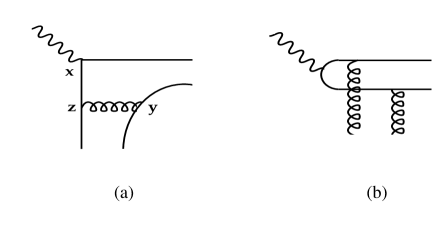
Figure 3: Typical graphs which contribute to the hard exclusive meson production amplitude.

where $t^{A}$ and $t^{B}$ denote the generators of color SU(3). As a next step we perform the usual Operator Product Expansion of ${\cal M}(x,y,z)$. Choosing, for example, the flow of the hard momentum $q$ as in Fig.3(a), we obtain a term which can be interpreted as photon-meson transition in a background quark field provided by the nucleon. In the remaining (not shown) leading order contributions the photon couples to one of the other possible quark lines. A different choice of the hard momentum flow results in a photon-meson transition in the background gluon field as shown in Fig.3(b). This gluon contribution has been discussed several times in recent papers [5, 7, 31]. We therefore outline in the following the calculation of the quark part. Here the diagram in Fig.3(a) corresponds in leading order $\alpha_{s}$ to:

$${\cal M}(x,y,z)\ni\left[\bar{\psi}^{d}(y)\,\gamma^{\sigma}\,\psi^{e}(y)\right]\left[\bar{\psi}^{c}(x)\hat{\epsilon_{L}}\,S^{q(ca)}(x-z)\,\gamma^{\rho}\,\psi^{b}(z)\right]S^{g(BA)}_{\sigma\rho}(y-z)\,t^{A}_{ab}t^{B}_{de}.$$ (35)

$S^{q}$ and $S^{g}$ stand for the quark and gluon perturbative Feynman propagators, respectively. Next we perform a Fierz transformation in color- and Dirac-space. Of course in color-space only the singlet piece survives when matrix elements between colorless hadronic initial and final states are taken. In Dirac-space we have:

$$\left[\bar{\psi}^{d}(y)\,\gamma^{\sigma}\,\psi^{e}(y)\right]\left[\bar{\psi}^{c}(x)\hat{\epsilon_{L}}\,S^{q(ca)}(x-z)\,\gamma^{\rho}\,\psi^{b}(z)\right]=\sum_{i,j}C_{ij}^{\sigma\rho}\,{\hat{O}_{i}}(y,z)\,{\hat{O}_{j}}(x,y),$$ (36)

with the operators $\hat{O}_{i}$ and ${\hat{O}_{j}}$ defined as:

$$\hat{O}_{i,j}(y,z)=\left[\bar{\psi}(y)\,\Gamma_{i,j}\,\psi(z)\right].$$ (37)

The coefficients $C_{ij}$ are given by:

$$C_{ij}^{\sigma\rho}=-\frac{1}{16}\mbox{Tr}\left[\gamma^{\sigma}\Gamma_{j}\,\hat{\epsilon}_{L}\,S^{q}(x-z)\,\gamma^{\rho}\Gamma_{i}\right],$$

$$\mbox{with}\quad\Gamma_{i,j}\in\{1,\gamma_{5},\gamma^{\mu},\gamma_{5}\gamma^{\mu},\sigma^{\mu\nu}\}.$$ (38)

For color singlet final states higher order corrections generate path-ordered exponentials which ensure gauge-invariance of the operators $\hat{O}_{i,j}$ [5]. As a next step leading twist pieces have to be extracted. In the massless limit, i.e. $P^{2}=P^{\prime 2}=q^{{}^{\prime}2}=0$, this can be achieved by using the Sudakov decomposition of $\gamma$ matrices:

$$\gamma^{\mu}=\frac{\hat{q^{\prime}}}{P\cdot q^{\prime}}\,P^{\mu}+\frac{\hat{P}}{P\cdot q^{\prime}}\,q^{\prime\mu}+\gamma_{\perp}^{\mu}.$$ (39)

Typically only longitudinal terms proportional to $P$ or $q^{\prime}$ contribute at the twist-2 level. Evaluating the corresponding trace and sandwiching operators ${\hat{O}}_{i}$ and ${\hat{O}}_{j}$ between initial and final states gives the desired amplitudes in terms of meson distribution amplitudes and nucleon nonforward parton distributions. An important outcome of this calculation is that only operators with $\Gamma_{i}=\Gamma_{j}$ contribute. Since the spin and parity of the produced meson determines the Dirac matrix in the meson amplitude, it automatically fixes the involved nonforward distribution.

5.1 Vector mesons

To leading twist accuracy two amplitudes for longitudinally and transversely polarized vector mesons exist (see [32] for a recent discussion). In the longitudinal case one has:

$$\langle M(q^{\prime})|\,\bar{\psi}(x)\hat{P}\psi(y)\,|0\rangle=q^{\prime}\cdot P\,f_{V_{L}}\int_{0}^{1}d\tau\,\Phi_{V_{L}}(\tau)\,e^{iq^{\prime}\cdot\,(\tau x+\bar{\tau}y)},$$ (40)

where $f_{V_{L}}$ and $\Phi_{V_{L}}$ denote the corresponding decay constant and distribution amplitude. According to our previous discussion this implies that the quark contribution to the production of longitudinally polarized vector mesons is determined by the nucleon matrix element $\langle N(P^{\prime})|\bar{\psi}(z)\hat{q}^{\prime}\psi(y)|N(P)\rangle$. As a consequence the nonforward quark distributions $F$ and $K$, defined in Eqs.(2.1,16), enter. The corresponding amplitude reads:

$${\cal A}^{q}_{V_{L}} = \,\pi\,\alpha_{s}\,\frac{C_{F}}{N_{c}}\frac{1}{Q}\frac{\bar{N}(P^{\prime},S^{\prime})\hat{q}^{\prime}N(P,S)}{P\cdot q^{\prime}}f_{V_{L}}\int_{0}^{1}d\tau\frac{\Phi_{V_{L}}(\tau)}{\tau\bar{\tau}}$$ (41)

$$\times \int_{0}^{1}dX\left[F_{\zeta}(X,t)+\bar{F}_{\zeta}(X,t)\right]\left(\frac{1}{X-i\epsilon}+\frac{1}{X-\zeta+i\epsilon}\right)$$

$$+ \,\pi\,\alpha_{s}\,\frac{C_{F}}{N_{c}}\frac{1}{Q}\,\frac{\bar{N}(P^{\prime},S^{\prime})(\hat{q}^{\prime}\hat{r}-\hat{r}\hat{q}^{\prime})N(P,S)}{2\,M\,P\cdot q^{\prime}}f_{V_{L}}\int_{0}^{1}d\tau\frac{\Phi_{V_{L}}(\tau)}{\tau\bar{\tau}}$$

$$\times \int_{0}^{1}dX\left[K_{\zeta}(X,t)+\bar{K}_{\zeta}(X,t)\right]\left(\frac{1}{X-i\epsilon}+\frac{1}{X-\zeta+i\epsilon}\right).$$

Since the virtual photon and the final state vector meson carry the same C-parity, vector meson production can take place also in the gluon background field. Its contribution is [5, 7, 31]:

$${\cal A}^{g}_{V_{L}} = \,2\pi\,\alpha_{s}\,\frac{1}{N_{c}}\frac{1}{Q}\frac{\bar{N}(P^{\prime},S^{\prime})\hat{q}^{\prime}N(P,S)}{P\cdot q^{\prime}}\,\left(1-\frac{\zeta}{2}\right)\,f_{V_{L}}\int_{0}^{1}d\tau\frac{\Phi_{V_{L}}(\tau)}{\tau\bar{\tau}}$$ (42)

$$\times \int_{0}^{1}dX\,\frac{G_{\zeta}(X,t)}{(X-i\epsilon)(X-\zeta+i\epsilon)}+K-\mbox{terms},$$

with $G$ being the nonforward gluon distribution (5) of the nucleon.

Transversely polarized vector mesons are described by the amplitude [32]:

$$\langle M(q^{\prime})|\,\bar{\psi}(x)\sigma_{\mu\nu}\psi(y)\,|0\rangle=-i(\epsilon_{\mu}q^{\prime}_{\nu}-\epsilon_{\nu}q^{\prime}_{\mu})f_{V_{T}}\int_{0}^{1}d\tau\,\Phi_{V_{T}}(\tau)\,e^{iq^{\prime}\cdot\,(\tau x+\bar{\tau}y)}.$$ (43)

Their production from longitudinally polarized photons involves chiral-odd nucleon nonforward parton distributions. Thus, in general, only the nonforward quark transversity distribution contributes. An explicit calculation shows, however, that in leading order $\alpha_{s}$ the twist-2 contribution vanishes and one has to go either to higher orders, or to higher-twists to obtain a non-zero result.

5.2 Pseudoscalar mesons

In the case of pseudoscalar mesons one ends up with the amplitude:

$$\langle M(q^{\prime})|\,\bar{\psi}(x)\gamma_{5}\hat{P}\psi(y)\,|0\rangle=i\,q^{\prime}\cdot P\,f_{PS}\int_{0}^{1}d\tau\,\Phi_{PS}(\tau)\,e^{iq^{\prime}\cdot\,(\tau x+\bar{\tau}y)},$$ (44)

with the meson decay constant $f_{PS}$ and the distribution amplitude $\Phi_{PS}$. According to the above discussion the production process is sensitive to the nonforward nucleon matrix element $\langle N(P^{\prime})|\bar{\psi}(z)\gamma_{5}\hat{q}^{\prime}\psi(y)|N(P)\rangle$. Thus the nonforward polarized quark distributions $\Delta F$ and $\Delta K$ from Eqs.(4,16) enter. Collecting all leading order contributions gives for the pseudoscalar meson production amplitude:

$${\cal A_{PS}}=i\,\pi\,\alpha_{s}\,\frac{C_{F}}{N_{c}}\frac{1}{Q}\frac{\bar{N}(P^{\prime},S^{\prime})\gamma_{5}\hat{q}^{\prime}N(P,S)}{P\cdot q^{\prime}}f_{PS}\int_{0}^{1}d\tau\frac{\Phi_{PS}(\tau)}{\tau\bar{\tau}}$$

$$\hskip 14.22636pt\times\int_{0}^{1}dX\left[\Delta F_{\zeta}(X,t)-\Delta\bar{F}_{\zeta}(X,t)\right]\left(\frac{1}{X-i\epsilon}+\frac{1}{X-\zeta+i\epsilon}\right)+K-\mbox{terms},$$ (45)

Due to C-parity conservation pseudoscalar meson production receives contributions only from C-odd nonforward distribution functions. As an immediate consequence two gluon exchange is impossible. At least three gluons have to be exchanged, which in the language of twist expansion corresponds to higher-twist.

6 Results

Using the derived production amplitudes together with the model distributions from Sec.3 allows to calculate the production of neutral pseudoscalar and vector mesons. In both cases we use the asymptotic meson distribution amplitude [23, 26]:

$$\Phi_{PS}(\tau)=\Phi_{V_{L}}(\tau)=6\tau(1-\tau).$$ (46)

In numerical calculations we have neglected the practically unconstrained ”$K$-terms”. As their contribution enters proportional to $r$ it is bound to be small at small momentum transfers.

6.1 $\pi^{0}$ and $\eta$ production

To obtain predictions for a specific process the generic amplitudes from Sec.5 have to be furnished with flavor charges. Using standard SU(3) wave functions for the pseudoscalar meson octet implies for $\pi^{0}$ and $\eta$ production an replacement of the nonforward distributions in Eq.(45) through distributions with specific flavor as listed in Tab.1.

	$\Delta F_{\zeta}(X,t)-\Delta\bar{F}_{\zeta}(X,t)$
$\rule[-8.53581pt]{0.0pt}{22.76219pt}\pi^{0}$	$\sqrt{2}\left[\frac{1}{3}\,(\Delta u_{\zeta}-\Delta\bar{u}_{\zeta})+\frac{1}{6}\,(\Delta d_{\zeta}-\Delta\bar{d}_{\zeta})\right]$
$\rule[-8.53581pt]{0.0pt}{22.76219pt}\eta$	$\sqrt{6}\left[\frac{1}{9}\,(\Delta u_{\zeta}-\Delta\bar{u}_{\zeta})-\frac{1}{18}\,(\Delta d_{\zeta}-\Delta\bar{d}_{\zeta})+\frac{2}{9}\,(\Delta s_{\zeta}-\Delta\bar{s}_{\zeta})\right]$

Table 1: Flavor structure for $\pi^{0}$ and $\eta$ production. Analogous relations hold for the $"K-\mbox{terms}"$.

For $\pi^{0}$ production we use the standard value for the decay constant $f_{\pi}=133$ MeV. In Fig.4 we present the corresponding differential production cross section for a proton target taken at $t=t_{\min}=-x_{Bj}^{2}M^{2}/(1-x_{Bj})$. We restrict ourselves to the region $|t_{min}|<1$ GeV², which implies $x_{Bj}<0.6$.

One finds that, up to logarithmic corrections, the production cross section drops as $1/Q^{6}$. Furthermore, at small values of $x_{Bj}$ the calculated cross section is proportional to $x_{Bj}^{2\lambda}$ with $\lambda\approx 0.6$. This behavior is controlled by the small-$x_{Bj}$ behavior of the polarized valence quark distributions which enter in Eq.(21). For the used parametrizations from Ref.[24] one has indeed $x_{Bj}\Delta u_{v}(x_{Bj})\sim x_{Bj}\Delta d_{v}(x_{Bj})\sim x_{Bj}^{\lambda}$. The decrease of the production cross section at large $x_{Bj}$ is due to the form factor in Eq.(21). It is important to note that this behavior should be quite general and largely independent of a specific model for double distributions. The reason is that the rise of the production cross section with increasing $x_{Bj}$ is brought to an end through the decrease of the involved nonforward or double distributions at large momentum transfers $|t|$. Since the latter is determined by a typical nucleon scale, $\Lambda\sim 1$ GeV, the maximum of the pseudoscalar meson production cross section at $t=t_{min}$ should occur when $t_{min}$ starts to become sizeable, say $-t_{min}/\Lambda^{2}\mathrel{\raise 2.58334pt\hbox{$>$}\kern-7.7778pt\lower 2.79857pt\hbox{$\sim$}}0.2$. This implies $x_{Bj}\approx 0.3$ in accordance with our result.

Our prediction for the $\eta$ production cross section turns out to be approximately a factor $2/3$ smaller than for $\pi^{0}$, but of similar shape. This is due to the comparable shape of the polarized $u$ and $d$ valence quark distributions from Ref.[24] which enter in Eq.(21).

6.2 Vector meson production

For $\rho^{0},\Phi$ and $\omega$ production the nonforward distributions in Eq.(41,42) have to be modified according to Tab.2

	$F_{\zeta}(X,t)+\bar{F}_{\zeta}(X,t)$	$G_{\zeta}(X,t)$
$\rule[-8.53581pt]{0.0pt}{22.76219pt}\rho^{0}$	$\sqrt{2}\left[\frac{1}{3}\,(u_{\zeta}+\bar{u}_{\zeta})+\frac{1}{6}\,(d_{\zeta}+\bar{d}_{\zeta})\right]$	$\frac{1}{\sqrt{2}}\,G_{\zeta}$
$\rule[-8.53581pt]{0.0pt}{22.76219pt}\omega$	$\sqrt{2}\left[\frac{1}{3}\,(u_{\zeta}+\bar{u}_{\zeta})-\frac{1}{6}\,(d_{\zeta}+\bar{d}_{\zeta})\right]$	$\frac{1}{3\sqrt{2}}\,G_{\zeta}$
$\rule[-8.53581pt]{0.0pt}{22.76219pt}\Phi$	$-\frac{1}{3}\,(s_{\zeta}+\bar{s}_{\zeta})$	$-\frac{1}{3}\,G_{\zeta}$

Table 2: Flavor structure for $\rho^{0}$, $\omega$ and $\Phi$ meson production.

In the kinematic domain of small $x_{Bj}<0.01$ the quark part of the production amplitude (41) is negligible. Then the well known SU(3) relation for the cross section ratios $\sigma(\rho):\sigma(\omega):\sigma(\Phi)=9:1:2$ follows immediately from Tab.2.

In Ref.[10, 11, 12] hard exclusive neutral vector meson production has been investigated at small values of $x_{Bj}$ within the framework of perturbative QCD. In this work the nonforward gluon distribution which, in general, enters the production amplitude (42) has been approximated by the ordinary gluon distribution. In the limit of small $x_{Bj}$ the obtained amplitude corresponds to Eq.(42) after the replacement $G_{\zeta}(\zeta,t)\rightarrow\zeta\,g(\zeta)$, where $g$ denotes the ordinary gluon distribution. However, note that for a typical behavior of the gluon double distribution $G(x,y,t)\sim x^{-\lambda}$ with $\lambda>0$ one obtains from Eq.(3) for the ratio:

$$\frac{G_{\zeta}(\zeta,t=0)}{\zeta g(\zeta)}\approx 1+\lambda\,\frac{\int_{0}^{1}dy\,y\,G(\zeta,y,t=0)}{\int_{0}^{1}\,dy\,G(\zeta,y,t=0)}>1.$$ (47)

For our model distribution from Sec.3 this leads to an increase of the vector meson production cross sections by nearly a factor of two as compared to the results of [12].

It should be mentioned that the leading order calculations from Refs.[10, 11, 12] overestimate the experimental data from HERA [9] by a typical factor $5-10$. Additional Fermi motion corrections have been added to fit experimental data. This emphasizes the need for a systematic investigation of higher twist effects [31].

In Fig.5 we present the result for $\rho^{0}$ production from a proton in the kinematic domain of HERA [33] as obtained from the amplitudes in Eqs.(41,42), combined with the double distributions from Sec.3. For the $\rho$ meson decay constant $f_{\rho}=216$ MeV has been used. After multiplying with a suppression factor $T(Q^{2}=16.9\,\mbox{GeV}^{2})\approx 0.1$ from [12] qualitative agreement can be achieved.

Finally we would like to note that special attention should be paid to exclusive charged meson production. Here at large $Q^{2}$ nonforward parton distributions are probed which are related to matrix elements of twist-2 non-local operators off diagonal in flavor:

$${\hat{O}}_{qq^{\prime}}(x,y)=\bar{q}(x)\,\Gamma\,q^{\prime}(y),$$ (48)

with flavor dependent quark fields, $q=u,d,s$. As a consequence hard exclusive charged meson production offers possibilities to explore exotic parton distributions which have not been measured elsewhere. These obey isospin symmetry relations analogous to the Bjorken sum rule known from polarized deep-inelastic scattering:

$$\langle n|{\hat{O}}_{du}(x,y)|p\rangle = \langle p|{\hat{O}}_{uu}(x,y)|p\rangle-\langle p|{\hat{O}}_{dd}(x,y)|p\rangle,$$

$$\langle n|{\hat{O}}_{du}(x,y)|p\rangle = \langle n|{\hat{O}}_{dd}(x,y)|n\rangle-\langle n|{\hat{O}}_{uu}(x,y)|n\rangle.$$ (49)

Here $\langle n|$ and $\langle p|$ denote neutron and proton states, respectively. These sum rules imply a close relation of charged meson production cross sections. They allow, for example, to relate the isovector part of the amplitude for $\rho^{0}$ production to a linear combination of $\rho^{+}$ and $\rho^{-}$ production amplitudes.

7 Summary

Ordinary parton distributions accessible e.g., in deep-inelastic scattering measure the nucleon response to a process where one parton is removed and subsequently inserted back into the target along a light-like distance, without changing its longitudinal momentum. Generalized parton distributions, so-called nonforward distributions, can be studied in deeply virtual Compton scattering and hard exclusive leptoproduction of mesons. They describe a situation where the removed parton changes its longitudinal momentum before returning to the nucleon. Furthermore, hard exclusive charged meson production provides possibilities to investigate new processes where the removed quark carries different flavor than the returning one.

In this paper we have studied general properties of double and nonforward parton distributions. We have found a symmetry of quark and gluon double distribution functions based on their relation to nonforward matrix elements of QCD string operators. Its implication for phenomenological models has been outlined.

Although the leading order QCD evolution equations seem to be more complicated in the non-forward than in the forward case, one can solve them explicitly using an expansion in a set of orthogonal polynomials instead of performing a Mellin integral in the complex plane of distribution function moments. We have outlined this method for the flavor nonsinglet case. A generalization to flavor singlet distributions is possible.

In the second half of this paper we have derived the amplitudes for the hard exclusive production of neutral mesons from longitudinally polarized photons. After suggesting a phenomenological model for double or nonforward distribution functions which obey appropriate symmetries, we have presented results for exclusive $\pi^{0}$, $\eta$ and $\rho^{0}$ production.

In the pseudoscalar case nonforward polarized valence quark distributions enter. Several features of the presented results should be independent of our specific model for nonforward distribution functions: at small $x_{Bj}$ pseudoscalar meson production cross sections drop for decreasing $x_{Bj}$. This is related to a similar behavior of the corresponding forward distributions. Furthermore, the production cross sections peak at moderate $x_{Bj}$. This is due to the dependence of the involved nonforward distributions on the momentum transfer which should be controlled by a typical nucleon scale.

We also have presented results for $\rho^{0}$ production in the kinematic domain of recent HERA measurements. Here the production process is dominated by contributions from the nonforward gluon distribution. For a large class of model distributions this tends to be larger than the corresponding forward distribution.

Acknowledgments: We gratefully acknowledge discussions with W. Melnitchouk and A. Radyushkin. This work was supported in part by BMBF, KBN grant 2 P03B 065 10, and German-Polish exchange program X081.91.

Figure 1: Polarized $u$-valence distribution ${\Delta u}_{\zeta}(X;\mu^{2}=4)$ from Eq.(21) for different values of $\zeta$.

Figure 2: Evolution of the nonforward polarized $u$-valence distribution ${\Delta u}_{\zeta=0.2}(X;\mu^{2})$ for different values of $\mu^{2}$.

Figure 4: Differential cross section for exclusive $\pi^{0}$ production from protons at $t=t_{min}$.

Figure 5: Cross section for $\rho^{0}$ production from a proton through the interaction of longitudinally polarized photons. The data are taken from ZEUS [33] (open squares) and NMC [34] (filled circles).

References

-
[1]
J. Bartels and M. Loewe, Z. Phys. C12, 263 (1982);
L. Gribov, E. Levin and M. Ryskin, Phys. Rep. 100, 1 (1983). -
[2]
B. Geyer, D. Robaschik, M. Bordag and J. Horejsi,
Z. Phys. C26, 591 (1985);
F.-M. Dittes et al., Phys. Lett. B209, 325 (1988);
F.-M. Dittes et al., Fortschr. Phys. 42, 101 (1994). - [3] P. Jain and J. Ralston, Proceedings of the Workshop on Future Directions in Particle and Nuclear Physics at Multi-GeV Hadron Beam Facilities, Brookhaven National Laboratory, Upton, NY, 1993.
-
[4]
X. Ji, Phys. Rev. D55, 7114 (1997);
X. Ji, Phys. Rev. Lett. 78, 610 (1997). -
[5]
A. Radyushkin, Phys. Lett. B380, 417 (1996);
A. Radyushkin, Phys. Lett. B385, 333 (1996);
A. Radyushkin, Phys. Rev. D56, 5524 (1997). - [6] J. Collins and D. Soper, Nucl. Phys. B194, 445 (1982).
- [7] P. Hoodbhoy, Phys. Rev. D56, 338 (1997).
- [8] J. Collins, L. Frankfurt and M. Strikman, Phys. Rev. D56, 2982 (1997).
- [9] J. Crittenden, Tracts in Modern Physics, Volume 140, Springer, 1997.
- [10] M. Ryskin, Z. Phys. C57, 89 (1993).
- [11] S. Brodsky et al., Phys. Rev. D50, 3134 (1994).
- [12] L. Frankfurt, W. Koepf and M. Strikman, Phys. Rev. D54, 3194 (1996).
- [13] A. Martin, M. Ryskin and T. Teubner, Phys. Rev. D55, 4329 (1997).
- [14] L. Frankfurt, A. Freund, V. Guzey and M. Strikman, Nondiagonal parton distribution in the leading logarithmic approximation, 1997, hep-ph/9703449.
- [15] see e.g. C. Carlson, Nucl. Phys. A622, 66c (1997).
- [16] G. van der Steenhoven, Future physics with light and heavy nuclei at HERMES, Proceedings of the Workshop “Future Physics at HERA”, Hamburg 1996.
- [17] G. Baum et al., COMPASS proposal, CERN-SPSLC-96-14, 1996.
- [18] V. Braun, P. Górnicki, L. Mankiewicz and A. Schäfer, Phys. Lett. B302, 291 (1993).
-
[19]
X. Ji, W. Melnitchouk and X. Song, A study of off forward parton
distributions, 1997, hep-ph/9702379 ;
V. Petrov, P. Pobylitsa, M. Polyakov, I. Börning, K. Goeke and C. Weiss, Off-forward quark distributions of the nucleon in the large limit, 1997, hep-ph/9710270. - [20] P. Collins, An Introduction to Regge Theory and High-Energy Physics, Cambridge University Press, 1977.
- [21] A. Radyushkin, private communication.
- [22] T. Ericson and W. Weise, Pions and Nuclei, Oxford University Press, 1988.
- [23] G. Lepage and S. Brodsky, Phys. Rev. D22, 2157 (1980).
- [24] T. Gehrmann and W.J. Stirling, Phys. Rev. D53, 6100 (1996).
-
[25]
I. Balitskii and V. Braun, Nucl. Phys. B311, 541 (1988/89);
J. Blümlein, B. Geyer and D. Robaschik, On the Evolution Kernels of Twist-2 Light Ray Operator for Unpolarized and Polarized Deep Inelastic Scattering, 1997, hep-ph/9705264;
I. Balitskii and A. Radyushkin, Light Ray Evolution Equations and Leading Twist Parton Helicity Dependent Nonforward Distributions, 1997, hep-ph/9706410. -
[26]
A. Efremov and A. Radyushkin, JINR-E2-11535, Dubna, 1978;
A. Efremov and A. Radyushkin, Theor. Math. Phys. 42, 97 (1980). -
[27]
M. Chase, Nucl. Phys. B167, 125 (1980);
M. Chase, Nucl. Phys. B174, 109,(1980);
T. Ohrndorf, Nucl. Phys. B198, 26 (1982);
D. Müller, Restricted conformal invariance in QCD and its predictive power for virtual two-photon processes, 1997, hep-ph/9704406;
A. Belitsky, D. Müller, Predictions from conformal algebra for the deeply-virtual compton scattering, 1997, hep-ph/9709379. - [28] T. Weigl and W. Melnitchouk, Nucl. Phys. B465, 267 (1996).
- [29] V. Krylov and N. Skoblya, Handbook of numerical inversion of Laplace transforms, Jerusalem, 1969.
- [30] A. Belitsky, B. Geyer, D. Müller and A. Schäfer, On the leading logarithmic evolution of the off-forward distributions, 1997, hep-ph/9710427.
- [31] I. Halperin and A. Zhitnitsky, Phys. Rev. D56, 184 (1997).
- [32] P. Ball and V. Braun, Phys. Rev. D54, 2182 (1996).
- [33] M. Derrick et al., Phys. Lett. B356, 601 (1995).
- [34] M. Arneodo et al., Nucl. Phys. B429 (1994) 503.