Theory of Jets in Deep Inelastic Scattering
Erwin Mirkes
Institut für Theoretische Teilchenphysik, Universität Karlsruhe,
D-76128 Karlsruhe, Germany
Abstract

The large center of mass energy and increasing statistical precision for a wide range of hadronic final state observables at the HERA lepton-proton collider has provided a detailed testing ground for QCD dynamics. Fully flexible next-to-leading order calculations are mandatory on the theoretical side for such tests and will be discussed in detail. Next-to-leading order QCD predictions for one- and two-jet cross sections in deep inelastic scattering with complete neutral current ($\gamma^{\ast}$ and/or $Z$) and charged current ($W^{\pm}$) exchange together with leading order results for three- and four-jet final states are presented. The theoretical framework, based on the phase space slicing method and the use of universal crossing functions, is described in detail. All analytical formulae necessary for the next-to-leading order calculations are provided. The numerical results are based on the fully differential $ep\rightarrow n$ jets event generator mepjet which allows to analyze any infrared and collinear safe observable and general cuts in terms of parton 4-momenta. The importance of higher order corrections is studied for various jet algorithms. Implications and comparisons with (ongoing) experimental analyses for jet cross sections at high $Q^{2}$, the determination of $\alpha_{s}(\mu_{R})$, the gluon density, power corrections in event shapes and the associated forward jet production in the low $x$ regime at HERA are discussed. A study of jet cross sections in polarized electron and polarized proton collisions shows that dijet events provide a good measurement of the polarized gluon distribution $\Delta g(x_{g})$, in a region, where $x_{g}\Delta g(x_{g})$ is expected to show a maximum.

To Caroline

1 Introduction

Deep inelastic lepton-nucleon scattering has played an important role in our present understanding of the structure of matter. Early fixed target experiments [1] have established the partonic structure of the nucleon and contributed essentially to the development of Quantum Chromodynamics (QCD), the theory that describes the strong interaction of quarks and gluons, collectively known as partons. The start-up of the HERA lepton-proton collider in 1992 with a center of mass energy of $\sqrt{s}\approx 300$ GeV (27.5 GeV positrons on 820 GeV protons) marked the beginning of a new era of experiments exploring deep inelastic scattering (DIS). While the traditional method of obtaining information on the parton structure of the nucleon is through measurements of inclusive (w.r.t. the hadronic final state) structure functions, increasingly precise data from HERA for a wide range of hadronic final state variables became availabe and provide a considerably more detailed testing ground for the strong interaction.

The physics of the hadronic final state in DIS, and in particular the study of multi-jet events and event shapes, has in fact become one of the main interests at HERA. Topics to be studied include the measurement of the strong coupling constant from jet rates and event shapes, the measurement of the gluon density from dijet events, the study of power-suppressed corrections to event shapes and the search for new physics at small $x$ in associated forward jet production and in 1-jet inclusive events at very high $Q^{2}$.

On the theoretical side, versatile next-to-leading order (NLO) QCD calculations are mandatory for these studies. Based on significant recent theoretical progress, such a fully flexible NLO calculation became available for arbitrary infrared-safe observables (1- and 2-jet-like quantities) in DIS [2, 3]. In general, such calculations are highly non-trivial. The main theoretical problem is the occurance of severe infrared and/or collinear divergencies. However, any physical hadronic final state observable must be infrared safe and either collinear safe or collinear factorizable, i.e. the singularities ultimately cancel or are factorized into process-independent physical parton distribution or fragmentation functions. In this review, we present a detailed description of the theoretical framework for the calculation together with a comparison of the theoretical expectations with a variety of recent experimental results at HERA.

Why is it essential to work at least to NLO to make quantitative predictions in perturbative QCD, and in particular in jet physics? Leading order (LO) calculations rely on tree level matrix elements and therefore provide only a basic description of cross sections and distributions, but are sensitive to potentially large, but uncalculated ultraviolet and infrared logarithms. In a NLO calculation, the virtual corrections (initial state collinear factorization in the bremsstrahlung contributions) introduce an explicit logarithmic dependence on the renormalization scale $\mu_{R}$ (factorization scale $\mu_{F}$), which substantially reduces the $\mu_{R}$ ($\mu_{F}$) scale dependence present in the LO calculation. In addition, infrared logarithms from the NLO bremsstrahlung contributions introduce an explicit logarithmic dependence on the jet-defining parameters through the presence of real radiation inside a jet or soft real radiation outside a jet.

NLO corrections in jet physics imply furthermore that a jet (in a given jet definition scheme) may consist of two partons. Thus first sensitivity to the partition of particles in a jet and therefore the internal jet structure is obtained, such as the dependence on the cone size or on recombination prescriptions. Such studies give interesting information about the process by which hard partons are confined into jets of hadrons.

Full NLO corrections for 1-jet and 2-jet cross sections and distributions in DIS $e^{\pm}p$ scattering with complete neutral current ($\gamma^{\ast}$ and/or $Z$) and charged current ($W^{\pm}$) exchange are discussed. All analytical formulae necessary for the NLO order QCD calculations are provided. The numerical results are based on the $ep\rightarrow n$ jets event generator mepjet [2, 3], which also allows for the calculation of LO 3-jet and 4-jet differential cross sections including $W$ and $Z$ exchange. In addition, charm and bottom quark mass effects can be taken into account for LO 1-, 2- and 3-jet results with $\gamma^{\ast}$ exchange. The matrix elements are derived by using spinor helicity methods [4, 5, 6]. Thus the full spin structure is kept in the calculation and so mepjet allows for the calculation of all possible jet-jet and jet-lepton correlations as well as for the calculation of jet cross sections in polarized electron and polarized proton collisions.

Jet studies on the experimental (hadronic) and theoretical (partonic) level require an exact definition of resolvable jets, which is usually given in terms of one or more resolution parameters and a recombination scheme description of how to combine clusters of particles or jets which do not fulfill the resolution criteria. A good jet algorithm will have small higher order corrections, small hadronization corrections and a small recombination scheme dependence. An important goal of a versatile NLO calculation is to allow for an easy implementation of arbitrary jet algorithms together with the chosen recombination scheme and to impose any kinematical resolution and acceptance cuts on the final state particles. This is best achieved by performing all hard phase space integrals numerically, with a Monte Carlo integration technique, which in fact allows to analyze any infrared and collinear safe observable and general cuts in terms of parton 4-momenta.

The results for the NLO jet cross sections in this paper are based on the “phase space slicing” method ($s_{\mbox{\scriptsize min}}$-technique) [6, 7, 8] and on the technique of universal crossing functions [9]. An invariant theoretical resolution parameter $s_{\mbox{\scriptsize min}}$ is introduced to isolate the infrared (soft) as well as collinear divergencies associated with the unresolved regions where at least one pair of partons, including initial ones, has $s_{ij}=2p_{i}\cdot p_{j}<s_{\mbox{\scriptsize min}}$. Integrating analytically over the soft and/or collinear final state parton allows to cancel the soft and collinear divergencies against the corresponding divergencies in the virtual contributions and to factorize the remaining collinear initial state divergencies into the bare parton densities (see section 2 for a detailed discussion). The integration over the finite resolved phase space with $s_{ij}>s_{\mbox{\scriptsize min}}$ is done numerically, by Monte-Carlo techniques, and, thus, the parton 4-momenta are available at each phase space point. As a result the program is flexible enough to implement arbitrary jet algorithms and kinematical resolution and acceptance cuts. Upon adding the resolved and unresolved contributions the dependence on the resolution parameter $s_{\mbox{\scriptsize min}}$ disappears (in the limit $s_{\mbox{\scriptsize min}}\rightarrow 0$) and one obtains the NLO fully differential cross section.

The 1-jet final state is the most basic high transverse momentum event at HERA, with a lepton and a jet back-to-back in the transverse plane. In lowest order ($\alpha_{s}^{0}$), the underlying partonic process, $e^{\pm}$-quark scattering, is completely fixed by the Standard Model electroweak interactions. Although the NLO matrix elements for this parton model process have been known for a long time [10], including electroweak exchange [11], mepjet is currently the only program that allows to calculate the NLO 1-jet or NLO total inclusive cross sections including all electroweak effects, in the presense of arbitrary acceptance cuts on the final state lepton (or jet).

One-jet and total cross sections at $\mbox{$\cal{O}$}(\alpha_{s})$ are of particular interest as a normalizer for jet rates. In addition, both HERA experiments have recently reported an excess of $e^{+}p$ neutral current 1-jet (inclusive) events above Standard Model predictions. The excess amounts to about a factor two increase in rate at large values of $Q^{2}$ ($Q^{2}>1.5\times 10^{4}$ GeV²) [12], and has led to speculations on evidence for new physics (see e.g. Ref. [13] and references therein). The full 1-loop corrections in this high $Q^{2}$-region are investigated in section 4.3.

The properties of jet events can be studied in much greater depth in final states with 2 or more jets. In Born approximation, the subprocesses $eq\rightarrow eqg$, $e\bar{q}\rightarrow e\bar{q}g$ and $eg\rightarrow eq\bar{q}$ contribute to the 2-jet cross section [14, 11]. A large variety of issues can be adressed with these processes, and in all cases the availability of NLO corrections is necessary to move such studies from the qualitative level to precision studies of QCD effects. The list of topics which can be studied quantitatively, once NLO corrections for the complete neutral current and charged current exchange processes are available, include the following:
i) The determination of $\alpha_{s}(\mu_{R})$ over a range of scales $\mu_{R}$ from dijet production:
The dijet cross section is proportional to $\alpha_{s}(\mu_{R})$ at LO, thus suggesting a direct measurement of the strong coupling constant. However, the LO calculation leaves the renormalization scale $\mu_{R}$ undetermined. The NLO corrections substantially reduce the dependence of the cross section on the renormalization scale and thus reliable cross section predictions in terms of $\alpha_{s}(m_{Z})$ are made possible. An important issue which must be addressed in such an $\alpha_{s}$ determination is the appropriate choice of the renormalization scale $\mu_{R}$ and the factorization scale $\mu_{F}$ in DIS jet production. The chosen scale should be characteristic for the QCD portion of the process at hand, and this typically is not the momentum transfer to the scattered lepton. The “natural” scale choice for $n$-jet production in DIS appears to be the average $k_{T}^{B}$ of the jets in the Breit frame [15, 16], as will be discussed in sections 5.3.2-5.3.7.
ii) The measurement of the gluon density in the proton (via $eg\to eq\bar{q}$):
The boson gluon fusion subprocess $\mbox{boson}+g\rightarrow q+\bar{q}$, which enters already at LO, dominates the 2-jet cross section at low and medium Bjorken-$x$ and allows for a direct measurement of the gluon density $g(\xi,\mu_{F})$. The momentum fraction $\xi$ is related to $x$ by $\xi=x(1+m_{jj}^{2}/Q^{2})$, where $m_{jj}$ is the invariant mass of the produced dijet system. NLO corrections reduce the factorization scale $\mu_{F}$ dependence in the LO calculation due to the initial state collinear factorization, which introduces a mixture of the quark and gluon densities according to the Altarelli-Parisi evolution. Thus reliable cross section predictions in terms of the scale dependent parton distributions are made possible [3]. The “natural” choice for $\mu_{F}$ is again given by the average $k_{T}^{B}$ of the jets in the Breit frame (see section 5.3.7).
iii) Power corrections in event shapes:
Recent theoretical developments in the understanding of infrared renormalon contributions, which lead to deviations from the perturbative calculation, allow the first steps towards a direct comparison of theory and data without invoking hadronization models. These power corrections, with a characteristic $1/Q$ dependence, can be calculated for event shape variables [17] and differential jet rates. Comparing data directly with NLO theory, which is augmented by the calculated power corrections, allows to fix the nonperturbative parameters which characterize the size of these power corrections [18]. Having constrained the hadronization corrections in this way allows also for a precise extraction of $\alpha_{s}$, which is expected to be less sensitive to hadronization uncertainties (see section 5.3.9).
iv) Probing the full hadronic structure via lepton-hadron correlations:
Lepton-hadron correlations provide a unique opportunity to analyze the hadronic production mechanism in more detail than is possible by analyzing jet production cross sections alone. In the absence of jet cuts in the laboratory frame, the full QCD matrix elements predict a typical azimuthal distribution of the jets of the form

$$\frac{d\sigma}{d\phi}=A+B\cos\phi+C\cos 2\phi+D\sin\phi+E\sin 2\phi\;.$$ (1)

Here $\phi$ denotes the azimuthal angle of the jets around the virtual boson direction (in the Breit or hadronic center of mass frame), where the lepton plane defines $\phi=0^{\circ}$. This angular distribution is determined by the gauge boson polarization: the coefficients $A,B,C,D,E$ are linearly related to the nine polarization density elements of the exchanged gauge boson and a measurement of the coefficients reveals first sensitivity to the non-diagonal polarization density elements (see sections 5.1 and 5.3.4).
v) Associated forward jet production in the low $x$ regime as a signal of BFKL dynamics:
Recently, much interest has been focused on the small Bjorken-$x$ region, where one would like to distinguish the Balitsky-Fadin-Kuraev-Lipatov (BFKL) from the traditional Altarelli-Parisi (DGLAP) evolution. BFKL evolution can be enhanced and DGLAP evolution suppressed by studying DIS events which contain an identified jet with large longitudinal momentum fraction compared to Bjorken-$x$. BFKL evolution leads to a larger cross section for such events than the DGLAP evolution. A conventional fixed order QCD calculation up to ${\cal O}(\alpha_{s}^{2})$ does not yet contain any BFKL resummation and must be considered a background for its detection. Clearly, NLO QCD corrections for fixed order QCD, with DGLAP evolution, are mandatory on the theoretical side in order to establish a signal for BFKL evolution in the data [19, 20]. A detailed discussion of these fixed order effects is presented in section 7.
vi) The determination of the polarized gluon structure function (via $eg\to eq\bar{q}$) in polarized electron on polarized proton scattering:
The measurement of the polarized parton densities and in particular the polarized gluon density would allow to discriminate between the different pictures of the proton spin underlying these parametrizations. The measurement of the 2-jet final state at the HERA collider, in a scenario where both the electron and proton beams are polarized, would allow for a unique determination of the polarized gluon distribution $\Delta g(\xi,\mu_{F})$. As in the unpolarized case, the polarized gluon distribution enters the 2-jet cross section at LO suggesting such a direct measurement. The size of the expected 2-jet spin asymmetry, which is dominated by the polarized gluon initiated subprocess, can reach a few percent [21] and is thus much larger than asymmetries based on more inclusive observables. The prospects for such a measurement are discussed in section 8.
Beyond these studies, which concern the 2-jet final state, higher jet multiplicities, i.e. 3-jet and 4-jet final states in DIS, provide further interesting laboratories of perturbative QCD. ${\cal{O}}(\alpha_{s}^{3})$ 4-jet events, for example, are first sensitive to BFKL resummation effects (see section 7). Results for $n$-jet rates ($n=1,2,3,4$) as a function of $y_{\mbox{\scriptsize cut}}$ in the JADE and the $k_{T}$ jet algorithms are presented in section 6.

The numerical results in this paper can be easily reproduced by running the mepjet-program, which can be obtained from the author (see Appendix C). A documentation of mepjet version 2.1 is given in Appendix C.

A second fully flexible NLO calculation for dijet production in the one-photon exchange approximation has become available with the disent program [22], which is based on the “exact subtraction method” as described in Ref. [23]. Very recently a third calculation, disaster++, has been provided in Ref. [24], but is again restricted to the one-photon approximation. Comparisons between these calculations in the one-photon approximation yielded so far satisfactory agreement [25, 24].

The overall organization of this paper is as follows:

The general structure of NLO $n$-jet cross sections in DIS based on the crossing function and phase space slicing techniques is described in detail in section 2, which also establishes our basic notation. Some commonly used jet definitions in DIS are introduced in section 3. Analytical formulae necessary for the NLO calculations for 1-jet cross section are presented in section 4 together with a discussion of numerical results. Special emphasis is put on the calculation of the total inclusive (w.r.t. the hadronic activity) cross section and its relation to the 1-jet inclusive cross section when typical acceptance cuts on the scattered lepton are imposed. We also show that choosing $Q$ for the hard scattering scale in the $k_{T}$ jet algorithm (see section 3 for the definition) is not an infrared safe choice in the 1-jet case.

Two-jet cross sections are presented in detail in section 5. After a discussion of the exchanged gauge boson polarization effects in section 5.1, we present all analytical formulae necessary for the NLO 2-jet calculations in sections 5.2 and 5.4. A careful investigation of numerical effects in section 5.3 includes a discussion of charm and bottom quark mass effects, single jet mass effects and recombination scheme dependences, dijet azimuthal angular decorrelations, the determination of $\alpha_{s}(\mu_{R})$, the gluon density, and power corrections in event shapes. Three-jet and 4-jet cross section are presented in section 6. A full ${\cal O}(\alpha_{s}^{2})$ calculation of the inclusive forward jet cross section is presented and compared to the expected BFKL cross section in section 7. Prospects for measuring the polarized gluon density $\Delta g$ from jets at HERA with polarized electrons and protons are presented in section 8. Conclusions and outlook are given in section 9. Finally, there are three Appendices. In the first part we provide tree level and one-loop helicity amplitudes for the 2-parton final state processes in the Weyl-van der Waerden formalism. The second one explains the crossing function technique for the simplest example of the NLO 1-jet cross section. The last part of the appendix contains a documentation of the mepjet program (version 2.1).

2 NLO Jet Cross Sections in DIS

2.1 Introductory Remarks

Deep inelastic neutral current (NC) lepton proton scattering with several partons in the final state (see Fig. 1),

$$e^{\pm}(l)+\mbox{proton}(P)\rightarrow e^{\pm}(l^{\prime})+\mbox{proton remnant}(p_{r})+\mbox{parton}\,\,1(p_{1})\ldots+\mbox{parton}\,\,n(p_{n})$$ (2)

proceeds via the exchange of an intermediate vector boson $\gamma^{\ast},Z$. The charged current (CC) reaction with $e^{-}$ ($e^{+}$) on the r.h.s. of Eq. (2) replaced by $\nu_{e}$ ($\bar{\nu}_{e}$) is mediated by the exchange of a $W^{-}$ ($W^{+}$) boson. We denote the exchanged boson-momentum by $q$, its absolute square by $Q^{2}$, the center of mass energy by $\sqrt{s}$, the square of the final hadronic mass by $W^{2}$ and use the standard scaling variables $x$ and $y$ (the proton mass is neglected throughout):

$$q = l-l^{\prime}$$

$$Q^{2} \equiv -q^{2}=xys>0$$

$$s = (P+l)^{2}$$

$$W^{2} \equiv P_{f}^{2}=(P+q)^{2}$$ (3)

$$x = \frac{Q^{2}}{2Pq}\hskip 28.45274pt(0<x\leq 1)$$

$$y = \frac{Pq}{Pl}\hskip 28.45274pt(0<y\leq 1)$$

At fixed s, only two variables are independent, since

$$xW^{2}=(1-x)Q^{2},\hskip 28.45274ptQ^{2}=xys.$$

Figure 1: DIS $n$ parton production in the parton model.

The NLO $n$-jet cross section can be described in an intuitively appealing way in the framework of the QCD improved parton model [26]

$$d\sigma_{\mbox{\scriptsize had}}[n\mbox{-jet}]=\sum_{a}\int d\eta\,\,f_{a}(\eta,\mu_{F})\,\,\,\mbox{$\alpha_{s}$}^{n}(\mu_{R})\,\,\hat{\sigma}_{a}(p_{0}=\eta P,\mu_{R},\mu_{F})$$ (4)

where one sums over $a=q,\bar{q},g$. $f_{a}(\eta,\mu_{F})$ is the probability density to find a parton $a$ with fraction $\eta$ in the proton if the proton is probed at a scale $\mu_{F}$. $\hat{\sigma}_{a}$ denotes the NLO differential partonic cross section with $\alpha_{s}$ set to one from which collinear initial state singularities have been factorized out at a scale $\mu_{F}$ and have been implicitly included in the scale dependent parton densities $f_{a}(\eta,\mu_{F})$. The following tree level and one loop subprocesses contribute to $n$-jet production (up to NLO for $n=1,2$ and LO for $n=1,2,3,4$):

$$\begin{array}[]{lllll}\mbox{1-jet:}&\mbox{LO}&{\cal{O}}(\alpha_{s}^{0}):&e+q\rightarrow e+q&\mbox{}\\[2.84526pt] \mbox{1-jet:}&\mbox{NLO}&{\cal{O}}(\alpha_{s}):&e+q\rightarrow e+q&\mbox{1-loop corrections}\\ \mbox{}&&&\mbox{+ unresolved contributions from the ${\cal{O}}(\mbox{$\alpha_{s}$})$}&\mbox{2-parton final states }\\ \mbox{2-jets:}&\mbox{LO}&{\cal{O}}(\alpha_{s}):&e+q\rightarrow e+q+g&\\ \mbox{}&&&e+g\rightarrow e+q+\bar{q}&\\ \mbox{2-jets:}&\mbox{NLO}&{\cal{O}}(\alpha_{s}^{2}):&e+q\rightarrow e+q+g&\mbox{1-loop corrections}\\ \mbox{}&&&e+g\rightarrow e+q+\bar{q}&\mbox{1-loop corrections}\\ \mbox{}&&&\mbox{+ unresolved contributions from the ${\cal{O}}(\alpha_{s}^{2})$}&\mbox{3-parton final states }\\ \mbox{3-jets:}&\mbox{LO}&{\cal{O}}(\alpha_{s}^{2}):&e+q\rightarrow e+q+g+g&\\ \mbox{}&&&e+q\rightarrow e+q+q+\bar{q}&\\ \mbox{}&&&e+g\rightarrow e+q+\bar{q}+g\\ \mbox{4-jets:}&\mbox{LO}&{\cal{O}}(\alpha_{s}^{3}):&e+q\rightarrow e+q+g+g+g&\\ \mbox{}&&&e+q\rightarrow e+q+q+\bar{q}+g&\\ \mbox{}&&&e+g\rightarrow e+q+\bar{q}+g+g&\mbox{}\\ \mbox{}&&&e+g\rightarrow e+q+\bar{q}+q+\bar{q}&\\ \end{array}$$ (5)

and the crossing related anti-quark processes with $q\leftrightarrow\bar{q}$. The results for the NLO $n$-jet cross sections in DIS presented in this paper are based on the “phase space slicing” method ($s_{\mbox{\scriptsize min}}$-technique) [7, 6, 8] and on the technique of universal crossing functions [9]. This $s_{\mbox{\scriptsize min}}$-technique considerably simplifies the structure of NLO QCD corrections to hadronic processes and has already been applied to the calculation of NLO jet cross sections at LEP and the TEVATRON [9, 6]. The general structure of a NLO $n$-jet cross section in this framework is briefly described in the remaining part of this section. A detailed discussion of the structure of NLO jet cross sections in DIS is given in section 2.2.

As listed in Eq. (5) a NLO $n$-jet cross section receives contributions from 1-loop corrections to $n$-parton final states and from $(n+1)$-parton final states at tree level. Both contributions are divergent. The real $(n+1)$-parton tree level matrix elements need to be integrated over the entire phase space where only $n$ jets are reconstructed according to a given jet definition scheme, including the unresolved regions. The physical situation of two unresolved partons according to a physical jet definition scheme is shown by the “experimental jet definition cone” in Fig. 2. This outer “cone” represents the boundaries given by any arbitrary jet algorithm (or any infrared and collinear safe observable) including arbitrary experimental cuts.

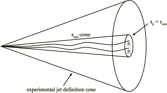
Figure 2: Two unresolved partons according to a physical jet definition (outer cone). Infrared and collinear divergencies in the jet definition cone are isolated by a theoretical “cone” defined by the resolution parameter $s_{\mbox{\scriptsize min}}$.

Infrared as well as collinear divergencies associated with two partons within this jet definition “cone” are further isolated by introducing a purely theoretical parton resolution parameter $s_{\mbox{\scriptsize min}}$ (shown by the inner cone in Fig. 2).

Soft and collinear approximations to the $(n+1)$-final state parton matrix elements are used in the phase space region inside the $s_{\mbox{\scriptsize min}}$ cone, where at least one pair of partons, including initial ones, has $s_{ij}=2p_{i}.p_{j}<s_{\mbox{\scriptsize min}}$. The soft and/or collinear final state parton is then integrated over analytically. Factorizing the collinear initial state divergencies into the bare parton distribution functions and adding this soft+collinear part to the virtual contributions for the $n$-parton final state gives a finite result for, effectively, $n$-parton final states. In general this $n$-parton contribution is negative and grows logarithmically in magnitude as $s_{\mbox{\scriptsize min}}$ is decreased. This logarithmic growth is exactly cancelled by the increase in the $n+1$ parton cross section with $s_{ij}>s_{\mbox{\scriptsize min}}$ (i.e. the region between the two cones in Fig. 2), once $s_{\mbox{\scriptsize min}}$ is small enough for the approximations made within the $s_{\mbox{\scriptsize min}}$-cone to be valid. The integration over the $n+1$-parton phase space with $s_{ij}>s_{\mbox{\scriptsize min}}$ is done by Monte-Carlo techniques in mepjet without using any approximations. Since, at each phase space point, the parton 4-momenta are available, the program is flexible enough to implement any jet definition algorithms or to impose arbitrary kinematical resolution and acceptance cuts on the final state particles [8].

As mentioned before the collinear initial state divergencies are factorized into the bare parton densities introducing a dependence on the factorization scale $\mu_{F}$. In order to handle these singularities we follow Ref. [9] and use the technique of universal “crossing functions” (see section 2.2.4) for the definition and details. The idea is to start with the result of the NLO calculation with all partons in the final state, i.e. $e^{+}e^{-}\rightarrow n+1$ “jets”, where no such singularities occur after adding real and virtual contributions. This NLO $e^{+}e^{-}\rightarrow n+1$ “jets” cross section needs only been known in the soft and collinear limit, where the $e^{+}e^{-}\rightarrow n+2$ parton matrix elements have been integrated analytically over the unresolved region, where one pair of partons has $s_{ij}<s_{\mbox{\scriptsize min}}$. Let us now specify the general structure of the NLO jet cross sections in DIS within the framework of the phase space slicing and the crossing function technique in full detail.

2.2 The General Structure of the NLO Jet Cross Section:
Crossing Functions and Phase Space Slicing Technique

According to the general discussion in the previous section the structure of the $n$-jet cross section up to NLO can be summarized as:

$$\sigma_{\mbox{\scriptsize had}}^{\mbox{\scriptsize NLO}}[n\mbox{-jet}] = \sigma_{\mbox{\scriptsize had}}^{\mbox{\scriptsize LO}}[n\mbox{-jet}]$$

$$+ \sigma_{\mbox{\scriptsize had}}^{\mbox{\scriptsize NLO, virtual+soft+collinear}}[n\mbox{-jet}]$$

$$+ \sigma_{\mbox{\scriptsize had}}^{\mbox{\scriptsize NLO, hard}}[n\mbox{-jet}]$$

where the virtual + soft + collinear piece is given by

$$\sigma_{\mbox{\scriptsize had}}^{\mbox{\scriptsize NLO, virtual+soft+collinear}} = \sigma_{\mbox{\scriptsize had}}^{\mbox{\scriptsize NLO, final}}$$ (7)

$$+ \sigma_{\mbox{\scriptsize had}}^{\mbox{\scriptsize NLO, crossing}}$$

We will now specify the individual pieces in Eqs. (2.2,7) for $n$-jet production in DIS in detail.

2.2.1 The LO Part $\sigma_{\mbox{\scriptsize had}}^{\mbox{\scriptsize LO}}$[$n$-jet]

At LO each jet is modelled by a single outgoing parton:

$$\sigma_{\mbox{\scriptsize had}}^{\mbox{\scriptsize LO}}[n\mbox{-jet}] = \sum_{a}\int_{0}^{1}d\eta\int d{\mbox{PS}}^{(l^{\prime}+n)}f_{a}(\eta,\mu_{F})\,\,$$

$$\alpha_{s}^{(n-1)}(\mu_{R})\,\,\hat{\sigma}^{\mbox{\scriptsize LO}}_{a\rightarrow n\,\,\mbox{\scriptsize partons}}(l+p_{0}\rightarrow l^{\prime}+p_{1}\ldots p_{n})\,\,J_{n\leftarrow n}(\{p_{i}\})$$

where $a=q,\bar{q},g$ and $d\mbox{PS}^{(l^{\prime}+n)}$ stands for the $n+1$ particle Lorentz-invariant phase-space measure

$$d\mbox{PS}^{(l^{\prime}+n)}=\delta^{4}(p_{0}+l-l^{\prime}-\sum_{i=1}^{n}p_{i})\,2\pi\frac{d^{3}l^{\prime}}{2E^{\prime}}\prod_{i=1}^{n}\frac{d^{3}p_{i}}{(2\pi)^{3}\,2E_{i}}\>.$$ (9)

$\hat{\sigma}^{\mbox{\scriptsize LO}}$ denotes the LO $n$-parton final state differential cross section with $\alpha_{s}$ set to one.

The jet algorithm $J_{n\leftarrow n}$, which yields one if the original final state $n$-parton configuration yields $n$ jets satisfying the experimental cuts can be expressed as a product of a clustering part and an acceptance part (jet momenta are denoted by $k_{i}$ in the following):

$$J_{n\leftarrow n}=J_{n\leftarrow n}^{\mbox{\scriptsize cluster}}(p_{1},\ldots,p_{n}\rightarrow k_{1},\ldots,k_{n})\cdot J_{n\leftarrow n}^{\mbox{\scriptsize accept}}(k_{1},\ldots,k_{n}\rightarrow k_{1},\ldots,k_{n})\>.$$ (10)

$J_{n\leftarrow n}^{\mbox{\scriptsize cluster}}$ evaluates to one if all final state partons are well separated according to a given jet algorithm, and vanishes otherwise:

$$J_{n\leftarrow n}^{\mbox{\scriptsize cluster}}(p_{1},\ldots,p_{n}\rightarrow k_{1},\ldots,k_{n})=\prod_{i<j;\,1}^{n}(1-\Theta_{\mbox{\scriptsize cluster}}(p_{i},p_{j}))\>.$$ (11)

The clustering is defined by the $\Theta_{\mbox{\scriptsize cluster}}$ function,

$$\Theta_{\mbox{\scriptsize cluster}}(p_{i},p_{j})=\left\{\begin{array}[]{ll}1,&p_{i},p_{j}\hskip 28.45274pt\mbox{clustered into one jet,}\\ 0,&\mbox{otherwise}\>.\\ \end{array}\right.$$ (12)

The jet momenta $k_{i}$ are functions of the parton momenta $p_{i}$ defined by the recombination algorithm

$$k_{\mbox{\scriptsize jet}}={p_{i}\otimes p_{j}\otimes\ldots}$$ (13)

or simpler in the $E$ scheme

$$k_{\mbox{\scriptsize jet}}=\sum_{i\in\mbox{\scriptsize jet}}p_{i}$$ (14)

Similarly, $J_{n\leftarrow n}^{\mbox{\scriptsize accept}}$ evaluates to one, if all final state jets with momenta $k_{i}$ (=$p_{i}$ in the LO case) pass all acceptance and detector resolution criteria, for example cuts on the transverse momenta, pseudo-rapidities,$\ldots$

$$J_{n\leftarrow n}^{\mbox{\scriptsize accept}}(k_{1},\ldots,k_{n}\rightarrow k_{1},\ldots,k_{n}) =$$

$$\prod_{i=1}^{n}\,\Theta(p_{T}(k_{i})>p_{T,\mbox{\scriptsize min}})\,\,\prod_{i=1}^{n}\,\Theta(|\eta(k_{i})|<\eta_{\mbox{\scriptsize max}})\,\,\prod_{i=1}^{n}\,\Theta(\ldots)\,\,\ldots$$

2.2.2 The NLO Resolved Part $\sigma_{\mbox{\scriptsize had}}^{\mbox{\scriptsize NLO, hard}}$[$n$-jet]

This part calculates the finite contributions from the real emission outside the soft and collinear region.

$$\sigma_{\mbox{\scriptsize had}}^{\mbox{\scriptsize NLO, hard}}[n\mbox{-jet}] = \sum_{a}\int_{0}^{1}d\eta\,\int\,d{\mbox{PS}}^{(l^{\prime}+n+1)}\,\,f_{a}(\eta,\mu_{F})\,\,$$

$$\alpha_{s}^{n}(\mu_{R})\,\,\hat{\sigma}^{\mbox{\scriptsize LO}}_{a\rightarrow(n+1)\,\,\mbox{\scriptsize partons}}(l+p_{0}\rightarrow l^{\prime}+p_{1}\ldots p_{n+1})\,\,\prod_{i<j;\,0}^{n+1}\Theta(|s_{ij}|-s_{\mbox{\scriptsize min}})\,\,J_{n\leftarrow n+1}(\{p_{i}\})$$

where $d\mbox{PS}^{(l^{\prime}+n+1)}$ stands for the $n+2$ particle phase-space measure

$$d\mbox{PS}^{(l^{\prime}+n+1)}=\delta^{4}(p_{0}+l-l^{\prime}-\sum_{i=1}^{n+1}p_{i})\,2\pi\frac{d^{3}l^{\prime}}{2E^{\prime}}\prod_{i=1}^{n+1}\frac{d^{3}p_{i}}{(2\pi)^{3}\,2E_{i}}$$ (17)

and $\hat{\sigma}^{\mbox{\scriptsize LO}}$ denotes the LO $(n+1)$-parton final state differential cross section with $\alpha_{s}$ set to one. The $(n+1)$-parton final state cross section needs to be integrated over the phase space with $s_{ij}=2p_{i}.p_{j}>s_{\mbox{\scriptsize min}}$ ($i,j\in\{0,\ldots,n+1\},\,i<j$), where only $n$ jets are reconstructed according to a given jet definition scheme. The jet algorithm $J_{n\leftarrow n+1}$ in Eq. (2.2.2) evaluates to one if the $(n+1)$- parton configuration yields $n$ detected jets and vanishs otherwise. More precisely, $J_{n\leftarrow n+1}(\{p_{i}\})$ evaluates to one either if one pair of partons is clustered into one jet and the remaining $(n-1)$ partons are well separated from this jet and pass all acceptance criteria (together with the jet) or all $(n+1)$ partons are resolved but one parton does not pass the acceptance cut:

$$J_{n\leftarrow n+1} = J_{n\leftarrow n+1}^{\mbox{\scriptsize cluster}}(p_{1},\ldots,p_{n+1}\rightarrow k_{1},\ldots,k_{n})\cdot J_{n\leftarrow n}^{\mbox{\scriptsize accept}}(k_{1},\ldots,k_{n}\rightarrow k_{1},\ldots,k_{n})$$

$$+ J_{n+1\leftarrow n+1}^{\mbox{\scriptsize cluster}}(p_{1},\ldots,p_{n+1}\rightarrow k_{1},\ldots,k_{n+1})\cdot J_{n\leftarrow n+1}^{\mbox{\scriptsize accept}}(k_{1},\ldots,k_{n+1}\rightarrow k_{1},\ldots,k_{n})$$

with

$$J_{n\leftarrow n+1}^{\mbox{\scriptsize cluster}}(p_{1},\ldots,p_{n+1}\rightarrow k_{1},\ldots,k_{n}) =$$

$$\sum_{i<j}^{n+1}\Theta_{\mbox{\scriptsize cluster}}(p_{i},p_{j})\prod_{l<k;l\neq i,j;k\neq i,j}(1-\Theta_{\mbox{\scriptsize cluster}}(p_{l},p_{k}))\prod_{l;l\neq i,j}(1-\Theta_{\mbox{\scriptsize cluster}}(p_{l},p_{i}\otimes p_{j}))$$

and

$$J_{n\leftarrow n+1}^{\mbox{\scriptsize accept}}(k_{1},\ldots,k_{n+1}\rightarrow k_{1},\ldots,k_{n}) =$$

$$\sum_{i}^{n+1}\Theta[(p_{T}(k_{i})<p_{T,\mbox{\scriptsize min}})\,\,\,\,\mbox{or}\,\,\,\,(|\eta(k_{i})|>\eta_{\mbox{\scriptsize max}})\cdot\prod_{j\neq i}^{n}\,\Theta(p_{T}(k_{i})>p_{T,\mbox{\scriptsize min}})\Theta(|\eta(k_{i})|<\eta_{\mbox{\scriptsize max}})$$

2.2.3 The NLO Unresolved Parts $\sigma_{\mbox{\scriptsize had}}^{\mbox{\scriptsize NLO, final}}$[$n$-jet] and $\sigma_{\mbox{\scriptsize had}}^{\mbox{\scriptsize NLO, crossing}}$[$n$-jet]

The sum of these two pieces is the virtual+soft+collinear part of the NLO $n$-jet cross section in DIS. The first term summarizes the contributions of the integration over the soft and final state collinear regions combined with the corresponding virtual singularities, where all soft and collinear poles cancel according to the Bloch-Nordsiek [27] and Kinoshita-Lee-Nauenberg [28] theorems. Here, the soft and final state collinear regions (referred to as a final state cluster in the following) are defined by the phase space requirement $s_{ij}=2p_{i}.p_{j}<s_{\mbox{\scriptsize min}}$. Absorbing the ultraviolet divergencies in the virtual corrections (for $n\geq 2$ ) into the bare coupling constant according to the modified minimal subtraction ($\overline{\mbox{MS}}$) renormalization scheme [29] yields a finite result. The corresponding finite NLO partonic cross section can be written in the form

$$\alpha_{s}^{n}(\mu_{R})\hat{\sigma}^{\mbox{\scriptsize NLO}}_{a\rightarrow n\,\,\mbox{\scriptsize partons}} \sim$$

$$\alpha_{s}^{n}(\mu_{R})\left[|M^{\mbox{\scriptsize LO}}_{a\rightarrow n\,\,\mbox{\scriptsize partons}}|^{2}\,{\cal{K}}_{a\rightarrow n\,\,\mbox{\scriptsize partons}}(s_{\mbox{\scriptsize min}},s_{ij},\mu_{R})\,+\,{{\cal{F}}_{a\rightarrow n\,\,\mbox{\scriptsize partons}}}\right]$$

where $|M^{\mbox{\scriptsize LO}}_{a\rightarrow n\,\,\mbox{\scriptsize partons}}|^{2}$ denotes the LO matrix element squared with $\alpha_{s}^{(n-1)}$ set to one. The dynamical ${\cal{K}}-$factor, which multiplies the LO matrix element squared depends on the resolution parameter $s_{\mbox{\scriptsize min}}$, the invariant masses of the hard partons and (for $n\geq 2$) on the renormalization scale $\mu_{R}$. The function ${\cal{F}}$ in Eq. (2.2.3) denotes the finite part of the virtual corrections, which does not factorize the Born term amplitude. Both functions ${\cal{K}}_{a\rightarrow n\,\,\mbox{\scriptsize partons}}$ and ${\cal{F}}_{a\rightarrow n\,\,\mbox{\scriptsize partons}}$ can be obtained from the NLO $e^{+}e^{-}\rightarrow(n+1)$ partons result as presented in [6]. The hadronic cross section for the virtual + soft + final state collinear divergencies is thus given by

$$\sigma_{\mbox{\scriptsize had}}^{\mbox{\scriptsize NLO, final}}[n\mbox{-jet}] = \sum_{a}\int_{0}^{1}d\eta\,\int\,d{\mbox{PS}}^{(l^{\prime}+n)}\,\,f_{a}(\eta,\mu_{F})\,\,$$ (22)

$$\alpha_{s}^{n}(\mu_{R})\,\,\hat{\sigma}^{\mbox{\scriptsize NLO}}_{a\rightarrow n\,\,\mbox{\scriptsize partons}}(l+p_{0}\rightarrow l^{\prime}+p_{1}\ldots p_{n};s_{\mbox{\scriptsize min}},\mu_{R})\,\,J_{n\leftarrow n}(\{p_{i}\})$$

where $\alpha_{s}^{n}$ is set to one in the partonic NLO cross section. The crossing of a final state cluster to the initial state, which is effectively done by crossing the function ${\cal{K}}_{a\rightarrow n\,\,\mbox{\scriptsize partons}}$ in Eq. (2.2.3) from the corresponding $e^{+}e^{-}$ results, becomes possible through the introduction of the crossing functions $C_{a}$ [9], which essentially contain the convolution of the parton distribution function with the Altarelli-Parisi kernels. They also take into account the difference between the initial state collinear cluster and the final state collinear cluster together with the factorization of the initial state mass singularities. In the case of DIS the crossing function contribution $\sigma_{\mbox{\scriptsize had}}^{\mbox{\scriptsize NLO, crossing}}$ has the form:

$$\sigma_{\mbox{\scriptsize had}}^{\mbox{\scriptsize NLO, crossing}}[n\mbox{-jet}] = \sum_{a}\int_{0}^{1}d\eta\,\int\,d{\mbox{PS}}^{(l^{\prime}+n)}\,\,\alpha_{s}(\mu_{R})\,\,C_{a}(\eta,\mu_{F},s_{\mbox{\scriptsize min}})\,\,$$ (23)

$$\alpha_{s}^{n-1}(\mu_{R})\,\,\hat{\sigma}^{\mbox{\scriptsize LO}}_{a\rightarrow n\,\,\mbox{\scriptsize partons}}(l+p_{0}\rightarrow l^{\prime}+p_{1}\ldots,p_{n})\,\,J_{n\leftarrow n}(\{p_{i}\})$$

The explicit dependence on the factorization scale $\mu_{F}$ is effectively introduced by the crossing functions $C_{a}(\eta,\mu_{F})$. $J_{n\leftarrow n}(\{p_{i}\})$ in Eqs. (22, 23) represents again the jet algorithm and cuts as in Eq. (2.2.1) for the LO case.

2.2.4 Crossing Functions (Unpolarized Case)

Consider the case where an initial parton $p$ splits into an (unobserved) collinear parton $u$ with momentum $p_{u}=(1-z)p_{p}$ and a parton $a$ with $p_{a}=zp_{p}$ (which participates in the hard scattering): $p\rightarrow ua$. The region where parton $u$ is collinear with $p$ is defined by the invariant mass criterion $|s_{pu}|<s_{\mbox{\scriptsize min}}$. This configuration is indistinguishable from the leading order configuration where parton $a$ comes directly from the proton. After removing the mass singularity at $|s_{pu}|\rightarrow 0$ by mass factorization into the “bare” parton densities the remaining part of the initial state collinear radiation in the phase space region $|s_{pu}|<s_{\mbox{\scriptsize min}}$ is absorbed into effective parton distribution functions, called crossing functions $C_{a}(x,\mu_{F},s_{\mbox{\scriptsize min}})$ [9]. This part of the crossing function is essentially a convolution of the parton densities with the Altarelli-Parisi splitting functions $P_{p\rightarrow a}(z)$ and depends on $s_{\mbox{\scriptsize min}}$, the factorization scale $\mu_{F}$ and on the factorization scheme.

A second contribution to the crossing functions arises from the crossing of a pair of collinear partons $u$ and $p$ (which originates from the splitting $a\rightarrow up$) from the final state to the initial state, which is done in the functions ${\cal{K}}_{a\rightarrow n\,\,\mbox{\scriptsize partons}}$ in Eqs. (2.2.3,22). The crossed pair of collinear final state partons $up$ has been integrated over the final state collinear phase space region defined by the invariant mass criterion $s_{up}<s_{\mbox{\scriptsize min}}$. This “wrong” contribution, which also depends on $s_{\mbox{\scriptsize min}}$, can effectively be subtracted from the parton densities. In fact, the crossing of the final state collinear pair of partons $a\rightarrow up$ to the initial state corresponds to a two parton incoming state with invariant mass smaller than $s_{\mbox{\scriptsize min}}$, which cannot be distinguished from a single incoming parton $a$. The relevant subtraction from the parton distribution function $f_{a}(x,\mu_{F})$ has been performed in the corresponding crossing function $C_{a}(x,\mu_{F},s_{\mbox{\scriptsize min}})$ for the initial state parton $a$.

The crossing functions for an initial state parton $a$, which participates in the hard scattering process, can then be written in the form (for a detailed derivation of the unpolarized crossing functions we refer the reader to [9]):

$$C_{a}^{\overline{\mbox{\scriptsize MS}}}(x,\mu_{F},s_{\mbox{\scriptsize min}})=\left(\frac{N}{2\pi}\right)\left[A_{a}(x,\mu_{F})\ln\left(s_{\mbox{\scriptsize min}}/\mu_{F}\right)+B_{a}^{\overline{\mbox{\scriptsize MS}}}(x,\mu_{F})\right]$$ (24)

with

$$A_{a}(x,\mu_{F})=\sum_{p}A_{p\rightarrow a}(x,\mu_{F})$$ (25)

$$B_{a}^{{\overline{\mbox{\scriptsize MS}}}}(x,\mu_{F})=\sum_{p}B_{p\rightarrow a}^{{\overline{\mbox{\scriptsize MS}}}}(x,\mu_{F})$$ (26)

$N$ denotes the number of colors. The sum runs over $p=q,\bar{q},g$. To be more specific, the crossing functions for valence quarks, for example $u_{v}$ quarks reads:

$$C_{u_{v}}^{\overline{\mbox{\scriptsize MS}}}(x,\mu_{F},s_{\mbox{\scriptsize min}})=\left(\frac{N}{2\pi}\right)\bigg{[}A_{u_{v}\rightarrow u_{v}}(x,\mu_{F})\ln\left(\frac{s_{\mbox{\scriptsize min}}}{\mu_{F}}\right)+B_{u_{v}\rightarrow u_{v}}^{\overline{\mbox{\scriptsize MS}}}(x,\mu_{F})\bigg{]}$$ (27)

For sea quarks, for example $s$ quarks:

$$C_{s}^{\overline{\mbox{\scriptsize MS}}}(x,\mu_{F},s_{\mbox{\scriptsize min}}) = \left(\frac{N}{2\pi}\right)\bigg{[}\bigg{(}A_{s\rightarrow s}(x,\mu_{F})+A_{g\rightarrow s}(x,\mu_{F})\bigg{)}\ln\left(\frac{s_{\mbox{\scriptsize min}}}{\mu_{F}}\right)$$

$$\hskip 56.9055pt+\left(B_{s\rightarrow s}^{\overline{\mbox{\scriptsize MS}}}(x,\mu_{F})+B_{g\rightarrow s}^{\overline{\mbox{\scriptsize MS}}}(x,\mu_{F})\right)\bigg{]}$$

For gluons

$$C_{g}^{\overline{\mbox{\scriptsize MS}}}(x,\mu_{F},s_{\mbox{\scriptsize min}}) = \left(\frac{N}{2\pi}\right)\bigg{[}\bigg{(}A_{g\rightarrow g}(x,\mu_{F})+\sum_{i=q,\bar{q}}A_{i\rightarrow g}(x,\mu_{F})\bigg{)}\ln\left(\frac{s_{\mbox{\scriptsize min}}}{\mu_{F}}\right)$$

$$\hskip 56.9055pt+\bigg{(}B_{g\rightarrow g}^{\overline{\mbox{\scriptsize MS}}}(x,\mu_{F})+\sum_{i=q,\bar{q}}B_{i\rightarrow g}^{\overline{\mbox{\scriptsize MS}}}(x,\mu_{F})\bigg{)}\bigg{]}$$

where the sum $\sum_{i=q,\bar{q}}$ in Eq. (2.2.4) runs over all $n_{f}$ quark (valence and sea) and antiquark flavors. The functions $A_{p\rightarrow a}$ and $B_{p\rightarrow a}^{{\overline{\mbox{\scriptsize MS}}}}$ are defined via a one dimensional integration over the parton densities $f_{p}$, which also involves the integration over $()_{+}$ prescriptions. We have performed this numerical integration in a separate program, which is provided together with the mepjet program, and the results for $A_{p\rightarrow a}$ and $B_{p\rightarrow a}^{{\overline{\mbox{\scriptsize MS}}}}$ for different values of $x$ and $\mu_{F}$ are stored in an array in complete analogy to the usual parton densities, e.g. in Ref. [30]. The finite scheme independent functions $A_{p\rightarrow a}(x,\mu_{F})$ are:

$$A_{g\rightarrow g} = \int_{x}^{1}\frac{dz}{z}\,\,f_{g}(x/z,\mu_{F})\left\{\frac{(11N-2n_{f})}{6N}\delta(1-z)\right.$$ (30)

$$\left.\hskip 56.9055pt\,+\,2\left(\frac{z}{(1-z)_{+}}+\frac{(1-z)}{z}+z(1-z)\right)\right\}$$

$$A_{q\rightarrow q} = \int_{x}^{1}\frac{dz}{z}\,\,f_{q}(x/z,\mu_{F})\frac{2C_{F}}{3}\,\left\{\frac{3}{4}\delta(1-z)\,+\,\frac{1}{2}\left(\frac{1+z^{2}}{(1-z)_{+}}\right)\right\}$$ (31)

$$A_{g\rightarrow q} = \int_{x}^{1}\frac{dz}{z}\,\,f_{g}(x/z,\mu_{F})\,\,\,\frac{1}{4}\,\,\,\hat{P}^{(4)}_{g\rightarrow q}(z)$$ (32)

$$A_{q\rightarrow g} = \int_{x}^{1}\frac{dz}{z}\,\,f_{q}(x/z,\mu_{F})\,\,\,\frac{1}{4}\,\,\,\hat{P}^{(4)}_{q\rightarrow g}(z)$$ (33)

and the scheme dependent functions $B_{p\rightarrow h}^{{\overline{\mbox{\scriptsize MS}}}}(x,\mu_{F})$ by

$$B_{g\rightarrow g}^{{\overline{\mbox{\scriptsize MS}}}} = \int_{x}^{1}\frac{dz}{z}\,\,f_{g}(x/z,\mu_{F})\left\{\left(\frac{\pi^{2}}{3}-\frac{67}{18}+\frac{5n_{f}}{9N}\right)\delta(1-z)+2z\left(\frac{\ln(1-z)}{(1-z)}\right)_{+}\right.$$ (34)

$$\hskip 99.58464pt\left.+2\left(\frac{(1-z)}{z}+z(1-z)\right)\ln(1-z)\right\}$$

$$B_{q\rightarrow q}^{{\overline{\mbox{\scriptsize MS}}}} = \int_{x}^{1}\frac{dz}{z}\,\,f_{q}(x/z,\mu_{F})\frac{2C_{F}}{3}\,\left\{\left(\frac{\pi^{2}}{6}-\frac{7}{4}\right)\delta(1-z)+\frac{1}{2}(1-z)\right.$$ (35)

$$\hskip 99.58464pt\left.+\frac{1}{2}(1+z^{2})\left(\frac{\ln(1-z)}{(1-z)}\right)_{+}\right\}$$

$$B_{g\rightarrow q}^{{\overline{\mbox{\scriptsize MS}}}} = \int_{x}^{1}\frac{dz}{z}\,\,f_{g}(x/z,\mu_{F})\,\,\,\frac{1}{4}\,\,\,\left\{\hat{P}^{(4)}_{g\rightarrow q}(z)\ln(1-z)-\hat{P}^{(\epsilon)}_{g\rightarrow q}(z)\right\}$$ (36)

$$B_{q\rightarrow g}^{{\overline{\mbox{\scriptsize MS}}}} = \int_{x}^{1}\frac{dz}{z}\,\,f_{q}(x/z,\mu_{F})\,\,\,\frac{1}{4}\,\,\,\left\{\hat{P}^{(4)}_{q\rightarrow g}(z)\ln(1-z)-\hat{P}^{(\epsilon)}_{q\rightarrow g}(z)\right\}$$ (37)

where $n_{f}$ is Eqs. (30,34) denotes the number of flavors and $N=3$ is the number of colors. The Altarelli-Parisi kernels in the previous equations are

$$\hat{P}^{(n\neq 4)}_{g\rightarrow g}(z) = {P}^{(n\neq 4)}_{g\rightarrow g}(z)\,\,\,\,=\,4\,\left(\frac{z}{1-z}+\frac{1-z}{z}+z(1-z)\right)$$ (38)

$$\hat{P}^{(n\neq 4)}_{q\rightarrow g}(z) = \frac{8}{9}{P}^{(n\neq 4)}_{q\rightarrow g}(z)=\frac{16}{9}\left(\frac{1+(1-z)^{2}}{z}-\epsilon z\right)$$ (39)

$$\hat{P}^{(n\neq 4)}_{g\rightarrow q}(z) = \frac{1}{3}P^{(n\neq 4)}_{g\rightarrow q}(z)=\frac{2}{3}\,\left(\frac{z^{2}+(1-z)^{2}-\epsilon}{1-\epsilon}\right)$$ (40)

$$\hat{P}^{(n\neq 4)}_{q\rightarrow q}(z) = \frac{8}{9}P^{(n\neq 4)}_{q\rightarrow q}(z)=\frac{16}{9}\left(\frac{1+z^{2}}{1-z}-\epsilon(1-z)\right)$$ (41)

where $P_{ij}^{(\epsilon)}$ is the $\epsilon$ dimensional part of these $n-$dimensional splitting functions

$$\hat{P}^{(\epsilon)}_{q\rightarrow g}(z) = \frac{8}{9}{P}^{(\epsilon)}_{q\rightarrow g}(z)=-\frac{8}{9}\,2z$$ (42)

$$\hat{P}^{(\epsilon)}_{g\rightarrow q}(z) = \frac{1}{3}P^{(\epsilon)}_{g\rightarrow q}(z)=-\frac{4}{3}\,z(1-z)$$ (43)

The $(\,\,\,)_{+}$ prescriptions in Eqs. (30,31,34,35) are defined for an arbitrary test function $g(z)$ (which is well behaved at $z=1$) as

$$\int_{x}^{1}dz\frac{g(z)}{(1-z)_{+}} = \int_{x}^{1}dz\frac{g(z)-g(1)}{1-z}\,+\,g(1)\log(1-x)$$ (44)

$$\int_{x}^{1}dzg(z)\left(\frac{\log(1-z)}{1-z}\right)_{+} = \int_{x}^{1}dz\frac{g(z)-g(1)}{1-z}\,+\,\frac{1}{2}g(1)\log^{2}(1-x)$$ (45)

The structure and use of the crossing functions are completely analog to the usual parton distribution function. Explicit examples of their appearance and use in NLO 1-jet and 2-jet cross section in DIS are given in Eqs. (4.1.4,5.2.4). Note that a set of crossing functions $C_{a}(\eta,\mu_{F},s_{\mbox{\scriptsize min}})$ has to be calculated (using an extra program provided together with mepjet) for each chosen set of parton distribution functions $f_{a}(\eta,\mu_{F})$ in a NLO calculation.

3 Jet Definitions in DIS

Jet studies on the experimental (hadronic) and theoretical (partonic) level require an exact definition of resolvable jets. The definition of resolvable jets is given by a jet algorithm which organizes the sprays of hadrons (or partons) in an event into a small number of jets. Such a jet algorithm is usually defined in terms of one or more resolution parameters, and a description of how to combine cluster of particles or jets which do not fulfill the resolution criteria. By identifying high transverse momentum clusters on the experimental and theoretical level w.r.t. the proton direction in both the lab and Breit (or HCM) frame one can make a connection with the underlying primordial partonic scattering and apply perturbative QCD for the theoretical prediction. Therefore, jet production provides an intuitive test of the underlying parton structure of hadronic events. Clearly, all jet definition schemes have to be infrared and collinear safe, or in other words the resulting jet cross sections are not affected when an infinitely soft parton is added or when a massless parton is replaced by a collinear pair of massless partons. Preferred jet algorithms are those with small higher-order corrections, small hadronization corrections, and small recombination scheme dependences.

Jet algorithms are represented by “$\theta$-functions” in this paper, denoted by $J_{n\leftarrow n}$ for LO (see Eq. (10)) and $J_{n\leftarrow n+1}$ for NLO (see Eq. (2.2.2)) calculations, which can be expressed as a product of a resolution/clustering part and an acceptance part. For the appearance of these jet-algorithms in NLO calculations see Eqs. (4.1.4,5.2.4,8.2).

Jet definitions in DIS are applied in the laboratory frame at HERA (defined by the 27.5 GeV lepton and the 820 GeV proton beam), in the hadronic center of mass (HCM) frame (=the virtual boson and proton rest frame) and the Breit frame. The Breit frame is characterized by the vanishing energy component of the momentum of the exchanged virtual boson, i.e. the momentum transfer $q$ is purely spacelike. Both the boson momentum

$$q=(0,0,0,-2xE),\,\hskip 28.45274pt\,\,-q^{2}=Q^{2}=4x^{2}E^{2}$$ (46)

and the proton momentum

$$P=E(1,0,0,1)=\frac{Q}{2x}(1,0,0,-1)$$ (47)

are chosen along the $z$-direction. Here, $x$ is the standard Bjorken scaling variable. Unless stated otherwise and in all frames, the proton direction defines the $+z$ direction in this paper.

The following jet algorithms have been used in DIS:

• $W$-scheme:
  In the $W$-scheme, which was introduced for DIS in Refs. [11, 5] in analogy to the JADE scheme for $e^{+}e^{-}$ [31], the invariant mass squared, $s_{ij}=(p_{i}+p_{j})^{2}$, is calculated for each pair of final state particles (including the proton remnant). If the pair with the smallest invariant mass squared is below $y_{cut}W^{2}$, the pair is clustered according to a recombination scheme (see below). This process is repeated until all invariant masses are above $y_{cut}W^{2}$.

• JADE-scheme:
  The experimental analyses in [32] are based on a variant of the $W$-scheme, the “JADE” algorithm [31]. It is obtained from the $W$-scheme by replacing the invariant definition $s_{ij}=(p_{i}+p_{j})^{2}$ by $M_{ij}^{2}=2E_{i}E_{j}(1-\cos\theta_{ij})$, where all quantities are defined in the laboratory frame. At LO the $W$ and the JADE scheme are equivalent. However, neglecting the explicit mass terms $p_{i}^{2}$ and $p_{j}^{2}$ in the definition of $M_{ij}^{2}$ causes substantial differences in NLO dijet cross sections between the $W$ and the JADE scheme. The NLO cross sections in the two schemes can differ dramatically [2, 3] (see section 5.3.3). One problem with the JADE- or $W$-scheme is that the resulting jets can still have very low transverse momenta (see for example Fig. 20b in section 5.3.3). We recomment therefore to impose additional cuts on the jet transverse momenta after the clustering in these schemes.

• cone schemes:
  In the cone algorithm (which can be defined in the laboratory frame, the HCM or the Breit frame) the distance $\Delta R=\sqrt{(\Delta\eta)^{2}+(\Delta\phi)^{2}}$ between two partons decides whether they should be recombined according to a given recombination scheme (see below) to a single jet. Here the variables are the pseudo-rapidity $\eta$ and the azimuthal angle $\phi$. Applicability of fixed order perturbation theory requires sufficiently high transverse momenta of the jets in both the lab and Breit frame. Since the initial state collinear singularity in DIS is restricted to the proton remnant direction, a minimal transverse momentum requirement on the jets can alternatively be replaced by an effective transverse momentum cut for the forward direction, i.e. a $k_{T,{\mbox{\scriptsize min}}}^{B}(j)$ cut, where $k_{T}^{B}(j)$ is defined in Eq. (126).

• $k_{T}$ scheme:
  For the $k_{T}$ algorithm (which is implemented in the Breit frame), we follow the description introduced in Ref. [33].

  After defining a hard scattering scale $E_{T}$ and a particle resolution parameter $y_{cut}$ the following quanities are calculated:

  $$d_{kP}=2\min(E_{i}^{2},E_{P}^{2})(1-\cos\theta_{iP})$$ (48)

  (the “transverse energy” of particle $k$ with respect to the incoming proton) where the subscripts $k$ and $P$ denote the final particle and proton, respectively, and

  $$d_{ij}=2\min(E_{i}^{2},E_{j}^{2})(1-\cos\theta_{ij})$$ (49)

  (the “transverse energy” of particle $i$ with respect to particle $j$). If $d_{kP}<d_{ij}$ and $d_{kP}<E_{T}^{2}$, then particle $k$ is eliminated from further clustering considerations and is associated with the proton remnant. If $d_{ij}<d_{kP}$ amd $d_{ij}<E_{T}^{2}$, particle $i$ and $j$ are recombined into a single pre-cluster (or “macro jet”) according to a recombination prescription. This iteration continues for all particles and pre-clusters until all objects have been formed into single pre-clusters or included into the proton remnant. For $y_{cut}=1$ these final objects are the final jets. The single pre-clusters can be further resolved if $y_{cut}<1$. If any pair $k$ and $l$ in a pre cluster has $d_{kl}<y_{cut}E_{T}^{2}$, these particles are further combined into a single jet until all objects in a pre-cluster have $d_{kl}>y_{cut}E_{T}^{2}$.

Various other definitions could be chosen as for example the “mixed scheme” in Ref. [11] or the ARCLUS algorithm proposed in Ref. [34].

On top of these jet resolution criteria, several prescriptions of how to combine a cluster of particles which do not fulfill the resolution criteria have been used, i.e. how the momenta of partons (or hadrons/cluster of particles) are recombined to give a composite momentum in this case. The recombined momentum is denoted by $p^{\mu}_{rec}=(E_{rec},\vec{p}_{rec})$ with $E_{rec}=\alpha\,\,(E_{1}+E_{2})$ and $\vec{p}_{rec}=\beta\,\,(\vec{p}_{1}+\vec{p}_{2}).$ The energy and momentum rescaling factors $\alpha$ and $\beta$ define the $E$-scheme, $E0$-scheme and $P$-scheme as follows [35]:

$$\begin{array}[]{lll}E-\mbox{scheme}:&\alpha=1&\beta=1\\ E0-\mbox{scheme}:&\alpha=1&\beta=\frac{E_{1}+E_{2}}{|\vec{p_{1}}+\vec{p}_{2}|}\\ P-\mbox{scheme}:&\alpha=\frac{|\vec{p_{1}}+\vec{p}_{2}|}{E_{1}+E_{2}}&\beta=1\\ \end{array}$$ (50)

Obviously, the $E$ scheme conserves energy-momentum, while the $E0$ ($P$) scheme conserves only energy (momentum). The rescaling factors for the $E0$ and $P$ scheme are chosen such that the recombined four-vector has zero mass. The recombined vector is only in the $E$ scheme not massless.

Another commonly used recombination scheme for jets defined in a cone scheme has been proposed in Ref. [36]. Here, the transverse energy, pseudo-rapidity and azimuthal angle of the jets are calculated by performing energy weighted sums over the particles within the cone radius $R$,

$$E_{T} = \sum_{i\in R}E_{Ti}$$

$$\eta_{\mbox{\scriptsize jet}} = \frac{1}{E_{T}}\sum_{i\in R}E_{Ti}\,\,\eta_{i}$$ (51)

$$\phi_{\mbox{\scriptsize jet}} = \frac{1}{E_{T}}\sum_{i\in R}E_{Ti}\,\,\phi_{i}$$

Several variants of Eq. (51) have been used for the cone scheme in hadron hadron collisions: the “fixed-cone” algorithm used by UA2 [37], the “iterative-cone” algorithm used by both CDF and D0 collaborations at the FERMILAB collider [38, 39], the “EKS” algorithm introduced in Ref. [40]. For a recent discussion of various definitions, including a detailed discussion of problems related to overlapping cones, we refer the reader to [41, 42].

It is clear that the algorithms (including the recombination prescriptions) in the theoretical calculations must be matched to the chosen experimental definition. Unless stated otherwise, and for all jet algorithms, we use the $E$-scheme to recombine partons, i.e. the cluster momentum is taken as $p_{i}+p_{j}$, the sum of the 4-momenta of partons $i$ and $j$, if these are unresolved according to a given jet definition scheme. Large recombination scheme dependencies have been found in particular for the $W$ scheme [2] (see also section 5.3.3).

4 One-Jet Cross Sections

4.1 NLO One-Jet and Total ${\cal{O}}({\boldmath{\alpha_{s}}})$ Cross Sections
(One-Photon Exchange)

The 1-jet final state is the most basic high transverse momentum event at HERA, with a lepton and a jet back-to-back in the transverse plane. The lowest order ${\cal{O}}(\mbox{$\alpha_{s}$}^{0})$ partonic contribution to the 1-jet cross section arises from the quark parton model (QPM) subprocess (see Fig. 3a)

$$e(l)+q(p_{0})\rightarrow e(l^{\prime})+q(p_{1})$$ (52)

and the corresponding anti-quark process with $q\leftrightarrow\bar{q}$. Imposing no (or sufficiently weak cuts on the scattered parton) yields directly the total DIS cross section in the parton model.

Figure 3: Zeroth order Born diagram (a) for lepton parton scattering and virtual gluon corrections (b) to the Born process.

The NLO ${\cal{O}}(\mbox{$\alpha_{s}$})$ 1-jet cross section receives contributions from the 1-loop corrections to the subprocess in Eq. (52) (see Fig. 3b) and from the 2-parton tree level final state matrix elements (see Fig. 4)

$$e(l)+q(p_{0}) \rightarrow e(l^{\prime})+q(p_{1})+g(p_{2})$$ (53)

$$e(l)+g(p_{0}) \rightarrow e(l^{\prime})+q(p_{1})+\bar{q}(p_{2})$$ (54)

and the corresponding anti-quark processes with $q\leftrightarrow\bar{q}$.

Figure 4: First order $\mbox{$\cal{O}$}(\alpha_{s})$ tree graph two parton final state processes: quark initiated “Compton process” (a) and boson-gluon fusion process (b).

According to Eqs. (2.2,7) the NLO 1-jet exclusive cross section is given by

$$\sigma_{\mbox{\scriptsize had}}^{\mbox{\scriptsize NLO}}[1\mbox{-jet}] = \sigma_{\mbox{\scriptsize had}}^{\mbox{\scriptsize LO}}[1\mbox{-jet}]$$

$$+ \sigma_{\mbox{\scriptsize had}}^{\mbox{\scriptsize NLO, final}}[1\mbox{-jet}]$$

$$+ \sigma_{\mbox{\scriptsize had}}^{\mbox{\scriptsize NLO, crossing}}[1\mbox{-jet}]$$

$$+ \sigma_{\mbox{\scriptsize had}}^{\mbox{\scriptsize NLO, hard}}[1\mbox{-jet}]$$

where the hadronic cross sections on the r.h.s. of Eq. (4.1) are defined in Eqs. (2.2.1,22,23,2.2.2) for $n=1$, respectively. The required partonic cross sections in the hadronic cross sections in Eq. (4.1) will be discussed in the following subsections. The final formula for the hadronic NLO 1-jet exclusive cross section in terms of these partonic results is given in Eq. (4.1.4).

The total $\mbox{$\cal{O}$}(\alpha_{s})$ cross section can be obtained from Eqs. (4.1,4.1.4) by adding the LO two jet cross section, i.e. the total cross section is defined as the NLO 1-jet inclusive cross section, provided the cuts on the jets are sufficiently weak (see section 4.2).

Let us now specify the relevant partonic cross sections for the hadronic cross sections in Eq. (4.1).

4.1.1 $\hat{\sigma}^{\mbox{\scriptsize LO}}_{q\rightarrow q}$ in $\sigma_{\mbox{\scriptsize had}}^{\mbox{\scriptsize LO}}$[1-jet] and $\sigma_{\mbox{\scriptsize had}}^{\mbox{\scriptsize NLO, crossing}}$[1-jet]

According to Eqs. (2.2.1,23) the partonic cross section

$$\hat{\sigma}^{\mbox{\scriptsize LO}}_{q\rightarrow q}=\sigma_{0}\,\,e_{q}^{2}\,\,|M^{(\mbox{\scriptsize pc})}_{q\rightarrow q}|^{2}$$ (56)

for the subprocess in Eq. (52) enters the hadronic cross sections $\sigma_{\mbox{\scriptsize had}}^{\mbox{\scriptsize LO}}$[1-jet] and $\sigma_{\mbox{\scriptsize had}}^{\mbox{\scriptsize NLO, crossing}}$[1-jet] where (a numerical factor $1/4$ for the initial state spin average is included in $\sigma_{0}$)

$$\sigma_{0}=\frac{1}{4p_{0}.l}\,\frac{1}{4}\,\frac{(4\pi\alpha)^{2}}{Q^{4}}$$ (57)

and

$$|M^{(\mbox{\scriptsize pc})}_{q\rightarrow q}|^{2}=32\,\left[(p_{0}.l)^{2}\,+\,(p_{0}.l^{\prime})^{2}\,\right]\,=\,8\hat{s}^{2}\,\,(1+(1-y)^{2})$$ (58)

The superscript (pc) ($\equiv$ parity conserving) refers to the vector current coupling at the leptonic and hadronic vertices and $\hat{s}=\eta s$ denotes the partonic center of mass energy squared.

4.1.2 $\hat{\sigma}^{\mbox{\scriptsize NLO}}_{q\rightarrow q}$ in $\sigma_{\mbox{\scriptsize had}}^{\mbox{\scriptsize NLO, final}}$[1-jet]

According to Eq. (2.2.3) the NLO (finite) partonic cross section

$$\mbox{$\alpha_{s}$}\,\hat{\sigma}^{\mbox{\scriptsize NLO}}_{q\rightarrow q}\,\,=\alpha_{s}\,\,\sigma_{0}\,\,e_{q}^{2}\,\,\left[|M^{(\mbox{\scriptsize pc})}_{q\rightarrow q}|^{2}\,\,{\cal{K}}_{q\rightarrow q}(s_{\mbox{\scriptsize min}},Q^{2})+{\cal{F}}_{q\rightarrow q}\right]$$ (59)

in the hadronic cross section $\sigma_{\mbox{\scriptsize had}}^{\mbox{\scriptsize NLO, final}}$[1-jet] combines the virtual 1-loop corrections in Fig. 3b to the Born process in Eq. (52) with the singular integrals over the two parton final state unresolved phase space region for the subprocesses in Eqs. (53) and (54) (see Fig. 4). All finite parts of the virtual corrections factorize the Born matrix element in the 1-jet case and hence ${\cal{F}}_{q\rightarrow q}$ in Eq. (59) vanishes. The dynamical ${\cal{K}}_{q\rightarrow q}$ factor, which multiplies the lowest order ${\cal{O}}(\alpha_{s}^{0})$ matrix element squared, depends on both $s_{\mbox{\scriptsize min}}$ and the invariant mass of the hard partons $2p_{0}.p_{1}=Q^{2}$ ($N=3$ is the number of colors):

$${\cal{K}}_{q\rightarrow q}(s_{\mbox{\scriptsize min}},Q^{2})=\frac{8}{9}\,\left(\frac{N}{2\pi}\right)\left[-\ln^{2}\left(\frac{s_{\mbox{\scriptsize min}}}{Q^{2}}\right)-\frac{3}{2}\ln\left(\frac{s_{\mbox{\scriptsize min}}}{Q^{2}}\right)-\frac{\pi^{2}}{3}-\frac{1}{2}\,+\,{\cal{O}}(s_{\mbox{\scriptsize min}})\right]$$ (60)

Terms proportional to $s_{\mbox{\scriptsize min}}$ have been neglected in Eq. (60). ${\cal{K}}_{q\rightarrow q}$ may be crossed in exactly the same manner as the usual tree level crossing from the ${\cal{K}}$ factor in $e^{+}e^{-}\rightarrow$ 2 partons as given in Eq. (4.31) with $n=0$ in Ref [6]. Thus, Eq. (60) includes also the crossing of a pair of collinear partons with an invariant mass smaller than $s_{\mbox{\scriptsize min}}$ from the final state to the initial state. This “wrong” contribution is replaced by the correct collinear initial state configuration by adding the appropriate crossing function contribution to the hadronic cross section as given in Eq. (4.1.4). The crossing function contribution in Eq. (4.1.4) takes also into account the corresponding factorization of the initial state singularities, which is encoded in the crossing functions $C_{q}^{\overline{\mbox{\scriptsize MS}}}$ for valence and sea quark distributions as described in Eqs. (27,2.2.4).

4.1.3 $\hat{\sigma}^{\mbox{\scriptsize LO}}_{q\rightarrow qg}$ and $\hat{\sigma}^{\mbox{\scriptsize LO}}_{g\rightarrow q\bar{q}}$ in $\sigma_{\mbox{\scriptsize had}}^{\mbox{\scriptsize NLO, hard}}$[1-jet]

According to Eq. (2.2.2) $\sigma_{\mbox{\scriptsize had}}^{\mbox{\scriptsize NLO, hard}}$[1-jet] calculates the finite contributions from the real emission outside the soft and collinear region $(s_{ij}>s_{\mbox{\scriptsize min}}$) for the 2-parton final state subprocesses in Eqs. (53) and (54) (Fig. 4). The partonic cross sections in 1-photon exchange are:

$$\mbox{$\alpha_{s}$}\,\hat{\sigma}^{\mbox{\scriptsize LO}}_{q\rightarrow qg}\,\, = \sigma_{0}\,\,e_{q}^{2}\,\,(4\pi\alpha_{s}(\mu_{R}))\,\,|M^{(\mbox{\scriptsize pc})}_{q\rightarrow qg}|^{2}$$ (61)

$$\mbox{$\alpha_{s}$}\,\hat{\sigma}^{\mbox{\scriptsize LO}}_{g\rightarrow q\bar{q}}\,\, = \sigma_{0}\,\,e_{q}^{2}\,\,(4\pi\alpha_{s}(\mu_{R}))\,\,|M^{(\mbox{\scriptsize pc})}_{g\rightarrow q\bar{q}}|^{2}$$ (62)

with [see appendix A.2]

$$|M^{(\mbox{\scriptsize pc})}_{q\rightarrow qg}|^{2} = \frac{128}{3}\,\,(l.l^{\prime})\,\,\frac{(l.p_{0})^{2}+(l^{\prime}.p_{0})^{2}+(l.p_{1})^{2}+(l^{\prime}.p_{1})^{2}}{(p_{1}.p_{2})(p_{0}.p_{2})}$$ (63)

$$|M^{(\mbox{\scriptsize pc})}_{g\rightarrow q\bar{q}}|^{2} = -\frac{3}{8}\,\,|M^{(\mbox{\scriptsize pc})}_{q\rightarrow qg}|^{2}(p_{0}\leftrightarrow-p_{2})$$ (64)

$$= 16\,\,(l.l^{\prime})\,\,\frac{(l.p_{2})^{2}+(l^{\prime}.p_{2})^{2}+(l.p_{1})^{2}+(l^{\prime}.p_{1})^{2}}{(p_{0}.p_{1})(p_{0}.p_{2})}$$

Color factors (including the initial state color average) are included in these squared matrix elements. The superscript (pc) refers again to the vector current coupling of the virtual photon at the leptonic and hadronic vertex. Note that the initial state spin average factors are included in the definition of $\sigma_{0}$ in Eq. (58). These compact expressions for the squared matrix elements can be obtained by analytically squaring the helicity amplitudes for the subprocesses in Eqs. (53,54) in the Weyl-van der Waerden formalism as shown in appendix A.2 and therefore, the full spin structure is kept. In fact, each addend in Eqs. (63) and (64) corresponds to a specific helicity configuration for the external particles as listed in table 1.

Table 1: Helicity dependent contributions to the squared matrix elements in Eqs. (63) and (64). The helicities $\lambda_{i}$ are defined via $e(\lambda_{l})q(\lambda_{0})\rightarrow e(\lambda_{l^{\prime}})q(\lambda_{1})g(\lambda_{2})$ and $e(\lambda_{l})g(\lambda_{0})\rightarrow e(\lambda_{l^{\prime}})q(\lambda_{1})\bar{q}(\lambda_{2}).$ The identical contributions from the four nonvanishing remaining helicity combinations with all helicities reversed are not listed in the table (see appendix A.2).

$eq\rightarrow eqg$	$\lambda_{0}$	$\lambda_{1}$	$\lambda_{2}$	$\lambda_{l}$	$\lambda_{l^{\prime}}$		$eg\rightarrow eq\bar{q}$	$\lambda_{0}$	$\lambda_{1}$	$\lambda_{2}$	$\lambda_{l}$	$\lambda_{l^{\prime}}$
$\sim(l.p_{0})^{2}$	$+$	$+$	$+$	$+$	$+$		$\sim(l.p_{2})^{2}$	$-$	$+$	$-$	$+$	$+$
$\sim(l^{\prime}.p_{0})^{2}$	$+$	$+$	$+$	$-$	$-$		$\sim(l^{\prime}.p_{2})^{2}$	$-$	$+$	$-$	$-$	$-$
$\sim(l.p_{1})^{2}$	$-$	$-$	$+$	$+$	$+$		$\sim(l.p_{1})^{2}$	$-$	$-$	$+$	$+$	$+$
$\sim(l^{\prime}.p_{1})^{2}$	$-$	$-$	$+$	$-$	$-$		$\sim(l^{\prime}.p_{1})^{2}$	$-$	$-$	$+$	$-$	$-$

Thus, all lepton-hadron and jet-jet correlations are fully taken into account. The squared matrix elements $|M^{(\mbox{\scriptsize pc})}_{q\rightarrow qg}|^{2}$ and $|M^{(\mbox{\scriptsize pc})}_{g\rightarrow q\bar{q}}|^{2}$ are expressed in terms of more DIS like (partonic) variables in section B.2. The resulting expressions naturally factorize the characteristic $y$ and $\phi$ dependencies for the helicity cross sections $d\sigma^{F_{i}}$ (see Eq. (91)).

Note that the results in Eqs. (63,64) contain the full polarization dependence of the virtual boson, i.e.

These results can also be expressed in terms of helicity cross sections $d\sigma^{F_{i}}$ which correspond to certain polarization states of the exchanged virtual boson (see section 5.1).

4.1.4 The Hadronic One-Jet Cross Section

Based on Eq. (4.1) and the results in the previous sections, the hadronic 1-jet exclusive cross section in the 1-photon exchange up to ${\cal{O}}(\alpha_{s})$ reads
                                                                                                                                           

$$\displaystyle\sigma_{\mbox{\scriptsize had}}[\mbox{1-jet}] =$$

$$\int_{0}^{1}d\eta\int\,d{\mbox{PS}}^{(l^{\prime}+1)}\,\,\sigma_{0}\,\,\bigg{[}$$

$$[\sum_{i=q,\bar{q}}e_{i}^{2}f_{i}(\eta,\mu_{F})\big{]}\,\,\,|M^{(\mbox{\scriptsize pc})}_{q\rightarrow q}|^{2}\,\left(1+\alpha_{s}(\mu_{R})\,{\cal{K}}_{q\rightarrow q}(s_{\mbox{\scriptsize min}},Q^{2})\right)$$

$$+ \,[\sum_{i=q,\bar{q}}e_{i}^{2}\,\,C_{i}^{\overline{\mbox{\scriptsize MS}}}(\eta,\mu_{F},s_{\mbox{\scriptsize min}})]\,\,\alpha_{s}(\mu_{R})\,\,\,|M^{(\mbox{\scriptsize pc})}_{q\rightarrow q}|^{2}\,\,\bigg{]}J_{1\leftarrow 1}(\{p_{i}\})$$

$$+\int_{0}^{1}d\eta\int\,d\mbox{PS}^{(l^{\prime}+2)}\,\,\sigma_{0}\,\,(4\pi\alpha_{s}(\mu_{R}))\,\,\bigg{[}$$

$$[\sum_{i=q,\bar{q}}e_{i}^{2}f_{i}(\eta,\mu_{F})]\,\,\,|M^{(\mbox{\scriptsize pc})}_{q\rightarrow qg}|^{2}$$

$$+ (\sum_{i=q}e_{i}^{2})f_{g}(\eta,\mu_{F})\,\,\,|M^{(\mbox{\scriptsize pc})}_{g\rightarrow q\bar{q}}|^{2}\bigg{]}\,\,\prod_{i<j;\,0}^{2}\Theta(|s_{ij}|-s_{\mbox{\scriptsize min}})\,\,J_{1\leftarrow 2}(\{p_{i}\})$$

where the Lorentz-invariant phase space measure $d\mbox{PS}^{(l^{\prime}+n)}$ is defined in Eq. (9). Analytical expressions for $|M^{(\mbox{\scriptsize pc})}_{q\rightarrow q}|^{2},{\cal{K}}_{q\rightarrow q},|M^{(\mbox{\scriptsize pc})}_{q\rightarrow qg}|^{2}$ and $|M^{(\mbox{\scriptsize pc})}_{g\rightarrow q\bar{q}}|^{2}$ are listed in Eqs. (58,60,63,64), the crossing functions $C_{q}^{\overline{\mbox{\scriptsize MS}}}$ for valence and sea quark distributions in Eqs. (27,2.2.4), and the general structure of the jet algorithms $J_{1\leftarrow 1}(\{p_{i}\})$ and $J_{1\leftarrow 2}(\{p_{i}\})$ is described in Eqs. (10) and (2.2.2), respectively. The 1-jet inclusive cross section is defined via Eq. (4.1.4) by replacing $J_{1\leftarrow 2}(\{p_{i}\})$ in the last line by ($J_{1\leftarrow 2}(\{p_{i}\})+J_{2\leftarrow 2}(\{p_{i}\}))$, i.e. the 1-jet inclusive cross section is defined as the sum of the NLO 1-jet exclusive cross section (as defined in Eq. (4.1.4)) plus the LO two jet cross section.

Eq. (4.1.4) includes all relevant information to construct a Monte Carlo program for the numerical evaluation of the fully differential NLO 1-jet cross section in DIS. In particular all “plus prescriptions” associated with the factorization of the initial state collinear divergencies are absorbed in the crossing functions $C_{q}^{\overline{\mbox{\scriptsize MS}}}$ which is very useful for a Monte Carlo approach.

Note that the second integral over the bremsstrahlung matrix elements is restricted to regions where all partons are resolved, i.e. any pair of partons has $s_{ij}>s_{\mbox{\scriptsize min}}$. As mentioned before, $s_{\mbox{\scriptsize min}}$ is an arbitrary theoretical parameter and any measurable quantity should not depend on it. The bremsstahlung contribution grows with $\ln^{2}s_{\mbox{\scriptsize min}}$ and $\ln s_{\mbox{\scriptsize min}}$ with decreasing $s_{\mbox{\scriptsize min}}$. This logarithmic growth is exactly cancelled by the explicit $-\ln^{2}s_{\mbox{\scriptsize min}}$ and $-\ln s_{\mbox{\scriptsize min}}$ terms in ${\cal{K}}_{q\rightarrow q}(s_{\mbox{\scriptsize min}},Q^{2})$ (see Eq. (60)) and the $s_{\mbox{\scriptsize min}}$ dependence in the the crossing functions $C_{q}^{\overline{\mbox{\scriptsize MS}}}(\eta,\mu_{F},s_{\mbox{\scriptsize min}})$ once $s_{\mbox{\scriptsize min}}$ is small enough for the soft and collinear approximations in ${\cal{K}}_{q\rightarrow q}$ and $C_{q}^{\overline{\mbox{\scriptsize MS}}}$ to be valid. The explicit $s_{\mbox{\scriptsize min}}$ dependence of $C_{q}^{\overline{\mbox{\scriptsize MS}}}$ is discussed in sect. 2.2.4.

A powerful test of the numerical program is the $s_{\mbox{\scriptsize min}}$ independence of the NLO 1-jet cross sections. Fig. 5 shows the inclusive 1-jet cross section for HERA energies as a function of $s_{\mbox{\scriptsize min}}$ for jets defined in a cone scheme (in the laboratory frame) with $\Delta R=1$ for different $Q^{2}$ bins.

Figure 5: Dependence of the inclusive 1-jet cross section in a cone scheme on $s_{\mbox{\scriptsize min}}$, the two-parton resolution parameter, for four $Q^{2}$ bins. Error bars represent statistical errors of the Monte Carlo program. $s_{\mbox{\scriptsize min}}$ independence in the four $Q^{2}$ bins is achieved for $s_{\mbox{\scriptsize min}}\mathrel{\raise 0.86108pt\hbox{$<$}\hskip-8.00003pt\lower 3.87495pt\hbox{$\sim$}}1\,(a),3\,(b),100\,(c),100\,(d)$ GeV².

One observes that for $s_{\mbox{\scriptsize min}}$ values $\mathrel{\raise 0.86108pt\hbox{$<$}\hskip-8.00003pt\lower 3.87495pt\hbox{$\sim$}}$ 1,3,100,100 GeV² the results are indeed independent of $s_{\mbox{\scriptsize min}}$ for the four $Q^{2}$ bins in Fig. 5a,b,c,d, respectively (within one percent, which is about the statistical error in the Monte Carlo runs). Since $Q^{2}$ sets the typical hard scale for 1-jet production, $s_{\mbox{\scriptsize min}}$ independence of the results is indeed expected to start at higher $s_{\mbox{\scriptsize min}}$ values with increasing $Q^{2}$. The $s_{\mbox{\scriptsize min}}$ dependence of the NLO cross sections for larger $s_{\mbox{\scriptsize min}}$ values shows that the soft and collinear approximations used in the phase space region $s_{ij}<s_{\mbox{\scriptsize min}}$ are no longer valid, i.e. terms of ${\cal{O}}(s_{\mbox{\scriptsize min}})$ and ${\cal{O}}(s_{\mbox{\scriptsize min}}\ln s_{\mbox{\scriptsize min}})$ become important. In general, one wants to choose $s_{\mbox{\scriptsize min}}$ as large as possible to avoid large cancellations between the virtual+collinear+soft part (first integral in Eq. (4.1.4)) and the hard part of the phase space (second integral in Eq. (4.1.4)). Note that up to factor 5-10 cancellations occur between the effective 1-parton and 2-parton final states at the lowest $s_{\mbox{\scriptsize min}}$ values in Fig. 5a,b,c,d, whereas typically cancellations of factors 2-3 occur for the largest possible $s_{\mbox{\scriptsize min}}$ values where the cross section is still independent on $s_{\mbox{\scriptsize min}}$.

4.2 Numerical Results: One-Jet and Total $\mbox{$\cal{O}$}(\alpha_{s})$ Cross Sections

Numerical results for LO and NLO (exclusive and inclusive) 1-jet cross sections with $\gamma^{\ast}$ exchange are presented in this section. Electroweak effects through the additional exchange of a $Z(W^{\pm})$ boson in NC (CC) scattering will be discussed in section 4.3. Special emphasis is put on the calculation of the total inclusive (w.r.t. the hadronic activity) cross section when typical acceptance cuts on the scattered lepton are imposed. The characteristics of the highest transverse momentum jet in a NLO inclusive calculation shows that the total $\mbox{$\cal{O}$}(\alpha_{s})$ cross section can be obtained by the sum of the NLO 1-jet exclusive cross section plus the LO 2-jet cross section, provided the acceptance requirements on the jets are sufficiently weak (see below).

For the following numerical studies, the lepton and hadron beam energies are 27.5 and 820 GeV, respectively. Furthermore, we require 40 GeV${}^{2}<Q^{2}<2500$ GeV², where the upper limit is imposed to suppress the additional $Z$ exchange contributions. Unless stated otherwise, the LO parton distributions of Glück, Reya and Vogt [44, 45] together with the 1-loop formula for the strong coupling constant are used for the parton model results. For the NLO $\mbox{$\cal{O}$}(\alpha_{s})$ numerical studies, we use the NLO GRV parton distribution functions and the two loop formula for the strong coupling constant

$$\alpha_{s\,\overline{MS}}(\mu_{R}^{2})=\frac{12\pi}{(33-2n_{f})\ln(\mu_{R}^{2}/\Lambda^{2})}\left[1-\frac{6(153-19n_{f})}{(33-2n_{f})^{2}}\frac{\ln\ln(\mu_{R}^{2}/\Lambda^{2})}{\ln(\mu_{R}^{2}/\Lambda^{2})}\right]$$ (66)

with ${\Lambda_{\overline{MS}}^{(4)}}$ chosen according to the value from the parton distribution functions. The value of $\alpha_{s}$ is matched at the thresholds $\mu_{R}=m_{q}$ and the number of flavors is fixed to $n_{f}=5$ throughout. We work in the $\overline{MS}$ factorization scheme and a running QED fine structure constant $\alpha(Q^{2})$ is used. In addition, we require $0.04<y<1$, an energy cut of $E(e^{\prime})>10$ GeV on the scattered electron, and a cut on the pseudo-rapidity $\eta=-\ln\tan(\theta/2)$ of the scattered lepton and jets of $|\eta|<3.5$. Within these general cuts the four different jet definition schemes described in section 3 are considered.

Table 2: One-jet cross sections for 40 GeV${}^{2}<Q^{2}<$ 2500 GeV² at HERA. Results are given at LO and NLO for the cone, $k_{T}$ and JADE schemes and acceptance cuts described in the text. Additional parameters are given in the first column.

jet scheme	1-jet	1-jet exclusive	1-jet inclusive
	LO	NLO	NLO
cone ($p_{T}^{\mbox{\scriptsize lab}}(j)>5$ GeV)	13210 pb	9670 pb	10750 pb
cone ($p_{T}^{\mbox{\scriptsize lab}}(j)>0.5$ GeV)	13950 pb=$\sigma_{\mbox{\scriptsize tot}}$		12645 pb=$\sigma_{\mbox{\scriptsize tot}}$
$k_{T}$ scheme ($E_{T}^{2}=Q^{2}$)	13950 pb=$\sigma_{\mbox{\scriptsize tot}}$	not infrared safe	not infrared safe
$k_{T}$ scheme ($E_{T}^{2}=Q^{2}/2$)	13950 pb=$\sigma_{\mbox{\scriptsize tot}}$	11220 pb	12200 pb
$k_{T}$ scheme ($E_{T}^{2}=40$ GeV2)	13950 pb=$\sigma_{\mbox{\scriptsize tot}}$	9050 pb	10280 pb
JADE ($y_{\mbox{\scriptsize cut}}=0.04$)	13950 pb=$\sigma_{\mbox{\scriptsize tot}}$	11304 pb	12320 pb

Table 2 shows the effect of higher oder corrections to the 1-jet cross section for the cone (defined in the lab frame), W, and $k_{T}$ (defined in the Breit frame) scheme. We find only small differences between the NLO cross sections in the the $W$ and the JADE scheme and therefore only results for the $W$ scheme are presented.

The LO 1-jet results listed in the second column of table 2 are identical for all jet algorithm, besides the cone scheme with a $p_{T}^{\mbox{\scriptsize lab}}(j)>5$ GeV cut in the first line. This is due to the $Q^{2}>40$ GeV² event selection cut, which implies that the transverse momentum $p_{T}^{\mbox{\scriptsize lab}}$ of the scattered parton (= jet in LO) is always larger than 3 GeV with a peak around 6 GeV (see Fig. 6a). The parton’s transverse momentum is large enough to pass all jet requirements $J_{1\leftarrow 1}$ (see Eq. (10)) for the $k_{T}$, $W$ and also for the cone scheme with a $p_{T}^{\mbox{\scriptsize lab}}(j)>0.5$ GeV (or even $p_{T}^{\mbox{\scriptsize lab}}(j)>2$ GeV) cut in table 2. For the $k_{T}$ scheme this is directly evident from the choices for the hard scattering scale (see below). The small fraction of events with $p_{T}^{\mbox{\scriptsize lab}}(j)$ values below 5 GeV in Fig. 6a corresponds to the difference in the first two cross sections for the cone scheme in the second column in table 2. Since the scattered parton falls into the central part of the detector (dotted line in Fig. 7a) the LO 1-jet cross sections of 13950 pb are identical to the total LO parton model cross section (without imposing any cuts on the hadronic activity).

Figure 6: Transverse momentum distribution for jets in the lab frame. Jets are defined in the cone scheme effectively without any $p_{T}^{\mbox{\scriptsize lab}}$ cut. Results are shown for the LO 1-jet cross section (a) and for the jet with maximal transverse momentum in the NLO 1-jet inclusive cross section (b).

$\mbox{$\cal{O}$}(\alpha_{s})$ corrected 1-jet inclusive cross sections, defined by the sum of the NLO 1-jet exclusive and the LO 2-jet cross sections, are listed in the last column of table 2. Since the NLO 1-jet inclusive cross sections depend on the jet algorithms the total inclusive $\mbox{$\cal{O}$}(\alpha_{s})$ cross section is in general not given by the 1-jet inclusive cross section

$$\sigma_{\mbox{\scriptsize tot}}[\mbox{$\mbox{$\cal{O}$}(\alpha_{s})$}]\neq\sigma_{\mbox{\scriptsize 1-jet}}[\mbox{$\mbox{$\cal{O}$}(\alpha_{s})$},\mbox{excl.}]+\sigma_{\mbox{\scriptsize 2-jet}}[\mbox{$\mbox{$\cal{O}$}(\alpha_{s})$}]\equiv\sigma_{\mbox{\scriptsize 1-jet}}[\mbox{$\mbox{$\cal{O}$}(\alpha_{s})$},\mbox{incl.}]$$ (67)

Similar to the discussion for the LO case this is evident from the $p_{T}^{\mbox{\scriptsize lab}}$ distribution of the jet with maximum transverse momentum in the NLO inclusive calculation, which is shown by in Fig. 6b. About 85 % of the events in the inclusive cross section contain at least one jet with $p_{T}^{\mbox{\scriptsize lab}}>5$ GeV and all events contain at least one jet with $p_{T}^{\mbox{\scriptsize lab}}>2$ GeV, which typically falls into the central part of the detector (see solid line in Fig. 7a). Thus, the first equality in Eq. (67) is only correct for sufficiently weak cuts on the jets, such as nominal $p_{T}^{\mbox{\scriptsize lab}}>2$ GeV (or below) requirements for the jets in cone scheme.

For completeness, LO and NLO results for the pseudo-rapidity distribution of the scattered lepton are shown in Fig. 7b.

Figure 7: a) Pseudo-rapidity distribution of the jet with the highest $p_{T}^{\mbox{\scriptsize lab}}$ in the total $\mbox{$\cal{O}$}(\alpha_{s})$ cross section (solid) and pseudo-rapidity distribution of the parton in the LO total cross section (dotted); b) Pseudo-rapidity distribution of the scattered lepton in the NLO (solid) and LO (dotted) 1-jet inclusive cross section. The $+z$ direction is defined in the direction of the proton.

Some comments are in order regarding 1-jet cross sections in the $k_{T}$ algorithm, when the hard scattering scale $E_{T}$ is chosen to be $Q$, as suggested in Ref. [33]. In LO, the parton model, $k_{T}^{2}(j)=Q^{2}$ and therefore every event satisfies just the minimum required jet criterion in the $k_{T}$ scheme. In the NLO contribution from the two parton final state tree level matrix elements in Eqs. (53,54), however, almost none of the two partons has an individual $k_{T}^{2}(j)\geq E_{T}^{2}=Q^{2}$ and hence there is almost no contribution from the two parton final state to the NLO 1-jet cross section in the $k_{T}$ scheme with $E_{T}^{2}=Q^{2}$. The virtual corrections with the parton model kinematics on the other hand give a negative contribution for all events, which finally results in a unphysical negative QCD corrected 1-jet cross section in the $k_{T}$ scheme, when $Q^{2}$ is chosen as the hard scattering scale. Hence, the choice $k_{T}^{2}(j)\geq Q^{2}$ is not an infrared safe jet definition in the 1-jet case. However, the choice $k_{T}^{2}(j)\geq Q^{2}/2$ (fourth line in table 2) or a fixed scale like $k_{T}^{2}(j)\geq Q^{2}_{\mbox{\scriptsize min}}=40$ GeV² (fifth line in table 2)) results in an infrared safe NLO cross section.

The difference between the 1-jet exclusive and 1-jet inclusive NLO results in table 2 corresponds to the $\mbox{$\cal{O}$}(\alpha_{s})$ 2-jet cross section in the given jet algorithm.

Finally, Fig. 8 shows the LO and NLO $x,Q^{2}$ and $y$ dependence of the total cross section together with the resulting $K$-factors, (defined as $K=\sigma_{NLO}/\sigma_{LO}$). We find that $K$ is always smaller than one with a maximum deviation from unity of less than 5 %.

Figure 8: LO and NLO inclusive cross sections and $K$-factors as a function of Bjorken $x$ (a,b), $Q$ (c,d), and the leptonic scaling variable $y$ (e,f). Results are shown for HERA energies with cuts on the scattered lepton as described in the text. LO (NLO) results are based on LO (NLO) GRV parton distributions with the 1-loop (2-loop) formula for the strong coupling constant.

4.3 NLO One-Jet Cross Sections Including $Z$ and $W$ Exchange

For very high $Q^{2}$ (e.g. up to $10^{5}$ GeV² at HERA) the $\gamma-Z$ interference term and the pure $Z$ and $W$ exchange become also important. Analytical and numerical results for LO and NLO 1-jet and total cross sections including these electroweak effects are presented in this section. The analytical results for the hadronic cross sections can be obtained from the 1-photon exchange result in Eq. (4.1.4) by suitable replacements as listed below.

4.3.1 Matrix Elements and Coupling Factors

Let us first specify the couplings of the quarks to the weak current. The couplings of the photon to a quark with flavor $f$ via the vector current is given by the minimal charge coupling $e_{f}\gamma^{\mu}$ of the quark (in units of $e$). The coupling factors of the $Z$ are specified in the following way:
hadronic coupling to quark with flavor $f$:

$$\Gamma^{\mu}=\frac{v_{f}}{2\sin 2\theta_{W}}\gamma^{\mu}+\frac{a_{f}}{2\sin 2\theta_{W}}\gamma^{\mu}\gamma^{5}$$ (68)

leptonic coupling:

$$\Gamma^{\mu}=\frac{v_{e}}{2\sin 2\theta_{W}}\gamma^{\mu}+\frac{a_{e}}{2\sin 2\theta_{W}}\gamma^{\mu}\gamma^{5}$$ (69)

where

$$v_{f}=2t_{f}-4e_{f}\sin^{2}\theta_{W}, \hskip 56.9055pta_{f}=2t_{f}$$

$$v_{e}=-1+4\sin^{2}\theta_{W}, \hskip 56.9055pta_{e}=-1$$ (70)

$t_{f}$ denotes the third component of the weak isospin of the $f$-type quark ($t_{u,c,t}=1/2,t_{d,s,b}=-1/2$) and $e_{f}$ represents its charge. $\theta_{W}$ is the weak mixing angle (Weinberg-angle) which is defined by the ratio of the charged and neutral weak gauge boson masses, $\cos\theta_{W}=M_{W}/M_{Z}$.

It is useful to define the following $Q^{2}$ dependent electroweak factors for the NC $e^{\pm}p$ cross section as (see e.g. Ref. [11])

$$A_{f}(Q^{2}) = e_{f}^{2}-2e_{f}v_{e}v_{f}\,\chi_{Z}+(v_{e}^{2}+a_{e}^{2})(v_{f}^{2}+a_{f}^{2})\chi_{Z}^{2}$$ (71)

$$B_{f}(Q^{2}) = \pm(2e_{f}a_{e}a_{f}\,\chi_{Z}-4v_{e}a_{e}v_{f}a_{f}\chi_{Z}^{2})$$ (72)

Terms which are linear in $\chi_{Z}$ in Eqs. (71,72) arise from $\gamma/Z$ interference while those which are quadratic in $\chi_{Z}$ are due to pure $Z$ exchange. Here $\chi_{Z}(Q^{2})$ is the ratio of the $Z$ propagator to the photon propagator times the coupling strength factor $(2\sin 2\theta_{W})^{-2}=(4\sin\theta_{W}\cos\theta_{W})^{-2}$:

$$\chi_{Z}(Q^{2})=\frac{1}{(2\sin 2\theta_{W})^{2}}\frac{Q^{2}}{Q^{2}+M_{Z}^{2}}$$ (73)

The NC NLO hadronic 1-jet cross section including all $\gamma-\gamma,\gamma-Z$ and $Z-Z$ contributions can be obtained from Eq. (4.1.4) by the following replacements:

third line:

$$\mbox{}[\sum_{i=q,\bar{q}}e_{i}^{2}f_{i}(\eta)]\,\,|M^{(\mbox{\scriptsize pc})}_{q\rightarrow q}|^{2} \longrightarrow [\sum_{i=q,\bar{q}}A_{i}(Q^{2})f_{i}(\eta)]\,\,\,|M^{(\mbox{\scriptsize pc})}_{q\rightarrow q}|^{2}+[\sum_{i=q}B_{i}(Q^{2})\tilde{\Delta}f_{i}(\eta)]\,\,|M^{(\mbox{\scriptsize pv})}_{q\rightarrow q}|^{2}$$

fourth line:

$$\mbox{}[\sum_{i=q,\bar{q}}e_{i}^{2}C_{i}^{\overline{\mbox{\scriptsize MS}}}(\eta)]\,\,|M^{(\mbox{\scriptsize pc})}_{q\rightarrow q}|^{2} \longrightarrow \![\sum_{i=q,\bar{q}}A_{i}(Q^{2})C_{i}^{\overline{\mbox{\scriptsize MS}}}(\eta)]\,\,|M^{(\mbox{\scriptsize pc})}_{q\rightarrow q}|^{2}+[\sum_{i=q}B_{i}(Q^{2})\tilde{\Delta}C_{i}^{\overline{\mbox{\scriptsize MS}}}(\eta)]\,\,|M^{(\mbox{\scriptsize pv})}_{q\rightarrow q}|^{2}$$

sixth line:

$$\mbox{}[\sum_{i=q,\bar{q}}e_{i}^{2}f_{i}(\eta]\,\,|M^{(\mbox{\scriptsize pc})}_{q\rightarrow qg}|^{2} \longrightarrow [\sum_{i=q,\bar{q}}A_{i}(Q^{2})f_{i}(\eta)]\,\,|M^{(\mbox{\scriptsize pc})}_{q\rightarrow qg}|^{2}+[\sum_{i=q}B_{i}(Q^{2})\tilde{\Delta}f_{i}(\eta)]\,\,|M^{(\mbox{\scriptsize pv})}_{q\rightarrow qg}|^{2}$$

seventh line:

$$(\sum_{i=q}e_{i}^{2})f_{g}(\eta)\,\,\,\,|M^{(\mbox{\scriptsize pc})}_{g\rightarrow q\bar{q}}|^{2} \longrightarrow (\sum_{i=q}A_{i}(Q^{2}))f_{g}(\eta)\,\,|M^{(\mbox{\scriptsize pc})}_{g\rightarrow q\bar{q}}|^{2}+(\sum_{i=q}B_{i}(Q^{2}))f_{g}(\eta)\,\,\,|M^{(\mbox{\scriptsize pv})}_{g\rightarrow q\bar{q}}|^{2}$$

where

$$\tilde{\Delta}f_{q}(\eta) \equiv f_{q}(\eta)-f_{\bar{q}}(\eta)$$ (74)

$$\tilde{\Delta}C_{q}^{\overline{\mbox{\scriptsize MS}}}(\eta) \equiv C^{\overline{\mbox{\scriptsize MS}}}_{q}(\eta)-\ C^{\overline{\mbox{\scriptsize MS}}}_{\bar{q}}(\eta)$$ (75)

and

$$|M^{(\mbox{\scriptsize pv})}_{q\rightarrow q}|^{2} = 32\,\left[(p_{0}.l)^{2}\,-\,(p_{0}.l^{\prime})^{2}\,\right]=8\hat{s}^{2}\,\,(1-(1-y)^{2})$$ (76)

$$|M^{(\mbox{\scriptsize pv})}_{q\rightarrow qg}|^{2} = \frac{128}{3}\,\,(l.l^{\prime})\,\frac{(l.p_{0})^{2}-(l^{\prime}.p_{0})^{2}-(l.p_{1})^{2}+(l^{\prime}.p_{1})^{2}}{(p_{1}.p_{2})(p_{0}.p_{2})}$$ (77)

$$|M^{(\mbox{\scriptsize pv})}_{g\rightarrow q\bar{q}}|^{2} = -\frac{3}{8}\,\,|M^{(\mbox{\scriptsize pv})}_{q\rightarrow qg}|^{2}(p_{0}\leftrightarrow-p_{2})$$ (78)

$$= 16\,\,(l.l^{\prime})\,\frac{(l.p_{2})^{2}-(l^{\prime}.p_{2})^{2}-(l.p_{1})^{2}+(l^{\prime}.p_{1})^{2}}{(p_{0}.p_{1})(p_{0}.p_{2})}$$

The superscript pv ($\equiv$ parity violating) refers to the interference term of the vector and axial vector current in these contributions (see Eq. (235)) which factorize the coupling factor $B_{f}(Q^{2})$ defined in Eq. (72). Note that the parity violating squared matrix element $|M^{(\mbox{\scriptsize pv})}_{g\rightarrow q\bar{q}}|^{2}$ is anti-symmetric under quark-antiquark ($p_{1}\leftrightarrow p_{2}$) exchange, which implies that flavor tagging would be required to detect this gluon initiated part of the cross section. The matrix elements in Eqs. (77,78) are derived in sect. A.2.

For CC $e^{\pm}p$ scattering one has to replace $A_{f}(Q^{2})$ and $B_{f}(Q^{2})$ in Eqs. (71,72) by

$$A_{f}(Q^{2})\rightarrow\chi_{W}^{2}\,|V_{f,f^{\prime}}|^{2},\hskip 28.45274ptB_{f}(Q^{2})\rightarrow\pm\chi_{W}^{2}\,|V_{f,f^{\prime}}|^{2},$$ (79)

where

$$\chi_{W}=\frac{1}{(4\sin\theta^{2}_{W})}\frac{Q^{2}}{Q^{2}+M_{W}^{2}}$$ (80)

and $V_{ff^{\prime}}$ denotes the Kobayashi-Maskawa matrix element [46] for the charged current $f\rightarrow f^{\prime}$ transitions.

With these coupling factors the CC hadronic 1-jet cross section for $e^{-}p$ scattering is obtained from Eq. (4.1.4) by the following replacements:

third line:

$$\mbox{}[\sum_{i=q,\bar{q}}e_{i}^{2}f_{i}(\eta)]\,\,|M^{(\mbox{\scriptsize pc})}_{q\rightarrow q}|^{2} \longrightarrow \chi_{W}^{2}\bigg{[}(\sum_{i=u,c}f_{i}(\eta))\,\,\,|M^{(\mbox{\scriptsize pc+pv})}_{q\rightarrow q}|^{2}+(\sum_{i=\bar{d},\bar{s}}f_{i}(\eta))\,\,\,|M^{(\mbox{\scriptsize pc--pv})}_{q\rightarrow q}|^{2}\bigg{]}$$

fourth line:

$$\mbox{}[\sum_{i=q,\bar{q}}e_{i}^{2}C_{i}^{\overline{\mbox{\scriptsize MS}}}(\eta)]\,\,|M^{(\mbox{\scriptsize pc})}_{q\rightarrow q}|^{2} \longrightarrow \chi_{W}^{2}\bigg{[}(\sum_{i=u,c}C_{i}^{\overline{\mbox{\scriptsize MS}}}(\eta))\,\,\,|M^{(\mbox{\scriptsize pc+pv})}_{q\rightarrow q}|^{2}+(\sum_{i=\bar{d},\bar{s}}C_{i}^{\overline{\mbox{\scriptsize MS}}}(\eta))\,\,\,|M^{(\mbox{\scriptsize pc--pv})}_{q\rightarrow q}|^{2}\bigg{]}$$

sixth line:

$$\mbox{}[\sum_{i=q,\bar{q}}e_{i}^{2}f_{i}(\eta]\,\,|M^{(\mbox{\scriptsize pc})}_{q\rightarrow qg}|^{2} \longrightarrow \chi_{W}^{2}\bigg{[}(\sum_{i=u,c}f_{i}(\eta))\,\,|M^{(\mbox{\scriptsize pc+pv})}_{q\rightarrow qg}|^{2}+(\sum_{i=\bar{d},\bar{s}}f_{i}(\eta))\,\,\,|M^{(\mbox{\scriptsize pc--pv})}_{q\rightarrow qg}|^{2}\bigg{]}$$

seventh line:

$$(\sum_{i=q}e_{i}^{2})f_{g}(\eta)\,\,\,\,|M^{(\mbox{\scriptsize pc})}_{g\rightarrow q\bar{q}}|^{2} \longrightarrow 2\chi_{W}^{2}f_{g}(\eta)\,\,|M^{(\mbox{\scriptsize pc--pv})}_{g\rightarrow q\bar{q}}|^{2}$$

For CC $e^{+}p$ scattering one has to replace $\sum_{i=u,c}$ ($\sum_{i=\bar{d},\bar{s}}$) by $\sum_{i=\bar{u},\bar{c}}$ ($\sum_{i=d,s}$), respectively, in the previous equations and $|M^{(\mbox{\scriptsize pc--pv})}_{g\rightarrow q\bar{q}}|^{2}$ by $|M^{(\mbox{\scriptsize pc+pv})}_{g\rightarrow q\bar{q}}|^{2}$ in the last line. The sum and differences of the parity conserved and parity violating squared matrix elements

$$|M^{(\mbox{\scriptsize pc$\pm$pv})}_{a\rightarrow\ldots}|^{2}:=|M^{(\mbox{\scriptsize pc})}_{a\rightarrow\ldots}|^{2}\pm|M^{(\mbox{\scriptsize pv})}_{a\rightarrow\ldots}|^{2}$$ (81)

are

$$|M^{(\mbox{\scriptsize pc+pv})}_{q\rightarrow q}|^{2} = 64\,(p_{0}.l)^{2}\,=16\hat{s}^{2}\hskip 105.2751pt\mbox{(from Eqs.~{}(\ref{m_qtoq},\ref{m_qtoqpv})})$$ (82)

$$|M^{(\mbox{\scriptsize pc--pv})}_{q\rightarrow q}|^{2} = 64\,(p_{0}.l^{\prime})^{2}\,=16\hat{s}^{2}(1-y)^{2}\hskip 62.59596pt\mbox{(from Eqs.~{}(\ref{m_qtoq},\ref{m_qtoqpv})})$$ (83)

$$|M^{(\mbox{\scriptsize pv+pc})}_{q\rightarrow qg}|^{2} = \frac{256}{3}\,\,(l.l^{\prime})\,\frac{(l.p_{0})^{2}+(l^{\prime}.p_{1})^{2}}{(p_{1}.p_{2})(p_{0}.p_{2})}\hskip 56.9055pt\mbox{(from Eqs.~{}(\ref{m_qtoqg},\ref{m_qtoqgpv})})$$ (84)

$$|M^{(\mbox{\scriptsize pv-pc})}_{q\rightarrow qg}|^{2} = \frac{256}{3}\,\,(l.l^{\prime})\,\frac{(l^{\prime}.p_{0})^{2}+(l.p_{1})^{2}}{(p_{1}.p_{2})(p_{0}.p_{2})}\hskip 56.9055pt\mbox{(from Eqs.~{}(\ref{m_qtoqg},\ref{m_qtoqgpv})})$$ (85)

$$|M^{(\mbox{\scriptsize pc--pv})}_{g\rightarrow q\bar{q}}|^{2} = 32\,\,(l.l^{\prime})\,\frac{(l^{\prime}.p_{2})^{2}+(l.p_{1})^{2}}{(p_{0}.p_{1})(p_{0}.p_{2})}\hskip 65.44142pt\mbox{(from Eqs.~{}(\ref{m_gtoqqbar},\ref{m_gtoqqbarpv}))}$$ (86)

$$|M^{(\mbox{\scriptsize pc+pv})}_{g\rightarrow q\bar{q}}|^{2} = 32\,\,(l.l^{\prime})\,\frac{(l.p_{2})^{2}+(l^{\prime}.p_{1})^{2}}{(p_{0}.p_{1})(p_{0}.p_{2})}\hskip 65.44142pt\mbox{(from Eqs.~{}(\ref{m_gtoqqbar},\ref{m_gtoqqbarpv}))}$$ (87)

4.3.2 Numerical Results

The numerical studies in this section show effects of the $Z$ and $W$ exchange in LO and NLO 1-jet cross sections. In contrast to the 1-photon exchange case these results differ for $e^{+}p$ and $e^{-}p$ scattering (see Eqs. (72,79) and the replacements listed before Eq. (81)). All results are given for HERA energies.

Jets are defined in a cone scheme (in the laboratory frame) with radius $R=1$ and $p_{T}^{\mbox{\scriptsize lab}}(j)>5$ GeV. In addition, we require $0.04<y<1$, an energy cut of $E(e^{\prime})>10$ GeV on the scattered lepton (in NC scattering) and a cut on the pseudo-rapidity $\eta=-\ln\tan(\theta/2)$ of the scattered lepton and jets of $|\eta|<3.5$. The results in Figs. 9 and 10 are based on MRS Set (R1) [47] parton distributions with the two-loop formula in Eq. (66) for the strong coupling constant, whereas LO (NLO) GRV parton distributions [44] are used for $\sigma^{\mbox{\scriptsize LO}}$ ($\sigma^{\mbox{\scriptsize NLO}}$) in the results for the $K$-factors (defined by $\sigma^{\mbox{\scriptsize NLO}}/\sigma^{\mbox{\scriptsize LO}}$) in Fig. 12.

Fig. 9a shows the $Q^{2}$ distributions for NC $e^{+}p$ scattering. Results are given for complete NC $\gamma^{\ast}$ and $Z$ exchange (solid), for pure $\gamma^{\ast}$ (dot-dashed) and for pure $Z$ (dotted) exchange. Sizable electroweak effects are observed for $Q^{2}\mathrel{\raise 0.86108pt\hbox{$>$}\hskip-8.00003pt\lower 3.87495pt\hbox{$\sim$}}2500$ GeV². The electroweak effects in $e^{+}p$ scattering are dominated by the negative $\gamma^{\ast}/Z$ interference contribution. The size of the effect is shown in Fig. 9b, where the ratio of the complete NC result and the 1-photon result is shown as a function of $Q^{2}$. The $\gamma^{\ast}/Z$ interference reduces the 1-photon result by about 27% at $Q^{2}=10000$ GeV², which–together with the positive contribution of about 12% from the pure $Z$ exchange (dotted line in Fig. 9b)–results in a NC cross section which is about 15% smaller compared to the 1-photon exchange result at $Q^{2}=10000$ GeV². For very high $Q^{2}$, the electroweak effects lower the 1-photon exchange cross section result even by more than a factor two.

The situation is fairly different for $e^{-}p$ NC scattering. Results are shown in  Fig. 9c,d. The $\gamma^{\ast}/Z$ interference is now positive and leads together with the positive pure $Z$ exchange contribution (dotted line in  Fig. 9c) to a large enhancement of the NC cross section at high $Q^{2}$. The ratio of the complete NC cross section and the 1-photon exchange cross section, shown by the solid line in Fig. 9b, is about 1.3 at $Q^{2}$=10000 GeV² and can reach more than a factor two at the upper kinematical limit.

Fig. 10 compares the 1-jet cross sections for CC $W^{\pm}$ exchange with the complete NC ($\gamma^{\ast}$ and $Z$) results. For $e^{+}p$ scattering, the CC cross section is always considerably smaller than the NC cross section, reaching a maximum of about 20% of the NC cross section at $Q^{2}\approx 10000$ GeV² (solid curve in Fig. 10b). For $e^{-}p$ scattering and $Q^{2}\mathrel{\raise 0.86108pt\hbox{$>$}\hskip-8.00003pt\lower 3.87495pt\hbox{$\sim$}}10000$ GeV², however, the CC cross section becomes even larger than the NC cross section (dashed curve in Fig. 10b). The relative importance of the $e^{-}p$ and $e^{+}p$ 1-jet cross section is shown in Fig. 11 as a function of $Q^{2}$ for the NC (solid) and CC (dashed) exchange. The strong drop in the dashed curve with increasing $Q^{2}$ is caused by the vanishing $d(x)/u(x)$ ratio in the contributing valence quark densities (see section 4.3.1) for $x\rightarrow 1$.

We will show later that the relative importance of the electroweak effects is largely independent on the jet multiplicity $n$. Thus, the ratios

$$\frac{\sigma^{\gamma^{\ast}+Z}(Q^{2})[\mbox{n-jet}]}{\sigma^{\gamma^{\ast}}(Q^{2})[\mbox{n-jet}]};\hskip 28.45274pt\hskip 28.45274pt\frac{\sigma^{CC}(Q^{2})[\mbox{n-jet}]}{\sigma^{NC}(Q^{2})[\mbox{n-jet}]};\hskip 28.45274pt\hskip 28.45274pt\frac{\sigma^{e^{+}p}(Q^{2})[\mbox{n-jet}]}{\sigma^{e^{-}p}(Q^{2})[\mbox{n-jet}]}$$ (88)

for $n=2,3,4$ are very similar to the results for $n=1$ in Fig. 9b,d, Fig. 10b and Fig. 11.

The QCD corrections to the electroweak cross sections are investigated in Fig. 12 where the $Q^{2}$ dependence of the $K$-factor is shown for NC (a) and CC (b) scattering. The $K$-factor in the NC case is very similar for $e^{+}p$ and $e^{-}p$ scattering. In the 1-jet-inclusive case $K$ is always larger than 0.9 and approaches 1 in the high $Q^{2}$ limit. In the high $Q^{2}$ regime, the 1-jet-inclusive cross section is identical to the total $\mbox{$\cal{O}$}(\alpha_{s})$ cross section whereas effects discussed in connection with Eq. (67) are responsible for the smaller $K$-factor at lower $Q^{2}$ values. The $K$-factor for the 1-jet-exclusive cross section, defined as the difference of the 1-jet-inclusive cross section and the $\mbox{$\cal{O}$}(\alpha_{s})$-2-jet cross section, is about 0.8 for the whole $Q^{2}$ range.

The $K$-factors for the CC 1-jet cross section differ for $e^{+}p$ and $e^{-}p$ scattering at large $Q^{2}>10000$ GeV². The CC cross section for $e^{+}p$ scattering is considerably smaller than the corresponding $e^{-}p$ cross sections (see Fig. 11) and resummation effects due to the effectively strongly restricted phase space are expected to become important. Note that the $K$-factor for the 1-jet-exclusive scross section in CC events decreases from about 0.88 at $Q^{2}=100$ GeV² to about 0.75 at $Q^{2}=10000$ GeV².

Both HERA experiments have recently reported an excess of $e^{+}p$ NC 1-jet events of about a factor two above the Standard Model predictions at large values of $Q^{2}>1.5\times 10^{4}$ GeV² [12], which lead to many speculations for new physics (see e.g. Ref. [13] and references therein). Fig. 13 compares updated H1 and ZEUS data [48] with the full 1-loop QCD corrected total cross section (without any jet requirement) and the NLO 1-jet inclusive result, where at least one jet with $E_{T}^{\mbox{\scriptsize lab}}>15$ GeV is required. Additional cuts are given in the figure caption. Taking the requirement of at least one jet into account in the calculation increases the discrepancy between the SM prediction and data.

Figure 9: $Q^{2}$ dependence of the 1-jet cross section for $e^{+}p$ (a) and $e^{-}p$ (c) scattering in NC $\gamma^{\ast}/Z$ (solid), $\gamma^{\ast}$ (dot-dashed) and pure $Z$ (dotted) exchange. (b),(d) Ratio of the $\gamma^{\ast}/Z$ (solid) and pure $Z$ exchange results (dotted) and the 1-photon exchange results. Jet are defined in a cone scheme in the lab frame with radius $R=1$. Additional cuts are explained in the text.

Figure 10: $Q^{2}$ dependence of the CC and NC 1-jet cross sections for $e^{+}p$ (solid) and $e^{-}p$ (dashed) scattering (a) and the relative contributions of CC and NC 1-jet cross sections (b) in $e^{+}p$ (solid) and $e^{-}p$ (dashed) scattering as a function of $Q^{2}$.

Figure 11: Ratio of $e^{+}p$ to $e^{-}p$ 1-jet cross sections as a function of $Q^{2}$ for NC (solid) and CC (dashed) exchange.

Figure 12: $Q^{2}$ dependence of the $K$-factor for NC (a) and charged current (b) 1-jet inclusive and exclusive cross sections in $e^{+}p$ (solid) and $e^{-}p$ (dashed) scattering. The (LO) NLO cross section, which enter the K-factor, are calculated with LO (NLO) GRV parton distributions [44] together with the 1-loop (2-loop) formula for the strong coupling constant.

Figure 13: Integrated cross sections versus a minimum $Q^{2}$ for $e^{+}p\rightarrow e^{+}X$ in NLO (solid line) and integrated cross sections versus a minimum $Q^{2}$ for $e^{+}p\rightarrow e^{+}\,1$-jet inclusive in NLO (dashed line). In the dashed line, events are selected with $E_{T}^{\mbox{\scriptsize lab}}(j)>15$ GeV, $E_{T}^{\mbox{\scriptsize lab}}(l^{\prime})>25$ GeV, and $10^{\circ}<\theta(j)<145^{\circ}$. The results are based on MRSA parton distribution functions [49]. The data points correspond to H1 (solid) and ZEUS (open) data as presented in [48].

5 Two-Jet Cross Sections

5.1 Introductory Remarks: Gauge Boson Polarization Effects

The 2-jet final state in DIS provides various possibilities for testing our understanding of perturbative QCD. These include the measurement of the strong coupling constant (section 5.3.6), the determination of the gluon density (section 5.3.7) and the study of event shape variables and power suppressed corrections (section 5.3.9). The 2-jet final state introduces also first sensitivity to the non-diagonal ($m\neq m^{\prime}$) polarization density matrix elements of the exchanged boson,

$$h_{mm^{\prime}}=\epsilon_{\mu}^{\ast}(m)H^{\mu\nu}\epsilon_{\nu}(m^{\prime})\hskip 28.45274pt(m,m^{\prime}=+,0,-)$$ (89)

where

$$\epsilon_{\mu}(\pm)=\frac{1}{\sqrt{2}}(0;\pm 1,-i,0)\hskip 28.45274pt\epsilon_{\mu}(0)=(0;0,0,1)$$ (90)

denote the boson polarization vectors with the $z$ axis aligned along the boson-proton direction, as defined for example in the HCM frame. $H^{\mu\nu}$ is the hadronic tensor for the virtual boson-initial parton QCD subprocess. More inclusive observables like the usual DIS structure functions $F_{2},F_{3}$ or $F_{L}$ are only sensitive to the diagonal density matrix elements $h_{++},h_{--},h_{00}$. One effect of the non-diagonal density matrix elements is a nontrivial $\phi$ dependence of the jets around the virtual boson-proton beam axis (for jets defined in the HCM or the Breit frame) [11, 14, 50]. In the absence of jet cuts in the laboratory frame, the general structure of the 2-jet final state is determined by the polarization effects of the exchanged vector boson and the 2-jet cross section factorize the following characteristic $y$ and $\phi$ dependence:

$$d\sigma_{\mbox{\scriptsize had}}[2\mbox{-jet}]\sim\,\,\bigg{\{} (1+(1-y)^{2})\hskip 5.69054ptd\sigma^{F_{2}}[\mbox{2-jet}]\hskip 5.69054pt-y^{2}\hskip 5.69054ptd\sigma^{F_{L}}[\mbox{2-jet}]\hskip 5.69054pt+y(2-y)\hskip 5.69054ptd\sigma^{F_{3}}[\mbox{2-jet}]$$ (91)

$$-\,\cos\phi\,\sqrt{1-y}\,\bigg{[}\,(2-y)\hskip 5.69054ptd\sigma^{F_{4}}[\mbox{2-jet}]\hskip 5.69054pt+4y\hskip 5.69054ptd\sigma^{F_{5}}[\mbox{2-jet}]\,\bigg{]}\hskip 5.69054pt+\,2\cos 2\phi\,(1-y)\,\hskip 5.69054ptd\sigma^{F_{6}}[\mbox{2-jet}]$$

$$+\,\sin\phi\,\sqrt{1-y}\,\hskip 2.84526pt\bigg{[}\,y\hskip 5.69054ptd\sigma^{F_{7}}[\mbox{2-jet}]\hskip 5.69054pt+(2-y)\hskip 5.69054ptd\sigma^{F_{8}}[\mbox{2-jet}]\,\bigg{]}\hskip 5.69054pt+\,\sin 2\phi\,(1-y)\,\hskip 5.69054ptd\sigma^{F_{9}}[\mbox{2-jet}]\bigg{\}}$$

Here $\phi$ denotes the azimuthal angle of jet 1 around the boson direction, where the lepton plane in the HCM or the Breit frame defines $\phi=0^{\circ}$. The helicity cross sections $d\sigma^{F_{i}}[\mbox{2-jet}]$ in Eq. (91) are linearly related to the polarization density matrix elements of the virtual boson in Eq. (89) [51]:

$$d\sigma^{F_{2}}[\mbox{2-jet}] \sim h_{00}+h_{++}+h_{--}$$

$$d\sigma^{F_{L}}[\mbox{2-jet}] \sim h_{00}\hskip 126.61467pt$$

$$d\sigma^{F_{3}}[\mbox{2-jet}] \sim h_{++}-h_{--}$$

$$d\sigma^{F_{4}}[\mbox{2-jet}] \sim h_{+0}+h_{0+}-h_{-0}-h_{0-}$$

$$d\sigma^{F_{5}}[\mbox{2-jet}] \sim h_{+0}+h_{0+}+h_{-0}+h_{0-}$$

$$d\sigma^{F_{6}}[\mbox{2-jet}] \sim h_{+-}+h_{-+}\hskip 86.78099pt$$

$$d\sigma^{F_{7}}[\mbox{2-jet}] \sim h_{+-}-h_{-+}$$

$$d\sigma^{F_{8}}[\mbox{2-jet}] \sim h_{+0}-h_{0+}+h_{-0}-h_{0-}$$

$$d\sigma^{F_{9}}[\mbox{2-jet}] \sim h_{+0}-h_{0+}-h_{-0}+h_{0-}$$

In the 1-photon exchange case one has only a contribution to the five parity conserved helicity cross sections $d\sigma^{F_{2,L,4,6,7}}[\mbox{2-jet}]$ whereas additional contributions to $d\sigma^{F_{3,5,8,9}}[\mbox{2-jet}]$ originate from the axial vector couplings in the $Z$ and $W$ exchange. To $\mbox{$\cal{O}$}(\alpha_{s})$ one populates only the so-called dispersive contributions $d\sigma^{F_{2,L,3,4,5,6}}[\mbox{2-jet}]$. Analytical results for the partonic helicity cross sections $d\hat{\sigma}_{q\rightarrow qg}^{F_{2,L,3,4,5,6}}[\mbox{2-jet}]$ and $d\hat{\sigma}_{g\rightarrow q\bar{q}}^{F_{2,L,3,4,5,6}}[\mbox{2-jet}]$ are given in App. B.2. Numerically small absorptive contributions $d\sigma^{F_{7,8,9}}[\mbox{2-jet}]$ come first in at $\mbox{$\cal{O}$}(\alpha_{s}^{2})$ through the imaginary parts of the 1-loop contributions [52].

Without an (experimental) separation of a quark, anti-quark or gluon jet, the $\cos\phi$ and $\sin\phi$ terms in Eq. (91) are not observable and are therefore averaged out. The resulting $\cos 2\phi$ dependence, in LO, is shown in Fig. 14a for dijet events in a cone scheme defined in the HCM with radius $R=1$ and $p_{T}^{\mbox{\scriptsize HCM}}>5$ GeV. The size of the $\phi$ dependence in this normalized distribution is rather insensitive on the $p_{T\,\mbox{\scriptsize min}}^{\mbox{\scriptsize HCM}}(j)$ requirements on the jets. We find also very similar results for jets defined in the $k_{T}$ algorithm.

Figure 14: (a) Normalized jet-azimuthal distribution in LO around the virtual boson direction. Jets are defined in a cone scheme in the HCM with $p_{T}^{\mbox{\scriptsize HCM}}(j)>5$ GeV. The $\phi$ integrated dijet cross section is 1465 pb; (b) same as (a) but with an additional cut of $p_{T}^{\mbox{\scriptsize lab}}(j)>5$ (solid) ($p_{T}^{\mbox{\scriptsize lab}}(j)>4$ (dotted)) GeV on the jets. The $\phi$ integrated dijet cross section is 945 pb (1146 pb). All results are given in LO with MRSR1 [47] parton distribution functions.

Averaging (integrating) over $\phi$ implies that only the helicity cross sections $d\sigma^{F_{2,3,L}}[\mbox{2-jet}]$ in Eq. (91) contributes to the dijet production cross section, i.e. $d\sigma^{F_{2,3,L}}[\mbox{2-jet}]$ are the 2-jet contributions to the inclusive structure functions $F_{2},F_{3}$ and $F_{L}$, respectively.

In the presence of typical acceptance cuts on the jets in the laboratory frame, the azimuthal distribution is, however, dominated by kinematic effects and the residual dynamical effects from the gauge boson polarization are small [53]. This is shown in Fig. 14b where an additional cut of $p_{T}^{\mbox{\scriptsize lab}}(j)>5$ (solid) ($p_{T}^{\mbox{\scriptsize lab}}(j)>4$ (dotted)) GeV on the jets in the laboratory frame is imposed before boosting the events to the HCM. Events with jets lying in the leptonic plane (around $\phi=0^{\circ}$ and $\phi=180^{\circ}$) are preferredly rejected by the $p_{T}^{\mbox{\scriptsize lab}}(j)$ cut. The only remaining vestiges of the gauge boson polarization effects in the $\phi$ distribution are the dips at $\phi=90^{\circ}$ and $270^{\circ}$ in the dashed curve in Fig. 14b. A consequence of the (almost purely) kinematical $\phi$ dependence is that the $\phi$ dependent part of the QCD matrix elements, encoded in the helicity cross sections $d\sigma^{F_{4,5,6,7,8,9}}$, contributes even to the dijet production cross section. Depending on the lab frame cuts, the production cross section can be effected at the 5-8% level [53]. Therefore, the full helicity structure in the dijet matrix elements has to be kept even for the calculation of dijet production cross sections in the presence of typical lab frame acceptance cuts. Since the LO and NLO analytical and numerical results, which will be presented in the following, are based on helicity amplitudes the full spin structure of the amplitude is kept and thus, the full $\mbox{$\cal{O}$}(\alpha_{s}^{2})$ corrections to all helicity cross sections $d\sigma^{F_{i}}[\mbox{2-jet}]$ in Eq. (91) are effectively taken into account.

5.2 NLO Two-Jet Cross Sections (One-Photon Exchange)

The lowest order $\mbox{$\cal{O}$}(\alpha_{s})$ contributions to the 2-jet cross section arises from the 2-parton final state processes in Eqs. (53) and (54) (see Fig. 4).

Figure 15: Generic virtual gluon correction diagrams to the 2-parton final state processes in Fig. 4a (a) and Fig. 4b (b).

Analytical results for dijet cross sections up to NLO will be presented in this section.

The NLO $\mbox{$\cal{O}$}(\alpha_{s}^{2})$  2-jet cross section receives contributions from the 1-loop corrections to the Born subprocesses in Eqs. (53,54) (see Fig. 15) and from the integration over the unresolved region (defined by a given jet algorithm) of the 3-parton final state tree level matrix elements (Fig. 16)

$$e(l)+q(p_{0}) \rightarrow e(l^{\prime})+q(p_{1})+g(p_{2})+g(p_{3})$$ (92)

$$e(l)+q(p_{0}) \rightarrow e(l^{\prime})+q(p_{1})+q(p_{2})+\bar{q}(p_{3})$$ (93)

$$e(l)+g(p_{0}) \rightarrow e(l^{\prime})+q(p_{1})+\bar{q}(p_{2})+g(p_{3})$$ (94)

and the corresponding antiquark processes with $q\leftrightarrow\bar{q}$.

Figure 16: Generic $\mbox{$\cal{O}$}(\alpha_{s}^{2})$ tree diagrams: $eq\rightarrow eqgg$ (a), $eg\rightarrow eq\bar{q}g$ (b), and $eq\rightarrow eqq\bar{q}$ (c). Only two out of eight diagrams are shown for each class.

According to Eqs. (2.2,7) the NLO two-jet cross section is given by

$$\sigma_{\mbox{\scriptsize had}}^{\mbox{\scriptsize NLO}}[2\mbox{-jet}] = \sigma_{\mbox{\scriptsize had}}^{\mbox{\scriptsize LO}}[2\mbox{-jet}]$$

$$+ \sigma_{\mbox{\scriptsize had}}^{\mbox{\scriptsize NLO, final}}[2\mbox{-jet}]$$

$$+ \sigma_{\mbox{\scriptsize had}}^{\mbox{\scriptsize NLO, crossing}}[2\mbox{-jet}]$$

$$+ \sigma_{\mbox{\scriptsize had}}^{\mbox{\scriptsize NLO, hard}}[2\mbox{-jet}]$$

where the general structure of the hadronic cross sections on the r.h.s. of Eq. (5.2) is defined in Eqs. (2.2.1,22,23,2.2.2) with $n=2$, respectively. We specify the relevant parity conserving (pc) partonic cross sections for these hadronic cross section contributions in the subsequent sections. The final formula for the hadronic NLO 2-jet cross section in terms of these partonic results is given in Eq. (5.2.4).

5.2.1 $\hat{\sigma}^{\mbox{\scriptsize LO}}_{q\rightarrow qg}$ and $\hat{\sigma}^{\mbox{\scriptsize LO}}_{g\rightarrow q\bar{q}}$ in $\sigma_{\mbox{\scriptsize had}}^{\mbox{\scriptsize LO}}$[2-jet] and $\sigma_{\mbox{\scriptsize had}}^{\mbox{\scriptsize NLO, crossing}}$[2-jet]

According to Eqs. (2.2.1,23) the LO partonic cross sections $\hat{\sigma}^{\mbox{\scriptsize LO}}_{q\rightarrow qg}$ and $\hat{\sigma}^{\mbox{\scriptsize LO}}_{g\rightarrow q\bar{q}}$ for the subprocesses in Eqs. (53,54) and Fig. 4 enter the hadronic cross sections $\sigma_{\mbox{\scriptsize had}}^{\mbox{\scriptsize LO}}$[2-jet] and $\sigma_{\mbox{\scriptsize had}}^{\mbox{\scriptsize NLO, crossing}}$[2-jet]. These partonic cross sections are already given in terms of compact analytical expressions for the squared matrix elements $|M^{(\mbox{\scriptsize pc})}_{q\rightarrow qg}|^{2}$ and $|M^{(\mbox{\scriptsize pc})}_{g\rightarrow q\bar{q}}|^{2}$ in Eqs. (61-64).

5.2.2 $\hat{\sigma}^{\mbox{\scriptsize NLO}}_{q\rightarrow qg}$ and $\hat{\sigma}^{\mbox{\scriptsize NLO}}_{g\rightarrow q\bar{q}}$ in $\sigma_{\mbox{\scriptsize had}}^{\mbox{\scriptsize NLO, final}}$[2-jet]

According to Eq. (2.2.3) the NLO (finite) partonic cross section

$$\mbox{$\alpha_{s}$}^{2}\,\hat{\sigma}^{\mbox{\scriptsize NLO}}_{q\rightarrow qg}\,\, = (4\pi\alpha_{s}^{2})\,e_{q}^{2}\,\sigma_{0}\,\,\left[\,\,|M^{(\mbox{\scriptsize pc})}_{q\rightarrow qg}|^{2}\,\,{\cal{K}}_{q\rightarrow qg}(s_{\mbox{\scriptsize min}},s,t,u,\mu_{R})\,+\,{\cal{F}}^{(\mbox{\scriptsize pc})}_{q\rightarrow qg}\right]$$ (96)

in the hadronic cross section $\sigma_{\mbox{\scriptsize had}}^{\mbox{\scriptsize NLO, final}}$[2-jet] combines the virtual 1-loop corrections in Fig. 15a to the Born process in Eq. (53) with the singular integrals over the final state unresolved phase space region of the quark initiated three parton final state subprocesses in Eqs. (92,93) (see Fig. 16a,b).

Similarly, the NLO partonic cross section

$$\mbox{$\alpha_{s}$}^{2}\,\hat{\sigma}^{\mbox{\scriptsize NLO}}_{g\rightarrow q\bar{q}}\,\, = (4\pi\alpha_{s}^{2})\,e_{q}^{2}\,\sigma_{0}\,\,\left[\,|M^{(\mbox{\scriptsize pc})}_{g\rightarrow q\bar{q}}|^{2}\,\,{\cal{K}}_{g\rightarrow q\bar{q}}(s_{\mbox{\scriptsize min}},\tilde{s},\tilde{t},\tilde{u},\mu_{R})\,+\,{\cal{F}}^{(\mbox{\scriptsize pc})}_{g\rightarrow q\bar{q}}\right]$$ (97)

in $\sigma_{\mbox{\scriptsize had}}^{\mbox{\scriptsize NLO, final}}$[2-jet] combines the virtual 1-loop corrections in Fig. 15b to the Born process in Eq. (54) with the singular integrals over the final state unresolved phase space region of the gluon initiated three parton final state subprocess in Eq. (94) (see Fig. 16c).

The dynamical ${\cal{K}}_{q\rightarrow qg}$ factor in Eq. (96), which multiplies the lowest order ${\cal{O}}(\alpha_{s}^{1})$ squared matrix element $|M^{(\mbox{\scriptsize pc})}_{q\rightarrow qg}|^{2}$ in Eq. (63), depends on $s_{\mbox{\scriptsize min}}$ and the invariant masses of the hard partons

$$s=-2p_{0}.p_{1}\hskip 28.45274ptt=2p_{1}.p_{2}\hskip 28.45274ptu=-2p_{0}.p_{2}$$ (98)

${\cal{K}}_{q\rightarrow qg}$ may be crossed from the analogous ${\cal{K}}$ factor in $e^{+}e^{-}\rightarrow$ 2 partons as given in Eq. (4.31) with $n=1$ in Ref. [6]. One finds ($N=3$ is the number of colors):

$${\cal{K}}_{q\rightarrow qg}(s_{\mbox{\scriptsize min}},s,t,u,\mu_{R}) = \left(\frac{N}{2\pi}\right)\left[-\ln^{2}\left(\frac{|t|}{s_{\mbox{\scriptsize min}}}\right)-\ln^{2}\left(\frac{|u|}{s_{\mbox{\scriptsize min}}}\right)-\frac{\pi^{2}}{6}\right.$$

$$\left.+\frac{3}{4}\ln\left(\frac{|t|}{s_{\mbox{\scriptsize min}}}\right)+\frac{3}{4}\ln\left(\frac{|u|}{s_{\mbox{\scriptsize min}}}\right)+\frac{29}{9}-\frac{5n_{f}}{9N}\,+\,{\cal{O}}(s_{\mbox{\scriptsize min}})\right]$$

$$\,-\,\,\frac{1}{8}\,{\cal{K}}_{q\rightarrow q}(s_{\mbox{\scriptsize min}},|s|)\,\,+\,\,\alpha_{s}(\mu_{R})\,\,b_{0}\,\,\ln\left(\frac{\mu_{R}^{2}}{s_{\mbox{\scriptsize min}}}\right)$$

where dynamical factor ${\cal{K}}_{q\rightarrow q}(s_{\mbox{\scriptsize min}},|s|)$ is given in Eq. (60). Terms proportional to $s_{\mbox{\scriptsize min}}$ have been neglected in Eq. (5.2.2). Note that the $\overline{\mbox{MS}}$ renormalization of the ultraviolet divergencies in the virtual corrections introduce also an explicit logarithmic dependence on the renormalization scale $\mu_{R}$ in ${\cal{K}}_{q\rightarrow qg}$. The $\ln(\mu_{R}^{2}/s_{\mbox{\scriptsize min}})$ term factorizes the usual 1-loop QCD beta function $b_{0}$

$$b_{0}=\frac{3}{2\pi}\,\left(\frac{11}{6}-\frac{1}{9}n_{f}\right)$$ (100)

where $n_{f}$ denotes the number of flavors.

The dynamical ${\cal{K}}_{g\rightarrow q\bar{q}}$ factor in Eq. (97), which multiplies $|M^{(\mbox{\scriptsize pc})}_{g\rightarrow q\bar{q}}|^{2}$ in Eq. (64) can be obtained from Eq. (5.2.2) by crossing:

$${\cal{K}}_{g\rightarrow q\bar{q}}(s_{\mbox{\scriptsize min}},\tilde{s},\tilde{t},\tilde{u},\mu_{R})={\cal{K}}_{q\rightarrow qg}(s_{\mbox{\scriptsize min}},\tilde{s},\tilde{t},\tilde{u},\mu_{R})-\left(\frac{N}{2\pi}\right)\frac{5\pi^{2}}{9}$$ (101)

with

$$\tilde{s}=2p_{1}.p_{2}\hskip 28.45274pt\tilde{t}=-2p_{0}.p_{1}\hskip 28.45274pt\tilde{u}=-2p_{0}.p_{2}$$ (102)

As already mentioned in section 2.2.3, the ${\cal{K}}_{q\rightarrow qg}$ and ${\cal{K}}_{g\rightarrow q\bar{q}}$ factors in Eqs. (5.2.2,101) include also the crossing of a pair of collinear partons with an invariant mass smaller than $s_{\mbox{\scriptsize min}}$ from the final state to the initial state. This “wrong” contribution is replaced by the correct collinear initial state configuration by adding the appropriate crossing function contribution to the hadronic cross section as given in Eq. (5.2.4). The crossing function contributions, which factorize the Born matrix elements, take also into account the corresponding factorization of the initial state singularities as described in section 2.2.4.

The functions ${\cal{F}}_{q\rightarrow qg}^{(\mbox{\scriptsize pc})}$ and ${\cal{F}}_{g\rightarrow q\bar{q}}^{(\mbox{\scriptsize pc})}$ in Eqs. (96,97) denote the finite parts of the interference of the 1-loop amplitudes in Fig. 15 with the Born amplitudes for the processes in Eqs. (53,54), which do not factorize the corresponding squared Born matrix elements. The 1-loop amplitudes can be obtained by crossing the 1-loop helicity amplitude in $e^{+}e^{-}\rightarrow 3$ partons, which is given in Appendix A of [6] in terms of the Weyl-van der Waerden spinors . From these results, one can derive helicity dependent results for the DIS functions ${\cal{F}}_{q\rightarrow qg}^{(\mbox{\scriptsize pc})}$ and ${\cal{F}}_{g\rightarrow q\bar{q}}^{(\mbox{\scriptsize pc})}$ in Eqs. (96) and (97), respectively. Let us introduce the notation

$${\cal{F}}^{(\mbox{\scriptsize pc})}_{a\rightarrow\mbox{\scriptsize 2 partons}}(\lambda_{0};\lambda_{1};\lambda_{2};\lambda_{l};\lambda_{l^{\prime}})\equiv{\cal{F}}^{(\mbox{\scriptsize pc})}_{a\rightarrow\mbox{\scriptsize 2 partons}}(p_{0},\lambda_{0};p_{1},\lambda_{1};p_{2},\lambda_{2};l,\lambda_{l};l^{\prime},\lambda_{l^{\prime}})$$ (103)

where $\lambda_{i}\,$ ($\lambda_{l},\lambda_{l^{\prime}}$) denote the helicities of the partons (leptons) with momenta $p_{i}$ ($l,l^{\prime}$) as defined in Eqs. (53) and (54). In the following, we will drop the spin label on the helicity labels. Thus $(\pm)$ means $(\pm 1/2)$ in the case of lepton and quark helicities, and $(\pm 1)$ in the case of gluon helicities, respectively. The superscript (pc) refers again to the vector coupling at the leptonic and hadronic vertex in the 1-photon exchange. One helicity combination for the function ${\cal{F}}_{q\rightarrow qg}^{(\mbox{\scriptsize pc})}$ is :

$${\cal{F}}_{1,q\rightarrow qg}^{(\mbox{\scriptsize pc})}={\cal{F}}_{q\rightarrow qg}^{(\mbox{\scriptsize pc})}(+;+;+;-;-) = 64\left(\frac{N}{2\pi}\right)\,\,\frac{\langle l^{\prime}p_{0}\rangle^{2}\langle l^{\prime}l\rangle}{\langle p_{1}p_{2}\rangle\langle p_{2}p_{0}\rangle}\,\,\bigg{[}$$

$$\hskip 38.41139pt\left(\alpha_{1}-\frac{\bar{\alpha}_{1}}{N^{2}}\right)\frac{\langle p_{0}l^{\prime}\rangle\langle p_{1}p_{0}\rangle\langle p_{1}l\rangle^{\ast}}{\langle p_{1}p_{2}\rangle\langle p_{2}p_{0}\rangle}$$

$$\hskip 28.45274pt+\left(\beta_{1}-\frac{\bar{\beta}_{1}}{N^{2}}\right)\frac{\langle p_{0}l^{\prime}\rangle\langle p_{2}p_{0}\rangle\langle p_{2}l\rangle^{\ast}}{\langle p_{1}p_{2}\rangle\langle p_{2}p_{0}\rangle}$$

$$\hskip 28.45274pt+\left(\gamma_{1}-\frac{\bar{\gamma}_{1}}{N^{2}}\right)\frac{-\langle p_{2}l\rangle^{\ast}\langle p_{1}l^{\prime}\rangle\langle p_{1}p_{2}\rangle^{\ast}}{\langle p_{1}p_{2}\rangle\langle p_{2}p_{0}\rangle^{\ast}}\bigg{]}^{\dagger}$$

Here, $\langle xy\rangle$ ($\langle xy\rangle^{\ast}$) denotes a spinor inner product as defined in Eq. (192) ((Eq. 193)), where $x$ and $y$ are the undotted (dotted) spinors associated with the corresponding four momentum vectors as defined in Eqs. (181-186). Note that the overall factor in Eq. (5.2.2) is proportional to the Born helicity amplitude in Eq. (215). The coefficients $\alpha_{i},\beta_{i},\gamma_{i},\bar{\alpha}_{i},\bar{\beta}_{i},\bar{\gamma}_{i}$ are given in Eqs. (238-243) of Appendix A.3. The complete function ${\cal{F}}^{(\mbox{\scriptsize pc})}_{q\rightarrow qg}$ in Eq. (96) is given by the sum of all eight nonvanishing helicity combinations,

$${\cal{F}}^{(\mbox{\scriptsize pc})}_{q\rightarrow qg}=\sum_{i=1}^{8}\,{\cal{F}}^{(\mbox{\scriptsize pc})}_{i,q\rightarrow qg}$$ (105)

where the seven remaining helicity contributions are obtained from Eq. (5.2.2) by parity and charge conjugation relations:

$${\cal{F}}_{2,q\rightarrow qg}^{(\mbox{\scriptsize pc})} \equiv {\cal{F}}_{q\rightarrow qg}^{(\mbox{\scriptsize pc})}(+;+;+;+;+)={\cal{F}}_{1,q\rightarrow qg}^{(\mbox{\scriptsize pc})}(l\leftrightarrow-l^{\prime})$$ (106)

$${\cal{F}}_{3,q\rightarrow qg}^{(\mbox{\scriptsize pc})} \equiv {\cal{F}}_{q\rightarrow qg}^{(\mbox{\scriptsize pc})}(-;-;+;-;-)={\cal{F}}_{1,q\rightarrow qg}^{(\mbox{\scriptsize pc})}(p_{0}\leftrightarrow-p_{1})$$ (107)

$${\cal{F}}_{4,q\rightarrow qg}^{(\mbox{\scriptsize pc})} \equiv {\cal{F}}_{q\rightarrow qg}^{(\mbox{\scriptsize pc})}(-;-;+;+;+)={\cal{F}}_{1,q\rightarrow qg}^{(\mbox{\scriptsize pc})}(l\leftrightarrow-l^{\prime};p_{0}\leftrightarrow-p_{1})$$ (108)

and ${\cal{F}}^{(\mbox{\scriptsize pc})}_{i+4,q\rightarrow qg}={\cal{F}}^{(\mbox{\scriptsize pc})}_{i,q\rightarrow qg}$ ($i=1,2,3,4$) where ${\cal{F}}^{(\mbox{\scriptsize pc})}_{i+4,q\rightarrow qg}$ denote the contributions with all helicities reversed in ${\cal{F}}^{(\mbox{\scriptsize pc})}_{i,q\rightarrow qg}$. The interchange $(x\leftrightarrow y)$ on the r.h.s. of Eqs. (106-108) requires the exchange of the four momenta as well as the exchange of the associated spinors in a spinor inner product. Note that the coefficients $\alpha_{i},\beta_{i},\gamma_{i},\bar{\alpha}_{i},\bar{\beta}_{i},\bar{\gamma}_{i},$ for $i=3,4,7,8$ do also change under the exchange of $(p_{0}\leftrightarrow-p_{1})$ (see Appendix A.3).

The helicity dependent results for the gluon-initiated process can be obtained from Eq. (5.2.2-108) through crossing. One has:

$${\cal{F}}^{(\mbox{\scriptsize pc})}_{i,g\rightarrow q\bar{q}}(p_{0},\lambda_{0};\lambda_{1};p_{2},\lambda_{2};\lambda_{l};\lambda_{l^{\prime}})=-\frac{3}{8}{\cal{F}}^{(\mbox{\scriptsize pc})}_{i,q\rightarrow qg}(-p_{2},-\lambda_{2};\lambda_{1};-p_{0},-\lambda_{0};\lambda_{l};\lambda_{l^{\prime}})$$ (109)

where the factor 3/8 takes into account the difference in the initial state color average. The spinor inner products with negative momentum spinor components are defined in Eqs. (199-202). The complete function ${\cal{F}}^{(\mbox{\scriptsize pc})}_{g\rightarrow qg}$ in Eq. (97) is given by the sum of all eight nonvanishing helicity combinations,

$${\cal{F}}^{(\mbox{\scriptsize pc})}_{g\rightarrow q\bar{q}}=\sum_{i=1}^{8}\,{\cal{F}}^{(\mbox{\scriptsize pc})}_{i,g\rightarrow q\bar{q}}$$ (110)

5.2.3 $\hat{\sigma}^{\mbox{\scriptsize LO}}_{q\rightarrow qgg}$, $\hat{\sigma}^{\mbox{\scriptsize LO}}_{q\rightarrow q\bar{q}q}$ and $\hat{\sigma}^{\mbox{\scriptsize LO}}_{g\rightarrow q\bar{q}g}$ in $\sigma_{\mbox{\scriptsize had}}^{\mbox{\scriptsize NLO, hard}}$[2-jet]

Let us finally discuss the $\mbox{$\cal{O}$}(\alpha_{s}^{2})$ tree level matrix elements for the subprocesses in Eqs. (92-94). Some generic Feynman diagrams for each subprocess are shown in Fig. 16. In order to be consistent with the notation used for the representation of the helicity dependent functions ${\cal{F}}_{q\rightarrow qg}^{(\mbox{\scriptsize pc})}$ and ${\cal{F}}_{g\rightarrow q\bar{q}}^{(\mbox{\scriptsize pc})}$ in the previous section, we will present analytical results for the helicity amplitudes of the three level contributions in Eqs. (92-94) also in the Weyl-van der Waerden spinor basis [5]. The implementation of the matrix elements in mepjet, however, is based on the results in Ref. [4], which we have numerically checked against the $\mbox{$\cal{O}$}(\alpha_{s}^{2})$ three level results in Ref. [51].

According to Eq. (2.2.2), the NLO contribution from these real emission processes is given by

$$\sigma_{\mbox{\scriptsize had}}^{\mbox{\scriptsize NLO, hard}}[2\mbox{-jet}] = \sum_{a}\int_{0}^{1}d\eta\,\int\,d{\mbox{PS}}^{(l^{\prime}+3)}\,\,f_{a}(\eta,\mu_{F})\,\,$$

$$\alpha_{s}^{2}(\mu_{R})\,\,\hat{\sigma}^{\mbox{\scriptsize LO}}_{a\rightarrow 3\,\,\mbox{\scriptsize partons}}(l+p_{0}\rightarrow l^{\prime}+p_{1}+p_{2}+p_{3})\,\,\prod_{i<j;\,0}^{3}\Theta(|s_{ij}|-s_{\mbox{\scriptsize min}})\,\,J_{2\leftarrow 3}(\{p_{i}\})$$

Using the helicity formalism in the Weyl-van der Waerden spinor basis as reviewed in Appendix A analytical results for the matrix elements can be given in fairly concise forms.

We start with the partonic cross section for the $q\rightarrow qgg$ process in Eq. (92)

$$\mbox{$\alpha_{s}$}^{2}\,\,\hat{\sigma}^{\mbox{\scriptsize LO}}_{q\rightarrow qgg}\,\,=\sigma_{0}\,\,e_{i}^{2}\,(4\pi\alpha_{s}(\mu_{R}))^{2}\,\,|M^{(\mbox{\scriptsize pc})}_{q\rightarrow qgg}|^{2}$$ (112)

with $\sigma_{0}$ defined in Eq. (57). Denoting the helicity amplitude for this process by

$$e_{q}\,b^{vV}_{q\rightarrow qgg}(\lambda_{0};\lambda_{1};\lambda_{2};\lambda_{3};\lambda_{l};\lambda_{l^{\prime}})\equiv e_{q}\,b^{vV}_{q\rightarrow qgg}(p_{0},\lambda_{0};p_{1},\lambda_{1};p_{2},\lambda_{2};p_{3},\lambda_{3};l,\lambda_{l};l^{\prime},\lambda_{l^{\prime}})$$ (113)

where $\lambda_{i}\,$ ($\lambda_{l},\lambda_{l^{\prime}}$) denote the helicities of the partons (leptons) with momenta $p_{i}$ ($l,l^{\prime}$) as defined in Eq. (92), the matrix element squared $|M^{(\mbox{\scriptsize pc})}_{q\rightarrow qgg}|^{2}$ can be obtained by summing up all (numerically) squared helicity amplitudes

$$(4\pi\alpha)^{2}(4\pi\alpha_{s})^{2}\frac{e_{q}^{2}}{Q^{4}}|M^{(\mbox{\scriptsize pc})}_{q\rightarrow qgg}|^{2}=e_{q}^{2}\frac{1}{3}\frac{1}{2}\sum_{\mbox{\scriptsize 16 heli}}|b^{vV}_{q\rightarrow qgg}|^{2}$$ (114)

where the initial state color average factor 1/3 and the factor 1/2 for two identical final state particles on the r.h.s. of Eq. (114) are included in $|M^{(\mbox{\scriptsize pc})}_{q\rightarrow qgg}|^{2}$. The lower case $v$ (upper case $V$) in the superscript of the helicity amplitudes in Eq. (113) stands for the vector current coupling at the leptonic (hadronic) vertex and hence the squared helicity amplitudes are labeled by the superscript (pc). There are $2^{4}$ nonvanishing helicity amplitudes $b^{vV}_{q\rightarrow qgg}(\lambda_{0};\lambda_{1};\lambda_{2};\lambda_{3};\lambda_{l};\lambda_{l^{\prime}})$ involved in this process . However, it is sufficient to write down only two of the 16 helicity amplitudes. We will again drop the momentum labels that are not important for the argument at hand. The case of equal gluon helicities lead to a very compact expression [5]:

$$b^{vV}_{q\rightarrow qgg}(+;+;+;+;+;+) = \!\!\!2ie^{2}g_{s}^{2}\frac{\langle lp_{0}\rangle^{2}}{\langle ll^{\prime}\rangle}\left\{\frac{T^{a}T^{b}}{\langle p_{1}p_{2}\rangle\langle p_{2}p_{3}\rangle\langle p_{3}p_{0}\rangle}+\frac{T^{b}T^{a}}{\langle p_{1}p_{3}\rangle\langle p_{3}p_{2}\rangle\langle p_{2}p_{0}\rangle}\right\}$$ (115)

where $T_{a}$ denotes a SU(3) color matrix and $e$ and $g_{s}$ are the electromagnetic and strong QCD coupling constants, respectively ($e^{2}/4\pi=\alpha$ and $g_{s}^{2}/4\pi=\alpha_{s}$).

The amplitude for opposite gluon helicities is:

$$b^{vV}_{q\rightarrow qgg}(+;+;-;+;+;+) = \frac{ie^{2}g_{s}^{2}}{(l.l^{\prime})(p_{2}.p_{3})\,\langle p_{0}p_{3}\rangle\langle p_{1}p_{2}\rangle^{\ast}\langle p_{1}p_{3}\rangle\langle p_{0}p_{2}\rangle^{\ast}}$$

$$\cdot\bigg{\{}\hskip 8.53581pt-T^{b}T^{a}(p_{2}.p_{3})\bigg{(}\langle lp_{0}\rangle\langle ll^{\prime}\rangle^{\ast}-\langle p_{2}p_{0}\rangle\langle p_{2}l^{\prime}\rangle^{\ast}\bigg{)}$$

$$\cdot\,\,\,\,\,\bigg{(}\langle l^{\prime}l\rangle\langle l^{\prime}p_{1}\rangle^{\ast}+\langle p_{3}l\rangle\langle p_{3}p_{1}\rangle^{\ast}\bigg{)}$$

$$-\,\,\frac{T^{a}T^{b}(p_{1}.p_{3})-T^{b}T^{a}(p_{1}.p_{3}+p_{2}.p_{3})}{(p_{1}+p_{2}+p_{3})^{2}}$$

$$\cdot\,\,\,\,\,\langle p_{1}p_{3}\rangle^{\ast}\langle p_{0}l\rangle\langle p_{0}p_{2}\rangle^{\ast}\langle p_{0}p_{3}\rangle\bigg{(}\langle ll^{\prime}\rangle^{\ast}\langle lp_{2}\rangle+\langle p_{0}l^{\prime}\rangle^{\ast}\langle p_{0}p_{2}\rangle\bigg{)}$$

$$+\,\,\frac{T^{a}T^{b}(p_{0}.p_{2})-T^{b}T^{a}(p_{0}.p_{2}-p_{2}.p_{3})}{(-p_{0}+p_{2}+p_{3})^{2}}$$

$$\cdot\,\,\,\,\,\langle p_{1}l^{\prime}\rangle^{\ast}\langle p_{0}p_{2}\rangle\langle p_{1}p_{2}\rangle\langle p_{1}p_{3}\rangle\bigg{(}\langle l^{\prime}l\rangle\langle l^{\prime}p_{3}\rangle^{\ast}+\langle p_{1}l\rangle\langle p_{1}p_{3}\rangle^{\ast}\bigg{)}$$

$$+\,\,2(T^{a}T^{b}-T^{b}T^{a})(p_{1}.p_{3})(p_{0}.p_{2})\langle p_{1}l^{\prime}\rangle^{\ast}\langle p_{0}l\rangle\,\,\,\,\,\bigg{\}}$$

In these equations, $\langle xy\rangle$ ($\langle xy\rangle^{\ast}$) denotes again a spinor inner product as defined in Eq. (192) ((Eq. 193)), where $x$ and $y$ are the undotted (dotted) spinors associated with the corresponding four momentum vectors as defined in Eqs. (181-186).

The remaining 14 helicity amplitudes can be obtained from Eqs. (115,5.2.3) by parity, charge conjugation and crossing. One has:

$$b^{vV}_{q\rightarrow qgg}(-\lambda_{0};-\lambda_{1};-\lambda_{2};-\lambda_{3};-\lambda_{l};-\lambda_{l^{\prime}}) = (b^{vV}_{q\rightarrow qgg}(\lambda_{0};\lambda_{1};\lambda_{2};\lambda_{3};\lambda_{l};\lambda_{l^{\prime}}))^{\ast}$$ (117)

$$b^{vV}_{q\rightarrow qgg}(\lambda_{0};\lambda_{1};\lambda_{2};\lambda_{3};l,-;l^{\prime},-) = -b^{vV}_{q\rightarrow qgg}(\lambda_{0};\lambda_{1};\lambda_{2};\lambda_{3};-l^{\prime},+;-l,+)$$ (118)

$$b^{vV}_{q\rightarrow qgg}(p_{0},-;p_{1},-;\lambda_{2};\lambda_{3};\lambda_{l};\lambda_{l^{\prime}}) = -b^{vV}_{q\rightarrow qgg}(-p_{1},+;-p_{0},+;\lambda_{2};\lambda_{3};\lambda_{l};\lambda_{l^{\prime}})$$ (119)

The spinor inner products with negative momentum spinor components are defined in Eqs. (199-202). Finally, the helicity amplitudes for the anti-quark initiated process can be obtained through crossing

$$b^{vV}_{\bar{q}\rightarrow\bar{q}gg}(p_{0},\lambda_{0};p_{1},\lambda_{1};\lambda_{2};\lambda_{3};\lambda_{l};\lambda_{l^{\prime}})=-b^{vV}_{q\rightarrow qgg}(-p_{1},-\lambda_{1};-p_{0},-\lambda_{0};\lambda_{2};\lambda_{3};\lambda_{l};\lambda_{l^{\prime}})$$ (120)

The partonic cross section for the gluon-initiated three parton final state tree level contributions in Eq. (94) (see Fig. 16c for a generic set of diagrams)

$$\mbox{$\alpha_{s}$}^{2}\,\,\hat{\sigma}^{\mbox{\scriptsize LO}}_{g\rightarrow q\bar{q}g}\,\,=\sigma_{0}\,\,e_{i}^{2}\,(4\pi\alpha_{s}(\mu_{R}))^{2}\,|M^{(\mbox{\scriptsize pc})}_{g\rightarrow q\bar{q}g}|^{2}$$ (121)

is closely related to the partonic cross section in Eq. bvvdef with $\sigma_{0}$ defined in Eq. (57). $|M^{(\mbox{\scriptsize pc})}_{g\rightarrow q\bar{q}g}|^{2}$ can be obtained by summing up all (numerically) squared helicity amplitudes for the diagrams in Fig. 16c:

$$(4\pi\alpha)^{2}(4\pi\alpha_{s})^{2}\,\,\frac{e_{q}^{2}}{Q^{4}}\,\,|M^{(\mbox{\scriptsize pc})}_{g\rightarrow q\bar{q}g}|^{2}=\,e_{q}^{2}\,\frac{1}{8}\,\sum_{\mbox{\scriptsize 16 heli}}|b^{vV}_{g\rightarrow q\bar{q}g}|^{2}$$ (122)

where the initial state color average factor 1/8 on the r.h.s. in Eq. (122) is included in $|M^{(\mbox{\scriptsize pc})}_{g\rightarrow q\bar{q}g}|^{2}$. All $2^{4}$ nonvanishing helicity amplitudes $b^{vV}_{g\rightarrow q\bar{q}g}(\lambda_{0};\lambda_{1};\lambda_{2};\lambda_{3};\lambda_{l};\lambda_{l^{\prime}})$ involved in this process can be obtained by crossing from the helicity amplitudes $b^{vV}_{q\rightarrow qgg}$ via

$$b^{vV}_{g\rightarrow q\bar{q}g}(p_{0},\lambda_{0};\lambda_{1};p_{2},\lambda_{2};\lambda_{3};\lambda_{l};\lambda_{l^{\prime}})=-{b}^{vV}_{q\rightarrow qgg}(-p_{2},-\lambda_{2};\lambda_{1};-p_{0},-\lambda_{0};\lambda_{3};\lambda_{l};\lambda_{l^{\prime}})$$ (123)

The matrix elements for the four quark subprocess in Eq. (93) have a more complicated structure. One has to take into account the two possibilities that all quark flavors are equal $(f=f^{\prime}$) and that one has two different pairs of quark flavors ($f\neq f^{\prime}$). Depending on the charge coupling factors, color factors and weight factors with the quark and anti-quark parton densities, it is useful to split the squared matrix element into different subclasses denoted by $D,D^{\prime},E,F$ [5]. The details of this classification including a listing of the allocation of various Feynman diagram contributions and expressions for the corresponding helicity amplitudes are given in Ref. [5] and we will not repeat them here. The four classes have the following folding structure with the parton densities:

$$\mbox{$\alpha_{s}$}^{2}\,\,\sum_{q,\bar{q}}\hat{\sigma}^{\mbox{\scriptsize LO}}_{q\rightarrow qq\bar{q}}\,\,\otimes\,\,f_{q} = \sigma_{0}\,\,(4\pi\alpha_{s}(\mu_{R}))^{2}\,$$

$$\bigg{\{}\sum_{f=1}^{n_{f}}e_{f}^{2}\left(f_{q}+f_{\bar{q}}\right)\otimes\left(n_{f^{\prime}}\cdot|{M^{(\mbox{\scriptsize pc})}}|^{2}_{D}+|{M^{(\mbox{\scriptsize pc})}}|^{2}_{E}\right)$$

$$+\sum_{f=1}^{n_{f}}\big{(}\sum_{f^{\prime}=1}^{n_{f^{\prime}}}e_{f^{\prime}}^{2}\big{)}\left(f_{q}+f_{\bar{q}}\right)\otimes|{M^{(\mbox{\scriptsize pc})}}|^{2}_{D^{\prime}}$$

$$+\sum_{f=1}^{n_{f}}\big{(}\sum_{f^{\prime}=1}^{n_{f^{\prime}}}e_{f^{\prime}}\big{)}e_{f}\left(f_{q}-f_{\bar{q}}\right)\otimes|{M^{(\mbox{\scriptsize pc})}}|^{2}_{F}\bigg{\}}$$

$$\equiv \sigma_{0}\,(4\pi\alpha_{s}(\mu_{R}))^{2}\,\,\{\mbox{4-quark term}\}^{(\mbox{\scriptsize pc})}$$

The symbol $\otimes$ stands for the folding in of the parton densities.

5.2.4 The Hadronic Two-Jet Cross Section

Based on the results presented in the previous sections we are now in the position to specify the hadronic exclusive 2-jet cross section in 1-photon exchange up to NLO in full detail. According to Eq. (5.2) one has
                                                                                                                                           

$$\displaystyle\sigma_{\mbox{\scriptsize had}}[\mbox{2-jet}] =$$

$$\int_{0}^{1}d\eta\,\int\,d{\mbox{PS}}^{(l^{\prime}+2)}\,\,\sigma_{0}\,\,(4\pi\alpha_{s}(\mu_{R}))\,\,\bigg{[}$$

$$\,\,[\sum_{i=q,\bar{q}}e_{i}^{2}f_{i}(\eta,\mu_{F})]\,\,|M^{(\mbox{\scriptsize pc})}_{q\rightarrow qg}|^{2}\,\left(1+\alpha_{s}(\mu_{R})\,{\cal{K}}_{q\rightarrow qg}(s_{\mbox{\scriptsize min}},s,t,u,\mu_{R})\,\right)$$

$$+ \,\,[\sum_{i=q,\bar{q}}e_{i}^{2}f_{i}(\eta,\mu_{F})]\,\,\alpha_{s}(\mu_{R})\,\,{\cal{F}}^{(\mbox{\scriptsize pc})}_{q\rightarrow qg}$$

$$+ \,\,[\sum_{i=q,\bar{q}}e_{i}^{2}\,\,C_{i}^{\overline{\mbox{\scriptsize MS}}}(\eta,\mu_{F},s_{\mbox{\scriptsize min}})]\,\alpha_{s}(\mu_{R})\,\,\,|M^{(\mbox{\scriptsize pc})}_{q\rightarrow qg}|^{2}\,$$

$$+ \,\,\,\,(\sum_{i=q}e_{i}^{2})f_{g}(\eta,\mu_{F})\,\,|M^{(\mbox{\scriptsize pc})}_{g\rightarrow q\bar{q}}|^{2}\,\,\left(1+\alpha_{s}(\mu_{R})\,{\cal{K}}_{g\rightarrow q\bar{q}}(s_{\mbox{\scriptsize min}},\tilde{s},\tilde{t},\tilde{u},\mu_{R})\right)$$

$$+ \,\,\,\,(\sum_{i=q}e_{i}^{2})f_{g}(\eta,\mu_{F})\,\,\alpha_{s}(\mu_{R})\,{\cal{F}}^{(\mbox{\scriptsize pc})}_{g\rightarrow q\bar{q}}$$

$$+ \,\,(\sum_{i=q}e_{i}^{2})\,C_{g}^{\overline{\mbox{\scriptsize MS}}}(\eta,\mu_{F},s_{\mbox{\scriptsize min}})\,\alpha_{s}(\mu_{R})\,\,\,|M^{(\mbox{\scriptsize pc})}_{g\rightarrow q\bar{q}}|^{2}\,\bigg{]}\,\,J_{2\leftarrow 2}(\{p_{i}\})$$

$$+\,\,\int_{0}^{1}d\eta\,\int\,d\mbox{PS}^{(l^{\prime}+3)}\,\,\sigma_{0}\,\,(4\pi\alpha_{s}(\mu_{R}))^{2}\bigg{[}$$

$$[\sum_{i=q,\bar{q}}e_{i}^{2}f_{i}(\eta,\mu_{F})]\,\,\,\,|M^{(\mbox{\scriptsize pc})}_{q\rightarrow qgg}|^{2}$$

$$+ \,\,(\sum_{i=q}e_{i}^{2})\,\,f_{g}(\eta,\mu_{F})\,\,\,\,|M^{(\mbox{\scriptsize pc})}_{g\rightarrow q\bar{q}g}|^{2}$$

$$+ \hskip 56.9055pt\{\mbox{4-quark term}\}^{(\mbox{\scriptsize pc})}\hskip 8.5359pt\bigg{]}\hskip 5.69046pt\prod_{i<j;\,0}^{3}\Theta(|s_{ij}|-s_{\mbox{\scriptsize min}})\,\,J_{2\leftarrow 3}(\{p_{i}\})$$

Table 3 lists the equations with definitions and analytical expressions for the quantities in Eq. (5.2.4).

Table 3: References to the analytical expressions and definitions for the quantities in Eq. (5.2.4).

$d{\mbox{PS}}^{(l^{\prime}+2)}$	Eq. (9)
$\sigma_{0}=\frac{1}{4p_{0}.l}\,\frac{1}{4}\,\frac{(4\pi\alpha)^{2}}{Q^{4}}$	Eq. (57)
$|M^{(\mbox{\scriptsize pc})}_{q\rightarrow qg}|^{2}$	Eq. (63)
${\cal{K}}_{q\rightarrow qg}(s_{\mbox{\scriptsize min}},s,t,u,\mu_{R})$	Eq. (5.2.2)
${\cal{F}}^{(\mbox{\scriptsize pc})}_{q\rightarrow qg}$	Eqs. (5.2.2-108,238-243)
$C_{q}^{\overline{\mbox{\scriptsize MS}}}(\eta,\mu_{F},s_{\mbox{\scriptsize min}})$	Eqs. (27,2.2.4)
$|M^{(\mbox{\scriptsize pc})}_{g\rightarrow q\bar{q}}|^{2}$	Eq. (64)
${\cal{K}}_{g\rightarrow q\bar{q}}(s_{\mbox{\scriptsize min}},\tilde{s},\tilde{t},\tilde{u},\mu_{R})$	Eq. (101)
${\cal{F}}^{(\mbox{\scriptsize pc})}_{g\rightarrow q\bar{q}}$	Eq. (110)
$C_{g}^{\overline{\mbox{\scriptsize MS}}}(\eta,\mu_{F},s_{\mbox{\scriptsize min}})$	Eq. (2.2.4)
$J_{2\leftarrow 2}(\{p_{i}\})$	Eq. (10)
$d\mbox{PS}^{(l^{\prime}+3)}$	Eq. (9)
$|M^{(\mbox{\scriptsize pc})}_{q\rightarrow qgg}|^{2}$	Eqs. (114-120)
$|M^{(\mbox{\scriptsize pc})}_{g\rightarrow q\bar{q}g}|^{2}$	Eqs. (122,123)
$\{\mbox{4-quark term}\}^{(\mbox{\scriptsize pc})}$	Eq. (5.2.3)
$J_{2\leftarrow 3}(\{p_{i}\})$	Eq. (2.2.2)

The 2-jet inclusive cross section is defined via Eq. (5.2.4) by replacing $J_{2\leftarrow 3}(\{p_{i}\})$ in the last line by ($J_{2\leftarrow 3}(\{p_{i}\})+J_{3\leftarrow 3}(\{p_{i}\}))$, i.e. the 2-jet inclusive cross section is defined as the sum of the NLO 2-jet exclusive cross section (as defined in Eq. (5.2.4)) plus the LO three jet cross section. Note, that a separation in terms proportional to $f_{q}$, $C_{q}^{\overline{\mbox{\scriptsize MS}}}$ and $f_{g}$, $C_{g}^{\overline{\mbox{\scriptsize MS}}}$ in Eq. (5.2.4) does not correspond to a separation into quark and gluon initiated processes in NLO, since the crossing functions $C_{q}^{\overline{\mbox{\scriptsize MS}}}$ and $C_{g}^{\overline{\mbox{\scriptsize MS}}}$ mix the quark and gluon initiated processes (see Eqs. (2.2.4,2.2.4)).

Eq. (5.2.4) includes all relevant information to construct a Monte Carlo program for the numerical evaluation of the fully differential NLO 2-jet cross section in DIS. In particular all “plus prescriptions” associated with the factorization of the initial state collinear divergencies are absorbed in the crossing functions $C_{q}^{\overline{\mbox{\scriptsize MS}}}$ which is very useful for a Monte Carlo approach.

Note that the second integral over the bremsstrahlung matrix elements is restricted to regions where all partons are resolved, i.e. any pair of partons has $|s_{ij}|>s_{\mbox{\scriptsize min}}$. As mentioned already, the resolution parameter $s_{\mbox{\scriptsize min}}$ is an arbitrary theoretical parameter and any measurable quantity should not depend on it. The bremsstahlung contribution grows with $\ln^{2}s_{\mbox{\scriptsize min}}$ and $\ln s_{\mbox{\scriptsize min}}$ with decreasing $s_{\mbox{\scriptsize min}}$. This logarithmic growth is exactly cancelled by the explicit $-\ln^{2}s_{\mbox{\scriptsize min}}$ and $-\ln s_{\mbox{\scriptsize min}}$ terms in ${\cal{K}}_{q\rightarrow qg}(s_{\mbox{\scriptsize min}},s,t,u,\mu_{R})$ and ${\cal{K}}_{g\rightarrow q\bar{q}}(s_{\mbox{\scriptsize min}},\tilde{s},\tilde{t},\tilde{u},\mu_{R})$ (see Eqs. (5.2.2,101)) and the crossing functions $C_{a}^{\overline{\mbox{\scriptsize MS}}}(\eta,\mu_{F},s_{\mbox{\scriptsize min}})$ (see sect. 2.2.4) once $s_{\mbox{\scriptsize min}}$ is small enough for the soft and collinear approximations in ${\cal{K}}_{q\rightarrow qg},{\cal{K}}_{g\rightarrow q\bar{q}}$ and $C_{a}^{\overline{\mbox{\scriptsize MS}}}$ to be valid.

A powerful test of the numerical program is the $s_{\mbox{\scriptsize min}}$ independence of the final result. Fig. 17 shows the inclusive dijet cross section as a function of $s_{\mbox{\scriptsize min}}$ for four jet algorithms (see section 3). One observes that for values smaller than 0.1 GeV² the results are indeed independent of $s_{\mbox{\scriptsize min}}$. The strong $s_{\mbox{\scriptsize min}}$ dependence of the NLO cross sections for larger values shows that the soft and collinear approximations used in the phase space region $s_{ij}<s_{\mbox{\scriptsize min}}$ are no longer valid, i.e. terms of ${\cal{O}}(s_{\mbox{\scriptsize min}})$ and ${\cal{O}}(s_{\mbox{\scriptsize min}}\ln s_{\mbox{\scriptsize min}})$ become important. In general, one wants to choose $s_{\mbox{\scriptsize min}}$ as large as possible to avoid large cancellations between the virtual+collinear+soft part ($s_{ij}<s_{\mbox{\scriptsize min}}$) and the hard part of the phase space ($s_{ij}>s_{\mbox{\scriptsize min}}$). Note that factor 10 cancellations occur between the effective 2-parton and 3-parton final states at the lowest $s_{\mbox{\scriptsize min}}$ values in Fig. 17 and hence very high Monte Carlo statistics is required for these points. $s_{\mbox{\scriptsize min}}$ independence is achieved at and below $s_{\mbox{\scriptsize min}}=0.1$ GeV² and we choose this value for our further studies in this section.

Figure 17: Dependence of the inclusive two-jet cross section in the $k_{T}$, cone, JADE, and the $W$-scheme on $s_{\mbox{\scriptsize min}}$, the two-parton resolution parameter. Partons are recombined in the $E$-scheme. Error bars represent statistical errors of the Monte Carlo program. $s_{\mbox{\scriptsize min}}$ independence is achieved for $s_{\mbox{\scriptsize min}}\mathrel{\raise 0.86108pt\hbox{$<$}\hskip-8.00003pt\lower 3.87495pt\hbox{$\sim$}}0.1$ GeV².

5.3 Numerical Results

5.3.1 Charm and Bottom Mass Effects

The analytical results in section 5.2 are presented in the limit of massless partons and leptons. In particular the $b$- and $c$-quark masses $m_{b},m_{c}$ have been neglected. How well justified are these approximations? In Fig. 18 we compare LO massless 2-jet cross sections ($m_{u,d,s,c,b}=0$, solid line) with results where $m_{b}$ and $m_{c}$ are set to 4.5 and 1.5 GeV, respectively (dotted line), in the boson-gluon fusion subprocess of Eq. (54). In Figs. 18a-d, jets are defined in a cone scheme (in the lab frame) with $p_{T}^{\mbox{\scriptsize lab}},p_{T}^{\mbox{\scriptsize B}}>5$ GeV. Neglecting the $b$ and $c$ quark mass introduces an error of about 5% at low $Q=5$ GeV, which decreases with increasing $Q$ (see Figs. 18a,b). Comparing the results for the subprocess $eg\rightarrow eb\bar{b}$ for $m_{b}=4.5$ GeV with $m_{b}=0$ alone (see Figs. 18c,d) shows that the massless approximation is still very bad for $b$ quarks. However, the absolute contribution from this subprocess is small enough to justify the massless treatment.

The transverse momentum of the softest jet in the laboratory frame is shown in Figs. 18e,f for the massless and massive ($m_{b}=4.5$ GeV and $m_{c}=1.5$ GeV) case, for $Q^{2}>10$ GeV². Sufficiently high transverse momenta ($\mathrel{\raise 0.86108pt\hbox{$>$}\hskip-8.00003pt\lower 3.87495pt\hbox{$\sim$}}5$ GeV) are required to reduce the error made by the massless approximation below 5%.

Similar studies of effects of a finite $b$ and $c$ quark mass can be easily performed with mepjet for any infrared safe observable.

Figure 18: (a) $Q$ distribution of the dijet cross section with $m_{b}=4.5$ GeV, $m_{c}=1.5$ GeV and all other flavors massless (solid) compared to the dijet cross section , where the masses of all five flavors are neglected. Events were selected with $y>0.04$, $E^{\prime}_{e}>10$ GeV. Jets were reconstructed using a cone algorithm in the lab frame with $\Delta R=1$ and $|\eta^{\mbox{\scriptsize lab}}<3.5|$. In addition, jets are required to have a minimum $p_{T}^{\mbox{\scriptsize lab}},p_{T}^{\mbox{\scriptsize B}}>5$ GeV; (b) the ratio of the curves in a); (c,d) same as above for the $b$-quark subprocesses $eg\rightarrow eb\bar{b}$ alone; (e) transverse momentum distribution for the jet with minimal transverse momentum. Results with $m_{b}=4.5$ GeV, $m_{c}=1.5$ GeV and all other flavors massless (solid) are compared to the results, where the masses of all five flavors are neglected. Events are selected for $Q^{2}>10$ GeV²; (f) the ratio of the curves in e).

5.3.2 The Characteristic Scale in DIS Multi-Jet Production

Jet production in DIS is a multi-scale problem and it is not a priori clear at which scale $\alpha_{s}$ and the parton densities are probed. Clearly, the chosen scale should be characteristic for the QCD portion of the process at hand. For dijet invariant masses, $m_{jj}$, below $Q$ we are in the DIS limit and $Q$ is expected to be the relevant scale. For large dijet invariant masses, however, $m_{jj}>Q$, the situation is more like in dijet production at hadron colliders and the jet transverse momenta $p_{T}^{B}$ (w.r.t. the boson-proton direction) set the physical scale of the process. A variable which interpolates between these two limits is the sum of jet $k_{T}$s in the Breit frame, $\sum_{j}\,k_{T}^{B}(j)$, where $k_{T}^{B}(j)$ and $p_{T}^{B}(j)$, the parton transverse momentum, are related by

$$(k_{T}^{B}(j))^{2}=2E_{j}^{2}(1-\cos\theta_{jp})={2\over 1+\cos\theta_{jp}}(p_{T}^{B}(j))^{2}$$ (126)

Here $\theta_{jp}$ is the angle between the parton and proton directions in the Breit frame. For LO 1-jet production, i.e., in the naive parton model limit, $k_{T}^{B}(j)=Q$, whereas $\sum_{j}k_{T}^{B}(j)$ corresponds to the sum of jet transverse momenta $p_{T}^{B}(j)$ in multi-jet production, when $Q$ becomes small compared to $p_{T}^{B}(j)$. Thus the average $k_{T}^{B}(j)$ of the jets, $\langle k_{T}^{B}\rangle$, appears to be the natural scale for the short distance part of the multi-jet production cross section in DIS. There is in general a qualitative difference between scale choices tied to $\langle k_{T}^{B}\rangle$ versus scales related to $Q$, in particular on an event-by-event basis. For example, even events with very large $\langle k_{T}^{B}\rangle$ are dominated by the small $Q$ region (see Fig. 1c in Ref. [57] and Figs. 2,3,4 in Ref. [16]).

A good measure of the improvement of a NLO over a LO prediction is provided by the residual scale dependence of the cross section. As an example we use the cone algorithm (implemented in the lab frame) with $\Delta R=1$ and $p_{T}^{\mbox{\scriptsize lab}}(j)>5$ GeV. We find qualitatively very similar results for the $k_{T}$ scheme implemented in the Breit frame. The following set of kinematical cuts is imposed on the final state lepton and jets: We require 40 GeV${}^{2}<Q^{2}<2500$ GeV², $0.04<y<1$, an energy cut of $E(e^{\prime})>10$ GeV on the scattered electron, and a cut on the pseudo-rapidity $\eta=-\ln\tan(\theta/2)$ of the scattered lepton and jets of $|\eta|<3.5$. We used the parton distribution functions set MRS D-^′ [30].

Fig. 19 shows the scale dependence of the dijet cross section in LO and NLO.

Figure 19: (a) Dependence of the 2-jet exclusive cross section in the cone scheme on the scale factor $\xi$. The solid curves are for $\mu_{R}^{2}=\mu_{F}^{2}=\xi\;(\sum_{i}\;k_{T}^{B}(i))^{2}$, the dashed curves for $\mu_{R}^{2}=\mu_{F}^{2}=\xi\;(\sum_{i}\;p_{T}^{B}(i))^{2}$ and the dotted curves for $\mu_{R}^{2}=\mu_{F}^{2}=\xi\;Q^{2}$. For the solid (dashed) curves in (b), only $\xi_{R}=\xi(\xi_{F}=\xi)$ is varied but $\xi_{F}=1/4(\xi_{R}=1/4)$ is fixed, with $(\sum_{i}\;k_{T}^{B}(i))^{2}$ chosen as the basic scale. Results are shown for the LO and NLO calculations.

For scales related to $k_{T}^{B}$, $p_{T}^{B}$ and $Q$ the scale factor $\xi$ in Fig. 19a is defined via

$$\mu_{R}^{2}=\mu_{F}^{2}=\xi\;(\sum_{j}\,k_{T}^{B}(j))^{2}\,\hskip 28.45274pt\mu_{R}^{2}=\mu_{F}^{2}=\xi\;(\sum_{j}\,p_{T}^{B}(j))^{2}\,\hskip 28.45274pt\mu_{R}^{2}=\mu_{F}^{2}=\xi\;Q^{2},$$ (127)

respectively.

The scale dependence of the dijet cross section does not markedly improve in NLO for $\mu^{2}=\xi Q^{2}$. This is shown by the dotted curves in Fig. 19a where the dependence of the 2-jet cross section on the scale factor $\xi$ is shown.

For scales related to $\sum_{j}\,p_{T}^{B}(j)$ the uncertainty from the variation of the renormalization and factorization scale is markedly reduced compared to the LO predictions (dashed curves in Fig. 19). The LO variation by a factor 1.54 is reduced to a 1.05 % variation at NLO when both scales are varied simultaneously over the plotted range.

The resulting $\xi$ dependence for the natural scale choice $\mu_{R}^{2}=\mu_{F}^{2}=\xi\;(\sum_{i}\,k_{T}^{B}(i))^{2}$ is shown as the solid lines in Fig. 19a. In this case, the NLO 2-jet cross section is essentially independent on $\xi$ for $\xi<2$. Hence, the theoretical uncertainties due to the scale variation are very small suggesting a precise determination of $\alpha_{s}(\langle k_{T}^{B}\rangle)$ for different $\langle k_{T}^{B}\rangle$ bins in dijet production, where

$$<k_{T}^{B}>=\frac{1}{2}\,\,(\sum_{j=1,2}\,k_{T}^{B}(j))$$ (128)

Fig. 19b shows the $\xi=\xi_{R}$ dependence of LO and NLO cross sections at fixed $\xi_{F}=1/4$ (solid curve) and the $\xi=\xi_{F}$ dependence at fixed $\xi_{R}=1/4$ (dashed curve). Here $\xi_{R}$ and $\xi_{F}$ are defined via

$$\mu_{R}^{2}=\xi_{R}\;(\sum_{j}\,k_{T}^{B}(j))^{2}\,\hskip 28.45274pt\mu_{F}^{2}=\xi_{F}\;(\sum_{j}\,k_{T}^{B}(j))^{2}$$ (129)

The $\xi_{R}$ and $\xi_{F}$ dependencies are fairly different. The improvement in the scale dependence by the NLO corrections is dominated by the improvement in the renormalization scale $\mu_{R}$ (solid lines in Fig. 19b).

5.3.3 $K$-Factors and Recombination Scheme Dependence

The importance of higher order corrections and recombination scheme dependencies of the 2-jet cross sections is shown in Table 4 for the four jet algorithms described in section 3: i) a cone algorithm (defined in the lab) with $\Delta R=1$ and $p_{T}^{\mbox{\scriptsize lab}}(j)>5$ GeV, ii) the $k_{T}$ algorithm with $E_{T}^{2}=40$ GeV² and $y_{cut}=1$, iii) the $W$-scheme with $y_{\mbox{\scriptsize cut}}=0.02$ and iv) the “JADE” algorithm which with $y_{\mbox{\scriptsize cut}}=0.02$. In addition, jets must have transverse momenta of at least 2 GeV in the lab and the Breit frame for each jet algorithms. Selection cuts and parameters are used as described before Eq. (127). Furthermore the renormalization scale and the factorization scale are set to $\mu_{R}=\mu_{F}=1/2\,\sum_{j}\,p_{T}^{B}(j)$ (which gives very similar results as the suggested scale choice $\mu_{R}=\mu_{F}=1/2\,\sum_{j}\,k_{T}^{B}(j)$ in section 5.3.2).

Table 4: Two-jet cross sections in DIS at HERA. Results are given at LO and NLO for the four jet definition schemes and acceptance cuts described in the text. The 2-jet inclusive cross section at NLO is given for three different recombination schemes.

	2-jet	2-jet exclusive	2-jet inclusive	2-jet inclusive	2-jet inclusive
	LO	NLO ($E$)	NLO ($E$)	NLO ($E0$)	NLO ($P$)
cone	1107 pb	1047 pb	1203 pb	1232 pb	1208 pb
$k_{T}$	1067 pb	946 pb	1038 pb	1014 pb	944 pb
$W$	1020 pb	2061 pb	2082 pb	1438 pb	1315 pb
JADE	1020 pb	1473 pb	1507 pb	1387 pb	1265 pb

While the higher order corrections and recombination scheme dependencies shown in table 4 in the cone and $k_{T}$ schemes are small, very large corrections appear in the $W$-scheme. In addition, the large effective $K$-factor (defined as $K=\sigma_{NLO}/\sigma_{LO}$) of 2.04 (2.02) for the 2-jet inclusive (exclusive) cross section in the $W$-scheme depends strongly on the recombination scheme which is used in the clustering algorithm. Such large dependencies are subject to potentially large higher order uncertainties, since the recombination dependence is only simulated at tree level in the NLO calculation.

The large corrections and recombination scheme dependencies in particular in the $W$ scheme can partly be traced to large single jet masses (compared to their energy in the parton center of mass frame).

Figure 20: Single jet mass effects at NLO. (a) Fraction of events in the cone scheme (solid curve), $k_{T}$ scheme (dashed curve), and $W$-scheme (histogram) with all jet mass to energy ratios below $m/E$, where $E$ is the corresponding jet’s energy in the parton center of mass frame. Negative values at small $m/E$ are due to virtual contributions at $m/E=0$. (b) NLO transverse momentum ($x_{T}=p_{T}$, solid histogram) and transverse-energy distribution ($x_{T}=E_{T}$, dotted curve) for the jet with largest $p_{T}$ and $E_{T}$ in the Breit frame, for the $W$-scheme. The dashed curve shows the LO result where both distributions are identical. From Ref. [2].

This effect is investigated in Fig. 20, where the fraction of events is shown with at least one jet being more massive than $m/E$. Here $m$ is the invariant mass and $E$ the energy of the most massive of the jets in the parton center of mass frame. Fig. 20a shows that 50 % of the events in the NLO cross section for the $W$ scheme (with the $E$ recombination scheme) have a massive jet with $m/E>0.44$, while substantially smaller values are found in the other jet schemes. The very large median value of $m/E$ in the $W$-scheme implies that at NLO we are dealing with very different types of jets than at LO, and this difference accounts for the large $K$-factor. At NLO at least one of the $W$-scheme jets extends over a large solid angle, it is a massive, slow moving object in the center of mass frame and, hence, very different from the pencil-like, massless objects called jets at LO. The typically small relativistic $\gamma$-factor of these jets has large kinematic effects. For example the difference between transverse energy and transverse momentum distributions of the jets, which are shown in Fig. 20b, becomes quite pronounced in the $W$-scheme, an effect which is much smaller in the $k_{T}$ and cone schemes.

In the JADE-algorithm the $K$-factor is reduced from 1.48 in the $E$-scheme to 1.36 and 1.24 in the $E0$ and $P$-schemes. For the cone ($k_{T}$) scheme this recombination scheme dependence is reduced to the 3% (10%) level.

5.3.4 Characteristic NLO Effects in Differential Distributions

The effective $K$-factors close to unity which are found in the previous sections (see table 4) for jets defined in the cone and $k_{T}$ schemes could, in principle, be a coincidence arising from compensating effects in different phase space regions. It is important, therefore, to also compare LO and NLO distributions, in particular for those variables which define the acceptance region.

In this section we discuss such effects for a selection of distributions: the transverse momenta of the jets and the scattered lepton, jet pseudo-rapidities and the dijet-azimuthal angular decorrelations. For the additional variables, Bjorken-$x$ and jet-jet invariant masses, see also Fig. 27.

Figure 21: Transverse momentum distribution in the lab frame for the jet with (a) minimal and (b) maximal transverse momentum. Results are shown for the 2-jet inclusive cross section in the cone scheme in LO (dashed curves) and NLO order (histograms). From Ref. [2].

The transverse momentum distributions of the softest and the hardest jet in the laboratory frame are shown in Fig. 21, for the cone scheme. The fairly small NLO corrections allow for reliable theoretical predictions. In general the largest radiative corrections are observed at small jet $p_{T}$, as evidenced by the shape change in the $p_{T,\mbox{\scriptsize max}}$ distribution of Fig. 21b. The predictions are therefore expected to become more reliable for higher jet transverse momenta. A potential problem is the very steep $p_{T,\,\mbox{\scriptsize min}}^{\mbox{\scriptsize lab}}$ distribution, which, via the cut at 5 GeV, introduces a strong sensitivity to the correct matching of the parton $p_{T}$ and the measured jet $p_{T}$. However, this is a general problem for all jet algorithms, i.e. the jet rate falls very rapidly as the required energy scale of the jets is increased.

Figure 22: Rapidity distribution of the most forward jet (a) and transverse momentum distribution of the scattered electron (b) in the lab frame. Results are shown for the $k_{T}$ scheme in LO (dashed curves) and NLO (histograms) for the 2-jet inclusive cross section. From Ref. [2].

A more critical case is shown in Fig. 22 where, for jets defined in the $k_{T}$-scheme, the jet rapidity and the electron transverse momentum in the lab frame are shown. At NLO jets are produced somewhat more forward (in the proton direction) than at LO, see Fig. 22a. Hence, the rapidity cut at $|\eta_{j}|=3.5$ has a stronger effect in NLO, which partially explains the relatively low $K$-factor of 0.97 in the $k_{T}$-scheme.

Another observable which exhibits rather large NLO corrections is the electron transverse momentum distribution in Fig. 22b. The electron $p_{T}$ becomes considerably softer at NLO, with an effective $K$-factor above unity at small $p_{T}(\ell)$ and $K<1$ in the high transverse momentum region. In view of these shape changes the overall small change at NLO has to be considered a coincidence, tied to the choice of $p_{T}(\ell)$ range. Since the electron transverse momentum and the $Q^{2}$ of the event are very closely related, a similar change in the size of radiative corrections is obtained by choosing different $Q^{2}$ bins. Very similar effects on the $y_{\mbox{\scriptsize max}}(j)$ and $p_{T}(l)$ distributions are also observed in the other jet definition schemes. As a result, a judicious choice of phase space region could generate very large or small $K$-factors which would indicate that, in these phase space regions, even the NLO calculation is fraught with large uncertainties. To avoid such potential problems, one should investigate the effect of the higher order corrections on those variables which are used to define kinematical cuts.

NLO effects in the azimuthal angular distribution of dijet events around the virtual boson proton direction will be discussed in the remaining part of this section. The general structure of the $\phi$ distribution is discussed in section 5.1 together with LO predictions for the $\phi$ distributions in Fig. 14. At LO, both jets are exactly back-to-back in $\phi$. The NLO tree level contributions in Eqs. (92-94) imply however, that the two jets are no longer necessarily back-to-back in $\phi$ like in LO, i.e. one expects $\Delta\phi=|\phi(\mbox{jet 1})-\phi(\mbox{jet 2})|\neq 180^{\circ}$. A deviation from $\Delta\phi=180^{\circ}$ can arise for example in the cone scheme if one of the three final state partons is well separated in $\Delta R$ from the other two partons but does not pass the acceptance cuts (like the $p_{T}(j)>5$ GeV cut), whereas the remaining two partons pass all jet requirements. Thus the event will be accepted as a 2-jet event where the jets are, however, no longer balanced in $\phi$.

Figure 23: Dijet azimuthal decorrelation $\Delta\phi$ in NLO for jets defined in (a) the $k_{T}$ scheme with $E_{T}^{2}=40$ GeV² and (b) the JADE scheme with $y_{\mbox{\scriptsize cut}}=0.02$. Decorrelation effects for jets defined in the cone scheme in the HCM are similar to the results in (a). From Ref. [53].

The effect is shown in Fig. 23 for the $k_{T}$ jet algorithm with $E_{T}^{2}=40$ GeV² (Fig. 23a) and the JADE scheme with $y_{\mbox{\scriptsize cut}}=0.02$ (Fig. 23b). The corresponding NLO (LO) cross sections are 1350 pb (1240 pb) in the $k_{T}$ scheme and 1570 pb (970 pb) in the JADE scheme. Fig. 23 illustrates that the decorrelation effect through the NLO corrections depends strongly on the chosen jet algorithm [53]. The decorrelation is larger in the $k_{T}$ scheme (or a cone scheme) than in the JADE scheme. Note that the central bin around 180^∘ in Fig. 23a has a negative weight showing that the fixed NLO predictions are not infrared safe for $\Delta\phi$ close to 180^∘. This effect is caused by the negative contributions from the virtual corrections, which contribute only to this bin due to the Born kinematics. For the JADE scheme the negative contributions in the central bin are already overcompensated by the positive tree-level contributions in Eqs. (92-94). Since the decorrelation effect is larger in Fig. 23a, one has either to choose wider bins in $\Delta\phi$ for the $k_{T}$ scheme to arrive at a positive result in the central bin or alternatively one would have to use resummation techniques to obtain a reliable perturbation expansion close to $\Delta\phi$=180^∘. The small asymmetry in the $\Delta\phi$ decorrelation in Fig. 23 is caused by our fixed ordering of jet 1 and jet 2, i.e. it is assumed, that one can separate a quark, anti-quark and a gluon jet. The distributions would be perfectly symmetric without the latter assumption.

5.3.5 Comparisons with Experimental Results

In order to compare experimental jet cross sections and distributions directly with NLO parton predictions, the measured jet cross sections are corrected to the parton level, i.e. corrections for both detector effects and hadronization have to be applied. Such corrections can be made with models incorporating parton showers/dipol chains and a hadronization phase. Various results presented at the DIS96 [58] and DIS97 [59] (e.g. in Refs. [60, 61, 62, 63, 64, 65]) show that the present data are well described by the ARIADNE [66] program and are reasonably well described by LEPTO [67] or HERWIG [68] (see also Ref. [69]). However, the relationship between the NLO partons and ARIADNE/LEPTO/HERWIG partons is not completely clear at the moment and this introduces one of the main uncertainties in various attempts to determine the strong coupling constant or the gluon density in the proton (see the following two sections).

The most striking feature in the comparison of corrected data and NLO parton predictions for dijet cross sections is that the integrated theoretical dijet cross sections/rates and distributions in cone schemes and the $k_{T}$ scheme tend to be lower than the measured corrected experimental dijet cross sections. With a coupling constant and parton densities which describe the total DIS cross sections, the calculations are up to 30-40% below the measurements.

Figure 24: ZEUS preliminary dijet cross section as a function of $\xi$, the fractional momentum of the incoming parton, compared to LO and NLO predictions. Events were selected with 7 GeV${}^{2}<Q^{2}<100$ GeV${}^{2},y>0.04$, and $E_{e}^{\prime}>10$ GeV. Jets were reconstructed using a cone algorithm with radius $R=1$ in the laboratory frame. In addition, jets are required to have a minimum $p_{T}^{\mbox{\scriptsize lab}},p_{T}^{\mbox{\scriptsize B}}>4$ GeV and $|\eta^{\mbox{\scriptsize lab}}(j)|<2$. From Ref. [63].

As an example, Fig. 24 compares a preliminary dijet cross section from ZEUS, corrected to the parton level, to NLO and LO predictions based on mepjet [63]. The cross section is measured as a function of $\xi=x(1+s_{jj}/Q^{2})$, the momentum fraction of the parton entering the hard scattering process ($s_{jj}$ denotes the invariant mass squared of the two jets). The data are about 30% higher than the NLO calculation and these differences persist after taking into account various sources of systematic uncertainties like variations in calorimeter energy scale, jet energy resolution, the Monte Carlo used to correct to the parton level, the input parton densities or the factorization/factorization scale [63]. The disagreement holds when the jet $p_{T}$ is raised to 6 GeV [63]. A similar excess of measured dijet cross sections within a kinematical range of 5 GeV${}^{2}<Q^{2}<100$ GeV² above NLO predictions has been reported by the H1 collaboration [64]. We will comment on these problems in section 9.

On the other hand, it is interesting to observe that the shape of the cross sections is well described by the NLO calculations. This is shown in Fig. 25 where normalized, measured preliminary differential dijet cross sections based on 1994 ZEUS data are compared with LO and NLO predictions. Fig. 25 shows that NLO corrections are clearly needed on the theoretical side to describe the observed shape of the distributions. Similar results are found when normalized jet transverse momenta distributions in the laboratory frame and the HCM are compared to NLO predictions [63].

Figure 25: ZEUS preliminary normalized dijet cross section as a function of $Q^{2}$ (a), Bjorken $x$ (b), and the rapidity distribution of the most forward (c) and most backward (d) jet in the laboratory frame compared to LO and NLO predictions. Events were selected within the same range and jet definition as in Fig. 24. From Ref. [63].

5.3.6 The Determination of the Strong Coupling Constant

The above mentioned discrepancy between the NLO predictions and corrected data for dijet events in the cone and $k_{T}$ schemes prevented so far a NLO $\alpha_{s}$ determination in these schemes. The situation looks much better when jets are defined in a JADE type clustering algorithm. Due to the very large dependence of the NLO dijet cross sections on the recombination prescription and on the exact definition of the jet resolution mass (see section 5.3.3 for a detailed discussion of these effects) it is essential that the theoretical calculations are exactly matched to the experimental definitions when using these cluster algorithms. Rosenbauer and Trefzger [60] find indeed similarly large differences in the experimental jet cross sections, which are in good agreement with mepjet predictions, when the data are processed with exactly the same jet resolution mass and recombination prescription as used in the theoretical calculation. The 2-jet rate, for example, in the $W$ scheme (with $E$ recombination) and in the JADE scheme (with $P$ recombination) for corrected ZEUS data are $18.6\pm 0.7\%$ and $8.6\pm 0.5\%$, respectively. The corresponding NLO predictions from mepjet for the same kinematics and the same jet definitions are $17.9\%$ and 8.6 % (see T. Trefzger [60]).

A recent measurement of the differential dijet rate in the JADE algorithm (with $E$ recombination) has been performed by the H1 collaboration [65]. Fig. 26 shows the distribution of the resolution parameter $y_{2}$ for unfolded H1 data and NLO predictions for different values of $\Lambda_{\overline{MS}}^{(4)}$.

Figure 26: Distribution of $y_{2}$ as explained in the text for unfolded data compared to NLO predictions for different values of $\Lambda_{\overline{MS}}^{(4)}$. Events were selected with $Q^{2}>200$ GeV² and $W^{2}>5000$ GeV². Clusters were required to have a polar angle $>7^{\circ}$ in the laboratory frame. From Ref. [65].

For each event $y_{2}$ is defined as the value of $y_{\mbox{\scriptsize cut}}$ in the JADE algorithm where a 1-jet event switches to a 2-jet event and hence all events are considered as 2-jet events. Neglecting the small fraction of 3-jet events in the JADE scheme, the distribution of this quantity is equivalent to $1/N_{\mbox{\scriptsize DIS}}d\sigma[2{\mbox{-jet}}]/dy_{\mbox{\scriptsize cut}}$. $N_{\mbox{\scriptsize DIS}}$ is the total number of DIS events. All $y_{2}$ bins in Fig. 26 show a strong sensitivity to $\Lambda_{\overline{MS}}^{(4)}$ and thus to $\alpha_{s}(m_{Z})$. The data and NLO calculations are in excellent agreement for one given value of $\Lambda_{\overline{MS}}^{(4)}$. There is so far no published result on the actual value for $\alpha_{s}(m_{Z})$ based on this analysis. The precision which can be expected from the measurement is of the order of 5-10% [72].

Previous programs [70, 71] were limited to a $W$ type algorithm and are not flexible enough to take into account the effects of single jet masses (see Fig. 20 in section 5.3.4) or differences between (massless) recombination schemes. In addition, approximations were made to the matrix elements in these programs which are not valid in large regions of phase space [2]. These problems are reflected in inconsistent values for $\alpha_{s}(M_{Z}^{2})$ [ranging from 0.114 to 0.127 in the H1 analysis [32], (see K. Rosenbauer [60])], when these programs are used to analyze the data with different (massless) recombination schemes. Because of these problems, the older programs cannot be used for precision studies at NLO in their present form. In order to reduce theoretical errors, previous analyses [32] should be repeated with mepjet or similar flexible Monte Carlo programs. A first reanalysis, with mepjet, of H1 data by K. Rosenbauer yields a markedly lower central value, $\alpha_{s}(M_{Z}^{2})=0.112$ [60], which is independent of the recombination scheme (used in both data and theory), and the $\alpha_{s}(\mu_{R}^{2})$ extracted from different kinematical bins follows nicely the expectation from the renormalization group equation (in contrast to results based on projet). A similar reanalysis of the ZEUS data has also been performed by T. Trefzger [60], also with mepjet.

5.3.7 The Determination of the Gluon Density

HERA opens also a new window to measure the proton structure functions, in particular the gluon distribution, in a completely new kinematic region. The accessible range in the Bjorken-scaling variable $x$ can be extended by more than two orders of magnitude towards low $x$ compared to previous fixed target experiments. Dijet production in DIS at HERA in principle allows for a direct measurement of the gluon density in the proton (via $eg\rightarrow eq\bar{q}$). The gluon initiated subprocess is the dominant contribution to dijet production at small Bjorken $x$ (see below).

Let us first investigate theoretically the potential feasibility of the parton density determination $f_{i}(x_{i},\mu_{F})$ in DIS dijet production [3], where $x_{i}$ denotes the fractional momentum of the incoming parton $i$ ($i=q,g$). In dijet production, the fractional momentum $x_{i}$ and Bjorken $x$ differ substantially. Denoting as ${s_{jj}}$ the invariant mass squared of the produced dijet system, and considering 2-jet exclusive events only, the two are related by

$$x_{i}=x\,\left(1+\frac{{s_{jj}}}{Q^{2}}\right)$$ (130)

For the following studies we use a cone scheme algorithm defined in the lab frame with $\Delta R=1$ in a $Q^{2}$ range of $5<Q^{2}<2500$ GeV². Jets are required to have transverse momenta of at least 5 GeV in the laboratory frame and in the Breit frame. In addition, we require $0.04<y<1$, an energy cut of $E(e^{\prime})>10$ GeV on the scattered electron, and a cut on the pseudo-rapidity $\eta=-\ln\tan(\theta/2)$ of the scattered lepton and jets of $|\eta|<3.5$. The LO (NLO) results are based on the LO (NLO) parton distributions from GRV [44] together with the 1-loop (2-loop) formula for the strong coupling constant. With these parameters, one obtains 2890 pb (2846 pb) for the LO (NLO) 2-jet exclusive cross section.

In order to investigate the feasibility of the parton density determination at low $x$, Fig. 27a shows the Bjorken $x$ distribution of the 2-jet exclusive cross section in the cone scheme. The gluon initiated subprocess clearly dominates the Compton process for small $x$ in the LO predictions. The effective $K$-factor close to unity for the total exclusive dijet cross section is a consequence of compensating effects in the low $x$ ($K>$ 1) and high $x$ ($K<$1) regime.

Figure 27: (a) Dependence of the exclusive 2-jet cross section in the cone scheme on Bjorken $x$ for the quark and gluon initiated subprocesses and for the sum. Both LO (dashed) and NLO (solid) results are shown; (b) Dijet invariant mass distribution in LO (dashed) and in NLO (solid); (c) Same as a) for the $x_{i}$ distribution, $x_{i}$ representing the momentum fraction of the incident parton at LO. From Ref. [3].

For the isolation of parton structure functions we are interested in the fractional momentum $x_{i}$ which is related to Bjorken $x$ and the the invariant mass squared of the produced dijet system $s_{jj}$ by Eq. (130). The $s_{jj}$ distribution of Fig. 27b exhibits rather large NLO corrections as well. The invariant mass squared of the two jets is considerable larger at NLO than at LO (the mean value of $s_{jj}$ rising to 570 GeV² at NLO from 470 GeV² at LO).

The large NLO corrections to the $x$ and $s_{jj}$ distributions have a compensating effect on the $x_{i}$ distribution in Fig. 27c, which shows very similar shapes at LO and NLO. These fairly small NLO corrections to the $x_{i}$ distribution point towards a reliable extraction of $g(x_{i},\mu_{F})$ via DIS dijet production. Note that the $x_{i}$ distribution is markedly shifted towards larger values compared to the $x$ distribution, which demonstrates that a determination of the gluon density $g(x_{g},\mu_{F})$ for very small $x_{g}$ values ($\mathrel{\raise 0.86108pt\hbox{$<$}\hskip-8.00003pt\lower 3.87495pt\hbox{$\sim$}}10^{-3}$) is not feasible.

At LO a direct determination of the gluon density is possible from the LO $x_{g}$ distributions, after subtraction of the calculated Compton subprocess. Such a LO gluon analysis has been performed by the H1 collaboration [73]. This simple picture is modified in NLO, however, and the effects of Altarelli-Parisi splitting and low $p_{T}$ partons need to be taken into account to determine the structure functions at a well defined factorization scale $\mu_{F}$.

In principle, a direct extraction of the parton distributions $f_{i}(x_{i},\mu_{F})$ could be done using a NLO program. However, this would imply re-generating numerical tables for parton distribution functions for each new trial value of NLO input distributions, and then re-running the jet program for these values. This procedure is extremely time-consuming. In fact, much of the calculation– such as the jet algorithm and experimental cuts, the numerical integration over real emission, the balancing of real and virtual contributions–is independent of the precise form of the parton distribution functions. Thus it would be useful to re-organize the calculation so as to minimize the amount of computational work needed for each trial value of the initial parton distributions in a fit to experimental data. One method to determine the gluon density in NLO based on the use of Mellin transforms is presented in Ref. [74]. A more general approach (e.g. fully flexible in the choice of the factorization scale) which is also applicable for the NLO calculation based on the crossing function technique is presented in Ref. [75]. These formalism reorganize the NLO calculations in such a way that most of the time consuming computations are done only once. We refer the reader to [74, 75] for more details.

A first study by the ZEUS collaboration of the experimental sensitivity of dijet events to the gluon density in the $x_{g}$ range between $10^{-3}$ and $10^{-1}$ using a cone algorithm in the laboratory frame has been reported by J. Repond [61]. The slope of the gluon density $x_{g}g(x_{g},\mu_{F})\propto x^{\lambda}$ is primarily defined by the exponent $\lambda$ and a fit of ZEUS 1994 data to the slope of the NLO predictions in Fig. 24 yielded $\lambda_{\mbox{\scriptsize meas}}=-0.38\pm 0.04\pm 0.18$ at $Q^{2}=4$ GeV² [61, 63].

5.3.8 The Internal Structure of Jets in DIS

The shape of the transverse energy distribution of particles within a jet gives interesting information about the process by which hard partons are confined into jets of hadrons. An experimental investigation of this internal jet structure has recently been presented by the ZEUS collaboration [76] for jets defined in a cone scheme in the lab frame with radius $R=1$. Clearly, most of these jets are quark jets, since this analysis does not require two or more jets in the final state. The analyzed jet shape, $\Psi(r)$, is defined as the average fraction of the jet’s transverse energy that lies inside an inner coaxial radius $r$:

$$\Psi(r)=\frac{1}{N_{jets}}\sum_{jets}\frac{E_{T}(r)}{E_{T}(R)},\hskip 28.45274ptE_{T}(r)=\int_{0}^{r}dr^{\prime}dE_{T}(r^{\prime})/dr^{\prime}$$ (131)

Clearly one has $\Psi(R)=1$, with $\Psi(r)$ rising monotonically in $r$, indicating that a lower fraction of the jet energy lies in the sub-cone of radius $r$. Fig. 28 compares the jet shape $\Psi(r)$ for jets in DIS with those from $e^{+}e^{-}$ annihilation and $p\bar{p}$ experiments for jets defined in a cone scheme with $R=1$. DIS jets are selected with transverse energies in the range of $37$ GeV $<E_{T}^{\mbox{\scriptsize lab}}(j)<$ 45 GeV. Similarly the OPAL, CDF and D0 data are shown for minimum jet transverse energy ranges around 40 GeV. One observes that the DIS and $e^{+}e^{-}$ jet profiles fall less steeply compared to the $p\bar{p}$ jets for decreasing $r$, i.e. the $p\bar{p}$ jets are broader, with only about 50% of their transverse energy within a sub-cone with radius of 0.2, whereas the DIS and $e^{+}e^{-}$ jets contain about 70% of their transverse energy within this sub-cone radius. This is qualitatively as expected, since the $p\bar{p}$ jets at these $E_{T}$ values are preferredly gluon jets, which should be broader than the dominantly produced quark jets in DIS and $e^{+}e^{-}$ (see e.g. Ref. [77] for a detailed discussion).

Figure 28: Comparison of jet shape measurements from ZEUS (DIS), OPAL $(e^{+}e^{-})$, CDF and D0 $(p\bar{p})$. The jet energy ranges are 37$<E_{T}^{\mbox{\scriptsize lab}}(j)<$ 45 GeV, 35 GeV $<E(j)$, $40<E_{T}(j)<$ 60 GeV and $45<E_{T}(j)<$ 70 GeV, respectively. From Ref. [76].

First theoretical sensitivity to the partition of particles in a jet and therefore the internal jet structure $\Psi(r)$ is obtained by NLO corrections, which imply that a jet may consist of two partons. The theoretical sensitivity to the internal jet structure is, however, only simulated at tree level in a NLO calculation and is therefore subject to potentially large higher order corrections. A theoretical comparison with the DIS results in Fig. 28 has not been done yet.

5.3.9 Event Shape Variables and Power Corrections

Another approach to studying the characteristics of the hadronic final state in DIS is to use event shape variables, which are already well-established and successfully applied in $e^{+}e^{-}$ experiments [78] and which are expected to be relatively insensitive to soft gluon emission and collinear parton branching. Restricting the DIS final state to the current hemisphere in the Breit frame provides a similar kinematical configuration (for fixed $Q$) as in $e^{+}e^{-}$ annihilation.

The H1 collaboration has recently presented a measurement of four event shape variables in DIS for momentum transfers $7<Q^{2}<100$ GeV² in the current region of the Breit frame [18]. The measured quantities are two version of thrust, $T_{C}$ and $T_{Z}$, the jet broadening $B_{C}$ and the jet mass $\rho_{C}$:

$$T_{C} = \mbox{max}\frac{\sum_{h}|\vec{p}_{h}\cdot\vec{n}_{T}|}{\sum_{h}|\vec{p}_{h}|}\hskip 28.45274pt(\vec{n_{T}}\equiv\mbox{thrust axis})$$ (132)

$$T_{Z} = \frac{\sum_{h}|\vec{p}_{h}\cdot\vec{n}|}{\sum_{h}|\vec{p}_{h}|}=\frac{\sum_{h}|p_{zh}|}{\sum_{h}|\vec{p}_{h}|}\hskip 28.45274pt(\vec{n}\equiv\mbox{boson axis})$$ (133)

$$B_{C} = \frac{\sum_{h}|\vec{p}_{h}\times\vec{n}|}{2\sum_{h}|\vec{p}_{h}|}=\frac{\sum_{h}|p_{\perp h}|}{2\sum_{h}|\vec{p}_{h}|}\hskip 28.45274pt(\vec{n}\equiv\mbox{boson axis})$$ (134)

$$\rho_{C} = \frac{(\sum_{h}\vec{p}_{h})^{2}}{Q^{2}}$$ (135)

The $Q$ dependence of the mean values of these event shapes is shown in Fig. 29 for H1 data.

Recent theoretical developments in the understanding of infrared renormalon contributions together with complete $\mbox{$\cal{O}$}(\alpha_{s}^{2})$ QCD corrections allow the first steps towards a direct comparison of theory and these data without invoking hadronization models. The renormalon contributions for the event shape variables in Eqs. (132-135) can be modelled by a characteristic $1/Q$ dependence. These power corrections have recently been calculated in Ref. [17]. The size of the $1/Q$ corrections is characterized in their model by a single nonperturbative parameter $\bar{\alpha}_{0}$.

The data in Fig. 29 have been fitted to NLO theory, based on the disent program, with $\alpha_{s}(m_{Z})$ as a free parameter plus the calculated power corrections with ${\bar{\alpha}}_{0}$ as a free parameter. All data are nicely fitted by the $1/Q$ dependence in the power suppressed corrections. The result for the fit to the nonperturbative parameter $\bar{\alpha}_{0}$ for $T_{C},T_{Z}$ and $\rho_{C}$ is consistent with a single value of ${\bar{\alpha}}_{0}=0.491\pm 0.003$(exp)${}^{\mbox{\scriptsize+0.079}}_{\mbox{\scriptsize--0.042}}$(theory) [18]. The simultaneous fit to the strong coupling constant yields $\alpha_{s}(m_{Z})=0.123$ for $T_{C}$, $\alpha_{s}(m_{Z})=0.115$ for $T_{Z}$ and $\alpha_{s}(m_{Z})=0.130$ for $\rho_{C}$, with an experimental and theoretical error of about $\pm 0.003^{+0.007}_{-0.005}$ in each case. The common fit for the strong coupling constant yields $\alpha_{s}(m_{Z})=0.118\pm 0.001$(exp)${}^{\mbox{\scriptsize+0.007}}_{\mbox{\scriptsize--0.006}}$(theory). In the case of the jet broadening $B_{C}$, the calculation of the power corrections is subject to larger theoretical uncertainties and was not included in the global fit.

A comment is in order regarding the definition of the mean values, shown in Fig. 29, which includes for the thrust variables (for example) the regions $T_{C},T_{Z}\rightarrow 1$. The limits $T\rightarrow 1$ correspond to the 1-jet configuration and this phase space region is not reliably predicted by the fixed order $\mbox{$\cal{O}$}(\alpha_{s}^{2})$ calculations, but is subject to potentially large resummation effects. Thus, we strongly recomment to exclude the region ($\approx 0.95<T<1$) in the definition of the mean values.

Figure 29: Mean values of event shape variables as a function of Q. The values are (a) $\langle 1-T_{C}\rangle$, (b) $\langle 1-T_{Z}\rangle/2$, (c) the jet broadening $\langle B_{C}\rangle$ and (d) the jet mass $\langle\rho_{C}\rangle$. The dotted line indicates the disent NLO calculation. The full line indicates the fit incorporating power corrections. From Ref. [18].

5.4 NLO Two-Jet Cross Sections Including $Z$ and $W$ Exchange

Electroweak effects in DIS 2-jet production become important for momentum transfers $Q^{2}\mathrel{\raise 0.86108pt\hbox{$>$}\hskip-8.00003pt\lower 3.87495pt\hbox{$\sim$}}2500$ GeV². Analytical and numerical results will be presented in the the subsequent sections.

5.4.1 Matrix Elements and Coupling Factors

Analytical results for the hadronic 2-jet cross section up to $\mbox{$\cal{O}$}(\alpha_{s}^{2})$ including $Z$ and $W$ exchange can be obtained by suitable replacements in Eq. (5.2.4) as specified below. The $Q^{2}$ dependent electroweak coupling factors $A_{f}(Q^{2})$ and $B_{f}(Q^{2})$ for $Z$ ($W$) exchange are defined in Eqs. (71,72) (Eq. (79)). Furthermore, $\tilde{\Delta}f_{q}(\eta)$ ($\tilde{\Delta}C_{q}^{\overline{\mbox{\scriptsize MS}}}(\eta)$) denote again the differences between the quark and antiquark parton densities (crossing functions) as defined in Eq. (74) (Eq. (75)).

The NC NLO hadronic 2-jet cross section including all $\gamma-\gamma,\gamma-Z$ and $Z-Z$ contributions can be obtained from Eq. (5.2.4) by the following replacements:

third line: $$(|M^{(\mbox{\scriptsize pc,pv})}_{q\rightarrow qg}|^{2}\mbox{\,\,are defined in Eqs.~{}(\ref{m_qtoqg},\ref{m_qtoqgpv})})$$

$$\mbox{}[\sum_{i=q,\bar{q}}e_{i}^{2}f_{i}(\eta)]\,\,|M^{(\mbox{\scriptsize pc})}_{q\rightarrow qg}|^{2} \longrightarrow [\sum_{i=q,\bar{q}}A_{i}(Q^{2})f_{i}(\eta)]\,\,|M^{(\mbox{\scriptsize pc})}_{q\rightarrow qg}|^{2}+[\sum_{i=q}B_{i}(Q^{2})\tilde{\Delta}f_{i}(\eta)]\,\,|M^{(\mbox{\scriptsize pv})}_{q\rightarrow qg}|^{2}$$

$$\mbox{fourth line}: ({\cal{F}}^{(\mbox{\scriptsize pc,pv})}_{q\rightarrow qg}\mbox{\,\,are defined in Eqs.~{}(\ref{fcalqdef},\ref{fcalqpvdef})})$$

$$\mbox{}[\sum_{i=q,\bar{q}}e_{i}^{2}f_{i}(\eta)]\mbox{}\,\,{\cal{F}}^{(\mbox{\scriptsize pc})}_{q\rightarrow qg} \longrightarrow [\sum_{i=q,\bar{q}}A_{i}(Q^{2})f_{i}(\eta)]\mbox{}\,\,{\cal{F}}^{(\mbox{\scriptsize pc})}_{q\rightarrow qg}+[\sum_{i=q}B_{i}(Q^{2})\tilde{\Delta}f_{i}(\eta)]\mbox{}\,\,{\cal{F}}^{(\mbox{\scriptsize pv})}_{q\rightarrow qg}$$

$$\mbox{fifth line}: (|M^{(\mbox{\scriptsize pc,pv})}_{q\rightarrow qg}|^{2}\mbox{\,\,are defined in Eqs.~{}(\ref{m_gtoqqbar},\ref{m_gtoqqbarpv})})$$

$$\mbox{}[\sum_{i=q,\bar{q}}e_{i}^{2}C_{i}^{\overline{\mbox{\scriptsize MS}}}(\eta)]\mbox{}|M^{(\mbox{\scriptsize pc})}_{q\rightarrow qg}|^{2} \rightarrow \![\sum_{i=q,\bar{q}}A_{i}(Q^{2})C_{i}^{\overline{\mbox{\scriptsize MS}}}(\eta)]\mbox{}|M^{(\mbox{\scriptsize pc})}_{q\rightarrow qg}|^{2}+[\sum_{i=q}B_{i}(Q^{2})\tilde{\Delta}C_{i}^{\overline{\mbox{\scriptsize MS}}}(\eta)]|M^{(\mbox{\scriptsize pv})}_{q\rightarrow qg}|^{2}$$

$$\mbox{sixth line}:$$

$$\mbox{}(\sum_{i=q}e_{i}^{2})f_{g}(\eta)\,\,|M^{(\mbox{\scriptsize pc})}_{g\rightarrow q\bar{q}}|^{2} \longrightarrow (\sum_{i=q}A_{i}(Q^{2}))f_{g}(\eta)\,\,|M^{(\mbox{\scriptsize pc})}_{g\rightarrow q\bar{q}}|^{2}+(\sum_{i=q}B_{i}(Q^{2}))f_{g}(\eta)\,\,|M^{(\mbox{\scriptsize pv})}_{g\rightarrow q\bar{q}}|^{2}$$

$$\mbox{seventh line}: ({\cal{F}}^{(\mbox{\scriptsize pc,pv})}_{g\rightarrow q\bar{q}}\mbox{\,\,are defined in Eqs.(\ref{fcalgdef},\ref{fcalgpvdef})})$$

$$\mbox{}(\sum_{i=q}e_{i}^{2})f_{g}(\eta)\,\,{\cal{F}}^{(\mbox{\scriptsize pc})}_{g\rightarrow q\bar{q}} \longrightarrow (\sum_{i=q}A_{i}(Q^{2}))f_{g}(\eta)\,\,{\cal{F}}^{(\mbox{\scriptsize pc})}_{g\rightarrow q\bar{q}}+(\sum_{i=q}B_{i}(Q^{2}))f_{g}(\eta)\,\,{\cal{F}}^{(\mbox{\scriptsize pv})}_{g\rightarrow q\bar{q}}$$

$$\mbox{eigth line}:$$

$$\mbox{}(\sum_{i=q}e_{i}^{2})C_{g}^{\overline{\mbox{\scriptsize MS}}}(\eta)|M^{(\mbox{\scriptsize pc})}_{g\rightarrow q\bar{q}}|^{2} \longrightarrow (\sum_{i=q}A_{i}(Q^{2}))C_{g}^{\overline{\mbox{\scriptsize MS}}}(\eta)|M^{(\mbox{\scriptsize pc})}_{g\rightarrow q\bar{q}}|^{2}\,+(\sum_{i=q}B_{i}(Q^{2}))C_{g}^{\overline{\mbox{\scriptsize MS}}}(\eta)|M^{(\mbox{\scriptsize pv})}_{g\rightarrow q\bar{q}}|^{2}\,$$

$$\mbox{tenth line}: (|M^{(\mbox{\scriptsize pc,pv})}_{q\rightarrow qgg}|^{2}\mbox{\,\,are defined in Eqs.(\ref{bvvdef},\ref{baadef})})$$

$$\mbox{}[\sum_{i=q,\bar{q}}e_{i}^{2}f_{i}(\eta)]\,\,|M^{(\mbox{\scriptsize pc})}_{q\rightarrow qgg}|^{2} \longrightarrow [\sum_{i=q,\bar{q}}A_{i}(Q^{2})f_{i}(\eta)]\,\,|M^{(\mbox{\scriptsize pc})}_{q\rightarrow qgg}|^{2}+[\sum_{i=q}B_{i}(Q^{2})\tilde{\Delta}(f_{i}(\eta)]\,\,|M^{(\mbox{\scriptsize pv})}_{q\rightarrow qgg}|^{2}$$

$$\mbox{eleventh line}: (|M^{(\mbox{\scriptsize pc,pv})}_{g\rightarrow q\bar{q}g}|^{2}\mbox{\,\,are defined in Eqs.(\ref{bvvgdef},\ref{baagdef})})$$

$$\mbox{}(\sum_{i=q}e_{i}^{2})f_{g}(\eta)\,\,|M^{(\mbox{\scriptsize pc})}_{g\rightarrow q\bar{q}g}|^{2} \longrightarrow (\sum_{i=q}A_{i}(Q^{2}))f_{g}(\eta)\,\,|M^{(\mbox{\scriptsize pc})}_{g\rightarrow q\bar{q}g}|^{2}+(\sum_{i=q}B_{i}(Q^{2}))f_{g}(\eta)\,\,|M^{(\mbox{\scriptsize pv})}_{g\rightarrow q\bar{q}g}|^{2}$$

$$\mbox{twelfth line}:$$

$$\mbox{}\{\mbox{4-quark term}\}^{(\mbox{\scriptsize pc})} \longrightarrow \{\mbox{4-quark term}\}^{(\mbox{\scriptsize Z})}$$

We will now specify the new parity violating functions ${\cal{F}}^{(\mbox{\scriptsize pv})}_{q\rightarrow qg},{\cal{F}}^{(\mbox{\scriptsize pv})}_{g\rightarrow q\bar{q}},|M^{(\mbox{\scriptsize pv})}_{q\rightarrow qgg}|^{2},|M^{(\mbox{\scriptsize pv})}_{g\rightarrow q\bar{q}g}|^{2}$ and $\{\mbox{4-quark term}\}^{(Z)}$ in the previous formulae. The corresponding parity conserved quantities (with vector current couplings of the exchanged boson at the leptonic and hadronic vertex) have been given before (see table 3) in terms of helicity amplitudes in the Weyl-van der Waerden spinor formalism. The calculation of the parity violating terms involves the replacement of the vector current by the axial vector current at either or both the leptonic and hadronic vertices:

$$\gamma^{\mu}\rightarrow\gamma^{\mu}\gamma^{5}$$ (136)

In terms of the Weyl-van der Waerden representation Eq. (136) corresponds to the replacement (see Eqs. (187,188))

$$i\sigma^{\mu\dot{A}B}-i\sigma^{\mu}_{\dot{B}A}\rightarrow i\sigma^{\mu\dot{A}B}+i\sigma^{\mu}_{\dot{B}A}$$ (137)

Thus the helicity amplitudes change sign every time a term $\sigma^{\mu}$ contributes with lower spinor indices. This will depend on the fermionic lepton ($\lambda_{l}$) and quark ($\lambda_{1}$) helicities. For the leptonic vertex one obtains the relation for the helicity amplitudes

$$b^{aV}_{a\rightarrow n\mbox{\scriptsize\,\,\, partons}}=(-)^{1/2-\lambda_{l}}b^{vV}_{a\rightarrow n\mbox{\scriptsize\,\,\,partons}};\hskip 28.45274ptb^{aA}_{a\rightarrow n\mbox{\scriptsize\,\,\, partons}}=(-)^{1/2-\lambda_{l}}b^{vA}_{a\rightarrow n\mbox{\scriptsize\,\,\, partons}}$$ (138)

The lower case superscript $v(a)$ refers to the vector (axial vector) coupling at the letonic vertex whereas upper case letters stand for the corresponding quantities at the hadronic vertex. Eq. (138) is true irrespective of the associated parton process $a\rightarrow n$ partons.

An analogous relation holds true when one replaces the hadronic vector current by the axial hadronic vector current ($V\rightarrow A$ in the superscript) in the two quark-one gluon and two quark-two gluon processes $q\rightarrow qg,q\rightarrow qgg$ and $g\rightarrow q\bar{q},g\rightarrow q\bar{q}g$:

$$b^{vA}_{q\rightarrow qg(g)}=(-)^{1/2-\lambda_{1}}b^{vV}_{q\rightarrow qg(g)};\hskip 28.45274ptb^{vA}_{g\rightarrow q\bar{q}(g)}=(-)^{1/2-\lambda_{1}}b^{vV}_{g\rightarrow q\bar{q}(g)}$$ (139)

Based on the relations in Eqs. (138,139) the parity violating three level matrix elements, which multiply the coupling factor $B_{f}(Q^{2})$ in the NC scattering, are defined via:

$$(4\pi\alpha)^{2}(4\pi\alpha_{s})^{2}\frac{e_{q}^{2}}{Q^{4}}|M^{(\mbox{\scriptsize pv})}_{q\rightarrow qgg}|^{2}=e_{q}^{2}\frac{1}{3}\frac{1}{2}\sum_{\mbox{\scriptsize 16 heli}}{\cal{R}}(b^{vV}_{q\rightarrow qgg}{b^{aA}_{q\rightarrow qgg}}^{\ast})$$ (140)

and

$$(4\pi\alpha)^{2}(4\pi\alpha_{s})^{2}\,\,\frac{e_{q}^{2}}{Q^{4}}\,\,|M^{(\mbox{\scriptsize pv})}_{g\rightarrow q\bar{q}g}|^{2}=e_{q}^{2}\,\,\frac{1}{8}\,\sum_{\mbox{\scriptsize 16 heli}}{\cal{R}}(b^{vV}_{g\rightarrow q\bar{q}g}{b^{aA}_{g\rightarrow q\bar{q}g}}^{\ast})$$ (141)

where $b^{vV}_{q\rightarrow qgg}$ and $b^{vV}_{g\rightarrow q\bar{q}g}$ are given in Eqs. (115–120) and Eq. (123), respectively. The superscript (pv) refers to the interference of the vector with the axial vector current in these contributions.

The parity violating functions ${\cal{F}}^{(\mbox{\scriptsize pv})}_{q\rightarrow qg}$ and ${\cal{F}}^{(\mbox{\scriptsize pv})}_{g\rightarrow q\bar{q}}$ are also determined by the relations in Eqs. (138,139). With the definition of the parity conserved (pc) helicity dependent quantities in Eqs. (5.2.2-108), one finds:

$${\cal{F}}_{i,q\rightarrow qg}^{(\mbox{\scriptsize pv})} = -{\cal{F}}_{i,q\rightarrow qg}^{(\mbox{\scriptsize pc})}\hskip 56.9055pti=1,4,5,8$$

$${\cal{F}}_{i,q\rightarrow qg}^{(\mbox{\scriptsize pv})} = \,\,\,\,{\cal{F}}_{i,q\rightarrow qg}^{(\mbox{\scriptsize pc})}\hskip 56.9055pti=2,3,6,7$$ (142)

and

$${\cal{F}}^{(\mbox{\scriptsize pv})}_{q\rightarrow qg}=\sum_{i=1}^{8}\,{\cal{F}}^{(\mbox{\scriptsize pv})}_{i,q\rightarrow qg}$$ (143)

$${\cal{F}}^{(\mbox{\scriptsize pv})}_{g\rightarrow q\bar{q}}=\sum_{i=1}^{8}\,{\cal{F}}^{(\mbox{\scriptsize pv})}_{i,g\rightarrow q\bar{q}}$$ (144)

where ${\cal{F}}^{(\mbox{\scriptsize pv})}_{i,g\rightarrow q\bar{q}}$ are obtained by the relation in Eq. (109) from ${\cal{F}}^{(\mbox{\scriptsize pv})}_{i,q\rightarrow qg}$.

The helicity amplitudes with axial vector couplings for the four quark process cannot be obtained by the simple rule given in Eq. (139) because the hadronic axial vector coupling can occur at either of the two quark lines. The matrix elements including the electroweak coupling structure and folding structure with the parton densities,$\{\mbox{4-quark term}\}^{(Z)}$, are given in Eqs. (59-61) in ref. [5] and we will not repeat them here.

Analytical results for the CC hadronic 2-jet cross section including the electroweak coupling structure are presented next. Based on the electroweak factors for CC $e^{\pm}p$ scattering in Eqs. (79,80) the hadronic 2-jet cross section for $e^{-}p$ CC scattering is obtained from Eq. (5.2.4) by the following replacements:

third line: $$(|M^{(\mbox{\scriptsize pc$\pm$ pv})}_{q\rightarrow qg}|^{2}\mbox{are defined in Eqs.~{}(\ref{qtoqgsum},\ref{qtoqgdiff})})$$

$$\mbox{}[\sum_{i=q,\bar{q}}e_{i}^{2}f_{i}(\eta)]\,\,|M^{(\mbox{\scriptsize pc})}_{q\rightarrow qg}|^{2} \longrightarrow \chi_{W}^{2}\bigg{[}(\sum_{i=u,c}f_{i}(\eta))\,\,|M^{(\mbox{\scriptsize pc+pv})}_{q\rightarrow qg}|^{2}+(\sum_{i=\bar{d},\bar{s}}f_{i}(\eta))\,\,\,|M^{(\mbox{\scriptsize pc--pv})}_{q\rightarrow qg}|^{2}\bigg{]}$$

$$\mbox{fourth line}: ({\cal{F}}^{(\mbox{\scriptsize pc$\pm$ pv})}_{q\rightarrow qg}\mbox{\,\,are defined below})$$

$$\mbox{}[\sum_{i=q,\bar{q}}e_{i}^{2}f_{i}(\eta)]\mbox{}\,\,{\cal{F}}^{(\mbox{\scriptsize pc})}_{q\rightarrow qg} \longrightarrow \chi_{W}^{2}\bigg{[}(\sum_{i=u,c}f_{i}(\eta))\,\,{\cal{F}}^{(\mbox{\scriptsize pc+pv})}_{q\rightarrow qg}+(\sum_{i=\bar{d},\bar{s}}f_{i}(\eta))\,\,\,{\cal{F}}^{(\mbox{\scriptsize pc--pv})}_{q\rightarrow qg}\bigg{]}$$

$$\mbox{fifth line}:$$

$$\mbox{}[\sum_{i=q,\bar{q}}e_{i}^{2}C_{i}^{\overline{\mbox{\scriptsize MS}}}(\eta)]\mbox{}|M^{(\mbox{\scriptsize pc})}_{q\rightarrow qg}|^{2} \rightarrow \chi_{W}^{2}\bigg{[}(\sum_{i=u,c}C_{i}^{\overline{\mbox{\scriptsize MS}}}(\eta))\mbox{}\,\,|M^{(\mbox{\scriptsize pc+pv})}_{q\rightarrow qg}|^{2}+(\sum_{i=\bar{d},\bar{s}}C_{i}^{\overline{\mbox{\scriptsize MS}}}(\eta))\mbox{}\,\,\,|M^{(\mbox{\scriptsize pc--pv})}_{q\rightarrow qg}|^{2}\bigg{]}$$

$$\mbox{sixth line}: |M^{(\mbox{\scriptsize pc$\pm$ pv})}_{g\rightarrow q\bar{q}}|^{2}\mbox{ are defined in Eqs.~{}(\ref{qtoqqbardiff},\ref{qtoqqbarsum})}$$

$$\mbox{}(\sum_{i=q}e_{i}^{2})f_{g}(\eta)\,\,|M^{(\mbox{\scriptsize pc})}_{g\rightarrow q\bar{q}}|^{2} \longrightarrow 2\chi_{W}^{2}f_{g}(\eta)\,\,|M^{(\mbox{\scriptsize pc--pv})}_{g\rightarrow q\bar{q}}|^{2}$$

$$\mbox{seventh line}: ({\cal{F}}^{(\mbox{\scriptsize pc--pv})}_{g\rightarrow q\bar{q}}\mbox{\,\,is defined below})$$

$$\mbox{}(\sum_{i=q}e_{i}^{2})f_{g}(\eta)\,\,{\cal{F}}^{(\mbox{\scriptsize pc})}_{g\rightarrow q\bar{q}} \longrightarrow 2\chi_{W}^{2}f_{g}(\eta)\,\,\,\,{\cal{F}}^{(\mbox{\scriptsize pc--pv})}_{g\rightarrow q\bar{q}}$$

$$\mbox{eigth line}:$$

$$\mbox{}(\sum_{i=q}e_{i}^{2})C_{g}^{\overline{\mbox{\scriptsize MS}}}(\eta)|M^{(\mbox{\scriptsize pc})}_{g\rightarrow q\bar{q}}|^{2} \longrightarrow 2\chi_{W}^{2}C_{g}^{\overline{\mbox{\scriptsize MS}}}(\eta)\,\,|M^{(\mbox{\scriptsize pc--pv})}_{g\rightarrow q\bar{q}}|^{2}$$

$$\mbox{tenth line}: (|M^{(\mbox{\scriptsize pc,pv})}_{q\rightarrow qgg}|^{2}\mbox{\,\,are defined below})$$

$$\mbox{}[\sum_{i=q,\bar{q}}e_{i}^{2}f_{i}(\eta)]\,\,|M^{(\mbox{\scriptsize pc})}_{q\rightarrow qgg}|^{2} \longrightarrow \chi_{W}^{2}\bigg{[}(\sum_{i=u,c}f_{i}(\eta))\,\,|M^{(\mbox{\scriptsize pc+pv})}_{q\rightarrow qgg}|^{2}+(\sum_{i=\bar{d},\bar{s}}f_{i}(\eta))\,\,\,|M^{(\mbox{\scriptsize pc--pv})}_{q\rightarrow qgg}|^{2}\bigg{]}$$

$$\mbox{eleventh line}: (|M^{(\mbox{\scriptsize pc--pv})}_{g\rightarrow q\bar{q}g}|^{2}\mbox{\,\,is defined below})$$

$$\mbox{}(\sum_{i=q}e_{i}^{2})f_{g}(\eta)\,\,|M^{(\mbox{\scriptsize pc})}_{g\rightarrow q\bar{q}g}|^{2} \longrightarrow 2\chi_{W}^{2}f_{g}(\eta)\,\,|M^{(\mbox{\scriptsize pc--pv})}_{g\rightarrow q\bar{q}g}|^{2}$$

$$\mbox{twelfth line}: (\{\mbox{4-quark term}\}^{(W^{-})}\mbox{\,\,is defined below})$$

$$\mbox{}\{\mbox{4-quark term}\}^{(\mbox{\scriptsize pc})} \longrightarrow \{\mbox{4-quark term}\}^{(W^{-})}$$

For CC $e^{+}p$ scattering one has to replace $\sum_{i=u,c}$ ($\sum_{i=\bar{d},\bar{s}}$) by $\sum_{i=\bar{u},\bar{c}}$ ($\sum_{i=d,s}$), respectively, in the previous equations and $|M^{(\mbox{\scriptsize pc--pv})}_{g\rightarrow q\bar{q}}|^{2},{\cal{F}}^{(\mbox{\scriptsize pc--pv})}_{g\rightarrow q\bar{q}},|M^{(\mbox{\scriptsize pc--pv})}_{g\rightarrow q\bar{q}g}|^{2}$ by $|M^{(\mbox{\scriptsize pc+pv})}_{g\rightarrow q\bar{q}}|^{2},{\cal{F}}^{(\mbox{\scriptsize pc+pv})}_{g\rightarrow q\bar{q}}$,
$|M^{(\mbox{\scriptsize pc+pv})}_{g\rightarrow q\bar{q}g}|^{2}$, respectively, in the $6^{\mbox{\scriptsize th}},7^{\mbox{\scriptsize th}},8^{\mbox{\scriptsize th}}$ and $11^{\mbox{\scriptsize th}}$ line. The sum and differences of the parity conserved and parity violating terms can be obtained from previous results via: ${\cal{F}}^{(\mbox{\scriptsize pc$\pm$ pv})}_{q\rightarrow qg}$ from Eq. (105) and Eq. (143), ${\cal{F}}^{(\mbox{\scriptsize pc$\pm$ pv})}_{g\rightarrow q\bar{q}}$ from Eq. (110) and Eq. (144), $|M^{(\mbox{\scriptsize pc$\pm$ pv})}_{q\rightarrow qgg}|^{2}$ from Eq. (114) and Eq. (140) and $|M^{(\mbox{\scriptsize pc$\pm$ pv})}_{g\rightarrow q\bar{q}g}|^{2}$ from Eq. (122) and Eq. (141).

The matrix element for $\{\mbox{4-quark term}\}^{(W)}$ can be derived from the results given in Eqs. (59-61) in ref. [5] and we will not repeat this here.

5.4.2 Numerical Results Including $Z$ and $W$ Exchange

The following numerical studies show effects of the $Z$ and $W$ exchange in 2-jet cross sections up to $\mbox{$\cal{O}$}(\alpha_{s}^{2})$. The kinematics and parameters are chosen as discussed at the beginning of section 4.3.2. Only the renormalization scale and the factorization scale are changed to $\mu_{R}=\mu_{F}=1/2\,\sum_{j}\,k_{T}^{B}(j)$ (see section 5.3.2).

Fig. 30 shows the $Q^{2}$ distribution of the 2-jet cross sections for NC $e^{+}p$ (a) and $e^{-}p$ scattering. Results are given for complete NC $\gamma^{\ast}$ and $Z$ exchange (solid), for pure $\gamma^{\ast}$ (dot-dashed) and for pure $Z$ (dotted) exchange. The $Q^{2}$ distribution of the CC 2-jet cross section is compared to the complete NC 2-jet cross section in Fig. 31a. The 2-jet cross sections are suppressed by a factor $\approx$ 5-10 compared to the 1-jet results shown in Fig. 9a,c and Fig. 10a. The $Q^{2}$-dependence of the 2-jet rate, defined as the ratio of the 2-jet to the 1-jet cross section, is shown in Fig. 31b for $e^{+}p$ scattering in NC (solid) and CC (dashed) exchange. The relative importance of the electroweak effects in 2-jet events is very similar as already found in the 1-jet case. Thus, the ratios in Eq. (88) for dijet events ($n=2$) are very similar to the results shown Fig. 9b,d and Fig. 10b and Fig. 11.

Figure 30: $Q^{2}$ dependence of the 2-jet cross section for $e^{+}p$ (a) and $e^{-}p$ (b) scattering in NC $\gamma^{\ast}/Z$ (solid), $\gamma^{\ast}$ (dot-dashed) and pure $Z$ (dotted) exchange. Jet are defined in a cone scheme in the lab frame with radius $R=1$. Results are shown in LO with MRSR1 parton distribution functions [47]. Additional cuts are explained in the text.

Figure 31: a) $Q^{2}$ dependence of the CC and NC 2-jet cross section for $e^{+}p$ (solid) and $e^{-}p$ (dashed) scattering. b) 2-jet rate $\sigma(\mbox{2-jet})[Q^{2}]/\sigma(\mbox{1-jet})[Q^{2}]$ for NC (solid) and CC (dashed) exchange.

Figure 32: $Q^{2}$ dependence of the $K$-factor for NC a) and charged current b) 2-jet inclusive and exclusive cross sections in $e^{+}p$ (solid) and $e^{-}p$ (dashed) scattering.

The $K$-factors for the NC and CC 2-jet cross sections are shown in Fig. 32. We find a $K$-factor of about 0.8-0.9 (0.7-0.8) in the NC 2-jet-inclusive (2-jet-exclusive) case (Fig. 32a) independent on $e^{+}p$ or $e^{-}p$ scattering. The $K$-factors for the CC case shown in Fig. 32b are similar in size, besides for $e^{+}p$ scattering at very high $Q^{2}$, where we find large (negative) corrections. A similar effect was observed in the $K$-factor for the 1-jet cross section shown in Fig. 12. As in the 1-jet case, the CC cross section for $e^{+}p\rightarrow 2$ jet becomes very small at these high $Q^{2}$ values (see Fig. 31) and resummation effects due to the effectively strongly restricted phase space are expected to become important. We find very similar $K$-factors for jets defined in the $k_{T}$ scheme with $E_{T}^{2}=40$ GeV².

6 Three- and Four-Jet Cross Sections

Higher jet multiplicities, i.e. 3-jet and 4-jet final states in DIS, provide further interesting laboratories of perturbative QCD and will be discussed in the following.

6.1 Matrix Elements and Leading Order Cross Sections

The calculation of NLO 2-jet exclusive cross sections, which was discussed in the previous section, involves integrating the tree level squared matrix elements for the subprocesses $eq\to eqgg,eq\to eqq\bar{q}$ and $eg\to eq\bar{q}g$ (Eqs. (92-94)) over those collinear and infrared regions of phase space where exactly two jets are resolved.

The cross section for 3-jet events, at LO, is obtained by integrating the same squared matrix elements over the phase space region where all three final state partons are resolved as jets. Representative Feynman graphs for processes with three-parton final states are shown in Fig. 16.

Similarly, 4-jet cross sections in LO (${\cal O}(\alpha_{s}^{3})$) are obtained by integrating the squared tree-level matrix elements for the subprocesses

$$e(l)+q(p_{0}) \rightarrow e(l^{\prime})+q(p_{1})+g(p_{2})+g(p_{3})+g(p_{4})$$ (145)

$$e(l)+q(p_{0}) \rightarrow e(l^{\prime})+q(p_{1})+q(p_{2})+\bar{q}(p_{3})+g(p_{4})$$ (146)

$$e(l)+g(p_{0}) \rightarrow e(l^{\prime})+q(p_{1})+\bar{q}(p_{2})+g(p_{3})+g(p_{4})$$ (147)

$$e(l)+g(p_{0}) \rightarrow e(l^{\prime})+q(p_{1})+\bar{q}(p_{2})+q(p_{3})+\bar{q}(p_{4})$$ (148)

(and crossing related ones) over the resolved 4-jet phase space region. Representative Feynman graphs for these processes with four-parton final states are shown in Fig. 33.

Figure 33: Generic ${\cal{O}}(\alpha_{s}^{3})$ tree level Feynman diagrams for a) $eq\rightarrow eqggg$, b) $eq\rightarrow eqq\bar{q}g$, c) $eg\rightarrow q\bar{q}gg$, d) $eg\rightarrow q\bar{q}q\bar{q}$. Only two out of 54 (48) diagrams are shown for classes a,c (b,d).

The hadronic 3- and 4-jet cross sections are thus obtained by the parton model formula Eq. (2.2.1) for $n=3,4$:

$$\sigma_{\mbox{\scriptsize had}}^{\mbox{\scriptsize LO}}[3,4\mbox{-jet}] = \sum_{a}\int_{0}^{1}d\eta\int d{\mbox{PS}}^{(l^{\prime}+3,4)}f_{a}(\eta,\mu_{F})\,\,$$

$$\alpha_{s}^{(2,3)}(\mu_{R})\,\,\hat{\sigma}^{\mbox{\scriptsize LO}}_{a\rightarrow 3,4\,\,\mbox{\scriptsize partons}}(l+p_{0}\rightarrow l^{\prime}+p_{1}\ldots p_{3,4})\,\,J_{3,4\leftarrow 3,4}(\{p_{i}\})$$

where $d\mbox{PS}^{(l^{\prime}+3,4)}$ stands for the $4,5$ particle Lorentz-invariant phase-space measure in Eq. (9). The jet algorithm $J_{n\leftarrow n}$ ($n=3,4$) defines the resolution for the 3- and 4-jet phase space region where exactly $3,4$ jets are resolved according to the given jet definition scheme.

$\hat{\sigma}^{\mbox{\scriptsize LO}}_{a\rightarrow 3,4\,\,\mbox{\scriptsize partons}}$ denotes the LO differential cross section for the $3$-parton and $4$-parton final state processes above with $\alpha_{s}$ set to one.

These partonic cross sections are, as mentioned above, only needed in non-singular resolved regions and thus they can be calculated in four dimensions. The method of choice for their evaluation then is the direct numerical calculation of amplitudes for fixed polarizations of the external particles [79, 80, 81, 55, 4, 5]. For the processes of Eqs. (145-148) the amplitudes were first given in Ref. [4], using the helicity basis in [79]. The formalism is based on the decomposition of Dirac spinors into two-component Weyl spinors of chirality $\tau$, $\psi(\bar{p},\bar{\sigma})_{\tau}$. The Weyl spinors are evaluated numerically for a given physical momentum $\bar{p}=Sp=(\bar{p}^{0},\bar{p}_{x},\bar{p}_{y},\bar{p}_{z})=(\bar{p}^{0},{\bf\overline{p}})$ and helicity $\bar{\sigma}/2=S\sigma/2$. Here $S$ is a sign factor distinguishing external anti-fermions ($S=-1$) from fermions ($S=+1$). For massless fermions chirality and helicity are related by $\bar{\sigma}=S\tau$ and the Weyl spinors are given by

$$\psi(\bar{p},\bar{\sigma})_{\tau}=S\;\delta_{\sigma,\tau}\sqrt{2\bar{p}^{0}}\chi_{\sigma_{i}}(\bar{p})$$ (150)

with

$$\chi_{+}(p) = {1\over\sqrt{2|{\bf p}|(|{\bf p}|+p_{z})}}\left(\begin{array}[]{c}|{\bf p}|+p_{z}\\ p_{x}+ip_{y}\end{array}\right)\,,$$ (153)

$$\chi_{-}(p) = {1\over\sqrt{2|{\bf p}|(|{\bf p}|+p_{z})}}\left(\begin{array}[]{r}-p_{x}+ip_{y}\\ |{\bf p}|+p_{z}\end{array}\right)\,.$$ (156)

The multiplication of strings of $\gamma$-matrices (from vertices and propagators) onto Dirac spinors is then reduced to successive two-by-two matrix multiplication onto Weyl spinors, which is performed numerically. Based on this modular approach, full expressions for the matrix elements for the partonic processes in Eqs. (145-148), including their decomposition into orthogonal color tensors and the rules for calculating the final color factors, are given in Ref. [4] and we will not repeat them here.

In sections 4 and 5 we have separately discussed parity-conserving single-photon-exchange contributions, proportional to $|M^{\rm(pc)}|^{2}$, and the modifications needed when parity violating effects from $Z$ and $W$-exchange need to be considered. Within the helicity amplitude formalism, the parity conserving pieces are simply obtained by setting the $Z$ couplings to zero and then summing the squared amplitudes over external polarizations. The parity-violating contributions to the squared amplitudes can be obtained by taking appropriate differences of left- and righthanded quarks and leptons. Similarly, only contributions of lefthanded fermions are needed for CC processes. For the numerical implementation of the LO 3- and 4-jet matrix elements in mepjet  including $\gamma^{\ast}$ and/or $Z$ exchange, we have used this approach.

${\cal{O}}(\alpha_{s}^{4})$ matrix elements for 5-jet production in DIS could be obtained by crossing from the matrix elements for the process $p\bar{p}\rightarrow$Z$+4$ jets [82]. We have used the madgraph program [83] in Ref. [82] to generate the helicity amplitudes for the very large number of contributing subprocesses in this case. We have not implemented these matrix elements in the present version of mepjet 2.1.

6.2 Numerical Results

Fig. 34 shows the $Q^{2}$ distribution of the 3-jet (a) and 4-jet (b) cross section for NC $e^{+}p$ scattering. Results are given for complete NC $\gamma^{\ast}$ and $Z$ exchange (solid), for pure $\gamma^{\ast}$ (dot-dashed) and for pure $Z$ (dotted) exchange.

The kinematics and parameters are chosen as discussed at the beginning of section 4.3.2. The renormalization and factorization scales in this section are set to

$$\mu_{R}=\mu_{F}=\xi\sum_{j}k_{j}^{B}(j)$$ (157)

with $\xi=1$ for 1-jet, $\xi=1/2$ for 2- and 3-jets, and $\xi=1/4$ for 4-jets results (see section 5.3.2).

Comparing Figs. 34a,b with Fig. 30a and Fig. 9a one observes the expected $\alpha_{s}$-hierarchy of the cross sections, namely $\sigma$[4-jet]$>\sigma$[3-jet]$>\sigma$[2-jet]$>\sigma$[1-jet]. However, the relative importance of the electroweak effects is, as already mentioned in section 4.3.2, almost independent on the jet multiplicity. Thus, the ratios in Eq. (88) for 3-jets and 4-jets events ($n=3,4$) are very similar to the results shown in Figs. 9b,d, Fig. 10b and Fig. 11.

Figure 34: $Q^{2}$ dependence of the 3-jet (a) and 4-jet (b) cross section for $e^{+}p$ scattering in NC $\gamma^{\ast}/Z$ (solid), $\gamma^{\ast}$ (dot-dashed) and pure $Z$ (dotted) exchange. Jets are defined in a cone scheme in the lab frame with radius $R=1$. Results are shown in LO with MRSR1 parton distribution functions [47]. Additional cuts are explained in the text.

Numerical results for $n$-jet rates ($n=1,2,3,4$)

$$R_{n}(y_{\mbox{\scriptsize cut}})=\frac{\sigma[n\mbox{-jet}](y_{\mbox{\scriptsize cut}})}{\sum_{i=1}^{4}\sigma[i\mbox{-jet}](y_{\mbox{\scriptsize cut}})}$$ (158)

are shown in Fig. 35 as a function of $y_{\mbox{\scriptsize cut}}$ using both the JADE (a) and the $k_{T}$ (b) algorithm with $E_{T}^{2}=40$ GeV² (see section 3). Here, events were selected with 40 GeV${}^{2}<Q^{2}<2500$ GeV², $0.04<y<1$, an energy cut of $E(e^{\prime})>10$ GeV on the scattered electron, and a cut on the pseudo-rapidity $\eta=-\ln\tan(\theta/2)$ of the scattered lepton and jets of $|\eta|<3.5$. With the currently available high luminosity at HERA, a experimental comparison of this $y_{\mbox{\scriptsize cut}}$ dependence should be feasible in the near future allowing for interesting QCD tests with these multi-jet final states.

Figure 35: 1-jet, 2-jet, 3-jet and 4-jet rates $R_{n}$ in Eq. (158) as a function of $y_{\mbox{\scriptsize cut}}$. Jets are defined in the JADE scheme (a) and the $k_{T}$ scheme (b). Results are shown in LO with MRSR1 parton distribution functions [47]. Additional parameters are given in the text.

7 Forward Jet Production in the low $x$ regime

Deep-inelastic scattering at HERA provides for an ideal place to probe strong interaction dynamics at small Bjorken $x$. One focus of interest has been the rise of the structure function $F_{2}(x,Q^{2})$[84] for large $1/x$. One would like to identify the power law growth, $1/x^{\alpha_{p}-1}$, as predicted by the Balitsky-Fadin-Kuraev-Lipatov (BFKL) [85] evolution equation. This evolution equation resums all leading $\alpha_{s}\ln{1/x}$ terms, as opposed to the more standard Dokshitzer-Gribov-Lipatov-Altarelli-Parisi (DGLAP) equation [86] which resums all leading $\alpha_{s}\ln{Q^{2}}$ terms. Unfortunately, the measurement of $F_{2}$ in the HERA range is probably too inclusive to discriminate between BFKL and the conventional DGLAP dynamics [87].

A more sensitive test of BFKL dynamics at small $x$ is expected from deep inelastic scattering with a measured forward jet (in the proton direction) and $p_{T}^{2}(j)\approx Q^{2}$ [88, 89]. The idea is to study DIS events which contain an identified jet of longitudinal momentum fraction $x_{jet}=p_{z}(jet)/E_{proton}$ which is large compared to Bjorken $x$.

A typical Feynman graph which contributes to the parton evolution is shown in Fig. 36. The $x_{i}$ denote the momentum fractions (relative to the incoming proton) of the incident virtual partons and $p_{Ti}$ is the transverse momentum of emitted parton $i$. In the axial gauge, such “ladder-type” diagrams with strong ordering in transverse momenta, $Q^{2}\approx p_{Tn}^{2}\gg\ldots\gg p_{T}(j)^{2}$ but only soft ordering for the longitudinal fraction $x_{1}>x_{2}>\ldots>x_{n}\approx x$ are the source of the leading log $Q^{2}$ contribution. In the BFKL approximation transverse momenta are no longer ordered along the ladder while there is a strong ordering in the fractional momentum $x_{n}\ll x_{n-1}\ll\ldots\ll x_{1}\approx x_{jet}$. When tagging a forward jet with $p_{T}(j)\approx Q$ this leaves little room for DGLAP evolution while the condition $x_{jet}\gg x$ leaves BFKL evolution active. This leads to an enhancement of the forward jet production cross section proportional to $(x_{jet}/x)^{\alpha_{P}-1}$ over the DGLAP expectation.

Figure 36: Ladder diagram contributing to jet production in DIS. The forward jet could arise from the bottom gluon.

Fig. 36 shows that the multiple $t$-channel gluon propagators which lead to BFKL resummation first appear at ${\cal O}(\alpha_{s}^{3})$. A conventional QCD calculation at ${\cal O}(\alpha_{s}^{2})$ or below contains no resummation terms and should be considered as a background to the detection of BFKL dynamics. A full 1-loop calculation of this “fixed order” background, at ${\cal O}(\alpha_{s}^{2})$, is presented in this section [19, 20] The kinematical region populated by these events and the scale dependence of the fixed order perturbative QCD cross sections are discussed. We also present LO $\alpha_{s}^{3}$ predictions for forward jet cross sections with three additional hard jets, which gives some indications about the possible size of NNLO ${\cal{O}}(\alpha_{s}^{3})$ corrections.

Numerical results below will be presented both for tree level and NLO simulations. The LO parton distributions of Glück, Reya and Vogt [44] together with the 1-loop formula for the strong coupling constant are used for the tree level 1-jet and 2-jet results. At ${\cal O}(\alpha_{s}^{2})$ all cross sections are determined using the NLO GRV parton distribution functions $f(x_{1},\mu_{F}^{2})$ and the two loop formula for $\alpha_{s}(\mu_{R}^{2})$ in Eq. (66). With this procedure the 2-jet inclusive rate at ${\cal O}(\alpha_{s}^{2})$ is simply given as the sum of the NLO 2-jet and the LO 3-jet exclusive cross sections. Unless otherwise stated, both the renormalization and the factorization scales are tied to the sum of parton $k_{T}$’s in the Breit frame, $\mu_{R}=\mu_{F}={1\over 2}\sum_{i}k_{T}^{B}(i)$, where $k_{T}^{B}$ is defined in Eq. (126). Our NLO Monte Carlo runs have a relative statistical error of about $1\%$.

We are interested in events with a forward jet (denoted “$j$”) with $p_{T}(j)\approx Q$ and $x_{jet}\gg x$. Such events are selected by requiring

$$0.5 < p_{T}^{2}(j)/Q^{2}<4\;,$$

$$x_{jet}=p_{z}(j)/E_{p} > 0.05\;,\qquad{\rm while}\qquad x<0.004\;,$$ (159)

in the laboratory frame. In order to facilitate a comparison with forthcoming H1 data, we impose additional cuts which closely model the H1 selection of such events. Jets are defined in the cone scheme (in the laboratory frame) with $\Delta R=1$ and a pseudo-rapidity of $|\eta|<3.5$. Here $\eta=-\ln\tan(\theta/2)$ denotes the pseudo-rapidity of a jet. Unless noted otherwise, all jets must have transverse momenta of at least 4 GeV in both the laboratory and the Breit frames. The forward jet must be in the angular range $6.3^{o}<\theta(j)<20^{o}$ and have transverse momentum $p_{T}^{lab}(j)>5$ GeV. Additional selection cuts are $Q^{2}>8~{}$GeV², $0.1<y<1$, as well as $E(l^{\prime})>11$ GeV and $160^{o}<\theta(l^{\prime})<173.5^{o}$ for the energy and lab angle of the scattered lepton. The energies of the incoming electron and proton are set to 27.5 GeV and 820 GeV, respectively.

Numerical results for the multi-jet cross sections are shown in Table 5. Without the requirement of a forward jet (right-hand column) the cross sections show the typical decrease with increasing jet multiplicity which is expected in a well-behaved QCD calculation. The requirement of a forward jet with large longitudinal momentum fraction ($x_{jet}>0.05$) and restricted transverse momentum ($0.5<p_{T}^{2}(j)/Q^{2}<4$) severely restricts the available phase space. In particular one finds that the 1-jet cross section vanishes at ${\cal O}(\alpha_{s}^{0})$, due to the contradicting $x<0.004$ and $x_{jet}>0.05$ requirements: this forward jet kinematics is impossible for one single massless parton in the final state.

Table 5: Cross sections for $n$-jet events in DIS at HERA at order $\alpha_{s}^{0}$, $\alpha_{s}$, and $\alpha_{s}^{2}$. The jet multiplicity includes the forward jet. The $p_{T}>4$ GeV requirements for central jets are replaced by the condition $k_{T}^{B}>4$ GeV in the second column. No $p_{T}^{B}$ cut is imposed in the 1-jet case at ${\cal O}(\alpha_{s}^{0})$ and the factorization scale is fixed to $Q$. See text for further details.

	with forward jet		without forward jet
	$p_{T}^{B},p_{T}^{lab}>4$ GeV	$k_{T}^{B}>4$ GeV	$p_{T}^{B},p_{T}^{lab}>4$ GeV
${\cal O}(\alpha_{s}^{0})$: 1 jet	0 pb	0 pb	8630 pb
${\cal O}(\alpha_{s})$: 2 jet	18.9 pb	22.4 pb	2120 pb
${\cal O}(\alpha_{s}^{2})$: 1 jet inclusive	100 pb	100 pb
${\cal O}(\alpha_{s}^{0})$: 2 jet inclusive	83.8 pb	98.3 pb	2400 pb
${\cal O}(\alpha_{s}^{0})$: 2 jet exclusive	69.0 pb	66.8 pb	2190 pb
${\cal O}(\alpha_{s}^{0})$: 3 jet	14.8 pb	31.5 pb	210 pb
${\cal O}(\alpha_{s}^{3})$: 4 jet	2.8 pb	5.2 pb	23 pb

Suppose now that we had performed a full ${\cal O}(\alpha_{s}^{2})$ calculation of the DIS cross section, which would contain 3-parton final states at tree level, 1-loop corrections to 2-parton final states and 2-loop corrections to 1-parton final states. These 2-loop contributions would vanish identically, once $x\ll x_{jet}$ is imposed. The remaining 2-parton and 3-parton differential cross sections, however, and the cancellation of divergences between them, would be the same as those entering a calculation of 2-jet inclusive rates. These elements are already implemented in the mepjet program which therefore can be used to determine the inclusive forward jet cross section within the cuts of Eq. (159). At ${\cal O}(\alpha_{s}^{2})$ this cross section is obtained from the cross section for 2-jet inclusive events by integrating over the full phase space of the additional jets, without any cuts on their transverse momenta or pseudo-rapidities. Numerical results are shown in the third row of Table 5.

The table exhibits some other remarkable features of forward jet events: the ${\cal O}(\alpha_{s}^{2})$ 2-jet inclusive cross section exceeds the ${\cal O}(\alpha_{s})$ 2-jet cross section by more than a factor four and the 3-jet rate at ${\cal O}(\alpha_{s}^{2})$ is about as large as the 2-jet rate at ${\cal O}(\alpha_{s})$. These characteristics can be understood in terms of the kinematics of forward jet events. Kinematics puts severe constraints on the “recoil system”, the part of the final state in the $\gamma$-parton collision of Fig. 36 which is left after taking out the forward jet. For $x\ll x_{jet}$, a high invariant mass hadronic system must be produced by the photon-parton collision. For small scattering angle but large energy, $E(j)$, of the forward jet this condition translates into

$$M^{2}+2E(j)m_{T}\;e^{-y}\approx\hat{s}_{\gamma,parton}\mathrel{\raise 0.86108pt\hbox{$>$}\hskip-8.00003pt\lower 3.87495pt\hbox{$\sim$}}Q^{2}\left({x_{jet}\over x}-1\right)\gg Q^{2}\;.$$ (160)

Here $m_{T}=\sqrt{M^{2}+p_{T}^{2}}$ and $y$ are the transverse mass and rapidity of the partonic recoil system. Eq. (160) implies that $m_{T}$ must be large, the more so the larger the ratio $x_{jet}/x$. On the other hand, the transverse momentum, $p_{T}$, of the recoil system is fixed by momentum conservation, $p_{T}=|{\bf q}_{T}+{\bf p}_{T}(j)|$, and the cross section is largest when the transverse momenta of both the virtual photon, $q_{T}$, and of the forward jet are small. Thus, a large recoil transverse mass is most easily achieved by two or more partons which create a subsystem of large invariant mass, $M$, and some of these partons will manifest themselves as fairly hard hadronic jets.

Figure 37: Characteristics of the highest transverse momentum “jet” in the recoil system, i.e. excluding the forward jet. Distributions shown are (a) $d\sigma/dp_{T}$ in the lab frame (solid line) and $d\sigma/dk_{T}$ in the Breit frame (dashed line) and (b) the jet’s pseudo-rapidity distribution in the laboratory frame. All distributions are calculated at order $\alpha_{s}^{2}$. Jet transverse momentum cuts have been relaxed to $p_{T}^{lab},p_{T}^{B}>1$ GeV. From Ref. [19].

This fact is demonstrated in Fig. 37 where the transverse momentum and the pseudo-rapidity distributions of the recoil jet with the highest $p_{T}^{lab}$ are shown, subject only to a nominal requirement of $p_{T}^{lab},p_{T}^{B}>1$ GeV. Over 80% of all forward jet events contain at least one second jet, with $p_{T}^{lab}\mathrel{\raise 0.86108pt\hbox{$>$}\hskip-8.00003pt\lower 3.87495pt\hbox{$\sim$}}4$ GeV, which typically falls into the central part of the detector. This fraction rises to 98% when the $k_{T}^{B}$ of a jet is used instead of its transverse momentum (dashed line in Fig. 37(a) and second column of Table 5). Beyond illuminating the properties of the recoil system [90], this observation intuitively explains why we are able to calculate the 1-jet inclusive forward jet cross section with a program which simulates dijet events at NLO: the forward jet kinematics almost always leads to at least two identifiable jets.

Another important information in Table 5 is the relatively small fraction of ${\cal O}(\alpha_{s}^{3})$ 4-jet events. The 4-jet cross section is considerably smaller than the LO ${\cal O}(\alpha_{s}^{2})$ 3-jet cross section, also for forward jet events in column 2. (Recall that the LO $\mbox{$\cal{O}$}(\alpha_{s}^{2})$ 3-jet cross section with a forward jet is about as large as the $\mbox{$\cal{O}$}(\alpha_{s})$ 2-jet cross section.) This is an indication that the fixed order NNLO ${\cal O}(\alpha_{s}^{3})$ corrections to the 1-jet inclusive cross section might be moderate, at least considerably smaller compared to the NLO ${\cal O}(\alpha_{s}^{2})$ corrections discussed before. As a consequence, the strong enhancement of the forward jet cross section would require some new dynamical mechanism, as could e.g. be provided by the BFKL evolution.

How reliable is the determination of the forward jet cross section at ${\cal O}(\alpha_{s}^{2})$? The importance of higher order corrections can be estimated by studying the dependence of the cross section on the choice of factorization and renormalization scales, $\mu_{F}$ and $\mu_{R}$. Our standard choice is $\mu_{R}^{2}=\mu_{F}^{2}={1\over 4}\left(\sum_{i}k_{T}^{B}(i)\right)^{2}$. In Fig. 38 we investigate variations of the 2-jet inclusive cross section when changing this scale by a factor, $\xi$, (solid lines)

$$\mu_{R}^{2}=\mu_{F}^{2}=\xi\;{1\over 4}\left(\sum_{i}k_{T}^{B}(i)\right)^{2}\;,$$ (161)

and we also consider renormalization and factorization scales which are proportional to the photon virtuality, $Q^{2}$, (dashed lines)

$$\mu_{R}^{2}=\mu_{F}^{2}=\xi\;Q^{2}\;.$$ (162)

Figure 38: Scale dependence of the 2-jet inclusive cross section with a forward jet satisfying $x_{j}>0.05$ and $p_{T}(j)>5$ GeV in the lab frame (see text for additional cuts). Results are shown for $\mu_{R}^{2}=\mu_{F}^{2}=\xi Q^{2}$ (dashed lines) and $\mu_{R}^{2}=\mu_{F}^{2}=\xi(0.5\sum k_{T})^{2}$ (solid lines), at ${\cal O}(\alpha_{s})$ (lower curves) and at ${\cal O}(\alpha_{s}^{2})$ (upper curves). From Ref. [19].

Two striking features of the forward jet cross section become apparent in this comparison. The large effective $K$-factor, $K\approx 5$, was already noted in Table 5. In addition one finds that the scale dependence is at least as strong at ${\cal O}(\alpha_{s}^{2})$ (NLO) as at ${\cal O}(\alpha_{s})$ (LO). Both features are closely related. The smallness of the LO 2-jet compared to the NLO 2-jet inclusive cross section means that at least three final state partons are required to access the relevant part of the phase space. This three-parton cross section, however, has only been calculated at tree level and is subject to the typical scale uncertainties of a tree level calculation. Thus, even though we have performed a full ${\cal O}(\alpha_{s}^{2})$ calculation of the forward jet cross section, including all virtual effects, our calculation effectively only gives a LO estimate and large corrections may be expected from higher order effects, like the gluon ladders in Fig. 36.

The size of these corrections may be estimated by comparing to BFKL calculations or to existing experimental results. The H1 Collaboration has published such a measurement which was made during the 1993 HERA run with incident electron and proton energies of $E_{e}=26.7$ GeV and $E_{p}=820$ GeV [91]. The acceptance cuts used for this measurement differed somewhat from the ones described before. Because of the lower luminosity in this early HERA run, the $x_{jet}$ cut on the forward jet was lowered and defined in terms of the jet energy,

$$x_{jet}=E(j)/E_{p}>0.025\;,$$ (163)

and its angular range was chosen slightly larger, $6^{o}<\theta(j)<20^{o}$. Scattered electrons must satisfy $E(l^{\prime})>12$ GeV and $160^{o}<\theta(l^{\prime})<173^{o}$. Finally the Bjorken-$x$ and $Q^{2}$ ranges were chosen as $0.0002<x<0.002$ and 5 GeV${}^{2}<Q^{2}<100$ GeV². Within these cuts H1 has measured cross sections of $709\pm 42\pm 166$ pb for $0.0002<x<0.001$ and $475\pm 39\pm 110$ pb for $0.001<x<0.002$. These two data points, normalized to bin sizes of 0.0002, are shown as diamonds with error bars in Fig. 39. Also included (dashed histogram) is a recent calculation of the BFKL cross section [92].

Figure 39: Forward jet cross section at HERA as a function of Bjorken $x$ within the H1 acceptance cuts [91] (see text). The solid (dash-dotted) histogram gives the NLO (LO) mepjet result for the scale choice $\mu_{R}^{2}=\mu_{F}^{2}=\xi(0.5\sum k_{T})^{2}$ with $\xi=1$. The shaded area shows the uncertainty of the NLO prediction, corresponding to a variation of $\xi$ between 0.1 and 10. The BFKL result of Bartels et al. [92] is shown as the dashed histogram. The two data points with error bars correspond to the H1 measurement [91]. From Ref. [19].

As shown before, the mepjet program allows to calculate the full 1-jet inclusive forward jet cross section for $x\ll x_{jet}$. Results are shown in Fig. 39 at ${\cal O}(\alpha_{s})$ (LO, dash-dotted histogram) and at ${\cal O}(\alpha_{s}^{2})$ (NLO, solid histogram). While the BFKL results [92] agree well with the H1 data, the fixed order perturbative QCD calculations clearly fall well below the measured cross section, even when accounting for variations of the factorization and renormalization scales. The measured cross section is

Figure 40: Forward jet cross section at HERA as a function of Bjorken $x$ within (a) the H1 [64] and (b) the ZEUS [93] acceptance cuts. The BFKL result of Bartels et al. [92] is shown as the dashed line. The solid and dotted lines give the the NLO mepjet result for the scale choice $\mu_{R}^{2}=\mu_{F}^{2}=\xi(0.5\sum k_{T})^{2}$ with $\xi=0.1,1$ and 10, which provides a measure for the uncertainty of the NLO prediction.

a factor 4 above the NLO expectation. The shape of the NLO prediction, on the other hand, is perfectly compatible with the H1 results, and not very different from the BFKL curve in Fig. 39. At LO a marked shape difference is still observed, which can be traced directly to the kinematical arguments given before: according to Eq. (160) the transverse mass of the recoil system must increase proportional to $x_{jet}/x$ and this requires increased transverse momentum of the forward jet at LO. Thus, at LO, the expected cross section falls rapidly at small $x$, an effect which is avoided when additional partons are available in the final state to balance the overall transverse momentum.

We conclude from Fig. 39 that the H1 data show evidence for BFKL dynamics in forward jet events via an enhancement in the observed forward jet cross section above ${\cal O}(\alpha_{s}^{2})$ expectations. The variation of the cross section with $x$, on the other hand, is perfectly compatible with either BFKL dynamics or NLO QCD.

Thus more decisive shape tests are very important. In Fig. 40 recent H1 [64] and ZEUS [93] data are compared with BFKL and fixed oder QCD predictions. The conditions $p_{T}(j)\approx Q$ and $x_{jet}\gg x$ are satisfied in the two experiments by slightly different selection cuts. H1 selects events with a forward jet of $p_{T}(j)>3.5$ GeV in the angular range $6^{o}<\theta(j)<20^{o}$ with

$$0.5<p_{T}(j)^{2}/Q^{2}<2,\hskip 56.9055ptx_{jet}=E_{jet}/E_{proton}>0.035$$ (164)

while ZEUS triggers on somewhat harder jets of $p_{T}(j)>5$ GeV and $\eta(j)<2.4$ with

$$0.5<p_{T}(j)^{2}/Q^{2}<4,\hskip 56.9055ptx_{jet}=p_{z}(j)/E_{proton}>0.035$$ (165)

Clearly, both experiments observe substantially more forward jet events than expected from NLO QCD. A very rough estimate of the uncertainty of the NLO calculation is provided by the two dotted lines which correspond to variations by a factor 10 of the renormalization and factorization scales $\mu_{R}^{2}$ and $\mu_{F}^{2}$. The result from the BFKL calculation (dashed lines) agrees again better with the data, but here the overall normalization is uncertain and the agreement may be fortuitous. Also, we recall that both experiments observe more centrally produced dijet events than predicted by NLO QCD calculations (see section 5.3.7). Whatever mechanism is responsible for the enhancement in central jet production may also play a role in the enhanced forward jet cross section. Clearly these issues must be resolved before the evidence for BFKL dynamics can be elevated to the status of discovery.

8 Jet Production in Polarized $ep$ Scattering

8.1 Introduction

After the confirmation of the surprising EMC result, that quarks carry only a little fraction of the nucleon spin the spin structure of a longitudinally proton is actively being studied theoretically and experimentally by several fixed target experiments at CERN, DESY and SLAC [94]. So far only the inclusive polarized structure functions $g_{1}$ and $g_{2}$ have been measured. These measurements, however, do not allow to distinguish between the role of quarks and gluon distributions. The measurement of the polarized gluon distribution $\Delta g(x_{g},Q^{2})$ has become the key experiment in order to understand the QCD properties of the spin of the nucleon. We study here the possible direct measurement of $\Delta g(x_{g},\mu_{F})$ from dijet events at a HERA collider, in the scenario where both the electron and the proton beam are polarized. As in the unpolarized case, the gluon distribution enters the 2-jets production cross section at LO (see Fig. 4) thus suggesting such a direct measurement.

For polarized lepton hadron scattering, the hadronic ($n$-jet) cross section is obtained from Eq. (4) with the replacements $(\sigma_{\mbox{\scriptsize had}},f_{a}\,\,,\hat{\sigma}_{a})\rightarrow(\Delta\sigma_{\mbox{\scriptsize had}},\Delta f_{a},\Delta\hat{\sigma}_{a})$:

$$d\Delta\sigma_{\mbox{\scriptsize had}}[n\mbox{-jet}]=\sum_{a}\int d\eta\,\,\Delta f_{a}(\eta,\mu_{F})\,\,\,\mbox{$\alpha_{s}$}^{n}(\mu_{R})\,\,\Delta\hat{\sigma}_{a}(p_{0}=\eta P,\mu_{R},\mu_{F})$$ (166)

Here, the polarized hadronic cross section is defined as

$$d\Delta\sigma_{\mbox{\scriptsize had}}[n\mbox{-jet}]\equiv d\sigma_{\mbox{\scriptsize had}}^{\uparrow\downarrow}[n\mbox{-jet}]-d\sigma_{\mbox{\scriptsize had}}^{\uparrow\uparrow}[n\mbox{-jet}]$$ (167)

where the left arrow in the superscript denotes the polarization of the incoming lepton with respect to the direction of its momentum. The right arrow stands for the polarization of the proton parallel or anti-parallel to the polarization of the incoming lepton. The polarized parton distributions are defined by $\Delta f_{a}(x_{a},\mu_{F}^{2})\equiv f_{a\uparrow}(x_{a},\mu_{F})-f_{a\downarrow}(x_{a},\mu_{F})$. Here, $f_{a\uparrow}(f_{a\downarrow})$ denotes the probability to find a parton $a$ in the longitudinally polarized proton whose spin is aligned (anti-aligned) to the proton’s spin. $\Delta\hat{\sigma}^{a}$ denote the corresponding polarized partonic cross sections for the corresponding polarized subprocesses listed in Eq. (5).

First discussions about jet production in polarized lepton-hadron scattering can be found in Ref. [95], where jets were defined in the JADE scheme (see section 3 for center of mass energies of 20 GeV, (which is about the energy of the fixed-target EMC experiment at CERN with a polarized muon beam of enery around 220 GeV). Although this energy is too small to observe clear jet structures, the studies in Ref. [95] demonstrated alredy the unique possibility for a measurement of the polarized gluon density from dijet events in polarized DIS. Prospects for measuring the polarized gluon distribution at HERA energies have been discussed first in [21, 96]. The results have been confirmed with the PEPSI program [97]. We will extend these studies in the following including a discussion of the QCD corrections to the polarized inclusive and 1-jet cross sections and $\mbox{$\cal{O}$}(\alpha_{s}^{2})$ polarized 3-jet cross sections.

8.2 Polarized Jet Cross Sections

In complete analogy to the unpolarized case in Eq. (4.1.4) the polarized hadronic 1-jet exclusive cross section in the 1-photon exchange up to ${\cal{O}}(\alpha_{s})$ reads
                                                                                                                                           

$$\displaystyle\Delta\sigma_{\mbox{\scriptsize had}}[\mbox{1-jet}] =$$

$$\int_{0}^{1}d\eta\int\,d{\mbox{PS}}^{(l^{\prime}+1)}\,\,\sigma_{0}\,\,\bigg{[}$$

$$[\sum_{i=q,\bar{q}}e_{i}^{2}\Delta f_{i}(\eta,\mu_{F})\big{]}\,\,\,\Delta|M^{(\mbox{\scriptsize pc})}_{q\rightarrow q}|^{2}\,\left(1+\alpha_{s}(\mu_{R})\,{\cal{K}}_{q\rightarrow q}(s_{\mbox{\scriptsize min}},Q^{2})\right)$$

$$+ \,[\sum_{i=q,\bar{q}}e_{i}^{2}\,\,\Delta C_{i}^{\overline{\mbox{\scriptsize MS}}}(\eta,\mu_{F},s_{\mbox{\scriptsize min}})]\,\,\alpha_{s}(\mu_{R})\,\,\,\Delta|M^{(\mbox{\scriptsize pc})}_{q\rightarrow q}|^{2}\,\,\bigg{]}J_{1\leftarrow 1}(\{p_{i}\})$$

$$+\int_{0}^{1}d\eta\int\,d\mbox{PS}^{(l^{\prime}+2)}\,\,\sigma_{0}\,\,(4\pi\alpha_{s}(\mu_{R}))\,\,\bigg{[}$$

$$[\sum_{i=q,\bar{q}}e_{i}^{2}\Delta f_{i}(\eta,\mu_{F})]\,\,\,\Delta|M^{(\mbox{\scriptsize pc})}_{q\rightarrow qg}|^{2}$$

$$+ (\sum_{i=q}e_{i}^{2})\Delta f_{g}(\eta,\mu_{F})\,\,\,\Delta|M^{(\mbox{\scriptsize pc})}_{g\rightarrow q\bar{q}}|^{2}\bigg{]}\,\,\prod_{i<j;\,0}^{2}\Theta(|s_{ij}|-s_{\mbox{\scriptsize min}})\,\,J_{1\leftarrow 2}(\{p_{i}\})$$

where the Lorentz-invariant phase space measure $d\mbox{PS}^{(l^{\prime}+n)}$ is defined in Eq. (9) and the jet algorithms $J_{1\leftarrow 1}(\{p_{i}\})$ and $J_{1\leftarrow 2}(\{p_{i}\})$ are described in Eq. (10) and (2.2.2), respectively. The 1-jet inclusive cross section is defined via Eq. (8.2) by replacing $J_{1\leftarrow 2}(\{p_{i}\})$ in the last line by ($J_{1\leftarrow 2}(\{p_{i}\})+J_{2\leftarrow 2}(\{p_{i}\}))$, i.e. the 1-jet inclusive cross section is defined as the sum of the NLO 1-jet exclusive cross section (as defined in Eq. (8.2)) plus the LO two jet cross section. The dynamical ${\cal{K}}_{q\rightarrow q}$ factor in Eq. (8.2) is the same as is unpolarized case in Eqs. (60). The polarized squared matrix elements in Eq. (8.2) are (see table 1):

$$\Delta|M^{(\mbox{\scriptsize pc})}_{q\rightarrow q}|^{2} = |M^{(\mbox{\scriptsize pv})}_{q\rightarrow q}|^{2}=32\,\left[(p_{0}.l)^{2}\,-\,(p_{0}.l^{\prime})^{2}\,\right]\,=\,8\hat{s}^{2}\,\,(1-(1-y)^{2})$$ (169)

$$\Delta|M^{(\mbox{\scriptsize pc})}_{q\rightarrow qg}|^{2} = |M^{(\mbox{\scriptsize pv})}_{q\rightarrow qg}|^{2}=\frac{128}{3}\,\,(l.l^{\prime})\,\,\frac{(l.p_{0})^{2}-(l^{\prime}.p_{0})^{2}-(l.p_{1})^{2}+(l^{\prime}.p_{1})^{2}}{(p_{1}.p_{2})(p_{0}.p_{2})}$$ (170)

$$\Delta|M^{(\mbox{\scriptsize pc})}_{g\rightarrow q\bar{q}}|^{2} = 16\,\,(l.l^{\prime})\,\frac{(l^{\prime}.p_{2})^{2}-(l.p_{2})^{2}+(l^{\prime}.p_{1})^{2}-(l.p_{1})^{2}}{(p_{0}.p_{1})(p_{0}.p_{2})}$$ (171)

Color facors (including the initial state color average) are included in these results.

The structure of the polarized crossing functions $\Delta C_{q,\bar{q}}^{\overline{\mbox{\scriptsize MS}}}(\eta,\mu_{F},s_{\mbox{\scriptsize min}})$ in Eq. (8.2) is identical to the structure of the unpolarized crossing functions discussed in section 2.2.4:

$$\Delta C_{a}^{\overline{\mbox{\scriptsize MS}}}(x,\mu_{F},s_{\mbox{\scriptsize min}})=\left(\frac{N}{2\pi}\right)\left[\Delta A_{a}(x,\mu_{F})\ln\left(s_{\mbox{\scriptsize min}}/\mu_{F}\right)+\Delta B_{a}^{\overline{\mbox{\scriptsize MS}}}(x,\mu_{F})\right]$$ (172)

with

$$\Delta A_{a}(x,\mu_{F})=\sum_{p}\Delta A_{p\rightarrow a}(x,\mu_{F})\hskip 42.67912pt\Delta B_{a}^{{\overline{\mbox{\scriptsize MS}}}}(x,\mu_{F})=\sum_{p}\Delta B_{p\rightarrow a}^{{\overline{\mbox{\scriptsize MS}}}}(x,\mu_{F})$$ (173)

The sum runs again over $p=q,\bar{q},g$. More specifically, the polarized crossing functions for valence quarks and sea quarks, which are needed in Eq. (8.2), can be obtained from Eqs. (27,2.2.4) by replacing $A,B,C$ by $\Delta A,\Delta B,\Delta C$ respectively.

The finite functions $\Delta A_{q\rightarrow q}(x,\mu_{F})$ and $\Delta B_{q\rightarrow q}^{{\overline{\mbox{\scriptsize MS}}}}(x,\mu_{F})$ can be obtained from the r.h.s. of Eqs. (31,35) with $f_{q}$ replaced by $\Delta f_{q}$. The polarized $g\rightarrow q$ induced functions $\Delta A_{g\rightarrow q}(x,\mu_{F})$ and $\Delta B_{g\rightarrow q}^{{\overline{\mbox{\scriptsize MS}}}}(x,\mu_{F})$ are given by

$$\Delta A_{g\rightarrow q} = \int_{x}^{1}\frac{dz}{z}\,\,\Delta f_{g}(x/z,\mu_{F})\,\,\,\frac{1}{4}\,\,\,\Delta\hat{P}^{(4)}_{g\rightarrow q}(z)$$ (174)

$$\Delta B_{g\rightarrow q}^{{\overline{\mbox{\scriptsize MS}}}} = \int_{x}^{1}\frac{dz}{z}\,\,\Delta f_{g}(x/z,\mu_{F})\,\,\,\frac{1}{4}\,\,\,\left\{\Delta\hat{P}^{(4)}_{g\rightarrow q}(z)\ln(1-z)-\Delta\hat{P}^{(\epsilon)}_{g\rightarrow q}(z)\right\}$$ (175)

with the polarized Altarelli-Parisi kernels

$$\Delta\hat{P}^{(4)}_{g\rightarrow q}(z) = \frac{1}{3}\Delta P^{(4)}_{q\bar{q}\rightarrow g}(z)=\frac{2}{3}\,[2z-1]$$ (176)

$$\Delta\hat{P}^{(\epsilon)}_{g\rightarrow q}(z) = \frac{1}{3}\Delta P^{(\epsilon)}_{g\rightarrow q}(z)=0$$ (177)

For a detailed derivation of the $\Delta A_{p\rightarrow a}$ and $\Delta B^{\overline{\mbox{\scriptsize MS}}}_{p\rightarrow a}$ terms in Eq. (172) we refer the reader to [99]. Finally, leading order polarized $n$-jet cross sections are obtained from the parton model formula Eq. (2.2.1) with the replacements $(\sigma_{\mbox{\scriptsize had}}^{\mbox{\scriptsize LO}},f_{a}\,\,,\ \hat{\sigma}^{\mbox{\scriptsize LO}}_{a\rightarrow n\,\,\mbox{\scriptsize partons}})\rightarrow(\Delta\sigma_{\mbox{\scriptsize had}}^{\mbox{\scriptsize LO}},\Delta f_{a},\Delta\hat{\sigma}^{\mbox{\scriptsize LO}}_{a\rightarrow n\,\,\mbox{\scriptsize partons}})$.

8.3 Numerical Results

Eq. (8.2) includes all relevant information for the calculation of the fully differential 1-jet or total $\mbox{$\cal{O}$}(\alpha_{s})$ polarized cross section.

For the following numerical studies we use again a cone algorithm defined in the lab frame with $\Delta R=1$ and $p_{T}^{\mbox{\scriptsize lab}}>5$ GeV. Events are selected in the $Q^{2}$ range of $40<Q^{2}<2500$ GeV² at HERA energies. In addition, we require $0.3<y<1$, an energy cut of $E(e^{\prime})>5$ GeV on the scattered electron, and a cut on the pseudo-rapidity $\eta=-\ln\tan(\theta/2)$ of the scattered lepton and jets of $|\eta|<3.5$. The results are based on parton distributions from Gehrman and Stirling (GS) [98] “gluon set A” together with the 2-loop formula for the strong coupling constant.

With these parameters, one obtains 23 pb for the LO 1-jet cross section $(\equiv\sigma_{\mbox{\scriptsize tot}}^{\mbox{\scriptsize LO}})$ and -10.4 pb for the NLO 1-jet inclusive cross section $(\equiv\sigma_{\mbox{\scriptsize tot}}^{\mbox{\scriptsize NLO}})$

The origin of these extremely large corrections is investigated in Fig. 41. The Bjorken-$x$ dependence of the corresponding cross sections in Fig. 41a shows that the corrections are dominated by events at small $x$.

Figure 41: a) Dependence of the polarized LO and NLO 1-jet inclusive cross section as a function of Bjorken $x$ with cuts as decribed in the text. LO (NLO) results are based on LO (NLO) “gluon set A” parton distributions [98]; b) LO 2-jet contribution to the NLO 1-jet inclusive result in a). Jets are required to have $p_{T}^{\mbox{\scriptsize lab}}(j)>5$ GeV. Results are shown for the quark and gluon initiated subprocesses alone and for the sum.

As already mentioned the $\mbox{$\cal{O}$}(\alpha_{s})$ corrected 1-jet inclusive cross section (solid curve in Fig. 41a) is defined as the sum of the NLO 1-jet exclusive and the LO 2-jet cross section. Fig. 1b shows the $x$ dependence of the hard LO 2-jet contribution. The negative corrections are entirely due to the hard boson-gluon fusion subprocess (lower curve in Fig. 41b), which is negative for $x\mathrel{\raise 0.86108pt\hbox{$<$}\hskip-8.00003pt\lower 3.87495pt\hbox{$\sim$}}0.025$, whereas the contribution from the quark-initiated process is positive (but fairly small) over the whole kinematical range. The important observation is that the $\mbox{$\cal{O}$}(\alpha_{s})$ corrections in Fig. 41a are dominated by these hard 2-jet events, and in particular by the large negative contribution from the boson-gluon fusion subprocess.

In order to compare the feasibility and the sensitivity of the measurement of the spin asymmetry at HERA energies, Fig. 42a compares the asymmetries

$$\langle A_{\mbox{\scriptsize tot}}\rangle=\frac{\Delta\sigma^{\mbox{\scriptsize had}}_{\mbox{\scriptsize NLO}}[\mbox{tot}]}{\sigma^{\mbox{\scriptsize had}}_{\mbox{\scriptsize NLO}}[\mbox{tot}]}\hskip 56.9055pt\langle A_{\mbox{\scriptsize 2-jet}}\rangle=\frac{\Delta\sigma^{\mbox{\scriptsize had}}[\mbox{2-jet}]}{\sigma^{\mbox{\scriptsize had}}[\mbox{2-jet}]}$$ (178)

as a function of $x$. The unpolarized cross sections in the denumerators of Eq. (178) are based on NLO GRV [44] parton distribution functions.

Figure 42: Asymmetries $\langle A_{\mbox{\scriptsize 2-jet}}\rangle$ and $\langle A_{\mbox{\scriptsize tot}}\rangle$ in Eq. (178) as a function of $x$.

One observes that the dijet asymmetry $\langle A_{\mbox{\scriptsize 2-jet}}\rangle$ is much larger (up to 3-4%) than the inclusive asymmetry $\langle A_{\mbox{\scriptsize tot}}\rangle$ in the low $x$ region, which is hardly (or even not at all) constrained by currently available DIS data. Thus, the dijet events from polarized electron and polarized proton collisions at HERA are expected to provide the best measurement of the gluon polarization distribution in the small $x$ regime.

For the isolation of polarized parton structure functions we are interested, however, in the fractional momentum $x_{a}$ of incoming parton $a$ ($a=q,g$), which is related to $x$ by $x_{a}=x\,\left(1+{{s_{jj}}}/{Q^{2}}\right)$ ($s_{jj}$ denotes the invariant mass squared of the two jets, see section 5.3.7). The corresponding $x_{a}$ distributions of the polarized 2-jet cross sections are shown in Fig. 43a.

How reliable are these LO 2-jet results in view of the large QCD corrections to the 1-jet cross section in Fig. 41a? First preliminary results of a full $\mbox{$\cal{O}$}(\alpha_{s}^{2})$ calculation for the polarized dijet cross section show that the QCD corrections are fairly small [99]. The reason for this is shown in Fig. 43b, where LO predictions for the polarized $\mbox{$\cal{O}$}(\alpha_{s}^{2})$  3-jet cross sections are shown as a function of $x$. One observes a very similar shape for the gluon and quark initiated subprocesses as already found for the 2-jet results in Fig. 41b. Moreover, the 3-jet cross sections are now suppressed by about a factor five compared to the LO 2-jet cross sections in Fig. 41b. Note that the new gluon initiated subprocess $eg\rightarrow eq\bar{q}$ was responsible for the very large $\mbox{$\cal{O}$}(\alpha_{s})$ corrections in the 1-jet inclusive case. There is no such new contributing subprocess starting at $\mbox{$\cal{O}$}(\alpha_{s}^{2})$ (see Fig. 43b), which could introduce similarly large corrections to the 2-jet results.

It was also shown in Refs. [21, 96] that the 2-jet spin asymmetry is not washed out by hadronization effects. Further asymmetry distributions for several kinematic variables are considered in Ref. [100].

In conclusion, the dijets events from polarized electron and polarized proton collisions at HERA can provide a good measurement of the gluon polarization distribution for $x_{g}<0.2$, the region where $x_{g}\Delta g(x_{g})$ is expected to show a maximum.

Figure 43: a) Same as Fig. 41b for the $x_{a}$ ($a=q,g$) distribution, $x_{a}$ representing the momentum fraction of the incident parton at LO; b) $\mbox{$\cal{O}$}(\alpha_{s}^{2})$ 3-jet contribution with $p_{T}^{\mbox{\scriptsize lab}}(j)>5$ GeV. Results are shown for the quark and gluon initiated subprocesses alone and for the sum.

9 Conclusions and Outlook

Significant progress in the development of fully flexible NLO QCD calculations for a wide range of hadronic final state variables in DIS allows for detailed comparisons with increasingly precise data from HERA. Such comparisons offer many interesting possibilities for precision QCD tests.

A major area of study at HERA is dijet production, which can be used for the measurement of the strong coupling constant and the determination of the gluon density. The NLO Monte Carlo program mepjet allows to study these jet cross sections for arbitrary jet algorithms (and event shape variables) including $Z$ and $W$ exchange effects. Internal jet structure, parton recombination effects, and the effects of arbitrary acceptance cuts can be simulated at the full ${\cal O}(\alpha_{s}^{2})$ level. We have presented a detailed description of the theoretical framework underlying this calculation. All analytical formulae necessary for the NLO calculation are provided. In addition, a detailed overview of phenomenological studies and comparisons of theoretical expectations with a variety of recent experimental results at HERA are presented.

A second fully flexible NLO calculation for 1- and 2-jet-like production in the one-photon exchange approximation has become available with the disent program [22]. The general algorithm underlying this calculation is described in depth in Ref. [23]. Very recently a third calculation, disaster++, has been provided in Ref. [24], but is again restricted to the one-photon approximation. Comparisons between these calculations, in the one-photon approximation, yielded satisfactory agreement so far [25, 24].

mepjet also allows to calculate LO cross sections up to ${\cal O}(\alpha_{s}^{3})$, i.e. up to 4-jet final states for complete neutral current exchange ($\gamma^{\ast}$ and/or $Z$). In addition, bottom mass and charm mass effects in LO 2-jet and 3-jet calculations can be taken into account in the one-photon exchange case. mepjet is also the only program that allos to calculate jet cross sections in polarized $ep$ scattering up to $\mbox{$\cal{O}$}(\alpha_{s}^{2})$.

The major results of the individual studies presented in this review include:

• The analysis of the “high $Q^{2}$ (1-jet inclusive) events” at HERA is now supported by a fully versatile 1-loop calculation, which includes all electroweak effects. Taking the requirement of at least one jet into account in the NLO calculation increases the currently observed discrepancy between the SM predictions and data.

• High jet transverse momenta in the laboratory and the Breit frame with $p_{T,\mbox{\scriptsize min}}^{\mbox{\scriptsize lab}}(j)\approx p_{T,\mbox{\scriptsize min}}^{B}(j)\approx Q_{\mbox{\scriptsize min}}$ are a good criterion for the applicability of fixed order perturbation theory in the calculation of $n$-jet ($n\geq 2$) cross sections in DIS.

• Large NLO effects in dijet cross sections and distributions are found for some jet definition schemes (in particular the $W$-scheme). Cone and $k_{T}$ schemes appear to be better suited for precision QCD tests.

• The “natural” choice for both the renormalization $(\mu_{R})$ and factorization $(\mu_{F})$ scales for $n$-jet production in DIS is the average $k_{T}^{B}$ of the jets in the Breit frame, which suggests analyzing the data in different $\langle k_{T}^{B}\rangle$ rather than $\langle Q\rangle$ intervals. There is in general a qualitative difference between scale choices tied to $\langle k_{T}^{B}\rangle$ versus scales related to $Q$.

• Effective $K$-factors close to unity could be a coincidence arising from compensating effects in different phase space regions. It is important, therefore, to also compare LO and NLO distributions, in particular for those variables which define the acceptance region. As shown in section 5.3.4, a judicious choice of phase space regions could generate very large or small $K$-factors. To avoid such potential problems, one should investigate the effect of the higher order corrections on those variables which are used to define kinematical cuts.

• Bottom and charm quark mass effects are small (below 5%) for sufficiently high $Q^{2}$ and jet transverse momenta.

• Electroweak effects in NC $n$-jet production are known to become important for $Q^{2}\mathrel{\raise 0.86108pt\hbox{$>$}\hskip-8.00003pt\lower 3.87495pt\hbox{$\sim$}}2500$ GeV² and can affect the 1-photon exchange result by more than a factor of two for very high $Q^{2}$. While NC and CC effects differ markedly for $e^{+}p$ and $e^{-}p$ scattering, the QCD $K$-factors are largely independent of the initial state lepton.

• In the presence of typical acceptance cuts on the jets in the laboratory frame, the azimuthal distribution of dijet events around the virtual boson proton direction is dominated by kinematic effects and the residual dynamical effects from gauge boson polarization are small. A consequence of this kinematical $\phi$ dependence is that the $\phi$ dependent parts of the QCD matrix elements contribute even to the dijet production cross section. Therefore, it is essential that the full helicity structure in the matrix elements is kept even for the calculation of dijet production cross sections.

• NLO dijet cross sections in the JADE scheme are in good agreement with corrected data. A recent preliminary measurement of the differential dijet rate for $Q^{2}>200$ GeV² show a strong sensitivity to $\alpha_{s}$ [65]. The precision which can be expected from the measurement is of the order of 5-10%.

• Studies for the extraction of the gluon distribution function from dijet events show that large NLO corrections are present in the Bjorken $x$ distribution, while these effects are mitigated in the reconstructed Feynman $x$ ($x_{i}$) distribution, thus aiding a reliable extraction of $g(x_{i},\mu_{F})$.

• H1 data for various event shape variables can be nicely fitted by NLO theory (disent) plus calculated power corrections with ${\bar{\alpha}}_{0}$ as one free parameter. The results are [18]

  $${\bar{\alpha}}_{0} = 0.491\pm 0.003\,\mbox{(exp)}^{+0.079}_{-0.042}\,\mbox{(theory)}$$

  $$\alpha_{s}(m_{Z}) = 0.118\pm 0.001\,\mbox{(exp)}^{+0.007}_{-0.006}\,\mbox{(theory)}$$

• For the study of BFKL evolution, in events with a forward “Mueller”-jet, very large QCD corrections are found at ${\cal O}(\alpha_{s}^{2})$. These fixed order effects form an important background to the observation of BFKL evolution at HERA. Both experiments, H1 and ZEUS, observe substantially more forward jet events than expected from NLO QCD. Results from BFKL calculations (which suffer from fairly large uncertainties in the absolute normalization, however) agree better with the data. More decisive shape tests of the $x$ distribution of the forward jet cross section are mandatory before the evidence for BFKL dynamics can be elevated to the status of discovery.

• Studies of the prospects for a direct measurement of the polarized gluon density distribution $\Delta g$ from dijet events at a HERA collider, in the scenario where both the electron and the proton beam are polarized, show that the 2-jet spin asymmetry can reach a few percent and can thus provide a reliable extraction of $\Delta g(x_{i},\mu_{F})$. Whereas the QCD corrections to the total polarized cross section are found to be very large, only moderate corrections are expected for the dijet cross sections.

A striking observation in current comparisons of corrected dijet data and NLO parton predictions is that the integrated theoretical dijet cross sections/rates and distributions in cone schemes and the $k_{T}$ scheme tend to be significantly lower than the experimental dijet cross sections (see section 5.3.5). What is the reason for this discrepancy? One problem is that jet transverse momenta are typically quite small, of order 4-8 GeV, and thus much lower than e.g. for TEVATRON jets. Even for $Q^{2}>1000$ GeV², most of the jets are at $p_{T}^{B}<10$ GeV as long as no hard jet definition cuts are imposed. This implies that effects of modelling the hadronization process or “corrections” of data to the parton level are significant. Unfortunately, these corrections for nonperturbative effects are not on solid theoretical grounds. One way to study and reduce the uncertainties would be to implement parton-shower activity and a hadronization phase directly into a NLO event generator. Such an extended NLO generator is presently not available. Ideally one would perform a direct comparison of NLO parton level calculations with jet-data at the hadron level, only corrected for detector resolution effects. Such a comparison is, however, only meaningful in a kinematic regime where the hadronization corrections are expected to be small, i.e. for large transverse momenta of the jets.

In the case of the event shape analyses of the H1 collaboration [18] (see section 5.3.9) the importance of the hadronization effects is reflected by the large power corrections needed to fit the data to NLO theory on the parton level. A calculation of non-perturbative power corrections for arbitrary dijet cross sections in DIS would improve the theoretical understanding of the above mentioned problems considerably but is currently not available.

Clearly, the many facets of the hadronic final state production in DIS at HERA offer many possibilities to study perturbative and non-perturbative QCD dynamics and will continue to be a very interesting topic in the future.
Acknowledgments
It is a great pleasure to thank D. Zeppenfeld for his collaboration on work described in this review. I thank D. Kosower, A. Martin, E. Reya and B. Webber for various interesting discussions and communications and S. Willfahrt for help with the figures. I have also benefitted from many instructive conversations and communications with my experimental colleagues at DESY and in particular with C. Berger, A. de Roeck, T. Carli, K. Flamm, T. Haas, J. Hartmann, M. Kuhlen, H.-U. Martyn, B. Musgrave, C. Niedzbal, K. Rabbertz, J. Repond, K. Rosenbauer, T. Trefzger, M. Weber, M. Wobisch. I also enjoyed the collaboration with J. Feltesse, F. Kunne, M. Maul and A. Schäfer on problems in polarized jet production. I am also grateful to Mrs. Frasure, M. Weber and D. Zeppenfeld for their careful reading of the manuscript and fruitful comments. Above all, I am deeply indebted to my family for the patience during the preparation of this work. Last but not least, I thank J.H. Kühn for encouraging me to complete this work and for his continuous support.

Appendix A Helicity Amplitudes in the Weyl-van der Waerden Formalism

In this appendix we provide tree level (section A.2) and 1-loop (section A.3) helicity amplitudes for the subprocesses $eq\rightarrow eqg$ and $eg\rightarrow eq\bar{q}$ in the Weyl-van der Waerden spinor basis [56, 55]. Fairly compact analytical expressions for the squared matrix elements can be derived from these results. Matrix elements for the three parton final state subprocesses in Eqs. (92-94) are presented in section 5.2.3. In order to define the basic notation of the formalism, we first recapitulate some of the basic notions of the Weyl-van der Waerden helicity formalism in section A.1. We follow the conventions as introduced in Ref. [55].

A.1 Basic Notions

The first step in evaluating helicity amplitudes in the Weyl-van der Waerden formalism is to replace spinors, $\gamma$ matrices, etc. in the ususal covariant Feynman amplitude representation to their Weyl-van der Waerden two-spinor counterparts. We remind the reader that we take all partons and leptons massless. In this section, we use upper case letters $P,Q,K$ for arbitrary massless four momentum vectors and lower case letters $p,q,k$ for the spinors associated with them.
1. helicity spinors

$$u_{+}(P) = v_{-}(P)\rightarrow\left(\begin{array}[]{l}p_{B}\\ 0\end{array}\right)$$ (181)

$$u_{-}(P) = v_{+}(P)\rightarrow\left(\begin{array}[]{l}0\\ p^{\dot{B}}\end{array}\right)$$ (184)

$$\bar{u}_{+}(Q) = \bar{v}_{-}(Q)\rightarrow(0,-iq_{\dot{A}})$$ (185)

$$\bar{u}_{-}(Q) = \bar{v}_{+}(Q)\rightarrow(iq^{{A}},0)$$ (186)

where the subscripts $\pm$ on the spinors refer to the helicities of the fermions.
2. $\gamma$-matrices, momenta and polarization vectors slashed

$$\gamma^{\mu} \rightarrow i\sigma^{\mu\,\dot{A}B}-i\sigma^{\mu}_{\dot{B}A}$$ (187)

$$\gamma^{\mu}\gamma_{5} \rightarrow i\sigma^{\mu\,\dot{A}B}+i\sigma^{\mu}_{\dot{B}A}$$ (188)

$$\not{\!\!K} \rightarrow ik^{\dot{A}}k^{B}-ik_{\dot{B}}k_{A}\hskip 56.9055pt\mbox{where}\hskip 56.9055ptK^{2}=0$$ (189)

$$\not{\!\epsilon_{+}^{*}}(K) \rightarrow \frac{\sqrt{2}}{\langle kg\rangle}(ik_{\dot{B}}g_{A}-ik^{\dot{A}}g^{B})$$ (190)

$$\not{\!\epsilon_{-}^{*}}(K) \rightarrow \frac{\sqrt{2}}{\langle kg\rangle^{\ast}}(ig_{\dot{B}}k_{A}-ig^{\dot{A}}k^{B})$$ (191)

where $\sigma^{0}$ is the unit matrix and $\sigma^{i}$ are the Pauli matrices. In Eqs. (190,191), $g$ denotes a gauge spinor related to any four-monentum which can be conveniently specified. An optimal choice for the gauge spinor leads to particularly compact expressions for the helicity amplitudes. The polarization vectors in Eqs. (190,191) are normalize to $(-1)$. This normalization differs from the one used is [55]. The dotted and undotted upper and lower case indices take the values 1 and 2. Tensor contractions are to be done only for upper-lower pairs of dotted (undotted) indices, where a summation over repeated indices is understood. Terms that cannot be summed in this sense have to be dropped. A contraction of 2 two-spinors associated with massless particles can be viewed as a complex-valued scalar-product and will be referred to as a spinor inner product:

$$\langle kp\rangle := k_{A}p^{A}$$ (192)

$$\langle kp\rangle^{\ast} := k_{\dot{A}}p^{\dot{A}}$$ (193)

Spinors with upper and lower indices are related by means of the two dimensional antisymmetric “metric tensor”

$$\varepsilon^{AB}=\varepsilon_{\dot{A}\dot{B}}=-\varepsilon_{AB}=-\varepsilon^{\dot{A}\dot{B}}=-\varepsilon^{BA}=\left(\begin{array}[]{rr}0&1\\ -1&0\\ \end{array}\right)$$ (194)

via

$$p^{A}\varepsilon_{AB} = p_{B}$$ (195)

$$p_{\dot{A}}\varepsilon^{\dot{A}\dot{B}} = p^{\dot{B}}$$ (196)

This leads to the relation

$$\langle kp\rangle := -\langle pk\rangle$$ (197)

$$\langle kp\rangle^{\ast} := -\langle pk\rangle^{\ast}$$ (198)

One has to be very careful with the position and type of indices. Thus one has e.g. $\varepsilon_{BA}p^{A}=-p_{B}$. Furthermore, if one has to evaluate spinor-inner-products involving momenta with negative energy component (crossing), one can use:

$$\langle-kp\rangle = i\langle kp\rangle$$ (199)

$$\langle-kp\rangle^{\ast} = i\langle kp\rangle^{\ast}$$ (200)

$$\langle-k-p\rangle = -\langle kp\rangle$$ (201)

$$\langle-k-p\rangle^{\ast} = -\langle kp\rangle^{\ast}$$ (202)

When using Eqs. (199-202) for a crossed process, one also has to multiply the amplitude with a factor $(-i)^{n}$, where $n$ is the number of crossed fermions.

The following important identities are useful in the evaluation of helicity amplitudes: scalar four product:

$$\langle pq\rangle\langle pq\rangle^{\ast} = 2P.Q$$ (203)

Schouten identities:

$$\varepsilon^{AB}\varepsilon^{CD}+\varepsilon^{AC}\varepsilon^{DB}+\varepsilon^{AD}\varepsilon^{BC} = 0$$ (204)

$$\varepsilon^{\dot{A}\dot{B}}\varepsilon^{\dot{C}\dot{D}}+\varepsilon^{\dot{A}\dot{C}}\varepsilon^{\dot{D}\dot{B}}+\varepsilon^{\dot{A}\dot{D}}\varepsilon^{\dot{B}\dot{C}} = 0$$ (205)

Anti-commutator of $\gamma$ matrices

$$\sigma^{\mu}_{\dot{A}B}\sigma^{\nu\,\dot{C}B}+\sigma^{\nu}_{\dot{A}B}\sigma^{\mu\,\dot{C}B} = 2g^{\mu\nu}\delta_{\dot{A}}^{\dot{C}}$$ (206)

$$\sigma^{\mu\,\dot{B}A}\sigma^{\nu}_{\dot{B}C}+\sigma^{\nu\,\dot{B}A}\sigma^{\mu}_{\dot{B}C} = 2g^{\mu\nu}\delta_{C}^{A}$$ (207)

Fierz transformations

$$\sigma^{\mu\,\dot{A}B}\sigma_{\mu}^{\dot{C}D} = 2\varepsilon^{\dot{A}\dot{C}}\varepsilon^{BD}$$ (208)

$$\sigma^{\mu\,\dot{A}B}\sigma_{\mu\,\dot{C}D} = 2\delta^{\dot{A}}_{\dot{C}}\delta^{B}_{D}$$ (209)

$$\sigma^{\mu}_{\dot{A}B}\sigma_{\mu\,\dot{C}D} = 2\varepsilon_{\dot{A}\dot{C}}\varepsilon_{BD}$$ (210)

For the numerical evaluation of the helicity amplitudes one needs a definite representation for the two-spinors and spinor-inner-products. We use the following representation for the complex valued spinor-inner-product $\langle kp\rangle$:

$$\langle kp\rangle=\sqrt{(K_{0}+K_{3})(P_{0}-P_{3})}e^{i\varphi(K)}\,-\sqrt{(P_{0}+P_{3})(K_{0}-K_{3})}e^{i\varphi(P)}$$ (211)

where

$$\varphi(Q)=\left\{\begin{array}[]{lll}\mbox{arctan}\left(-\frac{Q_{2}}{Q_{1}}\right)&,&Q_{1}>0\\[8.53581pt] \mbox{arctan}\left(-\frac{Q_{2}}{Q_{1}}\right)+\pi&,&Q_{1}<0\\ -\frac{\pi}{2}&,&Q_{1}=0\,\,\mbox{and}\,\,Q_{2}>0\\[8.53581pt] \,\,\,\,\,\frac{\pi}{2}&,&Q_{1}=0\,\,\mbox{and}\,\,Q_{2}<0\\[2.84526pt] \,\,\,\,\,\,0&,&Q_{1}=0\,\,\mbox{and}\,\,Q_{2}=0\\ \end{array}\right.$$ (212)

where $Q=(Q_{0},Q_{1},Q_{2},Q_{3})$ and $Q_{0}>0$.

A.2 Tree Level Amplitudes for Two-Parton Final States

In this part we provide a representation of the matrix elements for the subprocesses $eq\rightarrow eqg$ and $eg\rightarrow eq\bar{q}$ which leads to the compact expressions for the corresponding squared matrix elements as given in Eqs. (63,64,77,78).

Let us denote the helicity amplitude for the process

$$e^{-}(l,\lambda_{l})+q(p_{0},\lambda_{0}) \rightarrow e^{-}({l^{\prime}},\lambda_{l^{\prime}})+q(p_{1},\lambda_{1})+g(p_{2},\lambda_{2})$$ (213)

with 1-photon exchange by

$$e_{q}\,b^{vV}_{q\rightarrow qg}(\lambda_{0};\lambda_{1};\lambda_{2};\lambda_{l};\lambda_{l^{\prime}})\equiv e_{q}\,b^{vV}_{q\rightarrow qg}(p_{0},\lambda_{0};p_{1},\lambda_{1};p_{2},\lambda_{2};l,\lambda_{l};l^{\prime},\lambda_{l^{\prime}})$$ (214)

where each of the particles is labelled by its helicity $\lambda_{i}$ and momentum $p_{i}$ indices. In contrast to the notation in section A.1, we use here lower case letters for both the four momenta and the associated spinors in a spinor inner product. We will also drop the spin label on the helicity labels. Thus $(\pm)$ means $(\pm 1/2)$ in the case of lepton and quark helicities, and $(\pm 1)$ in the case of gluon helicities, respectively. The lower case $v$ (upper case $V$) in the superscript stands for the vector current at the leptonic (hadronic) vertex.

It is sufficient to calculate just one helicity amplitude explicitly. Based on the formalism outlined in section A.1, one nonvanishing helicity combination can be written as

$$b^{vV}_{1,q}\equiv b^{vV}_{q\to qg}(+;+;+;-;-)=-2\sqrt{2}\,\frac{e^{2}}{Q^{2}}\,g_{s}\,T^{a}_{ij}\,\frac{\langle l^{\prime}p_{0}\rangle^{2}\langle l^{\prime}l\rangle}{\langle p_{1}p_{2}\rangle\langle p_{2}p_{0}\rangle}$$ (215)

where $T_{a}$ denotes a SU(3) color matrix and $e$ and $g_{s}$ are the electromagnetic and strong QCD coupling constants, respectively ($e^{2}/4\pi=\alpha$ and $g_{s}^{2}/4\pi=\alpha_{s}$). The seven other nonvanishing amplitudes are obtained by parity and charge conjugation relations

$$b^{vV}_{q\rightarrow qg}(-\lambda_{0};-\lambda_{1};-\lambda_{2};-\lambda_{l};-\lambda_{l^{\prime}}) = (b^{vV}_{q\rightarrow qg}(\lambda_{0};\lambda_{1};\lambda_{2};\lambda_{l};\lambda_{l^{\prime}}))^{\ast}$$ (216)

$$b^{vV}_{q\rightarrow qg}(\lambda_{0};\lambda_{1};\lambda_{2};l,+;l^{\prime},+) = -b^{vV}_{q\rightarrow qg}(\lambda_{0};\lambda_{1};\lambda_{2};-l^{\prime},-;-l,-)$$ (217)

$$b^{vV}_{q\rightarrow qg}(p_{0},-;p_{1},-;\lambda_{2};\lambda_{l};\lambda_{l^{\prime}}) = -b^{vV}_{q\rightarrow qg}(-p_{1},+;-p_{0},+;\lambda_{2};\lambda_{l};\lambda_{l^{\prime}})$$ (218)

or more explicitly (see also table 1)

$$b^{vV}_{2,q} \equiv b^{vV}_{q\to qg}(+,+,+,+,+)=-b^{vV}_{1,q}(l\leftrightarrow-l^{\prime})$$ (219)

$$b^{vV}_{3,q} \equiv b^{vV}_{q\to qg}(-,-,+,-,-)=-b^{vV}_{1,q}(p_{0}\leftrightarrow-p_{1})$$ (220)

$$b^{vV}_{4,q} \equiv b^{vV}_{q\to qg}(-,-,+,+,+)=b^{vV}_{1,q}(l\leftrightarrow-l^{\prime},\,p_{0}\leftrightarrow-p_{1})$$ (221)

The remaining four amplitudes $b^{vV}_{i+4,q}$ with $i=1,2,3,4$ with all helicities reversed from CP invariance

$$b^{vV}_{i+4,q}(-\lambda_{0};-\lambda_{1};-\lambda_{2};-\lambda_{l};-\lambda_{l^{\prime}})=(b^{vV}_{i,q}(\lambda_{0};\lambda_{1};\lambda_{2};\lambda_{l};\lambda_{l^{\prime}}))^{\ast}$$ (222)

Using Eq. (203), one can easily square each helicity amplitude analytically, e.g.

$$|b^{vV}_{1,q}|^{2}=4\cdot 2\,\frac{e^{4}}{Q^{4}}\,g_{s}^{2}\,|T^{a}_{ij}|^{2}\,\,\frac{(l^{\prime}.p_{0})^{2}(l.l^{\prime})}{(p_{1}.p_{2})(p_{0}.p_{2})}$$ (223)

Summing over the colors yield a color factor

$$\sum_{ij}^{3}\sum_{a}^{8}|T^{a}_{ij}|^{2}\,=N\,C_{F}=4$$ (224)

Summing over all eight nonvanishing helicity amplitudes yields the following expression for the color averaged squared matrix element

$$e_{q}^{2}\,\sum_{i=1}^{8}\sum_{colors}\,|b^{vV}_{i,q}|^{2}=(4\pi\alpha)^{2}(4\pi\alpha_{s})\frac{e_{q}^{2}}{Q^{4}}\,|M^{(\mbox{\scriptsize pc})}_{q\to qg}|^{2}$$ (225)

$$|M^{(\mbox{\scriptsize pc})}_{q\rightarrow qg}|^{2}=\frac{128}{3}\,(l.l^{\prime})\,\frac{(l.p_{0})^{2}+(l^{\prime}.p_{0})^{2}+(l.p_{1})^{2}+(l^{\prime}.p_{1})^{2}}{(p_{1}.p_{2})(p_{0}.p_{2})}$$ (226)

The superscript pc ($\equiv$ parity conserving) reminds on the vector current coupling at the leptonic and hadronic vertex.

The helicity amplitudes for the antiquark and gluon initiated processes can be obtained from the quark initiated amplitues through crossing (see table 1 for explicit results)

$$b^{vV}_{\bar{q}\rightarrow\bar{q}g}(p_{0},\lambda_{0};p_{1},\lambda_{1};p_{2};\lambda_{l};\lambda_{l^{\prime}}) = -b^{vV}_{q\rightarrow qg}(-p_{1},-\lambda_{1};-p_{0},-\lambda_{0};\lambda_{2};\lambda_{l};\lambda_{l^{\prime}})$$ (227)

$$b^{vV}_{g\rightarrow q\bar{q}}(p_{0},\lambda_{0};\lambda_{1};p_{2},\lambda_{2};\lambda_{l};\lambda_{l^{\prime}}) = -{b}^{vV}_{q\rightarrow qg}(-p_{2},-\lambda_{2};\lambda_{1};-p_{0},-\lambda_{0};\lambda_{l};\lambda_{l^{\prime}})$$ (228)

Summing over all analytically squared helicity amplitudes yields the parity conserving color averaged squared matrix element for the $eg\rightarrow eq\bar{q}$ subprocess as given in Eq. (64).

In order to investigate also parity-violating (pv) effects, which are introduced through the additional $Z$ and $W$ exchange contributions, one also needs the axial vector current helicity amplitudes. This involves the replacement of the vector current by the axial vector current at either or both the leptonic and hadronic vertices. This replacement if effected by

$$\gamma^{\mu}\rightarrow\gamma^{\mu}\gamma^{5}$$ (229)

at the leptonic and/or hadronic current vertex. In terms of the Weyl-van der Waerden representation this implies the replacement (see Eqs. (187,188))

$$i\sigma^{\mu\dot{A}B}-i\sigma^{\mu}_{\dot{B}A}\rightarrow i\sigma^{\mu\dot{A}B}+i\sigma^{\mu}_{\dot{B}A}$$ (230)

Thus the helicity amplitudes change sign every time a term $\sigma^{\mu}$ contributes with lower spinor indices. This will depend on the fermionic lepton and quark helicities. For the leptonic vertex (the lower case superscript $v(a)$ refers to the vector (axial vector) coupling at the letonic vertex) one then obtains the relation

$$b^{aV}_{a\rightarrow n\mbox{\scriptsize\,\,\, partons}}=(-)^{1/2-\lambda_{l}}b^{vV}_{a\rightarrow n\mbox{\scriptsize\,\,\,partons}};\hskip 28.45274ptb^{aA}_{a\rightarrow n\mbox{\scriptsize\,\,\, partons}}=(-)^{1/2-\lambda_{l}}b^{vA}_{a\rightarrow n\mbox{\scriptsize\,\,\, partons}}$$ (231)

The relation in Eq. (231) is true irrespective of the associated parton process $a\rightarrow n$ partons.

An analogous relation holds true when one replaces the hadronic vector current by the axial hadronic vector current ($V\rightarrow A$ in the superscript) in the two quark-one gluon processes $q\rightarrow qg$ and $g\rightarrow q\bar{q}$:

$$b^{vA}_{q\rightarrow qg}=(-)^{1/2-\lambda_{1}}b^{vV}_{q\rightarrow qg};\hskip 28.45274ptb^{vA}_{g\rightarrow q\bar{q}}=(-)^{1/2-\lambda_{1}}b^{vV}_{g\rightarrow q\bar{q}}$$ (232)

The appropriate coupling factors of quarks ($v_{f},a_{f}$) and leptons ($v_{e},a_{e}$) to the $Z$ and $W$ and the appropriate propagator factor modifications ($\chi_{Z}$ and $\chi_{W}$) are described in section 4.3. When squaring the helicity amplitudes for $e_{f}b^{vV}\,+\,\chi_{Z}\,[v_{e}v_{f}b^{vV}+a_{e}v_{f}b^{aV}+v_{e}a_{f}b^{vA}+a_{e}a_{f}b^{aA}]$ one will have $\gamma-\gamma,\gamma-Z$ and $Z-Z$ contributions. When one totals these contributions one obtains the $Q^{2}$-dependent coupling combinations $A_{f}(Q^{2})$ and $B_{f}(Q^{2})$ as defined in Eqs. (71,72). The coupling combination $A_{f}(Q^{2})$ multiplies the parity-conserving (pc) hadronic contribution whereas $B_{f}(Q^{2})$ multiplies the parity violating hadronic contributions:

$$\sum_{i=1}^{8}\sum_{colors}\left\{A_{f}(Q^{2})\,|b^{vV}_{i,q}|^{2}\otimes(q_{f}+\bar{q}_{f})+B_{f}(Q^{2})\,2{\cal{R}}(b^{vV}_{i,q}b^{aA\,\ast}_{i,q})\,\otimes(q_{f}-\bar{q}_{f})\right\}$$ (233)

where the symbol $\otimes$ stands for the folding in of the appropriate parton densities. Eqs. (231,232) imply that:

$$b_{i,q}^{aA} = -b_{i,q}^{vV}\hskip 56.9055pti=1,4,5,8$$

$$b_{i,q}^{aA} = \,\,\,\,b_{i,q}^{vV}\hskip 56.9055pti=2,3,6,7$$ (234)

In analogy to Eq. (225), we define $|M^{(\mbox{\scriptsize pv})}_{q\to qg}|^{2}$ via

$$e_{q}^{2}\,\sum_{i=1}^{8}\sum_{colors}\,2{\cal{R}}(b^{vV}_{i,q}b^{aA\,\ast}_{i,q})\,\,=\,(4\pi\alpha)^{2}(4\pi\alpha_{s})\frac{e_{q}^{2}}{Q^{4}}\,\,|M^{(\mbox{\scriptsize pv})}_{q\to qg}|^{2}$$ (235)

which yields the result (see also Eq. 77)

$$|M^{(\mbox{\scriptsize pv})}_{q\rightarrow qg}|^{2}=\frac{128}{3}\,(l.l^{\prime})\,\frac{(l.p_{0})^{2}-(l^{\prime}.p_{0})^{2}-(l.p_{1})^{2}+(l^{\prime}.p_{1})^{2}}{(p_{1}.p_{2})(p_{0}.p_{2})}$$ (236)

where the minus signs in Eq. (236) originate from the relations in Eqs. (234).

The squared parity violating matrix element for the gluon intitialed process $eg\rightarrow eq\bar{q}$ is listed in Eq. (78). The result can be obtained through crossing from the previous results (see Eq. (228)).

A.3 One-loop Amplitudes for Two-Parton Final States

In this appendix we provide analytical expressions for the coefficients $\alpha_{i},\beta_{i},\gamma_{i},\bar{\alpha}_{i},\bar{\beta}_{i},\bar{\gamma}_{i}$ which are used in the helicity dependent functions ${\cal{F}}_{q\rightarrow qg}^{(\mbox{\scriptsize pc})}$ and ${\cal{F}}_{g\rightarrow q\bar{q}}^{(\mbox{\scriptsize pc})}$ in Eqs. (5.2.2-110). The results can be obtained by crossing the 1-loop results for the process $e^{+}e^{-}\rightarrow$ 3 partons which are listed in Appendix A of [6]. Some care must be taken in crossing these results since the argument of the dilog function $\mbox{Li}_{2}$, logarithms and spinor inner products can be negative or greater than one.

The coefficients for the subprocess $e(l)+q(p_{0})\rightarrow e(l^{\prime})+q(p_{1})+g(p_{2})$ are defined in terms of the scaled variables

$$y_{s}=\frac{s}{Q^{2}}<0\hskip 28.45274pty_{t}=\frac{t}{Q^{2}}>0\hskip 28.45274pty_{u}=\frac{u}{Q^{2}}<0$$ (237)

with $s,t,u$ in Eq. (98). Results for $\alpha_{i},\beta_{i},\gamma_{i},\bar{\alpha}_{i},\bar{\beta}_{i},\bar{\gamma}_{i}$ with $i=1,2,5,6$ are given in Eqs. (238-243) below. The results for $i=3,4,7,8$ are obtained from these results by the exchange $p_{0}\leftrightarrow-p_{1}$ (see Eqs. (107,108)) or in terms of the scaled variables by $y_{t}\leftrightarrow y_{u}$.

$$\alpha_{i} = -R(y_{t},y_{u})-\frac{y_{u}(4-3y_{u})}{2(1-y_{u})^{2}}\ln|y_{u}|-\frac{y_{u}}{2(1-y_{u})}-\frac{3}{4}\ln|y_{t}|-\frac{3}{4}\ln|y_{u}|$$ (238)

$$\beta_{i} = -R(y_{t},y_{u})+\frac{4-3y_{u}}{2(1-y_{u})}\ln|y_{u}|+1-\frac{3}{4}\ln|y_{t}|-\frac{3}{4}\ln|y_{u}|$$ (239)

$$\gamma_{i} = \frac{y_{u}}{2(1-y_{u})^{2}}\ln|y_{u}|+\frac{y_{u}}{2(1-y_{u})}$$ (240)

$$\bar{\alpha}_{i} = -R(y_{s},y_{t})-\frac{(1-y_{s})^{2}}{y_{t}^{2}}R(y_{s},y_{u})-\frac{y_{u}}{y_{t}}\ln|y_{s}|$$ (241)

$$-\frac{y_{u}(4-3y_{u})}{2(1-y_{u})^{2}}+\frac{y_{u}^{2}}{y_{t}(1-y_{u})}\ln|y_{u}|-\frac{y_{u}}{2(1-y_{u})}-\frac{3}{2}\ln|y_{s}|$$

$$\bar{\beta}_{i} = -R(y_{s},y_{t})+\left(\frac{y_{s}(1-y_{s})}{y_{t}^{2}}+\frac{1}{y_{t}}\right)R(y_{s},y_{u})+\left(\frac{y_{t}}{(1-y_{s})^{2}}+\frac{(1-y_{u})}{y_{t}}\right)\ln|y_{s}|$$ (242)

$$+\left(\frac{4-3y_{u}}{2(1-y_{u})}+\frac{y_{u}}{y_{t}}\right)\ln|y_{u}|+\frac{y_{t}}{1-y_{s}}-\frac{3}{2}\ln|y_{s}|$$

$$\bar{\gamma}_{i} = \frac{y_{u}}{y_{t}^{2}}R(y_{s},y_{u})-\left(\frac{y_{t}}{(1-y_{s})^{2}}-\frac{1}{y_{t}}\right)\ln|y_{s}|+\left(\frac{y_{u}}{2(1-y_{u})^{2}}+\frac{y_{u}}{y_{t}(1-y_{u})}\right)\ln|y_{u}|$$ (243)

$$+\frac{y_{u}}{1-y_{s}}+\frac{y_{u}}{2(1-y_{u})}$$

The function $R(x,y)$ is defined for arguments $x>0,y>0$ as

$$R(x,y) = \ln(x)\ln(y)-\ln(x)\ln(1-x)-\ln(y)\ln(1-y)-\mbox{Li}_{2}(x)-\mbox{Li}_{2}(y)+\frac{\pi^{2}}{6}$$ (244)

and for arguments $x<0,y>0$ as

$$R(x,y) = -\mbox{Li}_{2}\left(\frac{1}{1-x}\right)-\frac{1}{2}\ln^{2}(1-x)+\mbox{Li}_{2}\left(\frac{1}{y}\right)+\frac{1}{2}\ln^{2}(y)+\ln(y)\ln\frac{|x|}{|1-y|}$$ (245)

The coefficients $\alpha_{i},\beta_{i},\gamma_{i},\bar{\alpha}_{i},\bar{\beta}_{i},\bar{\gamma}_{i}$ with $i=1,2,5,6$ for the subprocess $e(l)+g(p_{0})\rightarrow e(l^{\prime})+q(p_{1})+\bar{q}(p_{2})$ are given by Eqs. (238-243), were the scaled variables are now defined via

$$y_{s}=\frac{\tilde{s}}{Q^{2}}>0\hskip 28.45274pty_{t}=\frac{\tilde{t}}{Q^{2}}<0\hskip 28.45274pty_{u}=\frac{\tilde{u}}{Q^{2}}<0$$ (246)

with $\tilde{s},\tilde{t},\tilde{u}$ in Eq. (102). Results for $i=3,4,7,8$ are obtained from these by $y_{t}\leftrightarrow y_{u}$.

Appendix B The NLO One-Jet Cross Section without the Crossing Function Formalism

In this section we derive a formula for the hadronic NLO 1-jet cross section without making use of the crossing function formalism. The “unfolding” of the crossing functions demonstrates the advantage of this formalism in the most simple case.

B.1 The NLO Hadronic Cross Section

Let us first rewrite Eq. (4.1.4) using more DIS like standard variables [11]. The ${\cal{O}}(\mbox{$\alpha_{s}$}^{0})$ 1-jet cross section can be described by two independent kinematical variables, e.g. $x$ and $y$ as defined in Eq. (3), whereas three more variables are needed to describe the reactions in Eqs. (53,54). Besides the partonic center of mass energy squared

$$\hat{s}=(p_{0}+l)^{2}=\eta s$$ (247)

we choose the partonic scaling variables $x_{p}$ and $z$

$$x_{p} = \frac{Q^{2}}{2p_{0}.q}\hskip 28.45274pt(x<x_{p}\leq 1)$$ (248)

$$z = \frac{p_{0}.p_{1}}{p_{0}.q}\hskip 28.45274pt(0\leq z\leq 1)$$ (249)

and $\phi$, the azimuthal angle between the parton plane $(\vec{p}_{0},\vec{p}_{1})$ and the lepton plane $(\vec{l},\vec{l^{\prime}})$ in the $\vec{p_{0}}+\vec{q}=0$ center of mass frame. Using these variables, the general phase space for a $n$-parton final state in Eq. (9) can be factorized as

$$d\mbox{PS}^{(l^{\prime}+n)}=d\mbox{PS}^{(l^{\prime})}d\mbox{PS}^{(n)}$$ (250)

where

$$d\mbox{PS}^{(l^{\prime})}=\frac{d^{3}l^{\prime}}{2E^{\prime}(2\pi)^{3}}=\frac{y\hat{s}}{16\pi^{2}}\,dydx_{p}$$ (251)

$$d\mbox{PS}^{(n)}=(2\pi)^{4}\delta^{4}(p_{0}+q-\sum_{i=1}^{n}p_{i})\prod_{i=1}^{n}\frac{d^{3}p_{i}}{(2\pi)^{3}\,2E_{i}}$$ (252)

With $\eta=x/x_{p}$ (and taking into account the kinematical constraints) the $\eta$ and phase space integrals over an arbitrary function $F(\eta)$ can be written as

$$\int_{0}^{1}d\eta\,\int\,d{\mbox{PS}}^{(l^{\prime}+n)}\,\,\frac{1}{4p_{0}.l}\,\,F(\eta)=\int dx\,\int dy\,\int_{x}^{1}\frac{dx_{p}}{x_{p}}\,\int\,d{\mbox{PS}}^{(n)}\,\,\frac{y}{32\pi^{2}}\,\,F(\frac{x}{x_{p}})$$ (253)

Using in particular

$$d\mbox{PS}^{(1)}=\frac{2\pi x_{p}}{Q^{2}}\,\delta(1-x_{p})\hskip 56.9055ptd\mbox{PS}^{(2)}=\frac{1}{8\pi}\,dz\,d\phi$$ (254)

the NLO 1-jet cross section Eq. (4.1.4) can be rewritten as

$$\frac{d\sigma_{\mbox{\scriptsize had}}[\mbox{1-jet}]}{dxdy} = \frac{\pi\alpha^{2}}{4Q^{4}xs}\,\,\bigg{[}$$

$$[\sum_{i=q,\bar{q}}e_{i}^{2}f_{i}(x,\mu_{F})]\,\,\,|M^{(\mbox{\scriptsize pc})}_{q\rightarrow q}|^{2}\,\left(1+\alpha_{s}(\mu_{R})\,{\cal{K}}_{q\rightarrow q}(s_{\mbox{\scriptsize min}},Q^{2})\right)$$

$$+ \,[\sum_{i=q,\bar{q}}e_{i}^{2}\,\,C_{i}^{\overline{\mbox{\scriptsize MS}}}(x,\mu_{F},s_{\mbox{\scriptsize min}})]\,\alpha_{s}(\mu_{R})\,\,|M^{(\mbox{\scriptsize pc})}_{q\rightarrow q}|^{2}\,\bigg{]}\,\,J_{1\leftarrow 1}(\{p_{i}\})$$

$$+\int_{x}^{1}\frac{dx_{p}}{x_{p}}\int dz\,\frac{d\phi}{2\pi}\,\,\,\frac{\alpha^{2}}{32Q^{2}xs}\,\,(4\pi\alpha_{s}(\mu_{R}))\,\,\bigg{[}$$

$$[\sum_{i=q,\bar{q}}e_{i}^{2}f_{i}(\frac{x}{x_{p}},\mu_{F})]\,\,\,\,|M^{(\mbox{\scriptsize pc})}_{q\rightarrow qg}|^{2}$$

$$+ (\sum_{i=q}e_{i}^{2})f_{g}(\frac{x}{x_{p}},\mu_{F})\,\,\,|M^{(\mbox{\scriptsize pc})}_{g\rightarrow qg}|^{2}\bigg{]}\,\,\prod_{i<j;0}^{2}\Theta(|s_{ij}|-s_{\mbox{\scriptsize min}})\,\,J_{1\leftarrow 2}(\{p_{i}\})$$

The matrix element squared $|M^{(\mbox{\scriptsize pc})}_{q\rightarrow qg}|^{2}$ and $|M^{(\mbox{\scriptsize pc})}_{g\rightarrow q\bar{q}}|^{2}$, which are given in terms of compact expressions in Eqs. (63,64), can also be expressed in terms of $\hat{s},x_{p},z$ and $\phi$ as shown in the following subsection.

As explained in Eq. (7), the complete NLO virtual+soft+collinear contribution is given (after the factorization of the initial state collinear divergencies into the bare parton densities) by the sum of $d\sigma_{\mbox{\scriptsize had}}^{\mbox{\scriptsize NLO, final}}+d\sigma_{\mbox{\scriptsize had}}^{\mbox{\scriptsize NLO, crossing}}$, i.e. by the sum of the ${\cal K}_{q\rightarrow q}(s_{\mbox{\scriptsize min}},Q^{2})$ and the $C_{q}(x,\mu_{F},s_{\mbox{\scriptsize min}})$ contribution in Eq. (B.1). To exhibit the full soft and collinear structure it is useful to combine these terms again. Replacing the $A$ and $B$ functions in Eqs. (27,2.2.4) by the r.h.s. of Eqs. (31,32,35,36) yields

$$\displaystyle\frac{d\sigma_{\mbox{\scriptsize had}}[\mbox{1-jet}]}{dxdy} = \frac{\pi\alpha^{2}}{4Q^{4}xs}\,\,\bigg{[}$$

$$[\sum_{i=q,\bar{q}}e_{i}^{2}f_{i}(x,\mu_{F})]\,\,\,|M^{(\mbox{\scriptsize pc})}_{q\rightarrow q}|^{2}\,\left(1+\alpha_{s}(\mu_{R})\,\tilde{\cal{K}}_{q\rightarrow q}(s_{\mbox{\scriptsize min}},Q^{2})\right)$$

$$+ \frac{\alpha_{s}(\mu_{R})}{\pi}\,\int_{x}^{1}\frac{dx_{p}}{x_{p}}[\sum_{i=q,\bar{q}}e_{i}^{2}f_{i}(\frac{x}{x_{p}},\mu_{F})]\,\,\,\,|M^{(\mbox{\scriptsize pc})}_{q\rightarrow q}|^{2}\,\,\tilde{F}_{q\rightarrow q}(x_{p})$$

$$+ \frac{\alpha_{s}(\mu_{R})}{\pi}\,\int_{x}^{1}\frac{dx_{p}}{x_{p}}(\sum_{i=q}e_{i}^{2})f_{g}(\frac{x}{x_{p}},\mu_{F})\,\,\,\,|M^{(\mbox{\scriptsize pc})}_{q\rightarrow q}|^{2}\,\,\tilde{F}_{g\rightarrow q}(x_{p})\bigg{]}\,\,J_{1\leftarrow 1}(\{p_{i}\})$$

$$+\int_{x}^{1}\frac{dx_{p}}{x_{p}}\int dz\,\frac{d\phi}{2\pi}\,\,\,\frac{\alpha^{2}}{32Q^{2}xs}\,\,(4\pi\alpha_{s}(\mu_{R}))\,\,\bigg{[}$$

$$[\sum_{i=q,\bar{q}}e_{i}^{2}f_{i}(\frac{x}{x_{p}},\mu_{F})]\,\,\,\,|M^{(\mbox{\scriptsize pc})}_{q\rightarrow qg}|^{2}$$

$$+ (\sum_{i=q}e_{i}^{2})f_{g}(\frac{x}{x_{p}},\mu_{F})\,\,|M^{(\mbox{\scriptsize pc})}_{g\rightarrow qg}|^{2}\bigg{]}\,\,\prod_{i<j;\,0}^{2}\Theta(|s_{ij}|-s_{\mbox{\scriptsize min}})\,\,J_{1\leftarrow 2}(\{p_{i}\})$$

with

$$\tilde{{\cal{K}}}_{q\rightarrow q}=\frac{8}{9}\left(\frac{N}{2\pi}\right)\left[-\ln^{2}\left(\frac{s_{\mbox{\scriptsize min}}}{Q^{2}}\right)-\frac{3}{2}\ln\left(\frac{s_{\mbox{\scriptsize min}}}{Q^{2}}\right)-\frac{\pi^{2}}{6}-\frac{9}{4}+\frac{3}{4}\ln\left(\frac{s_{\mbox{\scriptsize min}}}{\mu_{F}^{2}}\right)\,+\,{\cal{O}}(s_{\mbox{\scriptsize min}})\right]$$ (257)

$$\tilde{F}_{q\rightarrow q}(x_{p})=\frac{4}{3}\left[\frac{1}{2}(1+x_{p}^{2})\left[\frac{1}{(1-x_{p})_{+}}\ln\frac{s_{\mbox{\scriptsize min}}}{\mu_{F}^{2}}+\left(\frac{\ln(1-x_{p})}{1-x_{p}}\right)_{+}\right]+\frac{1}{2}(1-x_{p})\right]$$ (258)

$$\tilde{F}_{g\rightarrow q}(x_{p})=\left[\frac{1}{2}(x_{p}^{2}+(1-x_{p})^{2})\left(\ln\left(\frac{s_{\mbox{\scriptsize min}}}{\mu_{F}^{2}}\right)+\ln(1-x_{p})\right)-\frac{1}{4}P^{(\epsilon)}_{g\to q}(x_{p})\right]$$ (259)

The $(\,\,\,)_{+}$ prescriptions and $P^{(\epsilon)}_{g\to q})$ are defined in Eqs. (45,43), respectively. Note that the $z$ integral over the 2 parton final state in Eq. (B.1) matrix elements is restricted to regions where all partons are resolved by the requirement that $|s_{ij}|>s_{\mbox{\scriptsize min}}$, whereas the first term in Eq. (B.1) originates from the (analytical) $z$-integration over the complementary region with $|s_{ij}|<s_{\mbox{\scriptsize min}}$.

The results in Eqs. (B.1-259) can also be obtained within the standard (but much more tedious) approach by directly integrating the corresponding $n$-dimensional matrix elements as given in [11] over the phase space region $|s_{ij}|<s_{\mbox{\scriptsize min}}$, adding the virtual contributions and factorizing the remaining initial state collinear singularities (using the $n$-dimensional Altarelli-Parisi splitting functions in Eqs. (40,41) ) into the bare parton densities. We have checked that such a calculation gives the same result as above.

B.2 LO Results for the Partonic Helicity Cross Sections

In this section we provide analytical expressions for the $\mbox{$\cal{O}$}(\alpha_{s})$ squared matrix elements $|M^{(\mbox{\scriptsize pc,pv})}_{q\rightarrow qg}|^{2}$ in Eqs. (63,77) and $|M^{(\mbox{\scriptsize pc,pv})}_{g\rightarrow q\bar{q}}|^{2}$ in Eqs. (64,78) in terms of the partonic DIS variables $x_{p},z$ and $\phi$ (and the scaling variable $y$) as introduced in the previous section. The characteristic $y$ and $\phi$ dependent coefficients of the helicity cross sections in section 5.1 factorize naturally with this set of variables.

Replacing the scalar products for the (massless) 2-parton final by

$$\begin{array}[]{lll}2p_{0}.p_{1}=\hat{s}yz&2p_{0}.p_{2}=\hat{s}y(1-z)&2p_{0}.q=\hat{s}y\\ Q^{2}=2l.l^{\prime}=\hat{s}yx_{p}&2p_{1}.p_{2}=\hat{s}y(1-x_{p})&2p_{1}.q=\hat{s}y(1-x_{p}-z)\\ &2p_{2}.q=\hat{s}y(z-x_{p})&\\ \end{array}$$ (260)

yields

$$|M^{(\mbox{\scriptsize pc})}_{q\to qg}|^{2} = \,\,\,[\mbox{Eq.~{}(\ref{m_qtoqg})}]$$

$$= \frac{64Q^{2}}{y^{2}}\,\,\bigg{\{}\,\,\,(1+(1-y)^{2})\,\,d\hat{\sigma}^{F_{2}}_{q\to qg}\,\,\,-y^{2}\,\,d\hat{\sigma}^{F_{L}}_{q\to qg}$$

$$\left.\hskip 14.22636pt\,\,\,-\sqrt{1-y}\,(2-y)\,\cos\phi\,\,d\hat{\sigma}^{F_{4}}_{q\to qg}\,\,\,+\,\,2(1-y)\,\cos 2\phi\,\,d\hat{\sigma}^{F_{6}}_{q\to qg}\right.$$

$$\hskip 14.22636pt\,\,\,+\,\,y\sqrt{1-y}\sin\phi\,\,d\hat{\sigma}^{F_{7}}_{q\to qg}\bigg{\}}$$

$$|M^{(\mbox{\scriptsize pv})}_{q\to qg}|^{2} = \,\,\,[\mbox{Eq.~{}(\ref{m_qtoqgpv})}]$$

$$= \frac{64Q^{2}}{y^{2}}\,\,\bigg{\{}\,\,\,y(2-y)\,\,d\hat{\sigma}^{F_{3}}_{q\to qg}\,\,\,-4y\sqrt{1-y}\,\cos\phi\,\,d\hat{\sigma}^{F_{5}}_{q\to qg}$$

$$\hskip 14.22636pt\,\,\,+\,\,(2-y)\sqrt{1-y}\sin\phi\,\,d\hat{\sigma}^{F_{8}}_{q\to qg}\,\,\,+\,\,(1-y)\sin 2\phi\,\,\hat{\sigma}^{F_{9}}_{q\to qg}\bigg{\}}$$

and analogously for the gluon intitiated squared matrix elements in Eqs. (64,78).

The LO partonic helicity cross sections for the quark initiated subprocess read:

$$d\hat{\sigma}_{q\to qg}^{F_{2}} = \frac{1+x_{p}^{2}z^{2}}{(1-x_{p})(1-z)}+(1-x_{p})(1-z)+4x_{p}z$$

$$d\hat{\sigma}_{q\to qg}^{F_{L}} = 4x_{p}z$$

$$d\hat{\sigma}_{q\to qg}^{F_{3}} = d\hat{\sigma}_{q\to qg}^{U+L}-2(1-x_{p})(1-z)-4x_{p}z$$

$$d\hat{\sigma}_{q\to qg}^{F_{4}} = \frac{-4\sqrt{x_{p}z}\,((1-x_{p})(1-z)+x_{p}z)}{\sqrt{(1-x_{p})(1-z)}}$$

$$d\hat{\sigma}_{q\to qg}^{F_{5}} = \frac{\sqrt{x_{p}z}(1-z-x_{p})}{\sqrt{(1-x_{p})(1-z)}}$$ (263)

$$d\hat{\sigma}_{q\to qg}^{F_{6}} = 2x_{p}z$$

$$d\hat{\sigma}_{q\to qg}^{F_{7}} = 0$$

$$d\hat{\sigma}_{q\to qg}^{F_{8}} = 0$$

$$d\hat{\sigma}_{q\to qg}^{F_{9}} = 0$$

and similar for the gluon initiated subprocess

$$\hat{\sigma}_{g\to q\bar{q}}^{F_{2}} = \left(\frac{1}{z}+\frac{1}{1-z}-2\right)(1-2x_{p}(1-x_{p}))+8x_{p}(1-x_{p})$$

$$d\hat{\sigma}_{g\to q\bar{q}}^{F_{L}} = 8x_{p}(1-x_{p})$$

$$d\hat{\sigma}_{g\to q\bar{q}}^{F_{3}} = (1-2x_{p}(1-x_{p}))\frac{(z-(1-z))}{z(1-z)}$$

$$d\hat{\sigma}_{g\to q\bar{q}}^{F_{4}} = -4(2x_{p}-1)(2z-1)\sqrt{\frac{x_{p}(1-x_{p})}{z(1-z)}}$$

$$d\hat{\sigma}_{g\to q\bar{q}}^{F_{5}} = (1-2x_{p})\sqrt{\frac{x_{p}(1-x_{p})}{z(1-z)}}$$ (264)

$$d\hat{\sigma}_{g\to q\bar{q}}^{F_{6}} = 4x_{p}(1-x_{p})$$

$$d\hat{\sigma}_{g\to q\bar{q}}^{F_{7}} = 0$$

$$d\hat{\sigma}_{g\to q\bar{q}}^{8} = 0$$

$$d\hat{\sigma}_{g\to q\bar{q}}^{9} = 0$$

Note that $d\hat{\sigma}^{F_{7,8,9}}$ vanish in LO. Contributions to these helicity cross sections first come in at $\mbox{$\cal{O}$}(\alpha_{s}^{2})$ through the imaginary parts of the 1-loop contributions [52].

Appendix C Documentation of MEPJET 2.1

mepjet  2.1  :
A next-to-leading order event generator for
$ep\rightarrow n$ jets.

Erwin Mirkes^a, Dieter Zeppenfeld^b and Stefan Willfahrt^a
aInst. für Theor. Teilchenphysik, Univ. Karlsruhe, D-76128 Karlsruhe, Germany
^bPhysics Department, University of Wisconsin, Madison WI 53706, USA
Please send comments or suggestions to
mirkes@ttpux5.physik.uni-karlsruhe.de   or
dieter@pheno.physics.wisc.edu
Brief description of the program
The NLO Monte Carlo program mepjet, 2.1   allows to study jet cross sections for arbitrary jet algorithms and arbitrary event shapes in deep inelastic $e^{-}p$ and $e^{+}p$ scattering. The program is written in fortran. The required CERN libraries can be found in a file “makefile” which is provided together with the program. A list of input parameters is written on a file mepjet.dat, which will be specified below in detail. mepjet returns the cross section for the LO or NLO cross section plus a list of standard histograms.
mepjet 2.1 allows for the calculation of

• NLO 1-jet and 2-jet cross sections for complete $\gamma^{\ast}$ and/or $Z$ and $W^{\pm}$ exchange

• LO 1,2,3,4 jet cross sections for $\gamma^{\ast}$ and/or $Z$ exchange

• LO 1,2,3 jet cross section for $W^{\pm}$ exchange

• charm and bottom mass effects in LO 1,2,3 jet cross sections with $\gamma^{\ast}$ exchange

• NLO 1-jet cross sections with $\gamma^{\ast}$ exchange in polarized $ep$ scattering

• LO 1,2,3 jet cross sections with $\gamma^{\ast}$ exchange in polarized $ep$ scattering

Note that a set of “crossing functions” (corresponding to the chosen set of parton distribution function) is needed for the NLO runs. A selection of “crossing functions” sorted according to “mode_pdf” are given in the subdirectory “pdfcross” together with a program [make_str_pdf1.f] to generate your own set of crossing functions. The new (standard) $x-Q$ grid for these crossing functions differs from the grid used for versions prior to mepjet 2.0. If you still want to use the old $x-Q$ grid some trivial modifications have to be done in the routine STR_PDF1_NF5. We recommend to use the new grid since the size of the resulting data file and the time to generate them is markedly reduced. All NLO results are given in the $\overline{MS}$ renormalization and factorization scheme. The number of flavors is fixed to $n_{f}=5$, i.e. gluons are allowed to split into five flavors of quarks.

Kinematical information on the final state lepton, initial and final state partons and jets in the lab frame, Breit frame and hadronic center of mass frame (HCM) are available at the end of the routine accept.f. Various acceptance cuts on the final state lepton and jets are analyzed in this routine, which might be modified by the user. In addition, two parton momenta may be recombined to a jet momentum in a NLO calculation according to a given jet algorithm and recombination scheme. The resulting NLO jet momenta are stored in an three dimensional array as described below. After an event passes the required acceptance criteria, the routine accept.f provides the following kinematical information on leptons ($x=v$), initial and final state partons ($x=p$) and jets ($x=p\_j$), which are encoded in three dimensional real*8 arrays

$$x(\mu=0:7,\mbox{ipart},\mbox{iframe}).$$

The third component iframe specifies the

• lab frame (iframe=1)

• Breit frame (iframe=2)

• HCM frame (iframe=3)

The proton direction defines the $+z$-axis in each frame.

For each particle/jet, $\mu=0:7$ encodes the following kinematical information in a given frame iframe:
$\mu=0$ energy $\mu$=1,2,3 components of three momentum $p_{x}$,$p_{y}$,$p_{z}$ $\mu$=4 mass $\mu$=5 if iframe=1:      transverse momentum $p_{T}$ wrt to the lepton-proton beam axis iframe=2:      $k_{T}=\sqrt{2\,E_{j}^{2}(1-\cos\theta_{jP})}$, where the subscripts $j$ and $P$ denote the      parton and proton (all quantities defined in the Breit frame) iframe=3:      transverse momentum $p_{T}$ with respect to the boson-proton axis      as defined in the HCM frame (or in the Breit frame) $\mu$=6 pseudo-rapidity $\eta=-\ln(\tan(\theta/2))$, (also for mass $>0$!) $\mu$=7 azimuthal angle $\phi$

The different momentum arrays are
i) parton array $p(\mu=0:7,\mbox{ipart},\mbox{iframe}):$
The second component ipart is a particle flag which specifies

• the initial state parton ($\mbox{ipart}=1$)

• the npart final state partons ($\mbox{ipart}=2,\ldots\mbox{npart+1}$)

• the proton remnant ($\mbox{ipart}=\mbox{np}+1$;  np=5 is a constant)

ii) lepton array $v(\mu=0:7,\mbox{ipart(=1,2)},\mbox{iframe}):$
Here, ipart specifies

• ipart=1: incoming lepton

• ipart=2: outgoing lepton

iii) jet array $p\_j(\mu=0:7,\mbox{ipart},\mbox{iframe}):$
Here, ipart specifies

• the initial state parton ($\mbox{ipart}=1$) (same as in $x=p$)

• the $\mbox{njet}\leq\mbox{npart}$ observable jets ($\mbox{ipart}=2,\ldots\mbox{njet+1}$):
  - here the jet momenta can originate from recombined parton momenta according to different jet schemes; at most one such recombination is allowed at NLO
  - partons (not jets!) outside the detector range which is defined by ypartmax_def (see below) are eliminated and added to the proton remnant;
  - a pointer $\mbox{idef\_jet}(1:\mbox{njet})$ is defined to point to all njet final state jet vectors, which are ordered according to their transverse momenta in the lab frame, i.e.
  $p\_j(6,\mbox{idef\_jet}(i+1),1)\,\,>\,\,p\_j(6,\mbox{idef\_jet}(i),1)$.

• the proton remnant ($\mbox{ipart}=\mbox{np}+1$):
  - the remnant jet as in $p(\mu,\mbox{np+1},\mbox{iframe})$ plus partons outside ypartmax_def

iv) boson array and proton array

• $q(\mu=0:3,\mbox{iframe})$: virtual boson

• $p_{\mbox{\scriptsize proton}}(\mu=0:3,\mbox{iframe})$ proton momentum

Note that $\mu$ runs only over $0(=E),1(=p_{x}),2(=p_{y}),3(=p_{z})$.
The parameter iframe is defined as before.

Input parameters
The input parameters for mepjet are written on a file mepjet.dat. Parameters to choose are:
GLOBAL DEFINIIONS

• el : real*8,   [GeV]
  lepton beam energy

• ep : real*8,   [GeV]
  hadron beam energy [GeV]

• ilepton : integer $\in$ {1,2}
  initial lepton: $1=e^{-},\,2=e^{+}$)

• iboson: integer $\in$ {1,2,3,4}
  exchanged boson: $1=\gamma^{*},\,2=Z,3=\gamma^{*}-Z,4=W^{\pm}$.
  For polarized $ep$ scattering, iboson=1 only.

• jscheme: integer $\in$ {0,1,2,3,11,12,13,14,22,23}
  jet definition scheme:
  0=total cross section (independent of the jet-algorithm)
  npartmin and njetmin must be 1, njetmax 2
  depending on iord=0,1, the total cross section is calculated in $O(\alpha_{s}^{0})$ (the parton model result) or in $O(\alpha_{s}^{1})$. The parameters [43-68] are not effective besides of [59=ypartmax_def], which defines the rapidity range for the hadrons. The parameter [56=ptmin_def] must be small, i.e. of the order of $10^{-2}$-1 (see also section 4.2 for a careful discussion about the relation of the total and 1-jet inclusive cross section).
  1=cone algorithm defined in the lab frame. (see also items 43,44).
  2=cone algorithm defined in the Breit frame (see also items 43,44) .
  3=cone algorithm defined in the HCM frame (see also items 43,44).
  11=W-scheme, i.e. the JADE algorithm with $W^{2}$ as the jet resolution mass (see also items 45,46 ). The resolution mass squared $M^{2}_{ij}=(p_{i}+p_{j})^{2}$ is calculated for each pair of final state particles (including the remnant). If the pair with the smallest invariant mass squared is below $y_{cut}W^{2}$, the pair is clustered according to a recombination prescription defined in the next item. This process is repeated until all invariant masses are above $y_{cut}W^{2}$.
  12=JADE algorithm, same as 11, but with $M^{2}_{ij}=2E_{i}E_{j}(1-\cos\theta_{ij})$, i.e. all explicit mass terms are neglected in the resolution criterion. All quantities are defined in the lab frame.
  13= same as 12, but with $M^{2}_{ij}=2E_{i}E_{j}(1-\cos\theta_{ij})$ evaluated in the Breit frame.
  14= same as 12, but with $M^{2}_{ij}=2E_{i}E_{j}(1-\cos\theta_{ij})$ evaluated in the HCM frame.
  21 No longer supported in Version 2.0 and up.
  22=$k_{T}$ algorithm as defined in PLB285 (1992) 291; (see also items 47,48,49).
  The KTCLUS-routine written by M. Seymour is used for the clustering. Only the momenta returned by KTRECO with JET(I).NE.0 are defined as jets. Only for jrec=1.
  23=$k_{T}$ algorithm as defined in the KTCLUS-routine. The KTCLUS-routine is used for the clustering. The NJET momenta returned by the routine KTRECO are defined as jet. Only for jrec=1.

• jrec: integer $\in$ {1,2,3}
  recombination scheme:
  1=$E$
  2=$E_{0}$
  3=$P$

• njetmin: integer $\in$ {1,2,3}
  minimum number of defined jets.

• njetmax: integer $\in$ {njetmin,njetmin+1}
  maximum number of defined jets. For njetmax=njetmin+1, the cross section for “njetmin-inclusive” events is calculated.

• npartmin: integer $\in$ {1,2,3}
  minimal number of final state partons that can be recombined to jets.
  (normally equal to njetmin).

• iord: integer $\in$ {0,1}
  the njetmin cross section is calculated in leading (0) or in next-to-leading (1) order.
  iord=1 allowed for njetmin=1,2.

• n2max1: integer
  Log2 of number of points for VEGAS for the LO calculation or for the calculation of the soft and collinear part. A reasonable choice is
  n2max1 = 19 (if iord=0) or n2max1 = 22-24 (if iord=1).

• iterations1: integer
  number of iterations for VEGAS used for the LO calculation (if iord=0) or for the calculation of the soft and collinear part (if iord=1). A reasonable choice is iterations1= 4 or 5, if no precalculated grid is used.

• n2max2: integer
  Only effective for iord=1. Log2 of number of points for VEGAS for the calculation of the hard part of the NLO contribution. A reasonable choice is n2max1 = 25-27.

• iterations2: integer
  Only effective for iord=1. Number of iterations for VEGAS used for the calculation of the hard part of the NLO contribution. A reasonable choice is iterations2= 4 or 5, if no precalculated grid is used.

• grid2: character
  name of input grid for npart=2.

• grid3: character
  name of input grid for npart=3

• ihist: integer $\in$ {0,1,2 }
  histogram switch:
  0: no histograms
  1: only *.hbook file
  2: all: *.hbook, *.top and in standard output

• epnj: nametrunc: file name for output files (*.hbook and *.top)

• smin: real*8, [GeV²]
  cutoff to define the theoretical $s_{min}$ cone which is introduced to separate the soft and collinear part from the hard part of the NLO cross section. smin must be small enough that the approximations in the soft and collinear part are valid. A reasonable (save) choice is smin=0.1 GeV². Depending on the kinematics, it may be necessary to choose a smaller value for smin (see Figs. 5 and 17 and the related discussions for a suitable choice of smin 1-jet and 2-jet production).

• ias: integer $\in$ {1,2}
  Choose 1-loop (1) or 2-loop (2) formula for the strong coupling constant $\alpha_{s}$ in LO. For iord=1 (NLO), 2-loop $\alpha_{s}$ is always used. If NLO parton distributions are used, ias should be set equal to two for the LO calculation (iord=0). The value of $\alpha_{s}$ is matched at the thresholds $q=m_{q}$ and the number of flavours $n_{f}$ in $\alpha_{s}$ is currently fixed to $n_{f}=5$.

• ilam, dlam4: ilam: integer $\in$ {0,1}, dlam4: real*8, [GeV]
  ilam=0: $\Lambda_{\overline{MS}}^{(4)}$ in $\alpha_{s}$ is chosen according to its value in the parton densities
  ilam=1: choose $\Lambda_{\overline{MS}}^{(4)}$ by hand: $\Lambda_{\overline{MS}}^{(4)}=$dlam4 (dlam4 is only effective for ilam=1!)

• iaem: integer $\in$ {1,2}
  electromagnetic coupling constant $\alpha$:
  1: $\alpha=$ fixed=1/137
  2: $Q^{2}$ dependent $\alpha$.

• mode-pdf: integer $\in$ {2}
  choose parton distribution functions:
  0: x*(1-x) test function
  2: MRS D${}_{-}^{\prime}$ (Ntype=1, Ngroup=3, Nset=31) [45]
  3: MRSA (Ntype=1, Ngroup=3, Nset=38)
  4: MRSH (Ntype=1, Ngroup=3, Nset=35)
  5: MRSR1 (Ntype=1, Ngroup=3, Nset=53)
  6: MRSR2 (Ntype=1, Ngroup=3, Nset=54)
  11: GRV 94 (HO,NLO) MSbar (Ntype=1, Ngroup=5, Nset=6)
  12: GRV 94 (LO) (Ntype=1, Ngroup=5, Nset=5)
  201-204: pol. PDF’s by Glueck, Reya, Stratmann, Phys. Rev. D51(1995) 3220.
  201: NLO set 1 (’standard’ scenario)
  202: NLO set 2 (’valence’ scenario)
  203: LO set 3 (’standard’ scenario)
  204: LO set 4 (’valence’ scenario)
  -200: PDF=constant in polmat.f
  210-215: pol. PDF’s by Gehrmann, Stirling, [98]. 210: LO set gluon A
  211: LO set gluon B
  212: LO set gluon C
  213: NLO set gluon A
  214: NLO set gluon B
  215: NLO set gluon C
  Further parametrizations can be easily added.
  Note, that one needs a set of “crossing” functions for the NLO cross sections.

• iproc: integer $\in$ {100,101,102,201,202,200}
  101: only quark-initiated subprocesses
  102: only gluon-initiated subprocesses
  100: complete, i.e. sum of 101 and 102.
  200,201,202: analog for polarized $ep$ scattering.

• iuds: integer $\in$ {0,1}
  idus $\neq 1$ only allowed for LO 1,2,3 jet production with $\gamma^{\ast}$ exchange at the moment
  flavour switch for up, down and strange quarks:
  iuds=0: no u,d,s in the initial and final state;
  iuds=1: allow for massless u,d,s in the initial and final state.

• icharm: integer $\in$ {0,1,2}
  icharm $\neq 1$ only allowed for LO 1,2,3 jet production with $\gamma^{\ast}$ exchange at the moment
  icharm=0: no charm in the initial and final state;
  icharm=1: allow for massless charm in the initial and final state.
  icharm=2: allow for masssive charm-pair production.

• ibottom: integer $\in$ {0,1,2}
  ibottom $\neq 1$ only allowed for LO 1,2,3 jet production with $\gamma^{\ast}$ exchange at the moment
  flavour switch for bottom quarks:
  ibottom=0: no bottom in the initial and final state;
  ibottom=1: allow for massless bottom in the initial and final state
  ibottom=2: allow for masssive bottom-pair production.

• ar,br,cr: real*8, [cr=GeV²]
  choose renormalization scale $\mu_{R}$ according to
  $\mu_{R}^{2}$ = ar $\left(\sum_{j}p_{T}^{B}(j)\right)^{2}$ + br $Q^{2}$ + cr $\left(\sum_{j}k_{T}^{B}(j)\right)^{2}$
  $p_{T}^{B}(j)$ denotes the transverse momentum of the jets in the Breit (or hadronic center of mass) system;
  $(k_{T}^{B}(j))^{2}$ is defined by $2\,E_{j}^{2}(1-\cos\theta_{jP})$, where all quantities are defined in the Breit frame.

• af,bf,cf: real*8, [cf=GeV²]
  choose factorization scale $\mu_{F}$ according to
  $\mu_{F}^{2}$ = af $\left(\sum_{j}p_{T}^{B}(j)\right)^{2}$ + bf $Q^{2}$ + cf $\left(\sum_{j}k_{T}^{B}(j)\right)^{2}$

LAB FRAME CUTS ON THE FINAL STATE LEPTON

• elmin: real*8 [GeV]
  minimum energy of final lepton

• ptlmin: real*8 [GeV]
  minimum transverse momentum $p_{T}$ of final lepton

• ptlmax: real*8 [GeV]
  maximum $p_{T}$ of final lepton

• ylmin: real*8
  minimum pseudo-rapidity $\eta=-\ln\tan(\theta_{l}/2)$ of final lepton.
  For ylmin $<-100$, the standard H1 cuts (depending on $Q^{2}$) are imposed, i.e.
  $-2.794<\eta(l^{\prime})$  for $Q^{2}<100$ GeV² (corresponding to $\theta(l^{\prime})<173.^{o}$);
  $-1.317<\eta(l^{\prime})$  for $Q^{2}>100$ GeV² (corresponding to $\theta(l^{\prime})<150.^{o}$);

• ylmax: real*8
  maximum pseudo-rapidity of final lepton.
  For ylmax $>100$, the standard cuts H1 (depending on $Q^{2}$) are imposed, i.e.
  $-1.735>\eta(l^{\prime})$  for $Q^{2}<100$ GeV² (corresponding to $\theta(l^{\prime})>160.^{o}$);
  $\,\,\,\,2.436>\eta(l^{\prime})$  for $Q^{2}>100$ GeV² (corresponding to $\theta(l^{\prime})>10.^{o}$);

INVARIANT GLOBAL CUTS BEFORE CLUSTERING

• q2min: real*8 [GeV²]
  minimum $Q^{2}$ of the event

• q2max: real*8 [GeV²]
  maximum $Q^{2}$ of the event

• w2min: real*8 [GeV²]
  minimum (true) $W^{2}$ of the event

• w2max: real*8 [GeV²]
  maximum (true) $W^{2}$ of the event

• xbjmin: real*8, $\in[0,1]$
  minimum value of x-Bjorken

• xbjmax: real*8 $\in[0,1]$
  maximum value of x-Bjorken

• ybjmin: real*8 $\in[0,1]$
  minimum value of y scaling variable

• ybjmax: real*8 $\in[0,1]$
  maximum value of y scaling variable

CUTS IN THE CONE-SCHEME;
ONLY EFFECTIVE IF JSCHEME=1, 2, 3.

• rjjmin real*8
  minimum jet-jet separation $\Delta R_{jj}=\sqrt{(\Delta\eta)^{2}+(\Delta\phi)^{2}}$, where the cone variables are the pseudo-rapidity $\eta$ and the azimuthal angle $\phi$.

• rjlmin real*8
  minimum jet-lepton separation $\Delta R_{jl}$.

CUTS IN THE W-SCHEME (JADE);
ONLY EFFECTIVE IF JSCHEME=11,12,13,14

• ycut: real*8
  resolution parameter $y_{cut}$ for minimal dijet mass² (including the remnant)

• m2min: real*8 [GeV²]
  fixed minimal dijet mass² (including the remnant)

CUTS IN THE KT-SCHEME;
ONLY EFFECTIVE IF JSCHEME=22,23

• ycut_kt: real*8
  resolution parameter $y_{cut}$ as defined in the $k_{T}$-scheme

• et2: real*8 [GeV²]
  hard scattering scale squared as defined in the $k_{T}$-scheme. The hard scattering scale squared is set equal to $-\mbox{et2}\,{Q^{2}}=|\mbox{et2}|\,{Q^{2}}$ for negative et2.

• m2minkt: real*8 [GeV²]
  fixed minimal dijet mass squared (Breit frame) in $k_{T}$-scheme

CUTS FOR THRUST DISTRIBUTIONS;
Not supported in version 2.0 and below

• thrmin_def: real*8
  minimum value for Thrust

• thrmax_def: real*8
  maximum value for Thrust

INVARIANT CUTS ON THE JETS AFTER CLUSTERING

• zpmin: real*8 $\in[0,1]$
  minimum value of zp(i) scaling variable;
  Note, that for jrec=2, zp is no longer in [0,1].

• zpmax: real*8 $\in[0,1]$
  maximum value of zp(i) scaling variable. Note, that for jrec=2, zp is no longer in [0,1].

• sjjmin_def: real*8
  minimum jet-jet invariant mass squared.

• sjjmax_def: real*8
  maximum jet-jet invariant mass squared.

LAB FRAME CUTS ON THE JETS (AFTER CLUSTERING) AND PARTONS

• ptmin_def: real*8 [GeV]
  minimum transverse momentum $p_{T}$ to define a jet.
  ptmin_def must be larger than zero.

• ymin_def: real*8
  minimum pseudo-rapidity $\eta=-\ln\tan(\theta_{j}/2)$ on the jets.

• ymax_def: real*8
  maximum pseudo-rapidity on the jets.

• ypartmax_def: real*8
  maximum pseudo-rapidity on the partons before entering the clustering. The momentum of the parton is set to zero, if it is larger than ypartmax_def.

BREIT FRAME CUTS ON THE JETS (AFTER CLUSTERING)

• ptminb_def: real*8 [GeV]
  minimum transverse momentum $p_{T}$ in the Breit frame

• ptmaxb_def: real*8 [GeV]
  maximum transverse momentum $p_{T}$ in the Breit frame

• yminb_def: real*8
  minimum jet pseudo-rapidity in the Breit frame

• ymaxb_def: real*8
  maximum jet pseudo-rapidity in the Breit frame

• ktminb_def: real*8 [GeV]
  minimum $k_{T}(j)$ in the Breit frame

• ktmaxb_def: real*8 [GeV]
  maximum $k_{T}(j)$ in the Breit frame

• sum_ktminb_def: real*8 [GeV]
  minimum sum $k_{T}(jet)$ in the Breit frame

• sum_ktmaxb_def: real*8 [GeV]
  maximum sum $k_{T}(jet)$ in the Breit frame

FLAG FOR FORWARD JET PRODUCTION

• iforward: integer
  0: no forward jet
  1: require one forward jet. The kinematical cuts imposed on this jet are read in from the file forward.dat (see below)

CUTS FOR FORWARD JET PRODUCTION, IF IFORWARD=1

• xfj_min: real*8 [GeV]
  minimum long. momentum fraction $p_{z}(j)/E_{p}$ of the forward jet

• efj_min: real*8 [GeV]
  minimum energy fraction $E(j)/E_{p}$ of the forward jet

• ymin_fj_def: real*8
  min. rapidity of the forward jet

• ymax_fj_def: real*8
  max. rapidity of the forward jet

• emin_fj_def: real*8 [GeV]
  min. energy of the forwad jet

• ptmin_fj_def : real*8 [GeV]
  min. pt (lab) of the forward jet

• pt2_ratio_fj_min : real*8
  min. ratio for $p_{T}^{2}$(lab)/Q2 in the lab.

• pt2_ratio_fj_max : real*8
  max. ratio for $p_{T}^{2}$(lab)/Q2 in the lab.

The program is available via anonymous ftp:

ftp ttpux2.physik.uni-karlsruhe.de
username:  anonymous
password:  (email address)
cd mirkes
get mepjet2_1.tar.gz

References

References

- [1] R. Taylor, “Inelastic Electron-Nucleon Experiments”, Int’l. Symposium on Lepton and Photon Interactions at High Energy (1975) 679.
- [2] E. Mirkes and D. Zeppenfeld, Phys. Lett. B380 (1996) 105, [hep-ph/9511448].
- [3] E. Mirkes and D. Zeppenfeld, Acta Phys. Pol. B27 (1996) 1393, [hep-ph/9604281].
- [4] K. Hagiwara and D. Zeppenfeld, Nucl. Phys. B313 (1989) 560.
- [5] T. Brodkorb, J.G. Körner, E. Mirkes, and G. Schuler, Zeit. Phys. C44 (1989) 415.
- [6] W.T. Giele and E.W.N. Glover, Phys. Rev. D46 (1992) 1980.
- [7] K. Fabricius, G. Kramer, G. Schierholz and I. Schmitt, Zeit. Phys. C11 (1982) 315.
-
[8]
H. Baer, J. Ohnemus, and J. F. Owens, Phys. Rev. D40 (1989) 2844;
Phys. Rev. D42 (1990) 61; Phys. Lett. B234 (1990) 127. - [9] W.T. Giele, E.W.N. Glover and D.A. Kosower, Nucl. Phys. B403 (1993) 633.
-
[10]
G. Altarelli, R.K. Ellis and G. Martinelli, Nucl. Phys. B143 (1978) 521;
ibid. Nucl. Phys. B146 (1978) 544 (erratum). - [11] J.G. Körner, E. Mirkes and G. Schuler, Int. J. Mod. Phys. A4 (1989) 1781.
-
[12]
H1 Collaboration, C. Adloff et. al., Zeit. Phys. C74 (1997) 191,
[hep-ex/9702012];
ZEUS Collaboration, J. Breitweg et al., Zeit. Phys. C74 (1997) 207, [hep-ex/9702015]. - [13] V. Barger, K. Cheung, K. Hagiwara and D. Zeppenfeld, MADPH-97-999, [hep-ph/9707412]; Phys. Lett. B404 (1997) 147, [hep-ph/9703311].
-
[14]
H. Georgie and H.D. Politzer, Phys. Rev. Lett. 40 (1978) 3;
G. Altarelli and B. Martinelli, Phys. Lett. B76 (1978) 89;
G. Köpp, R. Maciejko and P.M. Zerwas, Nucl. Phys. B144 (1978) 123;
A. Mendez, Nucl. Phys. B145 (1978) 199;
G. Kramer and C. Rumpf, Phys. Lett. B89 (1980) 380;
G. Kramer and C. Rumpf and J. Willrodt, Zeit. Phys. C7 (1981) 337;
W. Furmanski and R. Petronzio, Zeit. Phys. C11 (1982) 293;
R. Meng, F.I. Olness and D.E. Soper, Nucl. Phys. B371 (1992) 79. - [15] E. Mirkes and D. Zeppenfeld, Nucl. Phys. Proc. Suppl. 51C (1996) 273, [hep-ph/9606332].
- [16] E. Mirkes and D. Zeppenfeld, in [58], p.428, [hep-ph/9608201].
-
[17]
M. Dasgupta and B.R. Webber, CAVENDISH-HEP-96-5, [hep-ph/9704297];
M. Dasgupta, in [59]. -
[18]
H1 Collaboration, C. Adloff et al.,
Phys. Lett. B406 (1997) 256, [hep-ex/9706002];
K. Rabbertz, in [59]. - [19] E. Mirkes and D. Zeppenfeld, Phys. Rev. Lett. 78 (1997) 428, [hep-ph/9609231].
- [20] E. Mirkes and D. Zeppenfeld, in Proceedings of the ’Workshop on Future Physics at HERA’ Vol. 1 (1996) p. 588.
-
[21]
F. Kunne, J. Feltesse and E. Mirkes, Phys. Lett. B388 (1996) 832;
also in [58], [hep-ph/9607336]. - [22] S. Catani and M. Seymour, Proceedings of the ’Workshop on Future Physics at HERA’ Vol. 1 (1996) p. 519, [hep-ph/9609521].
- [23] S. Catani and M. Seymour, Nucl. Phys. B485 (1997) 291,Phys. Lett. B378 (1996) 287.
- [24] D. Graudenz, (1997), [hep-ph/9710244].
- [25] E. Mirkes and D. Zeppenfeld, in [59], [hep-ph/9706437].
-
[26]
J. D. Bjorken and E. A. Paschos, Phys. Rev. 185 (1969) 1975;
R. P. Feyman, Phys. Rev. Lett. 23 (1969) 1415. - [27] F. Bloch and A. Nordsiek, Phys. Rev. 52 (1937) 54.
-
[28]
T. Kinoshita, J. Math. Phys. 3 (1962) 650;
T.D. Lee and M. Nauenberg, Phys. Rev. 133 (1964) 1549. - [29] W.A. Bardeen, A.J. Buras, D.W. Duke and T. Muta, Phys. Rev. D18 (1978) 3998.
- [30] A.D. Martin, R.G. Roberts and W.J. Stirling, Phys. Lett. B306 (1993) 145.
- [31] JADE Collaboration, W. Bartel et al. Zeit. Phys. C33 (1986) 23.
-
[32]
H1 Collaboration, T. Ahmed et. al., Phys. Lett. B346 (1995) 415;
ZEUS Collaboration, M. Derrick et al., Phys. Lett. B363 (1995) 201. - [33] S. Catani, Y.L. Dokshitzer and B.R. Webber, Phys. Lett. B285 (1992) 291.
- [34] L. Lönnblad, Zeit. Phys. C58 (1993) 471.
-
[35]
S. Bethke, Z. Kunszt, D.E. Soper and W.J. Stirling, Nucl. Phys. B370 (1992) 310;
and references therein. - [36] J. Huth et. al., Proceedings of the “1990 DPF summer study on High Energy Physics”, Snowmass, Colorado, World Scientific (1990).
- [37] The UA2 Collaboration, Phys. Lett. B257 (1991) 232.
- [38] The CDF Collaboration, Phys. Rev. D45 (1992) 1448.
- [39] The D0 Collaboration, Phys. Rev. D53 (1996) 6000.
- [40] S.D. Ellis, Z. Kunszt and D.E. Soper, Phys. Rev. Lett. 69 (1992) 3615,[hep-ph/9208249].
- [41] M. Seymour, RAL-97-026, [hep-ph/9707338].
- [42] W.B. Kilgore and W. Giele, Phys. Rev. D55 (1997) 7183, [hep-ph/9610433].
-
[43]
G. Kramer, Theory of Jets in Electron-Positron Annihilation,
Springer-Verlag, Berlin (1984). - [44] M. Glück, E. Reya and A. Vogt, Zeit. Phys. C67 (1995) 433.
-
[45]
H. Plothow-Besch, Int. J. Mod. Phys. A10 (1995) 2901;
H. Plothow-Besch, “PDFLIB: Nucleon, Pion and Photon Parton Density Functions and Calculations”, Users’s Manual - Version 7.07, W5051. - [46] M. Kobayashi and T. Maskawa, Prog. Theor. Phys. 49 (1973) 652.
- [47] A.D. Martin, R.G. Roberts and W.J. Stirling, Phys. Lett. B387 (1996) 419, [hep-ph/9606345].
- [48] E. Elsen, ’International Europhysics Conference on High Energy Physics’, (EPS97), Jerusalem, (1997).
- [49] A.D. Martin, R.G. Roberts and W.J. Stirling, Phys. Rev. D50 (1994) 6734.
- [50] V. Hedberg, G. Ingelman, C. Jacobson, L. Jönsson, “Proceedings of the 1991 HERA Physics Workshop”, p. 331.
- [51] T. Brodkorb and E. Mirkes, Zeit. Phys. C66 (1995) 141, [hep-ph/9402362].
- [52] K. Hagiwara, K. Hikasa and N. Kai, Phys. Rev. D27 (1983) 84.
- [53] E. Mirkes and S. Willfahrt, to be published in Phys. Lett. B, [hep-ph/9708231].
- [54] R.K. Ellis, D.A. Ross, and A.E. Terrano, Nucl. Phys. B178 (1981) 421.
- [55] F.A. Berends and W. Giele, Nucl. Phys. B294 (1987) 700.
-
[56]
H. Weyl, Gruppentheorie und Quantenmechanik (Leipzig, 1928);
B.L. van der Waerden, Göttinger Nachrichten, 100 (1929). - [57] E. Mirkes and D. Zeppenfeld, Proceedings of the “Workshop on Future Physics at HERA” Vol. 1 (1996) p. 515.
- [58] Proceedings of the “International Workshop on Deep Inelastic Scattering and Related Phenomena” (DIS96), Rome, April 1996, (QCD162:D41:1996) editors G. D’Agostini and A. Nigro (World Scientific).
- [59] Proceedings of the “International Workshop on Deep Inelastic Scattering and QCD” (DIS 97), Chicago, April 1997, editors J. Repond and D. Krakauer.
-
[60]
K. Rosenbauer, in [58] p. 444;
T. Trefzger, in [58] p. 434; see also PHD theses (1996). - [61] J. Repond, in [58] p. 439.
- [62] T. Carli, in [58] p. 415.
- [63] D. Mikunas, in [59].
- [64] M. Wobisch, in [59].
- [65] M. Weber, in [59].
- [66] L. Lönnblad, Computer Phys. Comm. 71 (1992) 15.
- [67] G. Ingelman, Proc. of the “1991 Workshop on Physics at HERA”, Vol. 3 (1992) p. 1366.
- [68] G. Marchesini et al, Computer Phys. Comm. 67 (1992) 465.
- [69] G. Grindhammer, Ringberg Workshop (1997) “New Trends in HERA Physics”.
-
[70]
T. Brodkorb and E. Mirkes, [51];
T. Brodkorb and J.G. Körner, Zeit. Phys. C54 (1992) 519;
T. Brodkorb and E. Mirkes, DISJET manual, MAD/PH/821 (1994), [hep-ph/9404287]. -
[71]
D. Graudenz, Computer Phys. Comm. 92 (1995) 65;
Phys. Lett. B256 (1992) 518;
Phys. Rev. D49 (1994) 3291. - [72] T. Carli, Ringberg Workshop (1997) “New Trends in HERA Physics”.
- [73] H1 Collaboration, T. Ahmed et. al., Nucl. Phys. 449 (1995) 3.
- [74] D. Graudenz, M. Hampel, A. Vogt and C. Berger, Zeit. Phys. C70 (1996) 77.
- [75] D.A. Kosower, SPht/T97-101, [hep-ph/9708392].
- [76] M. Martinez, in [59].
-
[77]
R.K. Ellis, W.J. Stirling and B.R. Webber,
“QCD and Collider Physics”
(Cambridge University Press, Cambridge, 1996). - [78] see for example S. Bethke, in Proceedings QCD94, ed. S. Narison, Montpellier, 1994, Nucl. Phys. Proc. Suppl. 39 BC (1995) 198.
- [79] K. Hagiwara and D. Zeppenfeld, Nucl. Phys. B274 (1986) 1.
-
[80]
P. De Causmaeker, R. Gastmans, W. Troost, T. T. Wu,
Nucl. Phys. B206 (1982) 53;
F. A. Berends, R. Kleiss, P. De Causmaeker, R. Gastmans, W. Troost, and T. T. Wu, Nucl. Phys. B206 (1982) 61; ibid. B264 (1986) 265 and references therein;
D. Danckaert, P. De Causmaeker, R. Gastmans, W. Troost, and T. T. Wu,
Phys. Lett. B114 (1982) 203. -
[81]
Z. Xu, Da-Hua Zhang, and L. Chang, Nucl. Phys. B291 (1987) 392;
J. F. Gunion and Z. Kunszt, Phys. Lett. B161B (1985) 333;
R. Kleiss and W. J. Stirling, Nucl. Phys. B262 (1985) 167. - [82] V. Barger, E. Mirkes, R.J.N. Phillips and T. Stelzer, Phys. Lett. B338 (1994) 336.
- [83] T. Stelzer and W.F. Long, Computer Phys. Comm. 81 (1994) 357.
-
[84]
H1 Collaboration, Phys. Lett. B356 (1995) 118;
ZEUS Collaboration, Zeit. Phys. C69 (1996) 607. -
[85]
E.A. Kuraev, L.N. Lipatov and V.S. Fadin, JETP 45 (1972) 199;
Y.Y. Balitsky and L.N. Lipatov, Sov. J. Nucl. Phys. 28 (1978) 282. -
[86]
G. Altarelli and G. Parisi, Nucl. Phys. 126 (1977) 297;
V.N. Gribov and L.N. Lipatov, Sov. J. Nucl. Phys. 15 (1972) 438; ibid. 675;
Yu. L. Dokshitzer, Sov. Phys. JEPT 46 (1977) 641. -
[87]
A.D. Martin, Acta Phys. Pol. B27, (1996) 1287;
A. De Roeck, Acta Phys. Pol. B27, (1996) 1175 . -
[88]
A.H. Mueller, Nucl. Phys. B (Proc. Suppl.) 18C (1990) 125;
J. Phys. G. 17 (1991) 1443. -
[89]
J. Kwiecinski, A.D. Martin and P.J. Sutton, Phys. Rev. D46 (1992) 921;
J. Bartels, A. De Roeck and M. Loewe, Zeit. Phys. C54 (1992) 635;
W.K. Tang, Phys. Lett. B278 (1992) 363. - [90] J. Kwiecinski, C. A. M. Lewis, and A. D. Martin, Phys. Rev. D54 (1996) 6664.
- [91] H1 Collaboration, S. Aid et al., Phys. Lett. B356 (1995) 118.
- [92] J. Bartels et al., Phys. Lett. B384 (1996) 300, [hep-ph/9604272].
- [93] S. Wölfle, in [59].
- [94] A. Magnon, in [58].
- [95] E. Mirkes and C. Ziegler, Nucl. Phys. B429 (1994) 93, [hep-ph/9403410].
- [96] A. De Roeck et. al, Proceedings of the “Workshop on Future Physics at HERA” Vol. 2 (1996) p. 803, [hep-ph/9610315].
- [97] L. Mankiewicz, A. Schäfer, M. Veltri, Computer Phys. Comm. 71 (1992) 305.
- [98] T. Gehrmann and J. Stirling, Phys. Rev. D53 (1996) 6100, [hep-ph/9512406].
- [99] E. Mirkes, G. Rodrigo and S. Willfahrt, in preparation.
- [100] M. Maul, A. Schäfer, E. Mirkes and G. Radel, [hep-ph/9710309].