Quasi-open Inflation

Abstract

We show that a large class of two-field models of single-bubble open inflation do not lead to infinite open universes, as it was previously thought, but to an ensemble of very large but finite inflating ‘islands’. The reason is that the quantum tunneling responsible for the nucleation of the bubble does not occur simultaneously along both field directions and equal-time hypersurfaces in the open universe are not synchronized with equal-density or fixed-field hypersurfaces. The most probable tunneling trajectory corresponds to a zero value of the inflaton field; large values, necessary for the second period of inflation inside the bubble, only arise as localized fluctuations. The interior of each nucleated bubble will contain an infinite number of such inflating regions of comoving size of order $\gamma^{-1}$, where $\gamma$ depends on the parameters of the model. Each one of these islands will be a quasi-open universe. Since the volume of the hyperboloid is infinite, inflating islands with all possible values of the field at their center will be realized inside of a single bubble. We may happen to live in one of those patches of comoving size $d\lesssim\gamma^{-1}$, where the universe appears to be open. In particular, we consider the “supernatural” model proposed by Linde and Mezhlumian. There, an approximate $U(1)$ symmetry is broken by a tunneling field in a first order phase transition, and slow-roll inflation inside the nucleated bubble is driven by the pseudo-Goldstone field. We find that the excitations of the pseudo-Goldstone produced by the nucleation and subsequent expansion of the bubble place severe constraints on this model. We also discuss the coupled and uncoupled two-field models.

I Introduction

In models of open inflation, which lead to a density parameter $\Omega_{0}<1$, the “horizon” and “flatness” problems are solved by two very different mechanisms. Although open inflation can be realized with a single scalar, realistic models look more natural when the task of solving each one of these two problems is entrusted to a different scalar field. Nevertheless, models with two fields introduce a host of new effects which should be carefully investigated. In particular, as we shall see in this paper, most of the two-field models that have been recently proposed do not give rise to an infinite open universe but to a large inflating island of finite size: a quasi-open universe.

The picture of open inflation is the following. The universe starts in a de Sitter phase driven by the potential energy of a scalar field $\sigma$ which is trapped in a false vaccuum. This false vacuum decays through quantum tunneling, and spherical bubbles of true vacuum nucleate in the smooth de Sitter background. After nucleation, the bubbles expand with constant acceleration, following a “trajectory” which is invariant under Lorentz transformations $O(3,1)$, see Refs. [1, 2] and Fig. 1. Since this is also the symmetry of an open Friedmann-Robertson-Walker (FRW) universe, the $\sigma=const.$ surfaces in the interior of the bubble can be identified with the $t=const.$ sections of an open universe [3]. In this way the symmetry of the bubble takes care of the “homogeneity” problem. A second period of ‘slow-roll’ inflation inside the bubble, lasting for approximately 60 $e$-foldings, would solve the “flatness” problem [4, 5, 6, 7].

In open (and in quasi-open) inflation, the dynamics of bubble nucleation and subsequent expansion turns out to be very important in determining the spectrum of gravity waves and density perturbations. The reason is that, unlike the case of stardard inflation, the amount of slow-roll inflation is minimal and the “initial conditions” right after the bubble nucleates are not washed out completely. Thus, for instance, quantum fluctuations of the slow-roll field generated outside the bubble can penetrate to the interior [8], causing perturbations whose wavelength is larger than the curvature scale. These are the so-called supercurvature modes [9]. Also, the scattering of tensor modes off the bubble wall determines the spectrum of very long wavelength gravitational waves [10, 11]. In the limit of a weakly gravitating wall, this effect can be alternatively described as a fluctuation of the bubble wall itself, which induces supercurvature anisotropies inside the bubble [12, 13, 14, 15].

In principle, tunneling and slow-roll can be done by the same scalar field [4], but this requires a very special form of the inflaton potential $V$. Denoting by $H\equiv(8\pi GV/3)^{1/2}$ the Hubble rate during inflation, a sharp barrier where $V^{\prime\prime}\gg H^{2}$ is necessary for bubble nucleation [17]. But this barrier must be right next to a flatter region where $V^{\prime\prime}\ll H^{2}$, which is needed to make slow-roll possible. Moreover, the duration of slow-roll, which depends on the length of the plateau in the inflaton potential, has to be fine-tuned to some extent, because a few $e$-foldings more or less can make the difference between an almost flat universe and an almost empty one.

As mentioned above, models with two fields were introduced in order to overcome these difficulties; one doing the tunneling and the other doing the slow-roll [5]. In this way, the coexistence of two different mass scales seems more natural. Also, it was argued that in some models the value of the slow-roll field after bubble nucleation can be different in each nucleated bubble, and hence the duration of open inflation would be different in each one. As a result, for a given temperature of the CMB, one would obtain a different value of the density parameter in each universe, and there would always be some open universes with a density parameter in the interesting range [18].

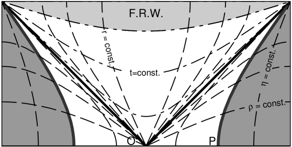
FIG. 1.: Conformal diagram showing a bubble expanding in a de Sitter background. The bubble wall is represented as the thick grey line starting at the point P. It expands with constant acceleration along a $\eta=const.$ surface. The FRW open universe is inside the future light cone from the point O, which is the center of symmetry of the bubble solution.

The purpose of this paper is to show that in models of this sort, with variable $\Omega$, the picture is actually more complicated. Indeed, instead of an infinite open universe inside of each bubble, what we find is an infinite number of inflating islands of finite size inside each bubble.

Quasi-open universes are not entirely new. The simplest two-field model of open inflation, where the tunneling field $\sigma$ and the slow-roll field $\phi$ are decoupled, is actually a quasi-open one, as emphasized by the authors of Ref. [5]. Quasi-openness is in principle not a desirable feature, since to a typical observer, the universe looks anisotropic [19]. In the simple “decoupled” model, this “classical” anisotropy is large and, combined with the effect of quantum “supercurvature” fluctuations mentioned above [8], it basically rules out the model [19].

To circumvent this problem, Linde and Mezhlumian introduced a class of two-field models where the slow-roll field is coupled to the tunneling field. As we shall see, these models are also quasi-open. This does not mean that they are not good cosmological models. If the co-moving size of the inflating islands is sufficiently large, then the resulting classical anisotropy may be unobservable. Even so, the fact that these islands are finite leads to a dramatically different picture of the large scale structure of the universe in open models.

The plan of the paper is the following. In Section II we briefly review the “supernatural” model of inflation, introduced in Ref. [5]. In this model, an approximate $U(1)$ symmetry is broken by a tunneling field in a first order phase transition, and slow-roll inflation inside the nucleated bubbles is driven by the pseudo-Goldstone boson. In section III, we study the quantum fluctuations of the pseudo-Goldstone in the bubble background. Section IV is the core of the paper, where we argue that after tunneling, we do not obtain an infinite open universe, but an infinite ensemble of quasi-open universes inside a single bubble. Section V is devoted to more general models, like the “coupled” and “uncoupled” two-field models. In Section VI we briefly describe the observational implications of our results and in Section VII we summarize our conclusions.

II Supernatural inflation

An attractive scenario for open inflation is the model of a complex scalar field with a slightly tilted mexican hat potential, see Fig. 2, where the radial component of the field does the tunneling and the pseudo-Goldstone does the slow-roll. This model was called “supernatural” inflation in Ref. [5], because the hierarchy between tunneling and slow-roll mass scales is protected by the approximate global $U(1)$ symmetry.

The action is given by

$${\cal S}=-\int\,d^{4}x\sqrt{-g}\,\Big{[}\partial_{\mu}\Phi^{*}\partial^{\mu}\Phi+V(\Phi,\Phi^{*})\Big{]},$$ (1)

where we use the metric signature $(-,+,+,+)$. Expanding the field in the form $\Phi=(\sigma/\sqrt{2})\exp(i\phi/v)$, where $v$ is the expectation value of $\sigma$ in the broken phase, we consider a potential of the form

$$V=V_{0}(\sigma)+V_{1}(\sigma,\phi)$$

where $V_{0}$ is $U(1)$ invariant and $V_{1}$ is a small perturbation that breaks this invariance. It is asumed that $V$ has a local minimum at $\Phi=0$ which makes the symmetric phase metastable. We shall consider a ‘tilt’ in the potential of the form $V_{1}=\Lambda^{4}(\sigma)G(\phi)$ where $\Lambda$ is a slowly varying function of $\sigma$ which vanishes at $\sigma=0$. For definiteness we can take $G=(1-\cos\phi/v)$.

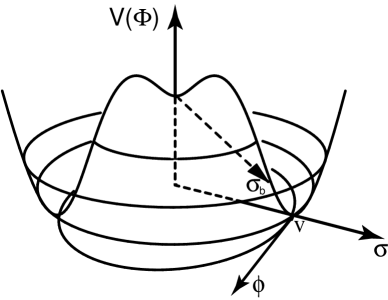
FIG. 2.: The inflaton potential for the supernatural model. An approximate U(1) symmetry is broken through bubble nucleation. We call $\sigma$ the tunneling direction and $\phi$ the direction orthogonal to it. The instanton $\sigma_{0}(\tau)$ interpolates between false vacuum at $\tau\to\infty$, and $\sigma_{b}$ at $\tau=0$.

The idea is that $\sigma$ tunnels from the symmetric phase $\sigma=0$ to the broken phase, landing at a certain value of $\phi$ away from the minimum of the tilted bottom. Once in the broken phase, the potential $V_{1}$ cannot be neglected, and the field $\phi$ slowly rolls down to its minimum, driving a second period of inflation inside the bubble. Another attractive feature of this model is that depending on the value of $\phi$ on which we land after tunneling, the number of $e$-foldings of inflation will be different. Hence it appears that in principle we can get a different value of the density parameter in each nucleated bubble. As we shall see, however, this picture is somewhat oversimplified.

We should point out that the supernatural model is not free from certain restrictions. Indeed, in order for the pseudo-Goldstone to realize inflation as in the simple free field “chaotic” scenario, we would need $v\gtrsim M_{p}$, where $M_{p}$ is the Planck mass. On the other hand, if $V_{0}$ is a typical quartic potential, the bubble walls would undergo topological inflation [20] for $v\gtrsim M_{p}$, and this would spoil the open scenario. Topological inflation occurs when the thickness of the walls is larger than the Hubble rate at the top of the potential barrier separating two local minima (degenerate or not). This is the same condition under which the Coleman-de Luccia instantons [2] cease to exist, and we have a Hawking-Moss [16] transition instead. Hence the condition $v\gtrsim M_{p}$ also represents the regime where the transition is not of the Coleman-de Luccia type, as it would be necessary for a successful open universe. As emphasized in Ref. [5] in the case of single-field open inflation, a transition of the Hawking-Moss type would leave unacceptable anisotropies in the CMB. These constraints can be made less severe by choosing a suitable form for $V_{0}$, with higher curvature at the top of the potential between the two minima, or perhaps a special form for $G$. In any case, we shall take $v\sim M_{p}$ in what follows.

III Quantum fluctuations

In this section, we compute the amplitude of quantum fluctuations of the pseudo-Goldstone field in the supernatural inflation model. For this, we need to review the formalism for quantizing fields in the background of a bubble.

The field equation for $\Phi$ is

$$\Box\Phi-{\partial V(\Phi)\over\partial\Phi^{*}}=0,$$ (2)

where $V=V_{0}+V_{1}$. In terms of the modulus $\sigma$ and phase $\phi/v$, we have

$$\Box(\sigma e^{i\phi/v})-\left[{\partial V(\sigma,\phi)\over\partial\sigma}+i{v\over\sigma}{\partial V(\sigma,\phi)\over\partial\phi}\right]e^{i\phi/v}=0.$$ (3)

It should be noted that classical solutions with $\phi=\tilde{\phi}=const.$ exist only if $\tilde{\phi}$ is an extremum of $G$, so that

$$\left.\partial V\over\partial\phi\right|_{\phi=\tilde{\phi}}=0.$$

This is true also for the Euclidean solutions (instantons) describing the tunneling, so strictly speaking these instantons can only take us from the false vacuum to the extrema of $V_{1}$ in the broken phase. Even if we relax the condition that $\phi$ should be constant, there may not be any instantons which can take us to non extremum values. Of course, this nonexistence of the corresponding instanton does not mean that the field cannot tunnel to a non-extremum value of $\phi$, it simply means that tunneling away from the extremum will be somewhat suppressed. This question will be addressed in Section IV.

Since the effect we are studying is not due to gravity, we shall start with the case of a bubble in flat spacetime. Including gravity is quite straightforward and will be done below. According to the theory of vacuum decay [1], the tunneling rate is dominated by the $O(4)$ symmetric solution of the Euclideanized equations of motion (3) with appropriate boundary conditions, which is called the instanton or bounce, and which we shall write as

$$\sigma=\sigma_{0}(\tau),\quad\phi=\tilde{\phi}=const,$$ (4)

Here, we have introduced the Euclidean radial coordinate $\tau\equiv({\bf X}^{2}+T_{E}^{2})^{1/2}$, where $(T_{E},{\bf X})$ are cartesian coordinates in Euclidean space. As we move from spatial infinity to the origin, the bounce interpolates between false vacuum $\sigma_{0}(\tau\to\infty)=0$ and a certain value of the field in the basin of the true vacuum, see Fig. 2, $\sigma_{0}(0)\equiv\sigma_{b}$. In addition, the bounce has to satisfy the boundary condition $\dot{\sigma}_{0}(0)=0$. The solution describing the bubble after nucleation is given by the analytic continuation of the instanton to Minkowski time $T$ through the substitution $T_{E}=-iT$. Then, the bubble solution depends only on the Lorentz invariant ‘distance’ to the origin $({\bf X}^{2}-T^{2})^{1/2}$, where $(T,{\bf X})$ are the usual Minkowski coordinates.

It is useful to change to the new coordinates

$$\tau=({\bf X}^{2}-T^{2})^{1/2},\quad\rho\equiv\tanh^{-1}(T/|{\bf X}|),$$ (5)

in terms of which the line element reads

$$ds^{2}=d\tau^{2}+a_{E}^{2}(\tau)d\Omega_{dS^{3}};$$ (6)

Here $d\Omega_{dS^{3}}=-d\rho^{2}+\cosh^{2}\rho(d\theta^{2}+sin^{2}\theta d\varphi^{2})$ is the line element of a 2+1 dimensional de Sitter space of unit ‘radius’, and in flat space $a_{E}(\tau)=\tau$. Including gravity, $a_{E}$ has to satisfy the (Euclideanized) Friedmann equation, as described below. This 2+1 dimensional de Sitter space can be thought as the hyperboloid swept by the bubble wall during its time evolution (suitably rescaled). In spite of its name, the coordinate $\rho$ is timelike, whereas $\tau$ is a ‘radial’ spacelike coordinate.

The above coordinates cover only the exterior of the light-cone from the origin. In order to cover the interior, which is where the open universe sits, we use the coordinates

$$t=(T^{2}-{\bf X}^{2})^{1/2},\quad r\equiv\tanh^{-1}(|{\bf X}|/T).$$ (7)

In terms of these the metric reads

$$ds^{2}=-dt^{2}+a^{2}(t)d\Omega_{H^{3}},$$ (8)

where $d\Omega_{H^{3}}=dr^{2}+\sinh^{2}r(d\theta^{2}+sin^{2}\theta d\varphi^{2})$ is the metric on the unit 3-dimensional hyperboloid and (in flat space) the scale factor is given by $a(t)=t$.

Notice that (8) is the metric of an open FRW. When gravity is included, the scale factor $a(t)$ will no longer be proportional to the cosmological time $t$ but it will be given by the solution of the Friedmann equation

$$(1-\Omega)=(aH)^{-2}.$$

In the general case, the metrics (6) and (8) are related by the analytic continuation of coordinates and scale factor in the following way

$$t=-i\tau,\quad r=\rho+i{\pi\over 2},\quad a(t)=-ia_{E}(it).$$ (9)

These relations can be used to analytically continue solutions from the outside to the inside of the light-cone from the origin.

In what follows, we shall assume that tunneling occurs along the real direction for $\Phi$, i.e. $\tilde{\phi}=0$ in (4), and we shall consider perturbations around the classical solution of the form

$$\sqrt{2}\Phi=\sigma_{0}(\tau)+\varphi_{1}+i\varphi_{2}.$$ (10)

Note that

$$\phi\simeq v\,{\varphi_{2}\over\sigma_{0}}\,.$$ (11)

Substituting into the action (1) we obtain the second order action for linearized perturbations

$$S^{(2)}=S_{0}[\sigma_{0}]+\int\,d^{4}x\sqrt{-g}[\Box\sigma_{0}-V_{0}^{\prime}(\sigma_{0})]\varphi_{1}+S_{1}[\varphi_{1}]+S_{2}[\varphi_{2}],$$ (12)

where

$$S_{1}=-{1\over 2}\int\,d^{4}x\sqrt{-g}\left(\partial_{\mu}\varphi_{1}\partial^{\mu}\varphi_{1}+V_{0}^{\prime\prime}(\sigma_{0})\varphi_{1}^{2}\right),$$ (13)

$$S_{2}=-{1\over 2}\int\,d^{4}x\sqrt{-g}\left(\partial_{\mu}\varphi_{2}\partial^{\mu}\varphi_{2}+\left[{V_{0}^{\prime}(\sigma_{0})\over\sigma_{0}}+m^{2}(\sigma_{0})\right]\varphi_{2}^{2}\right).$$ (14)

Here

$$m^{2}(\sigma_{0})={v^{2}\over\sigma_{0}^{2}}\Lambda^{4}(\sigma_{0})\,G^{\prime\prime}(0)={\Lambda^{4}(\sigma_{0})\over\sigma_{0}^{2}}$$ (15)

is a small $\tau$-dependent ‘squared mass’ due to the potential $V_{1}$. In the last equality we have used $G$ of the form $G=(1-\cos\phi/v)$. When the field $\sigma$ is in the broken phase, then $m$ is the mass of the pseudo-Goldstone. Of course, using the unperturbed equations of motion the linear term in (12) drops out.

The action (13) has been studied in some detail in the past [21, 13] because it is the same as the one for a one-field model. In particular, it describes the fluctuations of the bubble wall itself. Here, we shall concentrate on $S_{2}[\varphi_{2}]$, which describes fluctuations in the direction transverse to tunneling.

In order to study quantum fluctuations, the field $\varphi_{2}$ is expanded as a sum over modes times the corresponding creation and anihilation operators

$$\varphi_{2}=\sum\varphi_{plm}a_{plm}+h.c.$$ (16)

The equation of motion satisfied by the modes is

$$\Box\varphi_{plm}-\left[{V_{0}^{\prime}(\sigma_{0})\over\sigma_{0}}+m^{2}(\sigma_{0})\right]\varphi_{plm}=0.$$

Following [21, 13], we take the ansatz

$$\varphi_{plm}=a_{E}^{-1}(\tau)F_{p}(\tau){\cal Y}_{plm}(x^{i}),$$ (17)

where $x^{i}=(\rho,\theta,\varphi)$ are coordinates on the 2+1 de Sitter space spanned by the motion of the bubble wall. Introducing the conformal coordinate $\eta$ defined through the relation $a_{E}(\tau)d\eta=d\tau$, the equation of motion separates into a Schrödinger equation

$$-{d^{2}F_{p}\over d\eta^{2}}+a_{E}^{2}\left[{V_{0}^{\prime}(\sigma_{0})\over\sigma_{0}}+m^{2}(\sigma_{0})-{{\cal R}\over 6}\right]F_{p}=p^{2}F_{p},$$ (18)

where the separation constant $p^{2}$ plays the role of an energy eigenvalue, and a Klein-Gordon equation for the modes of a scalar field of mass $p^{2}+1$ living in the 2+1 dimensional de Sitter space

$$^{(3)}\Box{\cal Y}_{plm}=(p^{2}+1){\cal Y}_{plm}.$$ (19)

Here ${}^{(3)}\Box$ is the covariant d’Alembertian in this lower dimensional space, and ${\cal R}$ is the four-dimensional Ricci scalar, which from the unperturbed Einstein’s equations can be written as ${\cal R}=8\pi G[4V(\sigma_{0})+(\sigma_{0}^{\prime}/a_{E})^{2}]$.

The modes $\varphi_{plm}$ should be Klein-Gordon normalized on a Cauchy surface such as $\rho=0$. This amounts to Klein-Gordon normalizing the lower dimensional modes ${\cal Y}_{plm}$ in the 2+1 dimensional sense, and then normalizing $F_{p}$ as in the Schrödinger problem [21],

$$\int_{-\infty}^{\infty}F_{p}F_{p^{\prime}}d\eta=\delta_{pp^{\prime}},$$ (20)

where the delta function will be discrete or continuous depending on whether we are considering discrete or continuous eigenstates of the Schrödinger equation. In flat space, $a_{E}=R_{0}e^{\eta}$, where $R_{0}$ is an arbitrary constant which can be conveniently taken to be of order the radius of the bubble at the time of nucleation. Therefore, the effective potential in the Schrödinger equation

$$V_{\rm eff}(\eta)\equiv a_{E}^{2}\left[{V_{0}^{\prime}(\sigma_{0})\over\sigma_{0}}+m^{2}(\sigma_{0})-{{\cal R}\over 6}\right]$$ (21)

tends to zero at $\eta\to-\infty$ (center of the bubble) and to infinity at $\eta\to+\infty$ (false vacuum), see Fig. 3. In curved space, it can be shown that [2] $a_{E}(\eta\to\pm\infty)\to 0$, so $V_{\rm eff}$ vanishes at both ends. Therefore, in both cases, the spectrum will be continuous for $p^{2}>0$, and there may be a discrete spectrum for $p^{2}<0$.

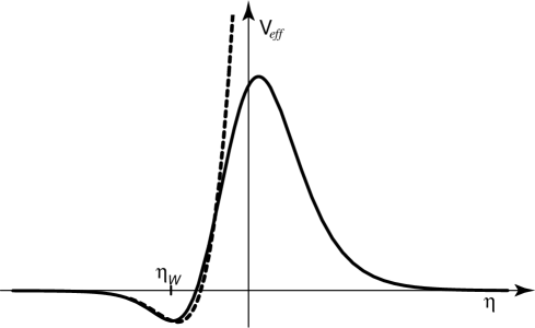
FIG. 3.: The effective potential in Eq. (21). In flat space (dashed line) the potential grows without bound at large $\eta$, whereas including gravity it tends to zero. At $\eta\to-\infty$, which corresponds to the center of the bubble, $V_{\rm eff}$ tends to zero.

A Quantum state of a nucleating bubble

In a time dependent background, the choice of a vacuum state is always somewhat ambiguous [22]. Here, this ambiguity corresponds to the freedom of choosing the ‘positive frequency’ modes ${\cal Y}_{plm}$ on the hyperboloid. In principle, the ambiguity can be resolved dynamically if the initial quantum state before the bubble nucleates is given.

The quantum state of a nucleating bubble has been extensively studied both in flat and in curved space [23]. In our model, $\varphi_{2}$ is treated as a free field which couples to the bubble via a $\sigma$-dependent mass term. For this type of models, it has been shown that if the initial quantum state is de Sitter invariant before the bubble nucleates, then right after bubble nucleation the field $\varphi_{2}$ will be in an $O(3,1)$ symmetric state. This is perhaps not too surprising: the appearance of the bubble breaks the $O(4,1)$ de Sitter symmetry by selecting a “nucleation point” in spacetime, but otherwise the bubble solution respects an $O(3,1)$ subgroup of isometries.

What this means is that the positive frequency modes ${\cal Y}_{plm}$ must be taken as the Bunch-Davies modes, which guarantee the desired symmetry. These are given by

$${\cal Y}_{plm}=\left[\frac{\Gamma(l+1-ip)\Gamma(l+1+ip)}{2}\right]^{1/2}\frac{P^{-l-1/2}_{ip-1/2}(i\sinh\rho)}{\sqrt{i\cosh\rho}}Y_{lm}(\theta,\phi).$$ (22)

where $P^{\mu}_{\nu}$ are the Legendre functions and $Y_{lm}$ are the usual spherical harmonics. When analytically continued to the inside of the light-cone, through the relations (9), they become

$${\cal Y}_{plm}=\left[\frac{\Gamma(l+1-ip)\Gamma(l+1+ip)}{2}\right]^{1/2}\frac{P^{-l-1/2}_{ip-1/2}(\cosh r)}{\sqrt{\sinh r}}Y_{lm}.$$ (23)

These are proportional to the often used harmonics $Y_{plm}$ which are normalized on the hyperboloid $H^{3}$ [9],

$${\cal Y}_{plm}={\Gamma(ip)\over\sqrt{2}}\sqrt{{\Gamma(l+1-ip)\over\Gamma(l+1+ip)}}Y_{plm}.$$

These analytically continued modes are normalizable on $H^{3}$ only for $p^{2}\geq 0$. Since the mode with $p^{2}=0$ has wavelength comparable to the curvature scale, the non-normalizable modes with $p^{2}<0$ have been dubbed “supercurvature” modes [9]. Writing $p=-i\Lambda$, the supercurvature modes are given by

$${\cal Y}_{\Lambda,lm}=\left[{\Gamma(\Lambda+l+1)\Gamma(-\Lambda+l+1)\over 2}\right]^{1/2}{P_{\Lambda-1/2}^{-l-{1/2}}(\cosh r)\over\sqrt{\sinh r}}\,.$$ (24)

(We have added a comma after the subindex $\Lambda$ to indicate that it is the value of $ip$ rather than $p$). We repeat, however that if the corresponding bound state exists in the Schrödinger equation (18), then these modes are perfectly normalizable on the Cauchy surface, and hence they must be included in the expansion of the field operator (16).

B Degenerate case

To begin with, let us neglect the mass term $m^{2}$ (15) which comes from the tilt in the potential, $V_{1}$ . Then, using the equation of motion satisfied by $\sigma_{0}$, it is straightforward to show that

$$F_{1}={\cal N}a_{E}\sigma_{0}$$ (25)

is a solution of (18) with eigenvalue $p^{2}=-1$, or $\Lambda=1$. Moreover, this solution is normalizable and it belongs to the discrete spectrum. The normalization constant ${\cal N}$ is found from (20)

$${\cal N}=\left(\int_{0}^{\tau_{max}}a_{E}\sigma_{0}^{2}(\tau)d\tau\right)^{-1/2}.$$ (26)

Here, we have changed back to the physical coordinate $\tau$, which measures the physical distance to the center of the bubble. In flat space $\tau_{max}$ is actually infinite, but the integral is finite because $\sigma_{0}$ vanishes exponentially fast outside the bubble. Including gravity $\tau_{max}$ becomes a finite value, so the integral is also finite. The explicit value of ${\cal N}$ can be calculated numerically for any given model. If $R_{0}$ is the size of the bubble and $\sigma_{b}$ is the value of the field at the center of the bubble, see Fig. 1, at the time of nucleation, then we can estimate

$${\cal N}\approx{\sqrt{2}\over R_{0}\sigma_{b}}.$$

The above estimate is for bubbles such that $R_{0}$ is small compared with the Hubble radius, so that $a_{E}\approx\tau$. Also, we have substituted $\sigma_{0}$ by $\sigma_{b}$ in the integrand, and we have integrated $\tau$ from zero up to $R_{0}$. Because $\sigma_{0}\leq\sigma_{b}$ our estimate is actually a lower bound on ${\cal N}$, and in some thick wall models the effect can be somewhat higher.

If we asume a large energy difference between false and true vacua, then we are in the thick wall regime and $R_{0}$ is of the order of the thickness of the bubble wall

$$R_{0}\sim M^{-1}.$$

Here $M$ is the mass of the field in the false vacuum. If, on the contrary, the vacua are sufficiently degenerate, then we are in the thin wall regime, and the expression for $R_{0}$ can be found e.g. in Appendix C and Ref. [25].

The normalized mode has an amplitude

$$\varphi_{1,lm}\approx{\sqrt{2}\over R_{0}}{\sigma_{0}(\tau)\over\sigma_{b}}{\cal Y}_{1,lm}(x_{i}).$$ (27)

Physically, what happens is that the field does not simply tunnel to a sharply defined value of $\phi$, but a distribution of values. Taking into account that the phase of our complex scalar field $\Phi$ is given by Eq. (11), the $x^{i}$ dependence in (27) shows that, after nucleation, different points on the bubble have different values of the angle $\phi$.

When analytically continued to the interior of the light-cone from the origin, through the relations $(\ref{analytical})$, $\tau$ is replaced with the cosmological time and $\sigma_{0}(t)$ quickly follows its evolution towards its expectation value $\sigma_{0}\approx v>\sigma_{b}$. Hence, inside the light-cone, the normalized supercurvature mode will take the form

$$\varphi_{1,lm}(t,r,\theta,\varphi)={\sqrt{2}\over R_{0}}{v\over\sigma_{b}}{\cal Y}_{1,lm}(r,\theta,\phi),$$ (28)

which is time independent. In order for the bubble solution to exist, the mass of the field in the false vacuum should be $M\gg H_{F}$, where $H_{F}$ is the Hubble rate in the false vacuum. In our model, $H_{F}$ is considered to be much greater than the Hubble rate in the true vacuum $H_{T}$. Therefore, the amplitude of supercurvature perturbations is of order $(v/\sigma_{b})M$. This exceeds by far the amplitude of the usual “subcurvature” fluctuations, which is only of order $H_{T}$. The corresponding effect in the CMB places severe constraints on the model [8]. We shall come back to this question in Section VI.

Note that for $\Lambda=1$ the amplitude of the homogeneous mode $l=0$ diverges because one of the gamma functions in (24) has vanishing argument. This is related to the fact that, strictly speaking, the $l=0$ mode should have been quantized as a collective coordinate instead of as a harmonic oscillator [26]. The divergence simply means that all values of $\phi$ are equally probable after nucleation. When we include the effect of $V_{1}$, the degeneracy will be broken and the $l=0$ mode will have a finite amplitude.

C Non-degenerate case

When the tilt $V_{1}$ in the potential is included, $p^{2}=-1$ is no longer an eigenvalue of the Schrodinger operator (18). However, it is clear that for small $m^{2}$ there will still be a discrete eigenmode whose eigenvalue we can calculate in perturbation theory. Denoting by $|-1\rangle$ the unperturbed bound state (25), the perturbation to the eigenvalue will be given by

$$\gamma\equiv p^{2}+1=\langle-1|a_{E}^{2}m^{2}|-1\rangle={\cal N}^{2}\int a_{E}^{4}\sigma_{0}^{2}m^{2}(\sigma_{0})d\eta.$$ (29)

Again, $\gamma$ can be computed numerically for any particular model, but we can estimate it as being of order

$$\gamma={\int a_{E}^{3}\sigma_{0}^{2}m^{2}(\sigma_{0})d\tau\over\int a_{E}\sigma_{0}^{2}(\tau)d\tau}\sim{1\over 2}R_{0}^{2}m_{b}^{2}\,,$$ (30)

where $m_{b}^{2}\equiv\Lambda^{4}(\sigma_{b})/\sigma_{b}^{2}$, see Eq. (15). The above estimate uses the same approximations as the estimate for ${\cal N}$ after Eq. (26).

The normalized $l=0$ mode will now be given by

$$\varphi^{\gamma}_{l=0}\approx{\cal N}\sigma_{0}{\cal Y}_{p,00}\approx{1\over\pi R_{0}}{\sigma_{0}(t)\over\sigma_{b}}{1\over\gamma^{1/2}}{\sinh[(1-\gamma)^{1/2}r]\over\sinh r}\ ,$$ (31)

where, from now on, we shall use the notation $\varphi^{\gamma}_{l}$ to denote the modes with $p^{2}=-1+\gamma$. In this expression, and the ones that will follow, we give only the unperturbed time dependence, without including the first order correction in $\gamma$. The field $\sigma_{0}(t)$ quickly rolls down from $\sigma_{b}$ and settles down to its minimum at $\sigma_{0}=v$. It is understood that, after that, the time derivative of the mode will be dominated by the corrections of order $\gamma$, which slowly drive the Goldstone modes to the minimum of the tilted potential. The amplitude of the higher-$l$ excitations will also suffer corrections of order $\gamma$, but since these amplitudes were already finite, the effect on those is not so dramatic. To leading order, the amplitudes are the ones calculated in the previous subsection.

It is interesting to look at the distribution of the field on a hyperboloid $t=const$. Note that the amplitude of the $l=0$ mode near the origin $r=0$ is of order

$$\varphi^{\gamma}_{l=0}(r\ll\gamma^{-1})\approx{1\over\sqrt{2}\pi}{\cal N}{\sigma_{0}\over\gamma^{1/2}}\approx{1\over\pi R_{0}\gamma^{1/2}}{\sigma_{0}\over\sigma_{b}},$$ (32)

which is a factor $\gamma^{-1/2}$ larger than the amplitude of the individual $l>1$ modes found in Eq. (28). But the amplitude of the $l=0$ mode decays exponentially for $r\gg\gamma^{-1}$, which means that at large distances it will become negligible. However, the quantum state that we have chosen is $O(3,1)$ symmetric, which means that the r.m.s. fluctuation of the field cannot depend on $r$. Therefore, the loss in amplitude of the $l=0$ mode as we move away from the origin has to be made up for by the joint contribution of the $l>0$ modes, smeared over a suitable length scale. This is analogous to what happens for a massive field in de Sitter space, except that here we are considering a spacelike manifold $t=const.$ rather than a spacetime. In the Appendix B we show that for $r\gg\gamma^{-1}$ we have

$$(\Delta\varphi^{\gamma})^{2}\equiv\sum_{l=1}^{l_{*}}(2l+1)(\varphi_{l}^{\gamma})^{2}\approx{{\cal N}^{2}\sigma_{0}^{2}\over 2\pi^{2}\gamma}\,l_{*}^{\gamma}\,e^{-\gamma r},$$

where $l_{*}\gg 1$ is a certain cut-off. If we smear over a fixed comoving length $\xi$, as we move away from the origin we have to include more and more modes in the sum. Since the $l$-th multipole has wavelength proportional to $(\sinh r)/l$, we take $l_{*}=\sinh r/\xi$. With this, we find $(\Delta\varphi^{\gamma})^{2}\approx({\cal N}^{2}\sigma_{0}^{2}/2\pi^{2}\gamma)(2\xi)^{-\gamma}$. Notice that the result is rather insensitive to the choice of $\xi$. As long as $|\ln\xi|\ll\gamma^{-1}$, the added contribution of all relevant modes at large $r$ is the same as the contribution of the $l=0$ mode near the origin, given by (32). We also show in Appendix A that the two-point correlations on a $t=const$ surface die off with comoving distance $d$ as $e^{-\gamma d/2}$.

Hence, around the time $t_{*}$ when the field $\sigma_{0}$ settles down to its minimum $\sigma_{0}\sim v$ the supercurvature fluctuations of the field are of order

$$(\Delta\varphi^{\gamma})\approx{\sqrt{2}\over\pi}\left({v\over\sigma_{b}}\right){1\over m_{b}R_{0}^{2}}={\sqrt{2}\over\pi}{\Lambda^{2}(v)\over\Lambda^{2}(\sigma_{b})}{1\over mR_{0}^{2}}\sim{M^{2}\over m}.$$ (33)

Here, $m=\Lambda^{2}(v)/v$ is the mass of the pseudo-Goldstone in the true vacuum. In the last step we have asumed that $\Lambda(\sigma)$ is a slowly varying function of $\sigma$, and set $R_{0}\sim M^{-1}$. Note that the fluctuation in $\varphi_{2}$ can easily reach Planckian values. It suffices to take $M\sim 10^{16}$ GeV and $m\sim 10^{13}$ GeV. With these values, the field is displaced enough from its minimum that it can drive inflation (recall that we are asuming $v\approx M_{p}$).

IV Quasi-open universe

Tunneling to a large value of the field is usually understood in an “adiabatic” sense. The idea is that since the motion of the phase is dictaded by the explicit symmetry breaking potential $V_{1}$, it will be much slower than the motion of the radial component of the field dictated by the large U(1) symmetric part of the potential. Hence, one can estimate the rate for tunneling at any $\phi$ by solving the Euclidean equations of motion for $\sigma$ while $\phi$ is kept as a frozen parameter. This frozen parameter is then used as the initial value of the slow-roll field on the $t=t_{*}$ hypersurface. Here, as above, $t_{*}$ is the time at which $\sigma_{0}$ reaches its expectation value $v$.

However, it is clear that when the spread of the pseudo-Goldstone on the $t=t_{*}$ hyperboloid is comparable to its range, $(\Delta\varphi^{\gamma})\gtrsim\pi v$, the picture that each bubble nucleates with a different value of $\varphi_{2}$ is not adequate. Instead, all of the ‘vacuum’ manifold is pretty much sampled inside a single bubble. In this case, inflation does not take place coherently on the $t=const.$ hyperboloids. As mentioned in the previous Section, the comoving correlation length for quantum fluctuations (in units of the curvature scale) is $d\sim\gamma^{-1}$. Thus, patches of comoving size $d\sim\gamma^{-1}$ where $\varphi_{2}$ is large and positive would be right next to patches where $\varphi_{2}$ is large and negative. These patches would be separated by regions where $\varphi_{2}$ is small and the universe does not inflate. Patches with positive and negative values can also be separated by “walls” where $\varphi_{2}$ is close to $\pi v$. In the case $v\approx M_{p}$ these domain walls of the pseudo-Goldstone potential would be topologically inflating [20]. Hence, instead of a smooth inflating hyperboloid, we have a patchy mosaic of inflating regions, as depicted in Fig. 4. In principle, each patch can give rise to a successful cosmology, but this cosmology will not be an open universe in the traditional sense. At best it will be a ‘quasi-open’ one, i.e. one which locally resembles an open FRW.

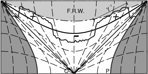
FIG. 4.: On a $t=const.$ hypersurface inside the bubble, the co-moving coherence length of the slow-roll field is $r\sim\gamma^{-1}$. If the r.m.s. fluctuations of the field are large, then regions where the field is large and positive will be next to regions where the field is large and negative. These will be separated by regions where the field is small and there is no second stage of inflation.

When $(\Delta\varphi^{\gamma})\ll\pi v$ the spread in the distribution of the pseudo-Goldstone in a $t=t_{*}$ section is small. What this means is that if the nucleated bubble is described by the $O(3,1)$ symmetric quantum state, then most of the surface $t=t_{*}$ has a non-inflating value of the field. However, in an infinite hypersurface, there will be a certain density of occasional large fluctuations which will lead to inflating islands of comoving size $d\sim\gamma^{-1}$. Each one of these islands will be a quasi-open universe.

This is in clear opposition with the conventional adiabatic picture described in the first paragraph. It is interesting to pursue the adiabatic picture for a moment, in order to see in which sense it is adequate or not. To keep the discussion simple, let us consider tunneling to a range of values of $\phi$ for which the linearized expressions (12) are still valid, but sufficiently large that it can be distinguished from tunneling to the bottom $\phi=0$. This will be the case if $\varphi_{2}$, see Eq. (11), is in the range

$$(\Delta\varphi_{2})\ll\varphi_{2}\ll v,$$ (34)

where $(\Delta\varphi_{2})^{2}=({\cal N}^{2}\sigma_{0}^{2}/2\pi^{2}\gamma)$ was computed in the previous section.

Since $\varphi_{1}$ and $\varphi_{2}$ decouple, we may take an approximate Euclidean solution of the form $\Phi=(1+i\phi/v)\sigma_{0}(\tau)/\sqrt{2}$, where $\phi$ is taken as constant in the adiabatic approximation. Substituting this configuration in the Euclideanized version of (12) we find, after straightforward algebra,

$$S_{E}[\phi]=S_{E}[\sigma_{0}]+{1\over 2}\int d^{4}x\sqrt{-g}\,m^{2}\varphi_{2}^{2}=S_{E}[\sigma_{0}]+{\gamma\pi^{2}\over{\cal N}^{2}v^{2}}\phi^{2}.$$

If the decay rate is proportional to $e^{-S_{E}}$, the relative probability of having a bubble with a certain value of $\varphi_{2}$ at nucleation will be

$${\cal P}(\varphi_{2})\sim\exp\left[{-\varphi_{2}^{2}\over 2(\Delta\varphi_{2})^{2}}\right],$$ (35)

where we have used (11) and, perhaps not too surprisingly, found $(\Delta\varphi_{2})^{2}=({\cal N}^{2}\sigma_{0}^{2}/2\pi^{2}\gamma)$, the same expression obtained in the previous section from considerations of quantum fluctuations in the $O(3,1)$ invariant state. Thus, two approaches which in principle are aimed at answering different questions end up giving the same answer. Here, we were asking how likely is it for a bubble to nucleate at a large value of $\phi$, whereas in the previous Section we were computing the amplitude of fluctuations inside a given bubble. Undoubtedly, both questions are related, since at least locally we cannot distinguish a large value of the field induced by the nucleation of the bubble from a fluctuation of the field inside the bubble.

However, even though the adiabatic approximation may give the right answer for the probability of tunneling to a large value of $\phi$, it suggests the wrong picture for bubble nucleation. Since $\phi=const$ is used in the above estimate, one might imagine that an infinite open universe with homogeneous $\varphi_{2}$ in the range (34) can be created. We shall argue that the probability for this to happen is actually zero. First of all, the formula $P\sim\exp[-S_{E}]$ is only justified when the Euclidean action is evaluated on a solution of the equations of motion. But $\phi=const$ is only a solution in the case when $V_{1}$ is neglected. We can try and correct this configuration so that it will be a solution, while still keeping $O(4)$ symmetry. In the linear regime, what this means is that we want a solution of Eq. (18) with $p^{2}=-1$, so that Eq. (19) is satisfied by ${\cal Y}_{plm}(x^{i})=const.$ and we have a homogeneous solution inside the bubble. However, for $m^{2}>0$ the lowest eigenvalue is $p^{2}=-1+\gamma>-1$, which means that the solution with $p^{2}=-1$ is not normalizable. As a result, the corresponding Euclidean action is badly divergent. If the action is regularized with a cut-off and if we take the $p^{2}=-1$ solution to be well behaved at the center of the bubble $\tau=0$, then it is easy to show that the action starts growing exponentially, $S_{E}\sim\exp[2M(\tau_{c}-R_{0})]$, as the cut-off $\tau_{c}$ in the radial direction $\tau$ becomes larger than the size of the bubble. Here $M$ is the mass of $\Phi$ outside the bubble. Hence it is not justified to say that the estimate (35) gives the nucleation rate for a homogeneous bubble. Rather, using a homogeneous solution we would get a divergent action and hence a vanishing probablility.

A Creation of a quasi-open universe

To compare, we can now ask what is the amplitude for tunneling from false vacuum to a spherically symmetric but inhomogeneous configuration with a large value of $\varphi_{2}$ inside the bubble. This is what we call an “inflating island” or quasi-open universe. Again, this amplitude will depend on the action of a semiclassical Euclidean trajectory. In order to make the metric (8) into one of Euclidean signature, we must consider the analytic continuation of the coordinates $t=-i\tau$ and $r=ir_{E}$. With this we have

$$ds^{2}=d\tau^{2}+a_{E}^{2}(\tau)d\Omega_{S^{3}},$$ (36)

where $d\Omega_{S^{3}}=dr_{E}^{2}+sin^{2}r_{E}(d\theta^{2}+sin^{2}\theta d\phi^{2})$ is the metric on the three-sphere, and the range of $r_{E}$ is from $0$ to $\pi$.

The semiclassical trajectory we shall consider is simply the analytic continuation of the $l=0$ supercurvature mode (31)

$$\varphi_{2}=A\ f(\tau)g(r_{E}),$$ (37)

where $f(\tau)=\sigma_{0}(\tau)+O(\gamma)$ and

$$g(r_{E})={\sin[(1-\gamma)^{1/2}r_{E}]\over\sin r_{E}.}$$

Note that this solution is not regular at one of the poles of the three-sphere, $r_{E}=\pi$. This is of course expected, since $g$ is an eigenfunction of the Laplacian with eigenvalue $\gamma$, which is not in the spectrum. Hence, (37) is not a regular “bounce” around which we should expand in order to find the false vacuum persistence amplitude [1]. This is not a problem for us here, because we are not estimating the total decay rate of the false vacuum but a particular transition amplitude. For this, we only need “half” of the Euclidean solution, which interpolates between false vacuum at $\tau\to\infty$, $r_{E}\approx 0$ and an inhomogeneous configuration at $r_{E}=\pi/2$. At $r_{E}=\pi/2$ this solution is matched to a Lorentzian solution at $\rho=0$ (the spacelike surface where the bubble nucleation takes place) simply by the analytic continuation $t=-i\tau$ and $\rho=i(r_{E}-\pi/2)$ [see Eq. (9)]. The solution is then propagated to the interior of the bubble (the “open” universe) through Eq. (9).

The transition amplitude $\Psi$ is WKB suppressed only in the Euclidean regime; the Lorentzian evolution contributing an oscillatory phase. Therefore

$$|\Psi|\sim e^{-S_{E}},$$

where

$$S_{E}=2\pi\int_{0}^{\infty}d\tau\ a_{E}^{3}(\tau)\int_{0}^{\pi/2}dr_{E}\ \sin^{2}r_{E}\left[\dot{\varphi}_{2}^{2}+{1\over a_{E}^{2}}\left({\partial\varphi_{2}\over\partial r_{E}}\right)^{2}+\left({V_{0}^{\prime}\over\sigma_{0}}+m^{2}\right)\varphi_{2}^{2}\right].$$

It is easy to show that since $\varphi_{2}$ is a solution of the equations of motion, after integration by parts the only contribution to the integral comes from the boundary term at $r_{E}=\pi/2$. A straightforward calculation gives

$$S_{E}=A^{2}\,{\gamma\pi^{2}\over 2}\int\ a_{E}^{2}\sigma_{0}^{2}d\eta\approx A^{2}\,{\gamma\pi^{2}\over 2{\cal N}^{2}},$$

where $A$ is de constant introduced in (37). After analytic continuation to the interior of the bubble, we have $\varphi_{2}(r\ll\gamma^{-1})\approx A\sigma_{0}$. Hence, the relative probability for nucleating through the inhomogeneous trajectory (37) is again given by

$${\cal P}=|\Psi|^{2}\sim\exp\left[{-\varphi_{2}^{2}\over 2(\Delta\varphi_{2})^{2}}\right].$$ (38)

Although this is in perfect agreement with (35), it is now clear that it doesn’t mean the whole open universe will have the value $\varphi_{2}$, but only a patch of comoving size $\sim\gamma^{-1}$ will have this value.

Thus, tunneling to a value of the field which is far from the one indicated by the $O(4)$ symmetric instanton is perfectly possible, with a somewhat suppressed probability. However, the resulting universe is not an infinite open universe but just a quasi-open one.

B Many universes in one bubble

The arguments used in the previos subsection leading to Eq. (38) are somewhat heuristic. In particular, we have not attempted to justify why the semiclassical trajectories of the form (37) should be the only relevant ones. Note, however, that the probability distribution (38) for nucleating at a high value of the field $\varphi_{2}$ near $r=0$, is the same as the Gaussian distribution for the amplitude of the $l=0,p^{2}=-1+\gamma$ mode in the $O(3,1)$ invariant state. In fact, the possibility of nucleating at different values of the field is already accounted for by this quantum state and need not be considered separately. The analysis of Refs. [23], whose result we described in Section III.A, takes into account all paths in $\phi$-field space, not just the semiclassical one used above. That analysis should be regarded as a more rigorous derivation of the result (38).

Because of the invariance of the quantum state, it is clear that there is nothing particular about the point $r=0$, and an inflating ‘blob’ is equally likely to develop around any point on the $t=t_{*}$ hyperboloid. Therefore we are led to the picture where in each comoving volume of size comparable to the correlation lenght $\gamma^{-1}$, the probability distribution for $\varphi_{2}$ is given by (38). Clearly, since the volume of the hyperboloid is infinite, inflating islands with all possible values of the field at their center will be realized inside of a single bubble. We may happen to live in one of those patches of comoving size $d\lesssim\gamma^{-1}$, where the universe appears to be open.

Also, in the supernatural model, it is possible to modify the shape of the potential near the false vacuum so that there is a misalignment between the prefered direction for tunneling [5] and the direction of the minimum of the pseudo-Goldstone potential in the broken phase. In this case, we expect that the $t=t_{*}$ surfaces inside the bubble will have a mean value of $\phi=\phi_{c}\neq 0$, determined by the most probable escape path (i.e., the instanton, which in this case will not land on $\phi=0$). This value of $\phi_{c}$ will determine the number of $e$-foldings of inflation and hence the mean value of the density parameter $\Omega_{0}$ on the hyperboloid. Let us call this value $\Omega_{c}$. If the tunneling path is not too narrow, there will still be a supercurvature mode which will cause fluctuations in the density parameter on co-moving scales of order $\gamma^{-1}$, which are of course much larger than the Hubble radius. The picture is then that we have an ensemble of large patches with different values of the density parameter. This is an interesting situation which deserves further study. However, since this model involves more parameters, for the remainder of this paper we shall concentrate on the simplest case discussed above, where the preferred tunneling direction and the minimum of the pseudo-Goldstone potential are aligned.

V More general models

In this section we shall consider the class of two-field models with a potential of the form

$$V(\sigma,\phi)=V_{0}(\sigma)+{1\over 2}m^{2}\phi^{2}+{1\over 2}g\sigma^{2}\phi^{2}.$$ (39)

Models of this type were introduced in Ref. [5]. Here $V_{0}$ is a non-degenerate double well potential, with a false vacuum at $\sigma=0$ and a true vacuum at $\sigma=v$. When $\sigma$ is in the false vacuum, $V_{0}$ dominates the energy density and we have an initial de Sitter phase with expansion rate given by $H_{F}^{2}\approx(8\pi G/3)V_{0}(0)$. Once a bubble of true vacuum $\sigma=v$ forms, the energy density of the slow-roll field $\phi$ may drive a second period of inflation.

As pointed out in Refs. [5], the simplest two-field model of open inflation, given by (39) with $g=0$ and $m\neq 0$, is actually a quasi-open one. Since there is no coupling between the two fields except for the gravitational one, we shall call this the “decoupled” two-field model. In this model, inflation starts chaotically at large values of $V(\sigma,\phi)\lesssim M_{p}^{4}$. In some regions of the universe, the field $\sigma$ will be trapped in the false vacuum, while $\phi$ rolls down from large values. If a bubble nucleates at a point where $\phi\sim M_{p}$, the value of the slow-roll field will be large enough to drive a short second period of inflation inside the bubble. One problem with this model, is that the slow-roll field moves also outside the bubble, so the synchronization of the $\phi=const.$ and $\sigma=const.$ surfaces inside the bubble is not perfect, as pointed out in Ref. [5].

In Ref. [19], the classical evolution of the slow-roll field from the outside to the inside of the bubble was studied, and it was found that on the hypersurface $t\sim H_{F}^{-1}$ the high value $\phi\sim M_{p}$ decays exponentially with the distance to the origin as

$$\phi\propto\exp[-\gamma_{c}r/2]$$ (40)

where $\gamma_{c}\approx{2m_{F}^{2}/3H_{F}^{2}}$. Hence, the size of the inflating region in this model is finite. We use the subindex $c$ to stress that this result follows from purely classical evolution. The larger $H_{F}$, the larger will be the inflating region. The reason is that the cosmological friction term in the equation of motion for $\phi$ is proportional to $H_{F}$, so the larger is $H_{F}$, the slower the field $\phi$ will roll down the potential outside the bubble, and the better is the synchronization between $\phi=const.$ and $\sigma=const.$ surfaces. However, $H_{F}$ cannot be taken to be too large because otherwise the quantum fluctuations generated outside the bubble produce too large an amplitude for the supercurvature mode inside the bubble [8]. The combination of these two effects severely constrains this model [19].

In order to construct a truly open model, Linde and Mezhlumian suggested taking $m=0$ and $g\neq 0$. We shall call this the “coupled” two-field model. In this way, the mass of the slow-roll field vanishes in the false vacuum, and it would appear that the problem of classical evolution outside the bubble is circumvented. However, this is not exactly so, and the whole class of models (39) leads to quasi-open universes. The basic reason is that, as we shall see below, the (linear) equation of motion for $\phi$ in the presence of the bubble, does not admit $O(3,1)$ invariant solutions which are regular at the origin, except for the trivial one, $\phi=0$. Thus, we are back to a situation analogous to the supernatural inflation model.

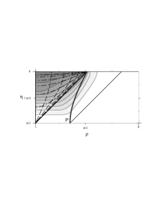
FIG. 5.: Conformal diagram of de Sitter space with a bubble expanding in it. Here $\eta$ and $\rho$ are the usual conformal coordinates in the closed chart. The bubble wall is represented by the curved thick line starting at the point P. The figure shows the result of a numerical evolution of the slow-roll field $\phi$ in the coupled model (39) with $m_{F}=0$ and $m_{T}=1.5H_{T}$. The self-gravity of the bubble has been ignored and we have taken $H_{T}=H_{F}$. The initial conditions for $\phi$ at $\eta=\pi/2$ are $\phi=const$ and $\dot{\phi}=0$. In spite of the fact that the field is massless outside the bubble, it starts evolving everywhere inside the light-cone from the point P. As a result, the surfaces of constant $\phi$, separating regions with different shadings, are not well synchronized with the $t=const.$ surfaces inside the bubble (see Fig. 1). In the plot, the field decays by one tenth of its initial value between consecutive $\phi=const.$ lines.

Even if the mass of the field in the false vacuum vanishes, one must not expect that $\phi$ will not evolve at all outside the bubble. Fig. 5 shows the result of a numerical evolution of the field $\phi$ in the coupled model. The figure represents a conformal diagram of a bubble expanding in de Sitter space (for simplicity, the gravitational field of the bubble has been neglected). The bubble wall is indicated by the thick timelike hyperbola. As initial conditions, we have taken $\phi=const.$ and $\dot{\phi}=0$. Surfaces of constant $\phi$ are indicated by different shadings. Even though the field is massless outside the bubble, we find that it does not stay exactly constant there. Due to the finite size of the bubble at the time of nucleation, the field $\phi$ feels the presence of the bubble everywhere inside the light-cone from the “point” P. As a result, inside the bubble, the hypersurfaces $\phi=const.$ are not perfectly synchronized with the $\sigma=const.$ hypersurfaces. Thus, we are back to a situation where the inflating region inside the bubble has a finite size, as in the decoupled model (note that the $\phi=const.$ lines cross the bubble wall trajectory).

Note that this effect is due to the finite size of the bubble. We shall see below that the effect is of order $(H_{F}R_{0})^{4}$. In Fig. 5, the parameters have been chosen so that the effect is very dramatic and the size of the inflating islands is comparable to the curvature scale, but one can choose parameters so that the inflating islands are as large as desired. However, except in the case where gravity is neglected so that $H_{F}=0$, their size is always finite and the large value of the field at the time of nucleation ends up decaying at large distances $r$ from the origin.

Hence, just as in the case of the supernatural model, the infinite $t=const.$ surfaces would be almost empty at large distances, if it wasn’t for the occasional quantum fluctuations which may ignite inflating islands here and there.

A Quantum fluctuations

As in the case of the supernatural model, we expand the field operator $\phi$ in terms of creation and anihilation operators,

$$\phi=\sum\varphi_{plm}a_{plm}+h.c.$$ (41)

In the present case, the equation of motion for the modes is given by

$$\Box\varphi_{plm}-[m^{2}+g\sigma_{0}^{2}]\varphi_{plm}=0.$$

Here $\sigma_{0}$ is the “background” bubble solution. Using the ansatz (17),

$$\varphi_{plm}=a_{E}^{-1}(\tau)F_{p}(\tau){\cal Y}_{plm}(x^{i}),$$

we have the following Schrödinger equation for $F_{p}$,

$$-{d^{2}F_{p}\over d\eta^{2}}+a_{E}^{2}\left[m^{2}+g\sigma_{0}^{2}-{{\cal R}\over 6}\right]F_{p}=p^{2}F_{p}.$$ (42)

This equation determines the spectrum of allowed eigenvalues $p^{2}$, which correspond to normalizable eigenfunctions $F_{p}$. All of these eigenvalues have to be included in the expansion of the field operator (41). As before, the harmonics ${\cal Y}_{plm}$ must satisfy equation (19).

In the case of supernatural inflation, we saw that there was a discrete eigenstate with $p^{2}<0$, which actually dominated the r.m.s. fluctuations of the field on a $t=const.$ hypersurface. We shall see that a similar situation happens in this case.

Since the Hubble rate inside the bubble $H_{T}$ is smaller than the Hubble rate outside, $H_{F}$, we need

$$m^{2}+gv^{2}\ll H_{T}^{2}<H_{F}^{2}$$ (43)

in order to have slow-roll inflation inside the bubble. This condition suggests taking a perturbative approach. To lowest order, we can neglect the mass term for $\phi$ and the gravitational backreaction of the bubble, so that $\phi$ is just a massless field in de Sitter space. In this case, Eq. (42) has the well known supercurvature mode with $p^{2}=-1$, which corresponds to [9]

$$F_{-1}={H_{F}\over\sqrt{2}}a_{E}(\eta)$$ (44)

The field configurations corresponding to this $p$ are $\phi=const.\times{\cal Y}_{1,lm}$. As mentioned before, for $l=0$ the harmonic ${\cal Y}_{1,00}$ is not Klein-Gordon normalizable in the 2+1 dimensional sense. This is because, for a massless field in de Sitter space, the zero mode corresponding to the translations $\phi\to\phi+const$ has to be treated as a collective coordinate and not as an oscillator. When the mass of $\phi$ is included, the mode becomes normalizable. Indeed, the bound state will shift to a perturbed eigenvalue $p^{2}=-1+\gamma$ which, as before, can be calculated perturbatively:

$$\gamma\equiv p^{2}+1={H_{F}^{2}\over 2}\int a_{E}^{4}\left[m^{2}+g\sigma_{0}^{2}-{{\cal R}\over 6}+2H_{F}^{2}\right]d\eta.$$ (45)

The normalized modes corresponding to the discrete eigenvalue take the form $\varphi^{\gamma}_{lm}\approx(H_{F}/\sqrt{2}){\cal Y}_{plm}(x^{i})$, and in particular, for the $l=0$ mode,

$$\varphi^{\gamma}_{l=0}\approx{H_{F}\over 2\pi}{1\over\gamma^{1/2}}{\sinh[(1-\gamma)^{1/2}r]\over\sinh r}[1+O(\gamma)].$$ (46)

The uncertainty of order $\gamma$ comes from the fact that we have not evaluated the correction to the “wave function” $F_{-1}$ which gives the temporal dependence of the field. This can be done in principle, but it is not really necessary for our purposes. It is clear that the mass term will cause the field to have the temporal dependence corresponding to slow-roll inside the bubble.

Near the origin $r=0$ the r.m.s. fluctuation of the field $\Delta\phi$ will be dominated by the mode (46), and for $t=t_{*}\sim H_{F}^{-1}$ it will be given by

$$\Delta\phi\approx{H_{F}\over 2\pi}{1\over\gamma^{1/2}}.$$ (47)

As mentioned in Section III, because of the $O(3,1)$ invariance of the quantum state, this will also be the r.m.s. fluctuation of the field at any point on the $t=t_{*}$ hypersurface (see Appendix B).

In the case of thin walls, the value of $\gamma$ can be calculated explicitly (see Appendix C),

$$\gamma={2\over 3}{m_{F}^{2}\over H_{F}^{2}}+{1\over 8}H_{F}^{2}R_{0}^{4}(m_{T}^{2}-m_{F}^{2}).$$ (48)

Here $m_{T}^{2}=m^{2}+gv^{2}$ is the mass of the slow-roll field in the true vacuum, $m_{F}^{2}=m^{2}$ is the mass in the false vacuum, $H_{F}$ is the hubble rate in the false vacuum, and $R_{0}$ is the intrinsic radius of the bubble at the time of nucleation.

The origin of the different terms in (48) is easy to understand. The first one is independent of the existence of the bubble, and comes from the fact that the slow-roll field has a mass $m_{F}^{2}$ in the false vacuum (the $H_{F}^{2}$ in the denominator can be understood from simple dimensional considerations). The second term is due to the perturbations of the effective potential in the Schrödinger equation (42) caused by the bubble solution. In the bubble, the scale factor $a_{E}$ is of order $R_{0}$, so the factor $a_{E}^{4}$ in the integrand of (45) will yield the factor $R_{0}^{4}$ in front of the second term of (48).

B Inflating islands

Even though the decoupled model ($g=0$) is not a very good candidate to an open cosmological model [19], it is instructive to consider it as a first step. In this model, inflation inside the bubble can be initiated because of the large “classical” value of $\phi$ at the time of nucleation, but at very large distances from the origin $r\gg\gamma^{-1}$, the classical field dies off, and only the quantum fluctuations remain.

Let us consider the amplitude of quantum fluctuations. From (48) we obtain ($m_{F}=m_{T}$)

$$\gamma={2m_{F}^{2}\over 3H_{F}^{2}}.$$

Accordingly, from (47), the r.m.s. quantum fluctuations of the field on the $t=t_{*}$ surfaces will be of order

$$(\Delta\phi)\approx\sqrt{3\over 2}{1\over 2\pi}{H_{F}^{2}\over m_{F}},$$ (49)

and the comoving correlation length will be of order $\gamma^{-1}=\gamma_{c}^{-1}$, the same as we found in the classical case (40) from a completely different approach.

In the decoupled model $m_{F}$ is the same as $m_{T}$, and $H_{F}$ is not too much larger than $H_{T}$ [5, 8, 19]. Since $H_{T}\sim m_{T}$, we have $(\Delta\phi)\ll M_{p}$ and quantum fluctuations on that surface would typically not reach “inflating” values of order $M_{p}$. Still, as in the supernatural model, an occasional large quantum fluctuation can initiate inflation on a patch of size $\gamma^{-1}$.

Let us reflect upon the meaning of Eq. (49). This r.m.s. amplitude is actually the same as the Bunch-Davies one for fluctuations of the slow-roll field outside the bubble [27]. Hence, the correct interpretation of the result (49) seems to be the following. Inflation inside and near the bubble wall may start because the field is large at the point where the bubble nucleates. However, even after bubble nucleation, the field will continue its random walk outside the bubble, and it may occasionally become large. If the bubble wall hits a patch where the field is large, then this will generate a local inflating patch inside the bubble, and we might inhabit one of those inflating patches. However, this model is not a very good open model, and it would only agree with observations if $\Omega_{0}$ were very close to one.

Let us now consider the “coupled” model, where the fields are coupled but $m_{F}=m=0$. In this case

$$\gamma\approx{1\over 8}m_{T}^{2}H_{F}^{2}R_{0}^{4}.$$

Clearly, by choosing parameters such that the size of the bubble is much smaller than the Hubble rate outside the bubble, or such that the mass of the field in the true vacuum is sufficiently small, $\gamma$ can be made as small as desired. Hence the size of inflating regions can be made as large as desired. In this case, the field is massless outside the bubble and quantum fluctuations of $\phi$ pile up to arbitrarily large values far from the bubble. However, from Eq. (47), we find a finite answer for the fluctuations inside the bubble

$$(\Delta\phi)\approx{\sqrt{2}\over\pi}{1\over m_{T}R_{0}^{2}}.$$ (50)

The first interesting thing to note about this result is that it does not depend explicitly on the Hubble rate inside or outside the bubble (the only dependence is through $R_{0}$). The second observation is that it is very similar to the expression (33) we had for the supernatural case, so a connection between the physics of both models can be anticipated. The finiteness of (50) is not surprising, since the slow-roll field is coupled to the bubble, and piling of modes in the vicinity of the bubble is suppressed by the mass term. Also, nucleation of bubbles at high values of $\phi$ is suppressed because the degeneracy between true and false vacuum is lower. As we discussed in Section IV, the quantum state already encodes the information that tunneling to a large value of the field is suppressed.

A difference with the supernatural inflation case is that now the amplitude of the supercurvature modes with $\l\neq 0$ is of order $H_{F}$ rather than $1/R_{0}$, hence the constraints on this model from microwave background anisotropies will be easier to accomodate.

VI Observational consequences

Our results from the previos sections have important consequences for two-field models of open inflation. First of all, our models are quasi-open, rather than open, which leads to classical anisotropies [19]. Second, we saw that in the supernatural model, the amplitude of supercurvature excitations is quite large. In this section, we shall give order of magnitude estimates for the expected CMB anisotropies from these effects. A detailed investigation of the power spectrum will be presented elsewhere [28].

A Classical anisotropies

Quasi-open universes are finite, and hence they look anisotropic to a typical observer. This effect was studied in Ref. [19] for the uncoupled model, and was called a “classical anisotropy”. The name was given because the finiteness of inflating islands was due to the classical motion of the slow-roll field outside of the bubble. Clearly, the same effect arises in all quasi-open universes we have considered. In some cases the appearance of the inflating island is better described as a semiclassical effect, but the resulting inflating islands are just as classical here as they were in Ref. [19]. Hence, we shall use the same name for this type of anisotropies.

To proceed, it will be important to distinguish between two different cases. The first case arises when the r.m.s. fluctuation of the slow-roll field $\phi$ on the spacelike surfaces $t=t_{*}\sim H_{F}^{-1}$ is small compared with $M_{p}$. In this case, “high peaks” where the field is comparable to $M_{p}$ and which will lead to inflating regions of co-moving size $r\sim\gamma^{-1}\gg 1$ will be very “rare” on that hypersurface. Here, $\gamma$ is the correction to the supercurvature eigenvalue, calculated in Section III.C for the supernatural model and in Section V.A for the more general models. High peaks of a homogeneous Gaussian random field tend to be spherical, and so our inflating islands will have approximate spherical symmetry. In the opposite case, when the r.m.s. fluctuation of the slow-roll field is comparable to $M_{p}$, we will have a patchy mosaic of “overlapping” inflating islands, as described in the second paragraph of Section IV. It is easy to check that in the second case the “classical” effect is small compared with the effect of quantum fluctuations which we shall consider in the next subsection, so here we shall only consider the first case.

Let us begin with the supernatural model. The quantum state we are considering leads to a Gaussian distribution for the random field $\phi$ that is $O(3,1)$ symmetric. Hence, to compute the probabilities for the field distribution around any point it suffices to study them around the origin $r=0$. Here we shall only be concerned with fluctuations due to the supercurvature modes, which have a long range. The effect of subcurvature modes can be incorporated in the usual way . Note that the r.m.s. amplitude for the $l=0$ supercurvature mode is a factor $\gamma^{-1/2}$ larger than the amplitude for $l>0$ modes (recall that $\gamma\ll 1$). Hence, even if the r.m.s. of $\phi$ is far below $M_{p}$, there is a certain probability for $\phi$ to reach $M_{p}$ in a certain region near the origin. The spherically symmetric mode is the one that is most likely to contribute to this possibility. Even though there is a small probability for this to happen, it is clear that only those rare regions with $\phi\sim M_{p}$ will undergo a second stage of inflation; so they will be the only ones that matter. The value of the field on those inflating islands will have the radial dependence of the $l=0$ mode, which decays as $\exp(-\gamma r/2)$ at large distances, $r\gg 1$.

Let us now discuss the more general models where the slow-roll field has a small mass or it is massless outside the bubble. In this case, one may ask what happens when a bubble nucleates in a place where the slow-roll field already had a large (classical) value. This may occur, for instance, if the whole universe was created at a large value of $\phi$, and at the time when the bubble nucleates $\phi$ is still rolling down from large values. This possibility would in principle be relevant for bubbles nucleated at early times, and is the one considered in [19]. However, as time goes by, the initially large classical value of the slow-roll field in the false vacuum will decrease, and all that will remain are the quantum fluctuations which should be well described by the $O(4,1)$ or de Sitter-invariant quantum state.

Occasionally, fluctuations of the slow-roll field in the false vacuum may create a localized region with a higher value of the field. The nucleation of a bubble on top of one of these regions will not be very different from the case discussed in the previous paragraph. Whether the bubble nucleates on one of these high peaks or not, the field outside the bubble will continue to fluctuate, and the bubble walls will from time to time bump into regions with a higher value of the field, as discussed in Section V.B. Hence, also in this case, there will be an ensemble of inflating regions with some distribution inside the bubble. From a formal point of view, notice that the appearance of the bubble has selected a point in spacetime, thus breaking the $O(4,1)$ invariance, but otherwise respects a residual $O(3,1)$ symmetry. Therefore it seems reasonable to expect that, at least in a statistical sense, the field inside the bubble will be well described by the $O(3,1)$ invariant Gaussian distribution, corresponding to the quantum state we have studied. Just as in the case of the supernatural model, here we also expect that the high peaks which lead to inflating islands will have spherical symmetry, and the value of the field on those islands will have the radial dependence of the $l=0$ mode, which decays as $\exp(-\gamma r/2)$ at large distances from the center of the island.

The co-moving size of the inflating islands is $r\sim\gamma^{-1}\gg 1$. Since the volume on the hyperboloid grows exponentially with the distance to the origin, as $\sinh^{2}rdr$, a typical observer in a quasi-open universe is most likely to be at $r\gg 1$, where the scalar field behaves as $\phi\propto\exp(-\gamma r/2)$. Up to exponentially small corrections, this is the same radial dependence that was considered in [19]. In that case, the fields were uncoupled and $\gamma=2m_{F}^{2}/3H_{F}^{2}$. The arguments used in [19] to estimate the temperature anisotropies measured by a typical observer can be directly applied to the models discussed here. Changing from the coordinates $(r,\theta,\phi)$ to a new set $(r^{\prime},\phi^{\prime},\theta^{\prime})$ such that the point $r=r_{0},\theta=0$ (with $r_{0}\gg 1$) is the new origin of coordinates, one finds that the perturbation of the field $\phi$ around $r^{\prime}=0$ can be described as [19] $\delta\phi=\phi_{0}(t)(\gamma/2)\ln f$, where $f\equiv(\cosh r^{\prime}+\sinh r^{\prime}cos\theta^{\prime})$ and $\phi_{0}$ is the value of the field at the point $r^{\prime}=0$. The corresponding gauge invariant potential at horizon crossing is

$$\Phi\approx{3\over 5}\left.{H_{T}\delta\phi\over\dot{\phi}_{0}}\right|_{t\approx H_{T}^{-1}}={3\over 5}{H_{T}^{2}\over m_{T}^{2}}{\gamma\over 2}\ln f(r^{\prime},\theta^{\prime}).$$ (51)

The effect on the microwave background temperature fluctuations can be computed by integrating the Sachs-Wolfe effect along the line of sight [29]. The dominant effect is in the quadrupole [19], and it is of order

$$\left.{\delta T\over T}\right|_{l=2}\sim 10^{-1}{H_{T}^{2}\over m_{T}^{2}}{\gamma\over 2}(1-\Omega_{0}).$$ (52)

This is just a very rough order of magnitude estimate, which works well for $\Omega_{0}\gtrsim 0.3$. A more detailed study of the power spectrum of temperature anisotropies will be presented elsewhere [28].

Note that if the universe is sufficiently flat, the factor $(1-\Omega_{0})$ may completely erase the effect. Otherwise, for a universe with appreciable curvature, we obtain a constraint on $\gamma$,

$$\gamma\lesssim{2\over(1-\Omega_{0})}{m_{T}^{2}\over H_{T}^{2}}\,10^{-4}.$$ (53)

where we have used $\delta T/T\lesssim 10^{-5}$, from the requirement that this effect does not dominate the temperature anisotropies on large scales, as seen by COBE [30]. Since $H_{T}$ is larger than $m_{T}$, it is clear that $\gamma$ has to be very small in order to avoid large temperature fluctuations.

In the supernatural model, $\gamma\sim R_{0}^{2}m^{2}/2$, this constraint implies

$$R_{0}\lesssim 2\times 10^{-2}(1-\Omega_{0})^{-1/2}H_{T}^{-1}$$

which is not difficult to accomodate. Note that the size of the bubble $R_{0}$ is necessarily less than the Hubble radius in the false vacuum and hence can easily be much less than the Hubble radius in the true vacuum. However, in the decoupled model discussed in [19] the constraint (53) forces $H_{T}$ to be quite large, and this causes a problem of large quantum fluctuations in the supercurvature modes [8].

In the class of models (39), the size of $\gamma$ is determined by Eq. (48). Clearly, the effect can be made small by choosing parameters such that $m_{F}$ and the size of the bubble are sufficiently small. This is not always straightforward to implement. For instance, the “hybrid” open inflation model considered in Ref. [7] turns out to be quasi-open and suffers from too large semiclassical anisotropies. However, it is possible to write an open hybrid model, with a massless inflaton in the false vacuum, that satisfies the constraints [28].

B Supercurvature anisotropies

In the previous subsection we have considered the case where the $l=0$ mode was “oversized”, meaning that it took an amplitude much larger than its expected r.m.s. Because of this, an observer far from the center of the inflating region would see the anisotropy (51). In this section we shall estimate the anisotropies caused by the $l>0$ supercurvature modes. Here we are not thinking that these higher modes are “oversized”; they simply take random values of the order of their r.m.s. For simplicity, we shall consider an observer located at $r=0$, but the effect should not be much different for an observer located elsewhere.

The size of CMB anisotropies caused by the $l>0$ supercurvature modes has been estimated in [9, 8]. For the class of models (39), where the supercurvature mode is normalized as in (44), the quadrupole CMB anisotropies are of order

$$\left.{\delta T\over T}\right|^{sup}_{l=2}\sim(1-\Omega_{0}){H_{F}\over H_{T}}\left.{\delta T\over T}\right|^{sub}_{l=2}\,.$$ (54)

Here $(\delta T/T)^{sub}$ are the temperature anisotropies caused by the subcurvature modes (with $p^{2}>0$). The supercurvatre effect decreases very fast with multipole number, basically as $(1-\Omega_{0})^{l/2}$. If the fluctuations we observe in the CMB are due to inflation, then we need $(\delta T/T)^{sub}\sim 10^{-5}$, and from (54) we have that $H_{F}$ cannot be too much larger than $H_{T}$, unless the universe is almost flat.

For the supernatural model, the supercurvature mode (28) has a normalization $2/(H_{F}R_{0})$ times larger than its counterpart (44) [we are ignoring the mild enhancement due to the factor $(v/\sigma_{b})$]. Hence, the analog of (54) is

$$\left.{\delta T\over T}\right|^{sup}_{l=2}\sim(1-\Omega_{0}){2\over H_{T}R_{0}}\left.{\delta T\over T}\right|^{sub}_{l=2}\,.$$ (55)

Therefore we need $R_{0}\gtrsim H_{T}^{-1}$. Since $R_{0}$ has to be necessarily smaller than $H_{F}^{-1}$, we have a two-fold restriction. On one hand, $R_{0}\sim H_{F}$, and on the other $H_{T}\sim H_{F}$. Thus, it seems fair to say that the model is not as natural as it was thought to be [5]: the difference in energy density between the true and the false vacuum cannot span many orders of magnitude. The reason is the following: In spite of the fact that the field is massive in the false vacuum, a supercurvature mode exists. Its normalization is not proportional to $H_{F}$ as in the usual case (39), but to $R_{0}^{-1}$, which is even larger. The effect can be thought as the excitation of the pseudo-Goldstone modes due to the acceleration of the domain wall “boundary”. The model may still be viable in a certain range of parameters. Determining this range requires detailed analysis, which is left for future research [28].

VII Conclusions

Open inflation is an appealing way of reconciling an infinite open universe with the inflationary paradigm. In this scenario, a symmetric bubble nucleates in de Sitter space, and its interior undergoes a second stage of slow-roll inflation to almost flatness. Single-field models of open inflation can in principle be constructed, but it does not seem possible to do so without a certain amount of fine tuning [5]. The basic problem is that there is a hierarchy between the large mass needed for successful tunneling and the small mass required for successful slow-roll. For that reason, it seems natural to consider two-field models of open inflation [5] where one field does the tunneling and the other drives slow-roll inflation inside the bubble.

In this paper we show that a large class of two-field models of open inflation do not lead to infinite open universes, as it was previous thought, but to an ensemble of inflating islands of finite size. The reason is that the quantum tunneling does not occur simultaneously along both field directions, and the equal-time hypersurfaces in the open universe are not synchronized with equal-density or fixed-field hypersurfaces. Technically, one finds that there are no $O(4)$ invariant instantons for the two-field system which would describe the formation of a bubble with “large” values of the slow-roll field in its interior. Large values of the inflaton field, needed for the second period of inflation inside the bubble, only arise as localized fluctuations. The interior of each nucleated bubble will contain an infinite number of such inflating regions, giving rise to a rather unexpected form of the large scale structure of the universe in these models.

The picture is the following. Right after the bubble has nucleated there will be, on the $t=const.$ hypersurfaces inside the bubble, a certain density of occasional large fluctuations of the slow-roll field that lead to inflating islands. This fluctuations are caused by modes whose wavelength is larger than the curvature scale. Denoting by $\gamma$ the eigenvalue of the Laplacian on the unit Hyperboloid (with $\gamma<1$), the co-moving size of the inflating islands is given by $d\sim\gamma^{-1}$ [The parameter $\gamma$ can be determined in terms of the parameters of the model, see Eqs. (30) and (48), and it is important in deriving observational constraints]. Each one of the inflating islands will be a quasi-open universe. Since the volume of the hyperboloid is infinite, inflating islands with all possible values of the field at their center will be realized inside of a single bubble. We may happen to live in one of those patches where the universe appears to be open. The fact that the inflating regions are finite gives rise to classical anisotropies like those discussed in Ref. [19].

In particular, we have studied the supernatural model introduced by Linde and Mezhlumian [5]. We have shown that in spite of the large mass of the inflaton field in the false vaccuum, there is a supercurvature mode. Its amplitude is proportional to $R_{0}^{-1}$, rather than the usual $H_{F}$. Here $R_{0}$ is the radius of the bubble at the time of nucleation and $H_{F}$ is the Hubble rate in the false vacuum. Since $R_{0}^{-1}>H_{F}$, this effect is quite important. In order to make the model compatible with observations, it is required that the energy density in the false vacuum should not be much larger than in the true vacuum. This means that $H_{F}/H_{T}$ cannot span many orders of magnitude, as it was previously believed [5]. The supercurvature mode can be understood as the pseudo-Goldstone mode associated with the choice of a tunneling direction in field space. Combining the supercurvature anisotropies with the classical ones we find that the range of $\Omega_{0}$ will also be restricted. Detailed analysis is required in order to determine the range of parameters in which the model may still be viable [28].

For the more general class of models (39), the size of the inflating islands can be chosen to be comfortably large by an appropriate choice of parameters. In this way, the classical anisotropy will be unobservably small. By order of magnitude, the constraint is given by Eq. (53), where $\gamma$ is given in Eq. (48). The constraint will be satisfied if the mass of the slow-roll field is sufficiently small in the false vacuum and $R_{0}$ is much smaller than $H_{F}^{-1}$. In a future publication [28] we will give more precise constraints from the observed power spectrum of temperature anisotropies of the CMB.

Finally, there are some two-field models of open inflation, such as the one introduced by Green and Liddle [6] in the context of induced gravity, which need not be affected in principle by the classical anisotropies mentioned above. In these models, the value of $\Omega_{0}$ is not variable; it is determined in terms of the parameters in the potential. It would be interesting to check whether $O(4)$ symmetric instantons do indeed exist in this model.

A

We will show in this Appendix that the two-point function on a $t=const$ surface for the state $\varphi^{\gamma}$ dies off as $e^{-\gamma d/2}$, where $d$ is the comoving distance between the points. We will compute the two-point function ouside the lightcone, and then continue it to the inside.

To compute the two-point function for $\varphi_{2}$, hereafter $G_{\varphi_{2}}(x,x^{\prime})$, we will use the fact that the modes ${\cal Y}_{plm}$ are properly normalized as Klein-Gordon modes of mass $p^{2}+1$ living in the $\tau=const.$ (2+1) de Sitter hypersurfaces of the outside lightcone metric. Thus we can define the fields

$${\cal Y}_{p}=\sum_{lm}{\cal Y}_{plm}\,{}^{dS}a_{lm}^{(p)}+h.c,$$ (A1)

and the de Sitter invariant vaccuum $|0\rangle_{dS}^{(p)}$ anihilated by ${}^{dS}a_{lm}^{(p)}$. Notice that $d\Omega_{dS}$ in (6) corresponds to the line element of a closed coordenization of a (2+1) de Sitter space, for which the two-point functions can be found in Ref. [31].

We can now write the two-point function $G_{\varphi_{2}}$ in terms of the two-point functions for ${\cal Y}_{p}$,

$$G_{\varphi_{2}}(x,x^{\prime}) = \langle 0|\varphi_{2}(x)\varphi_{2}(x^{\prime})|0\rangle=a_{E}^{-2}\sum_{plm}F_{p}(\tau)\overline{F_{p}(\tau^{\prime})}{\cal Y}_{plm}(x^{i})\overline{{\cal Y}_{plm}(x^{\prime i})}$$ (A2)

$$= a_{E}^{-2}\sum_{p}F_{p}(\tau)\overline{F_{p}(\tau^{\prime})}{}_{dS}\langle 0|{\cal Y}_{p}(x^{i}){\cal Y}_{p}(x^{\prime i})|0\rangle_{dS},$$ (A3)

where the sum over p has to be understood like a sum over the discrete eigenvalues $p^{2}$ of the Schrödinger equation (18) and like an integration over its continuum spectrum $p^{2}>0$. On a given $\tau=const$ hypersurface, the $\rho$ dependence of $G_{\varphi_{2}}(x,x^{\prime})$ will be given by $G_{p}(x^{i},x^{\prime i})$, weighted for each $p$ by $a_{E}^{-2}||F_{p}||^{2}$. The two-point function $G_{p}$ can be found in [31]

$$G_{p}(\xi,\xi^{\prime})=\frac{1}{(4\pi)^{3/2}}\frac{\Gamma(1-ip)\Gamma(1+ip)}{\Gamma(3/2)}F\left(1+ip,1-ip;\frac{3}{2};\frac{1+Z}{2}\right),$$ (A4)

where $F$ is the hypergeometric function and $Z$ is the scalar product of the position vectors at points $x^{i}$ and $x^{\prime i}$ in the embedding (3+1) Mikowski space,

$$Z(x^{i},x^{\prime i})=\xi^{\mu}(x^{i})\xi_{\mu}(x^{\prime i})=cos\tilde{\gamma}\cosh\rho\cosh\rho^{\prime}-\sinh\rho\sinh\rho^{\prime}.$$ (A5)

Here $\tilde{\gamma}$ is the angle on the 2-sphere between the two points. We recall that for the lowest discrete eigenmode to first order in the shift $\gamma$, $ip=1-\gamma/2$, so we will denote by $G^{\gamma}$ the two-point function for this eigenmode.

Now we have to analytically continue (A4) to the inside of the lightcone by means of (9). This amounts only to analytically continuing the scalar product $Z$,

$$Z(x^{i},x^{\prime i})\rightarrow-cos\tilde{\gamma}\sinh r\sinh r^{\prime}+\cosh r\cosh r^{\prime}.$$ (A6)

Taking $r^{\prime}=0$ and $r=d$, so $Z=\cosh d$, and using eq. (9.131.1) in Ref. [32], we find that inside the light-cone the two-point function between points separated a comoving distance $d$ can be written as

$$G^{\gamma}(d)=\frac{1}{(4\pi)^{3/2}}\frac{\Gamma(2-\gamma/2)\Gamma(\gamma/2)}{\Gamma(3/2)}\left(\frac{1-\cosh d}{2}\right)^{-\gamma/2}F\left(\frac{\gamma}{2},\frac{\gamma-1}{2};\frac{3}{2};\frac{1+\cosh d}{\cosh d-1}\right).$$ (A7)

As $d\rightarrow\infty$, the hypergeometric function in (A7) tends to a constant, and the assymptotic behaviour of $G^{\gamma}$ is given by

$$G^{\gamma}(d)\rightarrow\frac{1}{(4\pi)^{3/2}}\frac{\Gamma(\gamma/2)\Gamma(2-\gamma)}{\Gamma(3/2-\gamma/2)}\left(\frac{-1}{4}\right)^{-\gamma/2}\,e^{-\gamma d/2},$$ (A8)

which dies off exponentially with $d$.

Here, we have only computed the first term in the sum (A3). The terms with $p^{2}>0$ decay as $e^{-r/2}$, and hence they are subdominant at large distance.

B

To compute $(\Delta\varphi_{2}^{\gamma})^{2}$ for large $r$, we will need the asymptotic expressions for the hyperbolic harmonics ${\cal Y}_{\Lambda,lm}$ for $r\gg\gamma^{-1}$. The Legendre functions are given by (see e.g. Ref. [33])

$$P^{-1/2}_{\nu-1/2}(\cosh r)=\sqrt{2\over\pi}{\sinh\nu r\over\nu\sqrt{\sinh r}},$$ (B1)

From equation (23), the supercurvature mode ${\cal Y}_{\Lambda,00}$ is given by

$${\cal Y}_{\Lambda,00}={1\over\pi}\left[\frac{\Gamma(1-\Lambda)\Gamma(1+\Lambda)}{4}\right]^{1/2}\frac{\sinh\Lambda r}{\Lambda\sinh r},$$ (B2)

where $\Lambda=1-\gamma/2$. For large $r$, we have

$${\cal Y}_{(1-\gamma/2),00}\to{e^{-r\gamma/2}\over\pi\sqrt{2\gamma}}[1+O(\gamma)].$$ (B3)

For $l>0$, we can express $P^{-l-1/2}_{\nu}$ in terms of $P^{-1/2}_{\nu+k}$ using the recursion formula

$$P^{\mu}_{\nu}(z)=\frac{1}{2\nu+1}\frac{1}{\sinh r}\left(P^{\mu-1}_{\nu+1}(z)-P^{\mu-1}_{\nu-1}(z)\right).$$ (B4)

The Legendre function $P_{\nu}^{-l-1/2}$ acquires then the form

$$P^{-l-1/2}_{\nu}=\frac{1}{\sinh^{l}r}\sum_{k=-l}^{l}C_{k}(\nu)P^{-1/2}_{\nu+k},$$ (B5)

where $C_{k}(\nu)$ are some functions depending on $\nu$. In fact, for large $r$, we do not need to compute all $C_{k}(\nu)$. We have to take into account that for a supercurvature mode, $P^{-1/2}_{\nu}(\cosh r)$ behaves for large $r$ as $e^{|\nu|r}$ (as can be seen from (B1)). Thus, for the supercurvature mode $\nu=(1-\gamma)/2$, the term $k=l$ in (B5) grows exponentially faster than the rest of terms in the sum, so the main contribution for large $r$ will be given by this term. The coefficienty $C_{l}(\nu)$ can be easily read from (B4):

$$C_{l}(\nu)=\frac{\Gamma(\nu+1/2)}{2^{l}\Gamma(\nu+1/2+l)}.$$ (B6)

For large $r$, using (B5), (B6) and (23), we obtain

$${\cal Y}_{(1-\gamma/2),lm}\to\left[\frac{\Gamma(l+\gamma/2)}{\pi(1-\gamma/2+l)(l-\gamma/2)\Gamma(l-\gamma/2)}\right]^{1/2}\Gamma(1-\gamma/2)e^{-\gamma r/2}Y_{lm}(\Omega).$$ (B7)

Finally, using $\lim_{x\to\infty}\Gamma(x+a)/\Gamma(x)=x^{a}$, we can write ${\cal Y}_{(1-\gamma/2),lm}$ for large $l$, to order $\gamma$, as

$${\cal Y}_{(1-\gamma/2),lm}\approx\frac{l^{\gamma/2-1}}{\sqrt{\pi}}e^{-r\gamma/2}Y_{lm}(\Omega)[1+O(\gamma)].$$ (B8)

Using the results derived above, we can compute the amplitude of the $l=0$ mode near the origin,

$$\left.(\varphi_{l=0}^{\gamma})^{2}\right|_{r=0}=\left.({\cal N}\sigma_{0})^{2}{\cal Y}_{\Lambda,00}\overline{{\cal Y}_{\Lambda,00}}\right|_{r=0}\approx\frac{1}{\pi^{2}R_{0}^{2}\gamma}\left(\frac{\sigma_{0}}{\sigma_{b}}\right)^{2}[1+O(\gamma)],$$ (B9)

and for large $r$,

$$(\varphi_{l=0}^{\gamma})^{2}\to\frac{1}{\pi^{2}R_{0}^{2}\gamma}\left(\frac{\sigma_{0}}{\sigma_{b}}\right)^{2}e^{-r\gamma}=\left.(\varphi_{l=0}^{\gamma})^{2}\right|_{r=0}e^{-r\gamma}$$ (B10)

As we can see, the amplitude of the mode $l=0$ decays exponentially for $r\gg\gamma^{-1}$. Taking into account that we have choosen an $O(3,1)$ symmetric vaccuum, this decrease in amplitude for large $r$ must be compensated by the joint contribution of the $l>0$ modes, smeared over a suitable length scale, in such a way that the r.m.s fluctuations of the field are independent of $r$. Let us check it. We need to compute

$$(\Delta\varphi_{2}^{\gamma})^{2} \equiv \sum_{l=1}^{l_{*}}\sum_{m={-l}}^{l}\varphi^{\gamma}_{i\Lambda,lm}\overline{\varphi^{\gamma}_{i\Lambda,lm}}\to({\cal N}\sigma_{0})^{2}\sum_{l=1}^{l=l_{*}}\frac{(2l+1)}{4\pi}\frac{l^{\gamma-2}}{\pi}e^{-\gamma r}$$ (B11)

$$\approx ({\cal N}\sigma_{0})^{2}\frac{e^{-\gamma r}}{2\pi^{2}}\int^{l_{*}}_{0}l^{\gamma-1}\,dl\approx({\cal N}\sigma_{0})^{2}\frac{e^{-\gamma r}}{2\pi^{2}}\frac{l_{*}^{\gamma}}{\gamma},$$ (B12)

where $l_{*}$ is a certain cutoff, which has to grow as we move away from the origin to include more and more modes in the sum. If we smear the field over a fixed comoving lenght $\xi$, realizing that the wavelength of the $l$-th multipole is proportional to $(\sinh r)/l$, we can take $l_{*}=\sinh r/\xi$. Finally, we obtain

$$(\Delta\varphi_{2}^{\gamma})^{2}\to\frac{1}{\pi^{2}R_{0}^{2}\gamma}\left(\frac{\sigma_{0}}{\sigma_{b}}^{2}\right)(2\xi)^{-\gamma}\approx\left.(\varphi_{l=0}^{\gamma})^{2}\right|_{r=0}(1-\gamma\ln 2\xi).$$ (B13)

As we can see, as long as $|\ln 2\xi|\ll\gamma^{-1}$, the added contribution of the relevant modes is the same as the one given by the $l=0$ mode near the origin.

C

In the thin wall approximation, neglecting gravitational backreaction, the background geometry is found [25] to be described by two de Sitter pieces with different Hubble constant glued together at some $\eta_{W}$. The scale factor is given by

$$a_{E}(\eta)=a_{F}(\eta)\theta(\eta-\eta_{W})+a_{T}(\eta)\theta(\eta_{W}-\eta),$$ (C1)

where $a_{F}$ and $a_{T}$ are the scale factors in the false and in the true vaccuum,

$$a_{F}(\eta) = \frac{1}{H_{F}\cosh\eta}$$

$$a_{T}(\eta) = \frac{1}{H_{T}\cosh(\eta-\delta)}$$

Continuity of $a_{E}$ at the wall implies

$$a(\eta_{W})=\frac{1}{H_{F}\cosh\eta_{W}}=\frac{1}{H_{T}\cosh(\eta_{W}-\delta)}=R_{0},$$ (C2)

where $R_{0}$ is the radius of the wall, and $\delta$ is given by

$$e^{\delta}=\frac{(1+\sqrt{1-H_{T}^{2}R_{0}^{2}})(1-\sqrt{1-H_{F}^{2}R_{0}^{2}})}{H_{F}H_{T}R_{0}^{2}}.$$ (C3)

To complete the description, we need to know the value of $R_{0}$. It can be found in Ref. [25]:

$$R_{0}={\kappa S_{1}\over\sqrt{(H_{F}^{2}-H_{T}^{2}+(\kappa S_{1}/2)^{2})^{2}+\kappa^{2}H_{T}^{2}S_{1}^{2}}},$$ (C4)

where $\kappa=8\pi G$ and $S_{1}$ is the wall tension.

We want to find the lowest eigenvalue of the Schrödinger equation (18) in the background given above. The effective potential is given in this case by

$${\cal U}=a_{E}^{2}[m^{2}+g\sigma_{0}^{2}-2(H_{F}^{2}\,\theta(\eta-\eta_{W})+H_{T}^{2}\,\theta(\eta_{W}-\eta))]+({\cal H}_{F}-{\cal H}_{T})\delta(\eta-\eta_{W}),$$ (C5)

where ${\cal H}_{F}=a^{\prime}_{F}/a_{F}$ and similarly for ${\cal H}_{T}$.

We will take a perturbative approach. We will divide the effective potential ${\cal U}$ in an unperturbed one, ${\cal U}_{0}$, and in a small perturbation part, $\lambda{\cal U}_{1}$:

$${\cal U}_{0} = -2a_{F}H_{F}^{2}$$ (C6)

$$\lambda{\cal U}_{1} = a_{E}^{2}\left(m^{2}+g\sigma_{0}^{2}-2H_{T}^{2}\theta(\eta_{W}-\eta)\right)+({\cal H}_{F}-{\cal H}_{T})\delta(\eta-\eta_{W})$$ (C8)

$$+2H_{F}^{2}a_{F}^{2}\theta(\eta_{W}-\eta).$$

The unperturbed ${\cal U}_{0}$ corresponds to the effective potential of a massless scalar field in de Sitter space, which has as a ground state a supercurvature mode with energy $p_{0}^{2}=-1$ and wavefunction [9]

$$F_{-1}=\frac{H_{F}}{\sqrt{2}}a_{F}(\eta).$$ (C9)

To first order in perturbation theory, the shift of the energy $p^{2}_{0}=-1$ is given by

$$\gamma=\langle-1|\lambda{\cal U}_{1}|-1\rangle={2\over 3}{m_{F}^{2}\over H_{F}^{2}}+{H_{F}^{2}R_{0}^{4}\over 8}(m_{T}^{2}-m_{F}^{2}),$$ (C10)

where $m_{F}$ is the efective mass of the slow-roll field in the false vaccuum, and $m_{T}$ the effective mass in the true vaccuum. In this case, $m_{F}^{2}=m^{2}$ and $m_{T}^{2}=m^{2}+gv^{2}$.

REFERENCES

- [1] S. Coleman, Phys. Rev. D15, 2929 (1977).
- [2] S. Coleman and F. de Luccia, Phys. Rev. D21, 3305 (1980).
-
[3]
J. R. Gott, Nature 295, 304 (1982);
J. R. Gott and T. S. Statler, Phys. Lett. B136, 157 (1984);
A. Guth and E. Weinberg, Nucl. Phys. B212, 321 (1983). -
[4]
M. Sasaki, T. Tanaka, K. Yamamoto and J.
Yokoyama, Phys. Lett. B317, 510 (1993);
K. Yamamoto, M. Sasaki and T. Tanaka, Astrophy. J. 455, 412 (1995);
M. Bucher, A. Goldhaber and N. Turok, Phys. Rev. D52, 3314 (1995);
M. Bucher and N. Turok, Phys. Rev. D52, 5538 (1995). - [5] A. Linde, Phys. Lett. B351, 99 (1995); A. Linde and A. Mezhlumian, Phys. Rev. D52, 6789 (1995) .
-
[6]
A.M. Green and A.R. Liddle, Phys. Rev. D55, 609 (1997);
J. García-Bellido and A.R. Liddle, Phys. Rev. D55, 4603 (1997). - [7] J. García-Bellido and A. D. Linde, Phys. Lett. B398, 18 (1997); Phys. Rev. D55, 7480 (1997).
- [8] M. Sasaki and T. Tanaka, Phys. Rev. D54, 4705 (1996).
-
[9]
M. Sasaki, T. Tanaka, K. Yamamoto, Phys. Rev. D51, 2979 (1995);
D. H. Lyth, A. Woszczyna, Phys. Rev. D52, 3338 (1995);
J. García-Bellido, A. R. Liddle, D. H. Lyth, D. Wands, Phys. Rev. D52, 6750 (1995); Phys. Rev. D55, 4596 (1997). -
[10]
T. Tanaka and M. Sasaki, Prog. Theor. Phys. 97,
243 (1997);
M. Bucher and J.D. Cohn, Phys. Rev. D55, 7461 (1997). -
[11]
M. Sasaki, T. Tanaka, Y. Yakushige,
Phys. Rev. D56, 616 (1997);
J. García-Bellido, Phys. Rev. D56, 3225 (1997);
J. Garriga, X. Montes, M. Sasaki, T. Tanaka, astro-ph/9706229. - [12] J. García-Bellido, Phys. Rev. D54, 2473 (1996).
- [13] J. Garriga, Phys. Rev. D54, 4764 (1996).
- [14] M. Sasaki, T. Tanaka, K. Yamamoto, Phys. Rev. D54, 5031 (1996).
- [15] J.D. Cohn, Phys. Rev. D54, 7215 (1996).
- [16] S.W. Hawking and I. Moss, Phys. Lett. 110B, 35 (1982); Nucl. Phys. B224, 180 (1983).
- [17] R. Basu and A. Vilenkin, Phys. Rev. D46, 2345 (1992); Phys. Rev. D50, 7150 (1994).
- [18] A. Vilenkin and S. Winitzki, Phys. Rev. D55, 548 (1997).
- [19] J. Garriga and V.F. Mukhanov, Phys. Rev. D56, 2439 (1997).
-
[20]
A.D. Linde, Phys. Lett. B327, 208 (1994); A.
Vilenkin, Phys. Rev. Lett. 72, 3137 (1994);
A.D. Linde and D.A. Linde, Phys. Rev. D50, 2456 (1994). - [21] J. Garriga and A. Vilenkin, Phys. Rev. D45, 3469 (1992).
- [22] N. D. Birrell and P.C.W. Davies. Quantum fields in curved space. (Cambridge University Press, 1982.)
-
[23]
T. Vachaspati, A. Vilenkin, Phys. Rev D43,
3846 (1991);
M. Sasaki, T. Tanaka, K. Yamamoto, Phys Rev. D49,1039 (1994);
M. Sasaki, T. Tanaka, Phys. Rev. D50, 6444 (1994). - [24] A. Kusenko and K. Lee and E. J. Weinberg, Phys. Rev. D55, 4903 (1997).
- [25] S. Parke, Phys. Lett 121B, 313 (1983).
- [26] K. Kirsten and J. Garriga, Phys. Rev. D48, 567 (1993).
- [27] T. S. Bunch and P. C. W. Davies, Proc. Roy. Soc. London A360, 117 (1978).
- [28] J. García-Bellido, J. Garriga and X. Montes, CMB anisotropies in quasi-open inflation, in preparation.
- [29] R.K. Sachs and A.M. Wolfe, Astrophys. J. 147,73 (1967).
- [30] C.L. Bennett et al., Astrophys. J. 464, L1 (1996).
- [31] P. Candelas and D.J. Raine, Phys. Rev. D12, 965 (1975); B. Ratra, Phys. Rev. D31, 1931 (1985).
- [32] I.S. Gradshteyn and I.M. Ryzhik. Tables of Integrals, Series and Products. (Academic Press, New York, 1980).
- [33] M. Abramowitz and I.A. Stegun. Handbook of mathematical functions. (Dover, 1970.)