CP Violation

Abstract

In this lecture I review the present status of $CP$ violation in the Standard Model and some of its extensions and discuss ways to distinguish different models.

Contents

1. Introduction

2. CP Violation In The Standard Model

3. Test The Standard Model in $B$ Decays

4. Models For $CP$ Violation

5. The KM Unitarity Triangle And New Physics

6. Direct $CP$ Violation In Neutral Kaon System

7. The Electric Dipole Moment

8. Partial Rate Asymmetry

9. Test Of $CP$ Violation Involving Polarisation Measurement

10. Baryon Number Asymmetry

11. Conclusion

1 Introduction

Symmetries play very important role in physics. They often simplify the analyses of complex systems. These symmetries may be continuos or discrete. For each symmetry there is a corresponding conservation law [1]. In the real physical world, some of the symmetries are exact and some are broken. The studies of symmetries conserved as well as broken ones are all important. These studies have provided many insights for the understanding of the fundamental principles of the universe.

Different interactions in nature have different symmetry properties. Experiments have not found any violation of energy-momentum conservation and angular momentum conservation in all known interactions (gravity, strong, and electroweak interactions). These are the consequences of exact continuos space-time symmetry (Translational and Lorentz invariance). One can also define discrete space-time symmetries, such as: spatial inversion symmetry $P$ (the parity symmetry), the time reversal symmetry $T$, and the charge conjugation symmetry $C$ (the particle and anti-particle symmetry). The last one is related to discrete space-time symmetry in the sense that an anti-particle can be viewed as a particle moving ”backwards” in time due to [2] Stückelberg and Feynman.

For many years, $C$, $P$ and $T$, were thought to be separately conserved in all interactions. This believe was proven to be wrong in the mid 50’s. In 1956, Lee and Yang first proposed that parity $P$ might not be conserved in weak interactions [3]. Shortly thereafter, $P$ violation was experimentally confirmed in nucleon $\beta$ decays [4] and in $\pi$ and $\mu$ decays [5]. This opened a new chapter in elementary particle physics and led to a major advance in the understanding of weak interactions. In 1964 Christenson, Cronin, Fitch and Turlay made another advance. They discovered that the combined $CP$ symmetry was also violated in weak decays of neutral kaons [6]. They found that about $0.2\%$ of the long lived neutral kaon $K_{L}$, thought to be a particle with $CP=-1$ would decay into two $\pi$ final state, a state with $CP=+1$. Up to now this is the only laboratory system in which $CP$ violation has been observed. There have been many theoretical attempts trying to understand the origin of $CP$ violation, but so far there is no satisfactory explanation [7]. In this lecture, I will review some of the recent developements in the study of CP violation.

Let me begin with some basics about the discrete space-time symmetries, $C$, $P$ and $T$.

1.1 Parity Symmetry

The parity operation is a spatial inversion through the origin, a mirror reflection. Mathematically, the effect of parity operation on the wave function $\psi(\vec{x})$ of a state $|N,\vec{p},\vec{s}>$, (Here $N$ refers to internal quantum numbers, such as: electric charge, baryon number and etc., $\vec{p}$ and $\vec{s}$ are the momentum and spin, respectively), can be expressed as

$$P\psi(\vec{x})\rightarrow\psi(-\vec{x})\;.$$ (1)

It has the effect of reversing momenta but leaving spins and other internal quantum numbers unchanged:

$$P|N,\;\vec{p},\;\vec{s}>=\eta_{P}|N,\;-\vec{p},\;\vec{s}>\;,$$ (2)

where $\eta_{P}$ is a phase factor which is identified with the intrinsic parity. The intrinsic parity of a particle can be determined by first assigning intrinsic parity to proton, neutron etc., and then study their strong interactions with the particle in question.

In quantum mechanics, the parity symmetry (invariance) of the interactions, i.e. the property that the interaction potential $V(\vec{x})$ is unchanged by the parity operation

$$V(\vec{x})=V(-\vec{x})\;,$$ (3)

implies $\psi(-\vec{x})\psi^{*}(-\vec{x})$ is equal to $\psi(\vec{x})\psi^{*}(\vec{x})$, and therefore the consequence that

The probability of the transition $i\rightarrow f$ is the same as the probability for $Pi\rightarrow Pf$, where $Pi$ and $Pf$ are the parity transformed states of $i$ and $f$.

A great advance in the understanding of weak interactions came in 1956 when it was discovered that weak interactions are not invariant under parity transformation [3, 4, 5]. The basic idea can be illustrated by one of the classic experiments which established parity violation in weak interactions – observations of the decay $\pi^{+}\rightarrow\mu^{+}\nu$ [5]. Suppose the initial pion ($\pi^{+}$) is at rest. It has zero spatial momentum and zero angular momentum, the latter because the $\pi^{+}$ being a pseudoscalar has no intrinsic spin. The muon ($\mu^{+}$) and the neutrino ($\nu$) each have an intrinsic spin of 1/2. The final state must also have zero total spatial momentum and zero total angular momentum. A possible configuration is that shown in the left half of Fig.1, in which the muon and the neutrino are travelling “back to back”, both the muon and the neutrino having “left-handed” angular momentum about the direction of motion. Another possible state is illustrated in the right half of Fig.1, which is obtained by reflecting the left state in the “mirror” represented by the line AA’ in the diagram. In this second possible final state the neutrino and the muon are both right-handed. While this second state is theoretically possible, in that it is consistent with the laws of conservation of linear and angular momentum, it is not observed in nature. As the state on the left is observed and the one on the right is not, it clearly indicates that the weak interaction is not invariant under the parity transformation.

Figure 1: Mirror processes.

This lack of $P$ invariance is most succinctly expressed by saying that weak interactions involve only left-handed neutrinos. $P$ invariance would require equal coupling to left-handed and right-handed neutrinos, so one sees that there is a maximum violation of parity symmetry in weak interactions. The essential left-handedness of weak interactions was an important clue which led to the present understanding of weak interactions.

1.2 Time Reversal Symmetry

Classically time reversal operation $T$ corresponds to the operation: $t\rightarrow-t$. This has the effect of reversing momenta, spins and interchanging the initial and final states.

The non-invariance of macroscopic dynamics under the reversal of the direction of time is well known and is often illustrated by running a movie backwards. Here another example is given, a damped pendulum. The transformation $T$ applied to the equation of motion for the damped pendulum

$$m{d^{2}x\over d^{2}t}+r{dx\over dt}+kx=0\;$$ (4)

gives the $T$ transformed equation

$$m{d^{2}x\over d^{2}t}-r{dx\over dt}+kx=0\;$$ (5)

which describes growing rather than decaying oscillations. Clearly the first order derivative in the equation of motion is the reason why it is not $T$ invariant.

In quantum mechanics, the situation is more complicated. The Schrödinger equation

$$i\hbar{d\psi\over dt}=[-{\hbar^{2}\over 2m}\nabla^{2}+V(t)]\psi\;,$$ (6)

is an equation with first derivative in time. However it can still be made $T$ invariant. This seems to be in contradiction with the observation for the damped pendulum. This puzzle was solved by Wigner in 1932 [8]. The $T$ operation is not a simple sign change in time in quantum mechanics. It is a combined transformation:

Change $t$ to $-t$ and take the complex conjugate.

Thus the $T$ transformed version of eq.(6) is

$$i\hbar{d\psi^{*}\over dt}=[-{\hbar^{2}\over 2m}\nabla^{2}+V^{*}(t)]\psi^{*}\;,$$ (7)

but as quantum observables are expectation values involving only $\psi^{*}\psi$, as long as the interaction $V$ is real (i.e. $V^{*}=V$), eqs.(6) and (7) describe the same physics. In other words time reversal invariance in quantum mechanics imposes reality conditions on the interaction. To break $T$ symmetry in a quantum system one needs to introduce complex valued interactions somehow.

1.3 Charge Conjugation Symmetry

Charge conjugation is an operation which takes a particle into its anti-particle. Application of the charge conjugation changes the signs of all additive quantum numbers, but leaves particle spins and momenta unchanged, that is

$$C|N,\;\vec{p},\;\vec{s}>=\eta_{C}|-N,\;\vec{p},\;\vec{s}>\;.$$ (8)

Here $\eta_{C}$ is a phase factor. It can be easily seen that a particle or a particle system is a charge conjugation eigenstate only if its additive quantum numbers are all zero. An example is the $\pi^{0}$ which satisfies:

$$C|\pi^{0}>=+|\pi^{0}>\;.$$ (9)

Such a property is known as self-conjugate.

Charge conjugation symmetry also plays an important role in particle physics. Let me return to the pion decay reaction

$$\pi^{+}\rightarrow\mu^{+}\nu\;,$$ (10)

and replace each particle by its anti-particle, so that the reaction becomes

$$\pi^{-}\rightarrow\mu^{-}\bar{\nu}\;.$$ (11)

The situation is depicted in Fig.2. The initial reaction is shown in Fig.2(a), and the effect of replacing particles by their anti-particles is illustrated in Fig.2 (b). However the reaction in Fig.2(b) was not observed, but reaction illustrated in Fig.2(c) was observed, which may be obtained from Fig.2(b) by a mirror reflection. This implies that weak interactions are not $P$ invariant or $C$ invariant, but are invariant under the combined $CP$ transformation.

Figure 2: C, P and CP transformed processes.

$CP$ was still considered to be an exact symmetry. At least that was believed to be the case until 1964 when it was discovered that the weak interactions responsible for the decays of neutral kaons into pions were not exactly $CP$ invariant either [6]. To understand this result it is necessary to look at the peculiar properties of the neutral kaon system.

Under a $P$ transformation, because kaons and pions are pseudoscalar, one has

$$\pi\rightarrow-\pi\;,\;\;K\rightarrow-K\;,$$ (12)

Under a $C$ transformation one can choose a convention such that

$$\pi^{+}\rightarrow\pi^{-}\;,\;\;\pi^{0}\rightarrow\pi^{0}\;,\;\;K^{0}\rightarrow\bar{K}^{0}\;.$$ (13)

While the neutral pion is its own anti-particle, the neutral kaon is not, its two varieties $K^{0}$ and $\bar{K}^{0}$ being distinguished by their strangeness quantum numbers, $S=+1$ for $K^{0}$, and $S=-1$ for $\bar{K}^{0}$.

The neutral kaons decay into two and three pions by weak interactions. If $CP$ is conserved one would expect that the interactions responsible for these decays will connect states with the same $CP$ eigenvalues. There are two neutral kaon $CP$ eigenstates which can be constructed from $K^{0}$ and $\bar{K}^{0}$,

$$K^{0}_{1} = {1\over\sqrt{2}}(K^{0}-\bar{K}^{0})\;,\;\;\;\;CP\;\;\mbox{even}\;;$$

$$K^{0}_{2} = {1\over\sqrt{2}}(K^{0}+\bar{K}^{0})\;,\;\;\;\;CP\;\;\mbox{odd}\;.$$ (14)

The pion systems from neutral kaon decays are determined from experiments to be in states with no relative angular momenta between pions (S-wave states). The two pion systems $(\pi^{+}\pi^{-}\;,\pi^{0}\pi^{0})$ and the three pion systems $(\pi^{+}\pi^{-}\pi^{0}\;,\pi^{0}\pi^{0}\pi^{0})$ are in $CP$ even and odd states, respectively. Thus the expected decays are

$$K^{0}_{1}\rightarrow\pi^{+}\pi^{-}\;,\;\pi^{0}\pi^{0}\;,$$

$$K^{0}_{2}\rightarrow\pi^{+}\pi^{-}\pi^{0}\;,\;\pi^{0}\pi^{0}\pi^{0}\;.$$ (15)

The masses of the pion and kaon are about 140 MeV and 490 MeV respectively, so that there is much less energy available for the $3\pi$ decays than there is for the $2\pi$ decays, and kinematic arguments suggest that the $K^{0}_{2}$ decay will be much slower than the $K^{0}_{1}$ decay. This is the case, the observed lifetimes being about $10^{-7}$s and $10^{-10}$s, respectively. A consequence of this is that, simply by waiting long enough a neutral kaon beam will become a pure $K^{0}_{2}$ beam, expected to decay to three pions. But in 1964 it was observed that about a few in a thousand long-lived kaons decayed into two pions [6]. This suggests that the long-lived kaon $K_{L}$ and the short-live kaon $K_{S}$ are admixture of $K_{1}^{0}$ and $K_{2}^{0}$ (or $K^{0}$ and $\bar{K}^{0}$ mixing). This is usually expressed as

$$K_{L}={K_{2}^{0}+\epsilon_{1}K_{1}^{0}\over\sqrt{1+|\epsilon_{1}|^{2}}}\;,\;\;K_{S}={K_{1}^{0}+\epsilon_{2}K_{2}^{0}\over\sqrt{1+|\epsilon_{2}|^{2}}}\;.$$ (16)

Here the most general parameterization have been used allowing $\epsilon_{1}$ to be different from $\epsilon_{2}$. They are of the order $10^{-3}$. It is clear that weak interactions violate $CP$ symmetry, but do so weakly, unlike the maximal violation of $P$ symmetry.

1.4 The $CPT$ Theorem

As have been discussed in previous sections that discrete symmetries $C$ and $P$ by itself is not conserved. The same applies to the product symmetry $CP$. What about the triple product symmetry $CPT$? So far there is no experimental evidence which shows the violation of this symmetry. In fact there is more foundamental reason why $CPT$ symmetry should be conserved. In the 1950s, it was shown [9] that $CPT$ is always conserved in the framework of a local quantum field theory with Lorentz invariance, Hermiticity and the usual spin-statistics (Bose-Einstein statistics for bosons, and Fermi-Dirac statistics for fermions). This is the so called $CPT$ theorem.

There are many implications of the $CPT$ theorem. For example, the masses, and life-times are all equal for particles and their corresponding anti-particles. These properties provide practical ways to test the $CPT$ theorem. Let me now discuss the implications of the $CPT$ theorem for $K^{0}-\bar{K}^{0}$ system [10].

The weak interaction connecting the two neutral kaons $K^{0}$ and $\bar{K}^{0}$ in the system can be parameterized in quantum mechanics by an effective Hamiltonian $H$. In general it contains two Hermitian $2\times 2$ matrices $M$ and $\Gamma$,

$$H=M-i{\Gamma\over 2}=\left(\begin{array}[]{ll}M_{11}-i\Gamma_{11}/2&M_{12}-i\Gamma_{12}/2\\ M_{12}^{*}-i\Gamma_{12}^{*}/2&M_{22}-i\Gamma_{22}/2\end{array}\right)\;,$$ (19)

where $\Gamma$ is related to the life-times, and $M$ is related to the masses of the particles. In the basis of $(K^{0}\;,\;\;\bar{K}^{0})$, the diagonal entries $M_{11,22}$ and $\Gamma_{11,22}$ are the masses and life-times of $K^{0}$ and $\bar{K}^{0}$, respectively. The off diagonal ones mix $K^{0}$ and $\bar{K}^{0}$. If $CPT$ symmetry is exact, $M_{11}=M_{22}$ and $\Gamma_{11}=\Gamma_{22}$.

Allowing $M_{11}$ and $\Gamma_{11}$ to be different from $M_{22}$ and $\Gamma_{22}$ explicitly violates $CPT$ symmetry. Different experiments can be performed to test $CPT$ symmetry. So far all experimental results are consistent with the assumption that $CPT$ is an exact symmetry. The best limit on $CPT$ symmetry is from the mass difference between the masses of $K^{0}$ and $\bar{K}^{0}$, one has [11] $|m_{K^{0}}-m_{\bar{K}^{0}}|/m_{K^{0}}<9\times 10^{-19}$. However, at present only partial aspects of the $CPT$ theorem have been tested. One should keep an open mind about the validity of the $CPT$ theorem. In the lack of evidence for $CPT$ violation, $CPT$ symmetry will be assumed to be an exact symmetry in later discussions.

With $CPT$ symmetry for $K^{0}-\bar{K}^{0}$ system, one obtains the mass and life-time eigenvalues for $K_{S}$ and $K_{L}$

$$(m-i{\Gamma\over 2})_{S}=M_{11}-i{\Gamma_{11}\over 2}-E\;,$$

$$(m-i{\Gamma\over 2})_{L}=M_{11}-i{\Gamma_{11}\over 2}+E\;,$$

$$E=\sqrt{(M_{12}-i\Gamma_{12}/2)(M_{12}^{*}-i\Gamma^{*}_{12}/2)}\;.$$ (20)

In this case, $\epsilon_{1}$ is equal to $\epsilon_{2}$ which will be denoted by $\epsilon$. One obtains:

$$\epsilon = {\sqrt{M_{12}-i\Gamma_{12}/2}-\sqrt{M_{12}^{*}-i\Gamma_{12}^{*}/2}\over\sqrt{M_{12}-i\Gamma_{12}/2}+\sqrt{M_{12}^{*}-i\Gamma_{12}^{*}/2}}$$ (21)

$$\approx {iIm(M_{12})+Im(\Gamma_{12}/2)\over\Delta m_{L-S}+i\Delta_{S-L}/2}\;.$$

Here $\Delta m_{L-S}=m_{L}-m_{S}$ and $\Delta\Gamma_{S-L}=\Gamma_{S}-\Gamma_{L}$. $\epsilon$ is experimentally measured [11] to be $2.27\times 10^{-3}exp(i\phi_{\epsilon})$ with $\phi_{\epsilon}=46.3^{o}$.

Using the facts: $\Delta m_{L-S}\approx\Delta\Gamma_{S-L}/2$, and $Im(\Gamma_{12})$ is much smaller than $Im(M_{12})$ from theoretical estimate, one finally obtains

$$\epsilon\approx{Im(M_{12})\over\sqrt{2}\Delta m_{L-S}}e^{i\phi_{\epsilon}}\;,$$ (22)

To understand $CP$ violation, one must understand how $Im(M_{12})$ is generated and what is the origin of it. The key to the question is to have complex interactions. However, there are many possible ways to introduce complex interactions.

Many possible explanations [12, 13, 14, 15, 16] for CP violation in neutral kaon system have been put forward since its surprising discovery in 1964. One of the early popular model is the superweak model. This model assumes that there is a new complex interaction which changes the strange number by two units with a strength approximately $10^{-10}$ weaker than the standard weak interaction. It causes the mixing between $K^{0}$ and $\bar{K}^{0}$ with the right order of magnitude. If one assumes that the coupling of the new interaction is the same order of magnitude as the standard weak interaction, the energy scale of the new physics would be at the order of $10000$ TeV. Other mechanisms for $CP$ violation include phases in the left-handed charged current, phases in the right-handed charged current, phases in the vacuum expectation values and etc.. I will discuss some of these models in the following sections.

2 CP Violation In The Standard Model

2.1 The Kobayashi-Moskawa Model

In the SM the strong and electroweak interactions are described by $SU(3)_{C}\times SU(2)_{L}\times U(1)_{Y}$ gauge interactions [17, 18]. The $SU(3)_{C}$ gauge interaction describes the strong interaction whose gauge bosons are the eight gluons [18]. The $SU(2)_{L}\times U(1)_{Y}$ gauge interactions describe the electroweak interactions [17]. The corresponding gauge bosons are $W^{\pm}$, $Z$ and $\gamma$. The matter fields are the left-handed leptons $L_{L}$, the right-handed charged leptons $E_{R}$, the left-handed quarks $Q_{L}$, the right-handed up quarks $U_{R}$, and down quarks $D_{R}$. Their transformation properties under the SM gauge group are:

$$L_{L}:(1,2,-1)\;; E_{R}:(1,1,-2)\;;$$

$$Q_{L}:(3,2,1/3); U_{R}:(3,1,4/3)\;;D_{R}:(3,1,-2/3)\;.$$ (23)

Each of such a set is called a generation. Three generations have been experimentally observed. Experimental data from LEP [19] as well as from nucleosynthesis [20] show that there are only three light nuetrino generations.

The SM gauge group $SU(3)_{C}\times SU(2)_{L}\times U(1)_{Y}$ is broken down to $SU(3)_{C}\times U(1)_{em}$ at about $100$ GeV. Before symmetry breaking, the gauge bosons and matter fields are all massless. After symmetry breaking, three of the gauge bosons $W^{\pm}$, $Z$ and the charged leptons and quarks become massive. The mechanism for electroweak symmetry breaking is not well understood and is an outstanding problem of particle physics [21]. In the SM, the symmetry breaking is due to the vacuum expectation value (VEV) $<H>=v$ of a Higgs doublet $H:(1,2,-1)$. This is the Higgs mechanism [22]. This model predicts the existence of a neutral scalar particle with mass less than a $TeV$ or so if the Higgs sector is weakly coupled [23]. The other three degrees of freedom of $H$ are ”eaten” by the $W^{\pm}$ and $Z$ after symmetry breaking. The matter fields obtain their masses from their Yukawa couplings to $H$. The couplings are given by

$$L_{Y}=\bar{Q}_{Li}\lambda^{U}_{ij}HU_{Rj}+\bar{Q}_{Li}\lambda^{D}_{ij}\tilde{H}D_{Rj}+\bar{L}_{Li}\lambda^{E}_{ij}\tilde{H}E_{Rj}+H.C.$$ (24)

where $\tilde{H}=i\sigma_{2}H^{*}$, and the subindices $i$ and $j$ are the generation indices. In this model neutrinos are still massless after symmetry breaking. Because of this fact the matrix $\lambda^{E}$ can be rotated into a diagonal form without loss of generality. However, the diagonalization of the matrices $M^{U,D}=v\lambda^{U,D}$ will not be trivial. This is related to $CP$ violation in the SM which was first realised by Kobayashi and Moskawa in 1973 (the KM mechanism) [16]. This mechanism is called the SM for $CP$ violaiton. In this model $CP$ violation arises from the complex phases in the charged current of weak interactions due to miss match of the weak and mass eigenstates of quarks.

In the weak interaction eigenstate basis, the charged current is given by

$$L_{W}={g\over\sqrt{2}}\bar{U}_{L}\gamma_{\mu}D_{L}W^{\mu}+H.C.$$ (25)

where $U_{L}=(u,c,t,...)_{L}$ and $D_{L}=(d,s,b,...)_{L}$.

In the quark mass eigenstate basis the charged current interaction becomes,

$$L_{W}={g\over\sqrt{2}}\bar{U}^{m}_{L}V_{KM}\gamma^{\mu}D^{m}_{L}W_{\mu}+H.C.$$ (26)

where $U_{L}^{m}=V_{L}^{U}U_{L}$, and $D^{m}_{L}=V_{L}^{D}D_{L}$, and $V_{KM}=V_{L}^{U}V_{L}^{D\dagger}$ is called the Kobayashi-Moskawa matrix. Here $V_{L}^{U,D}$ are unitary matrices which diagonalize the mass matrices,

$$V^{U}_{L}M^{U}V^{U}_{R} = diag(m_{u},\;m_{c},\;m_{t},\;...)\;,$$

$$V^{D}_{L}M^{D}V^{D}_{R} = diag(m_{d},\;m_{s},\;m_{b},\;...)\;.$$ (27)

The KM matrix $V_{KM}$ is an $N\times N$ unitary matrix which contains $N^{2}$ parameters for $N$ generations. Among the $N^{2}$ parameters $2N-1$ parameters can be absorbed into the redefinition of quark phases and therefore are not physical ones. The remaining matrix is described by $N(N-1)/2$ rotation angles, and $(N-1)(N-2)/2$ phases. Non-zero values for the phases are the sources for CP violation in the SM. It is easily seen that in order to have CP violation, there should exist at least three generations. The original parameterization of $V_{KM}$ with three generations due to Kobayashi and Moskawa is given by [16]

$$V_{KM} = \left(\begin{array}[]{lll}V_{ud}&V_{us}&V_{ub}\\ V_{cd}&V_{cs}&V_{cb}\\ V_{td}&V_{ts}&V_{tb}\end{array}\right)$$ (31)

$$= \left(\begin{array}[]{lll}c_{1}&-s_{1}c_{3}&-s_{1}s_{3}\\ s_{1}c_{2}&c_{1}c_{2}c_{3}-s_{2}s_{3}e^{i\delta}&c_{1}c_{2}s_{3}+s_{2}c_{3}e^{i\delta}\\ s_{1}s_{2}&c_{1}s_{2}c_{3}+c_{2}s_{3}e^{i\delta}&c_{1}s_{2}s_{3}-c_{2}c_{3}e^{i\delta}\end{array}\right)\;,$$ (35)

where $s_{i}=sin\theta_{i}$ and $c_{i}=cos\theta_{i}$ with $\theta_{i}$ being the rotation angles. A non-zero value for $\delta$ violates $CP$. In many cases it is convenient to use the Wolfenstein parameterization [24] which is give by

$$V_{KM}\approx\left(\begin{array}[]{lll}1-\lambda^{2}/2&\lambda&A\lambda^{3}(\rho-i\eta)\\ -\lambda&1-\lambda^{2}/2&A\lambda^{2}\\ A\lambda^{3}(1-\rho-i\eta)&-A\lambda^{2}&1\end{array}\right)\;.$$ (39)

When discussing $CP$ violation, it is necessary to keep higher order terms in $\lambda$, one should add $-A^{2}\lambda^{5}(\rho+i\eta)$ and $-A\lambda^{4}(\rho+i\eta)$ to $V_{cd}$ and $V_{ts}$, respectively. $CP$ violation in this parameterization is characterised by a non-zero value for $\eta$.

The magnitudes for the KM matrix elements $|V_{ij}|$ are constrained by several experiments. They are summarised in the following:

$$\begin{array}[]{ll}|V_{ud}|=0.9836\pm 0.0010&\mbox{From comparison of nuclear $\beta$}\\ &\mbox{decays to muon decay~{}\cite[cite]{[\@@bibref{}{vud}{}{}]};}\\ &\\ |V_{us}|=\lambda=0.2205\pm 0.0018&\mbox{From $K_{e3}$ and hyperon decays~{}\cite[cite]{[\@@bibref{}{vus}{}{}]};}\\ &\\ |V_{cb}|=0.0393\pm 0.0028&\mbox{From $B\rightarrow D^{*}l\bar{\nu}_{l}$ and inclusive $B$ decays~{}\cite[cite]{[\@@bibref{}{vcb}{}{}]};}\\ \rightarrow A=0.808\pm 0.058&\\ &\\ |V_{ub}/V_{cb}|=0.08\pm 0.016&\mbox{$b$ to $u$ transition~{}\cite[cite]{[\@@bibref{}{vub}{}{}]}.}\\ \rightarrow(\rho^{2}+\eta^{2})^{1/2}=0.363\pm 0.073&\end{array}$$ (50)

Without considering $CP$ violating experimental data, it is not possible to separately determine $\eta$ and $\rho$.

2.2 $CP$ violation in $K^{0}-\bar{K}^{0}$ mixing

Figure 3: ”box” diagrams for $K^{0}-\bar{K}^{0}$ mixing in the Standard Model.

In the SM, the mixing of $K^{0}$ and $\bar{K}^{0}$ occurs at one loop level as shown in Fig.3 [29]. Evaluating these Feynman diagrams, one obtains the $\Delta S=2$ effective Hamiltonian [29],

$$H_{eff} = -{2\over 3}{G_{F}^{2}m_{W}^{2}\over\pi^{2}}\sum_{i,j}(V_{id}V_{is}^{*})(V_{jd}V_{js}^{*})B(\alpha_{i},\alpha_{j})\bar{s}\gamma_{\mu}Ld\bar{s}\gamma^{\mu}Ld\;,$$

$$B(x,y) = (1+{xy\over 4})({1\over(1-x)(1-y)}+{1\over x-y}[{x^{2}lnx\over(1-x)^{2}}-{y^{2}lny\over(1-y)^{2}}])$$ (51)

$$- 2xy({1\over(1-x)(1-y)}+{1\over x-y}[{xlnx\over(1-x)^{2}}-{ylny\over(1-y)^{2}}])\;,$$

and $\alpha_{i}=m_{i}^{2}/m_{W}^{2}$.

The transition matrix element $M_{12}$ is given by

$$M_{12} = <\bar{K}^{0}|H_{eff}|K^{0}>$$ (52)

$$= -{2\over 3}{G_{F}^{2}m_{W}^{2}\over\pi^{2}}\sum_{i,j}(V_{id}V_{is}^{*})(V_{jd}V_{js}^{*})B(\alpha_{i},\alpha_{j})C\;,$$

where $C=<\bar{K}^{0}|\bar{s}\gamma_{\mu}Ld\bar{s}\gamma^{\mu}Ld|K^{0}>$. In the vacuum saturation approximation,

$$C=<\bar{K}^{0}|\bar{s}\gamma_{\mu}Ld|0><0|\bar{s}\gamma^{\mu}Ld|K^{0}>=-{1\over 8}f_{K}^{2}m_{K}\;,$$

where $f_{K}=160$ MeV is the kaon decay constant. To take into account of other contributions, one introduces a parameter $B_{K}$, some times called the bag factor, such that

$$C=-{1\over 8}f_{K}^{2}m_{K}B_{K}\;.$$ (53)

There are many estimates for this parameter. In the numerical calculation, $B_{K}=0.75\pm 0.15$ will be used [30].

With QCD corrections, the matrix element $M_{12}$ is given by

$$M_{12} = {f_{K}^{2}m_{K}G_{F}^{2}m_{W}^{2}\over 12\pi^{2}}B_{K}[\eta_{1}\tilde{B}_{1}(V_{cd}V_{cs}^{*})^{2}+\eta_{2}\tilde{B}_{2}(V_{td}V_{ts}^{*})^{2}$$

$$+ 2\eta_{3}\tilde{B}_{3}(V_{cd}V_{cs}^{*}V_{td}V_{ts}^{*})]\;,$$

$$\tilde{B}_{1} = B(\alpha_{c},\alpha_{c})-B(\alpha_{u},\alpha_{c})-B(\alpha_{c},\alpha_{u})+B(\alpha_{u},\alpha_{u})\;,$$

$$\tilde{B}_{2} = B(\alpha_{t},\alpha_{t})-B(\alpha_{u},\alpha_{t})-B(\alpha_{t},\alpha_{u})+B(\alpha_{u},\alpha_{u})\;,$$

$$\tilde{B}_{3} = B(\alpha_{u},\alpha_{u})-B(\alpha_{c},\alpha_{u})-B(\alpha_{t},\alpha_{u})+B(\alpha_{t},\alpha_{c})\;,$$ (54)

where the QCD correction factors $\eta_{i}$ have been evaluated up to next-to-leading order and are given by: $\eta_{1}=1.38$, $\eta_{2}=0.57$, and $\eta_{3}=0.47$ [31].

The parameter $\epsilon$ is given by

$$|\epsilon|=4.39A^{2}B_{K}\eta[\eta_{3}\tilde{B}_{3}-\eta_{1}\tilde{B}_{1}+\eta_{2}A^{2}\lambda^{4}(1-\rho)\tilde{B}_{2}]\;.$$ (55)

Experimental data from $B^{0}-\bar{B}^{0}$ mixing provides additional constraint on the parameter. Evaluating similar diagrams as in Fig.3 for $B^{0}-\bar{B}^{0}$ mixing, one has

$$\Delta m={f_{B}^{2}m_{B}G_{F}^{2}m_{W}^{2}\over 6\pi^{2}}B_{B}\eta_{B}\tilde{B}_{2}|V_{td}V_{tb}^{*}|^{2}\;,$$ (56)

where $B_{B}$ is the bag factor for $B^{0}-\bar{B}^{0}$ mixing, $\eta_{B}$ is the QCD correction factor which is equal to $0.55$ [31].

Inserting the values: $m_{t}(m_{W})=165\pm 6$ GeV [32], $\Delta m/\Gamma_{B}=0.73\pm 0.05$ [11] and $f_{B}\sqrt{B_{B}}=200\pm 40$ MeV [30] in eqs. (55) and (56), one obtains,

$$\eta(1-\rho+0.44)=0.51\pm 0.18\;,$$

$$(1-\rho)^{2}-\eta^{2}=1.02\pm 0.44\;.$$ (57)

Combining information from $|V_{ub}/V_{cb}|$ and the above two equations, one finally obtains the allowed region for $\rho$ and $\eta$,

$$-0.24<\rho<0.24\;,\;\;0.18<\eta<0.42\;.$$ (58)

The SM is consistent with experimental data.

Of course fitting $\epsilon$ alone is not enough to establish the SM for CP violation. More experiments should be performed to test the SM. $CP$ violation experiments to be carried out at $B$ factories will provide excellent opportunities to test the SM model which will be discussed in the following section.

3 Test The SM In B Decays

An unique feature of the SM for $CP$ violation is that the KM matrix is a $3\times 3$ unitary matrix. Due to the unitarity property, when summed over the row or column of matrix elements $V_{ij}$ times complex conjugate matrix elements $V_{ik}^{*}$, the following equations hold,

$$\sum_{i}V_{ij}V^{*}_{ik}=\delta_{jk}\;,\;\;\;\sum_{i}V_{ji}V_{ki}^{*}=\delta_{jk}\;.$$ (59)

These equations define six triangles when $j\neq k$. For example, for $j=d$ and $k=b$ a triangle shown in Fig.4 with three angles $\alpha=\mbox{Arg}(-V_{td}V^{*}_{tb}/V_{ub}^{*}V_{ud})$, $\beta=\mbox{Arg}(-V_{cd}V^{*}_{cb}/V_{tb}^{*}V_{td})$, and $\gamma=\mbox{Arg}(-V_{ud}V^{*}_{ub}/V_{cb}^{*}V_{cd})$ is defined. The angles from the six triangles mentioned earlier completely determine the KM matrix. Only four angles are independent [33]. Among the three angles $\alpha$, $\beta$ and $\gamma$, two of them are independent because $\alpha+\beta+\gamma=180^{o}$. The other two independent angles can be chosen to be: $\sigma=\mbox{Arg}(-V_{cs}^{*}V_{cb}/V_{ts}^{*}V_{tb})$ and $\sigma^{\prime}=\mbox{Arg}(-V_{ud}^{*}V_{us}/V_{cd}^{*}V_{cs})$. Present experimental data constrain the angles $\sigma$ and $\sigma^{\prime}$ to be very small compared with the angles $\alpha$, $\beta$ and $\gamma$.

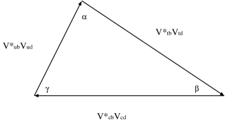
Figure 4: The KM unitarity triangle.

Among the six triangles defined by eq.(59), the one in Fig.4 will be experimentally studied in the near future. If $CP$ is conserved in the KM sector the triangle shrinks to a line. To test the KM mechanism for $CP$ violation it is sufficient to measure the three angles $\alpha$, $\beta$ and $\gamma$ and to see if they add up to $180^{o}$. Many methods have been proposed to determine these angles [34]. Alternatively one can also test the KM mechanism by measuring: 1) Two angles and one ratio of two sides of the triangle, for example, $|V_{ub}^{*}V_{ud}/V_{cb}^{*}V_{cd}|$; 2) One angle and two ratios for different two sides; and 3) Three ratios for different two sides.

3.1 The effective Hamiltonian for $B$ decays

In this section the effective Hamiltonian responsible for $B$ decays will be given. Both tree and loop contributions to $B$ decays are important. The Feynman diagrams for these decays up to one loop in electroweak interactions are shown in Fig.5.

Figure 5: The Feynman diagrams for $B$ decays up to one loop in electroweak interactions.

The effective Hamiltonian obtained from these diagrams with QCD corrections can be written as [35, 36]

$$H_{\Delta B=1}(q) ={4G_{F}\over\sqrt{2}}[V_{ub}V_{cq}^{*}(c_{1}O_{1}^{uc}(q)+c_{2}O_{2}^{uc}(q))$$ (60)

$$+V_{cb}V_{uq}^{*}(c_{1}O^{cu}_{1}(q)+c_{2}O^{cu}_{2}(q))+V_{ub}V^{*}_{uq}(c_{1}O^{u}_{1}(q)$$

$$+c_{2}O^{u}_{2}(q))+V_{cb}V^{*}_{cq}(c_{1}O^{c}_{1}(q)+c_{2}O^{c}_{2}(q))$$

$$-\sum_{j=u,c,t}V_{jb}V^{*}_{jq}\sum_{i=3}^{10}c_{i}^{j}O_{i}(q)]+H.C.,$$

where $O_{i}$’s are defined as

$$O^{f_{1}f_{2}}_{1}(q)=\bar{q}_{\alpha}\gamma_{\mu}Lf_{1\beta}\bar{f}_{2\beta}\gamma^{\mu}Lb_{\alpha},\ \ O^{f_{1}f_{2}}_{2}(q)=\bar{q}\gamma_{\mu}Lf_{1}\bar{f}_{2}\gamma^{\mu}Lb,$$

$$O^{f}_{1}(q)=\bar{q}_{\alpha}\gamma_{\mu}Lf_{\beta}\bar{f}_{\beta}\gamma^{\mu}Lb_{\alpha},\ \ O^{f}_{2}(q)=\bar{q}\gamma_{\mu}Lf\bar{f}\gamma^{\mu}Lb,$$ (61)

$$O_{3(5)}(q)=\bar{q}\gamma_{\mu}Lb\bar{q}^{\prime}\gamma^{\mu}L(R)q^{\prime},\ \ O_{4(6)}(q)=\bar{q}_{\alpha}\gamma_{\mu}Lb_{\beta}\bar{q}^{\prime}_{\beta}\gamma^{\mu}L(R)q^{\prime}_{\alpha},$$

$$O_{7(9)}(q)={3\over 2}\bar{q}\gamma_{\mu}Lbe_{q^{\prime}}\bar{q}^{\prime}\gamma^{\mu}R(L)q^{\prime},\ \ O_{8(10)}(q)={3\over 2}\bar{q}_{\alpha}\gamma_{\mu}Lb_{\beta}e_{q^{\prime}}\bar{q}^{\prime}_{\beta}\gamma^{\mu}R(L)q^{\prime}_{\alpha},$$

where $f$ can be $u$ or $c$ quark, $q$ can be $d$ or $s$ quark, and $q^{\prime}$ is summed over $u$, $d$, $s$, and $c$ quarks. $\alpha$ and $\beta$ are the color indices. $T^{a}$ is the SU(3) generator with the normalisation $Tr(T^{a}T^{b})=\delta^{ab}/2$. $G^{\mu\nu}_{a}$ and $F_{\mu\nu}$ are the gluon and photon field strengths, respectively. $c_{i}$ are the Wilson Coefficients (WC). The next-to-leading order QCD corrected WC’s with $\alpha_{s}(m_{Z})=0.118$, $\alpha_{em}(m_{Z})=1/128$, $m_{t}=176$ GeV and $\mu\approx m_{b}=5$ GeV, are given by [36]

$$c_{1} = -0.3125,\ \ c_{2}=1.1502,\ \ c_{3}^{t}=0.0174,\ \ c_{4}^{t}=-0.0373,$$

$$c_{5}^{t} = 0.0104,\ \ c_{6}^{t}=-0.0459,\ \ c_{7}^{t}=-1.050\times 10^{-5},$$

$$c_{8}^{t} = 3.839\times 10^{-4},\ \ c_{9}^{t}=-0.0101,\ \ c_{10}^{t}=1.959\times 10^{-3}\;,$$

$$c_{3,5}^{u,c} = -c_{4,6}^{u,c}/N_{c}=P_{s}^{u,c}/N_{c}\;,c_{7,9}^{u,c}=P_{em}^{u,c}\;,\;\;c_{8,10}^{u,c}=0\;,$$ (62)

where $N_{c}$ is the number of color, $P_{s}^{i}=(\alpha_{s}/8\pi)c_{2}[10/9+G(m_{i},\mu,q^{2})]$, and $P_{em}^{i}=\alpha_{em}/9\pi)(N_{c}c_{1}+c_{2})[10/9+G(m_{i},\mu,q^{2})]$. The function $G(m,\mu,q^{2})=4\int^{1}_{0}x(1-x)ln[(m^{2}-x(1-x)q^{2})/\mu^{2}]dx$.

One expects that the hadronic matrix elements arising from quark operator $O_{1-10}$ to be the same order of magnitudes. The relevant strengths of the contribution from each term in $H_{eff}$ are predominantly determined by their corresponding KM factors and the WC’s. This will provide guidance to identify dominant contribution for a decay process.

3.2 The determination of the angle $\alpha$

At asymmetric $B$ factories it is possible to measure the time variation of rate asymmetries of $B$ and $\bar{B}$. This provides an excellent opportunity to determine some of the angles [37, 38]. As an example let me first consider the standard method to measure $\alpha$ in $B\rightarrow\pi\pi$ [39, 40]. The time-dependent rate for initially pure $B^{0}$ or $\bar{B}^{0}$ to decay into a final CP eigenstate, for example $\pi^{+}\pi^{-}$ at time $t$ is [39]

$$\Gamma(t) = |A|^{2}e^{-\Gamma t}[{1+|\xi|^{2}\over 2}+{1-|\xi|^{2}\over 2}\cos{(\Delta Mt)}-Im\xi\sin{(\Delta Mt)}],$$

$$\bar{\Gamma}(t) = |A|^{2}e^{-\Gamma t}[{1+|\xi|^{2}\over 2}-{1-|\xi|^{2}\over 2}\cos{(\Delta Mt)}+Im\xi\sin{(\Delta Mt)}],$$ (63)

where $\xi$ is defined as

$$\xi=\left({q\over p}\right)_{B_{d}}{\bar{A}\over A}\;,$$ (64)

with $A=A(B^{0}\rightarrow\pi^{+}\pi^{-})$ and $\bar{A}=\bar{A}(\bar{B}^{0}\rightarrow\pi^{+}\pi^{-})$. Here $p$ and $q$ are given by

$$|B_{L,H}>=p|B^{0}>\pm q|\bar{B}^{0}>\;,$$ (65)

where $B_{H}$ and $B_{L}$ are the light and heavy mass eigenstates, respectively. In the SM $B^{0}-\bar{B}^{0}$ mixing is dominated by the top quark in the loop, and therefore

$$\left({q\over p}\right)_{B_{d}}={V_{tb}^{*}V_{td}\over V_{tb}V_{td}^{*}}\;.$$ (66)

The decay amplitude can, in general, be parametrized as

$$\bar{A}_{\pi^{+}\pi^{-}}=V_{ub}V_{ud}^{*}T_{\pi^{+}\pi^{-}}+V_{tb}V_{td}^{*}P_{\pi^{+}\pi^{-}}\;,$$ (67)

where the amplitude $T$ contains both tree and penguin contributions, and $P$ contains penguin contribution only. If the penguin amplitude $P_{\pi^{+}\pi^{-}}$ can be neglected, then

$$Im\xi=Im({V_{tb}^{*}V_{td}\over V_{tb}V_{td}^{*}}{V_{ub}V_{ud}^{*}\over V_{ub}^{*}V_{ud}})=\sin(2\alpha)\;.$$ (68)

The angle $\alpha$ can therefore be determined. However, if penguin effects are significant, the above method fails.

The decay $\bar{B}^{0}\rightarrow\pi^{+}\pi^{-}$ is induced by the effective Hamiltonian $H_{\Delta B=1}(d)$, and can be written as

$$T_{\pi^{+}\pi^{-}} = {4G_{F}\over\sqrt{2}}<\pi^{+}\pi^{-}|[c_{1}O^{u}_{1}(d)+c_{2}O^{u}_{2}(d))+\sum_{i=3}^{10}(c_{i}^{t}-c_{i}^{u})O_{i}(d)]|\bar{B}^{0}>$$

$$P_{\pi^{+}\pi^{-}} = {4G_{F}\over\sqrt{2}}\sum_{i=3}^{12}<\pi^{+}\pi^{-}|(c_{i}^{t}-c_{i}^{c})O_{i}(d)|\bar{B}^{0}>\;.$$ (69)

Since the KM factors $|V_{ub}V_{ud}^{*}|$ is the same order of magnitude compared with $|V_{cb}V_{cd}^{*}|$, the penguin contribution to the amplitudes are at the level of a few percent compared with the tree amplitudes. However, even such a small contribution may cause significant error in the determination of $\alpha$. It has been estimated [41] that the error can be as large as $12^{o}$. It is necessary to find ways to isolate the penguin contributions.

When penguin effects are included, the parameter $Im\xi$ for $\bar{B}^{0}\rightarrow\pi^{+}\pi^{-}$ becomes [40]

$$Im\xi={|\bar{A}|\over|A|}\sin(2\alpha+\theta)\;.$$ (70)

To determine $\theta$, Gronau and London[40] proposed to use isospin relation

$$\sqrt{2}\bar{A}(\bar{B}^{0}\rightarrow\pi^{0}\pi^{0})+\sqrt{2}\bar{A}(B^{-}\rightarrow\pi^{-}\pi^{0})=\bar{A}(\bar{B}^{0}\rightarrow\pi^{+}\pi^{-})\;,$$ (71)

and similar relation for the $CP$-conjugate amplitudes for the corresponding anti-particle decays. If all the six amplitudes can be measured, the angle $\theta$ can be determined up to two fold ambiguity as shown in Fig.6. This is a very interesting theoretical idea. Experimentally, it may be difficult to measure $\theta$ accurately because the branching ratio for $\bar{B}^{0}\rightarrow\pi^{0}\pi^{0}$ is expected to be of order $O(10^{-6})$. It has been pointed out that measurements for amplitude differences in $B\rightarrow\pi K$ may help the measurements in $B\rightarrow\pi\pi$ and improve the situation [42].

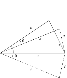
Figure 6: Isospin triangles in the complex plane. Lines $a$, $b$, and $c$ denote the amplitudes $\bar{A}(B^{0}\rightarrow\pi^{+}\pi^{-})$, $\sqrt{2}\bar{A}(B^{-}\rightarrow\pi^{-}\pi^{0})=\sqrt{2}A(B^{+}\rightarrow\pi^{+}\pi^{0})$, and $\sqrt{2}\bar{A}(B^{0}\rightarrow\pi^{0}\pi^{0})$,respectively. The dashed lines $d$ and $e$ (or $d^{\prime}$ and $e^{\prime}$) denote the amplitudes $A(B^{0}\rightarrow\pi^{+}\pi^{-})$ and $\sqrt{2}A(B^{0}\rightarrow\pi^{0}\pi^{0})$, respectively.

$\bar{B}^{0}\rightarrow\pi\rho$ are induced by the same effective Hamiltonian. Similarly the penguin contamination can be removed by isospin analysis. These decay modes also provide a measurement for $\alpha$ [43]. Combining this measurement with that from $B\rightarrow\pi\pi$, the two fold ambiguity mentioned above can be eliminated.

3.3 The determination of the angle $\beta$

The best way to determine $\beta$ is to measure $Im\xi$ for $\bar{B}^{0}(B^{0})\rightarrow J/\psi K_{S}$ [39]. The decay amplitude can be parameterized as

$$A(\bar{B}^{0}\rightarrow J/\psi K_{S})=V_{cb}V_{cs}^{*}T_{\psi K}+V_{ub}V_{us}^{*}P_{\psi K}\;.$$ (72)

The WC’s involved indicate that $|T_{\psi K}|$ is much larger than $|P_{\psi K}|$. Also $|V_{cb}V_{cs}^{*}|$ is about 50 times larger than $|V_{ub}V_{us}^{*}|$ from experimental data. One can safely neglect the contribution from the term proportional to $V_{ub}V_{us}^{*}$. To a very good approximation,

$$Im\xi=Im\left(\left({q\over p}\right)_{B_{d}}{V_{cb}V_{cs}^{*}\over V_{cb}^{*}V_{cs}}\left({q\over p}\right)_{K}\right)=-\sin(2\beta)\;.$$ (73)

Here $(q/p)_{K}$ is the mixing parameter for $K^{0}-\bar{K}^{0}$ which is given by $V_{cs}V_{cd}^{*}/V_{cs}^{*}V_{cd}^{*}$ and is small in the SM. $\beta$ can be measured accurately. This is the Gold-plated place to look for $CP$ violation.

3.4 The determination of the angle $\gamma$

The measurement of the angle $\gamma$ is an interest one. All methods proposed to measure $\gamma$ containing contributions from penguins involve additional assumptions about hadronic matrix elements which are subject to further improvement [44]. The best method to measure $\gamma$ is to use processes induced by the tree amplitudes for $b\rightarrow u\bar{c}s$ and $b\rightarrow c\bar{u}s$.

Let me give an example based on the measurements of [45] $B^{-}\rightarrow(D^{0},\;\bar{D}^{0},$ $D_{CP})K^{-}$. Here $D_{CP}=(D^{0}-\bar{D}^{0})/\sqrt{2}$ is the CP even state. The decay amplitudes can be parameterised as

$$\bar{A}(\bar{D}^{0}K^{-}) = V_{ub}V_{cs}^{*}T_{\bar{D}K}\;,\;\;\bar{A}(D^{0}K^{-})=V_{cb}V_{us}^{*}T_{D^{0}K}\;,$$

$$\bar{A}(D_{CP}K^{-}) = {1\over\sqrt{2}}(\bar{A}(D^{0}K^{-})-\bar{A}(\bar{D}^{0}K^{-}))\;.$$ (74)

The angle $\gamma$ can be measured as shown in Fig.7. The identification of $D_{CP}$ is through processes induced by $c\rightarrow ud\bar{d}$ and $\bar{c}\rightarrow\bar{u}\bar{d}d$. The angle $\gamma^{\prime}$ in Fig.7 is given by the absolute value of $\mbox{Arg}[(V_{ub}V_{cs}^{*}/V_{cb}V_{us}^{*})(V_{cd}V_{ud}^{*}/V_{cd}^{*}V_{ud})]=-2(\gamma-\sigma^{\prime})$. In the SM $\sigma^{\prime}$ is very small, so $\gamma^{\prime}$ is equal to $2\gamma$ to a very good approximation. There is a two-fold ambiguity in the determination of $\gamma$ as shown in Fig.7. This ambiguity can be eliminated when combined with other measurements like, $B^{-}\rightarrow DK^{*-}$ and other similar decays [46].

Figure 7: The measurement of $\gamma$ through $B^{-}(B^{+})\rightarrow DK^{-}(K^{+})$ decays with $a=|\bar{A}(B^{-}\rightarrow D^{0}K^{-})|=|A(B^{+}\rightarrow\bar{D}^{0}K^{+})|$, $b=\bar{A}(B^{-}\rightarrow\bar{D}^{0})$, $\bar{b}=A(B^{+}\rightarrow D^{0}K^{+})$, $c=\sqrt{2}\bar{A}(B^{-}\rightarrow D_{CP}K^{-})$, and $\bar{c}=\sqrt{2}A(B^{+}\rightarrow D_{CP}K^{+})$.

3.5 Other ways of testing the SM for $CP$ violation

The error on the measurement of $|V_{ub}/V_{cb}|$ may well be under control. One can measure this ratio and two other phase angles to test the SM [47]. In fact this may be a more convenient way to measure $CP$ violation in the KM sector in the presence of new source for $CP$ violation which I will return to later.

It is very optimistic that the SM for $CP$ violation will be tested at $B$ factories.

4 Models For $CP$ Violation

There are many other models for CP violation. In the following two representative models will be discussed. One is $CP$ violation due to spontaneous symmetry breaking [13, 14] and another $CP$ violation due to right-handed charged current in Left-Right symmetric model [15]. These two types of models have interesting features. In the SM $CP$ is explicitly violated. In 1973 T.D. Lee first pointed out that $CP$ can actually be broken spontaneously [13]. This opened a new direction in the study of $CP$ violation [48]. Another interesting feature of CP violation in the SM is that it only appears in the left-handed charged current. It is not sensitive to the right-handed sector. However, this is changed in the Left-Right symmetric model because the existence of right-handed charged current [15]. $CP$ can be violated by phases in the right-handed charge current. In these models, it is not necessary to have at least three generations to violate $CP$.

4.1 Spontaneous $CP$ violation

The basic idea for spontaneous $CP$ violation is best illustrated by using a toy model given by T.D. Lee. The Lagrangian for this model is [13]

$$L = -{1\over 2}\partial_{\mu}\phi\partial^{\mu}\phi-V(\phi)$$ (75)

$$- {i\over 2}(\bar{\psi}\gamma_{\mu}\partial^{\mu}\psi-\partial^{\mu}\bar{\psi}\gamma_{\mu}\psi)+m\bar{\psi}\psi-ig\bar{\psi}\gamma_{5}\psi\phi\;,$$

where $\phi$ is a pseudoscalar field and $\psi$ is a spinor, $V(\phi)$ is the potential for $\phi$ field. It is given by

$$V(\phi)={1\over 8}k^{2}(\phi^{2}-v^{2})^{2}\;.$$ (76)

The transformation properties of $\phi$ under $P$, $C$ and $T$ are:

$$P\phi=-\phi\;,\;\;C\phi=\phi\;,\;\;T\phi=-\phi\;.$$ (77)

The spinor has the usual transformation properties. If the $\phi$ field does not develop any VEV, that is, $<\phi>=0$, the above model is invariant under $CP$ transformation. However, the zero VEV for $\phi$ is not the minimal of the potential. The minimal occurs at $<\phi>=\pm v$ as shown in Fig.8. In the broken phase (in the phase with $<\phi>=v$, for example), the Lagrangian is given by,

$$L = -{1\over 2}\partial_{\mu}H\partial^{\mu}H-V(H)$$

$$- {i\over 2}(\bar{\psi}\gamma_{\mu}\partial^{\mu}\psi-\partial^{\mu}\bar{\psi}\gamma_{\mu}\psi)+m\bar{\psi}\psi-igv\bar{\psi}\gamma_{5}\psi-ig\bar{\psi}\gamma_{5}\psi H\;,$$

$$V(H) = {1\over 8}k^{2}(H^{2}+2vH)^{2}\;.$$ (78)

Here the field $H$ is defined as $\phi=v+H$ which has the same $C$, $P$ and $T$ transformation properties as $\phi$ in the unbroken phase. The VEV $v$ is a constant which does not transform under $P$, $C$ and $T$. The potential $V(H)$ under $CP$ transformation becomes: $V^{CP}(H)=(1/8)k^{2}(H^{2}-2vH)^{2}$, and the term $igv\bar{\psi}\gamma_{5}\psi$ changes sign under $CP$. $CP$ is spontaneously broken in the model. It is violated both in the scalar potential and in the scalar-fermion interaction sectors.

$CP$ violation in the scalar-fermion interaction sector is more transparent if one works in the fermion mass eigenstate basis where the mass is a real number. This can be achieved by a chiral rotation on the fermion, $\psi^{\prime}=exp(i\alpha\gamma_{5}/2)\psi$ with $tan(\alpha)=gv/m$. In this basis, the kinetic energy term has the same form as in the $\psi$ basis, but the mass and fermion-scalar interaction terms will be changed. One has

$$L(\psi^{\prime})=\sqrt{m^{2}+g^{2}v^{2}}\bar{\psi}^{\prime}\psi^{\prime}-g\bar{\psi}^{\prime}(i\gamma_{5}cos\alpha-sin\alpha)\psi^{\prime}H+...\;.$$ (79)

The $H$ field has both scalar and pseudoscalar couplings to the fermion $\psi^{\prime}$. Exchange of $H$ between fermions violates $CP$.

Figure 8: The potential for the $\phi$ field.

In the SM it is not possible to have spontaneous $CP$ violation. It requires at least two Higgs doublets to have a realistic model. With two Higgs doublets $H_{1}$ and $H_{2}$ transforming as $(1,2,-1)$ under the SM gauge group, the most general Higgs potential one can write is [13]:

$$V(H_{1},H_{2}) = \mu^{2}_{i}H^{\dagger}_{i}H_{j}+\lambda_{i}(H_{i}^{\dagger}H_{i})^{2}+\lambda^{\prime}_{i}(H_{i}^{\dagger}H_{j})(H_{j}^{\dagger}H_{i})$$ (80)

$$+ [\delta_{1}(H^{\dagger}_{1}H_{2})(H^{\dagger}_{1}H_{2})+\delta_{2}(H^{\dagger}_{1}H_{2})(H^{\dagger}_{1}H_{1})$$

$$+ \delta_{3}(H^{\dagger}_{1}H_{2})(H_{2}^{\dagger}H_{2})+H.C.]\;.$$

This potential only exhibits two possible electric charge conserving minimal characterised by the VEV’s, $<H_{i}>=v_{i}exp(i\theta_{i})$, and classified according to the value of the relative angle $\theta=\theta_{1}-\theta_{2}$ [49]:

$$\theta = 0\;\;\;\;\;\mbox{if}\;\;\delta_{1}<0\;,$$

$$\theta = arccos\left({\delta_{2}v_{1}^{2}+\delta_{3}v_{2}^{2}\over 4\delta_{1}v_{1}v_{2}}\right)\;\;\mbox{if}\;\;\delta_{1}>0\;.$$ (81)

The solution with $\theta=0$ does not violate $CP$, but the other one does.

Since $H_{1,2}$ have the same gauge transformation properties, their couplings to quarks are similar. The most general Yukawa interactions are given by

$$L_{Y}=\bar{Q}_{L}(\lambda_{1}^{U}H_{1}+\lambda_{2}^{U}H_{2})U_{R}+\bar{Q}_{L}(\lambda_{1}^{D}\tilde{H}_{1}+\lambda_{2}^{D}\tilde{H}_{2})D_{R}+H.C.$$ (82)

Figure 9: Flavour changing neutral current at tree level.

In this model there are three physical neutral Higgs and two charged Higgs particles. In general the neutral Higgs particles have flavour changing interactions at the tree level if $\lambda_{1}^{U,(D)}$ and $\lambda_{2}^{U,(D)}$ are not proportional [49, 50, 51, 52]. In fact there is no reason why they should be proportional. These flavour changing neutral current will induce $K^{0}-\bar{K}^{0}$ mixing at the tree level through the diagram shown in Fig.9. The Higgs particles are constrained to be very heavy [49, 50, 52]. There are rich phenomena related to $CP$ violation in this model [50, 52] which will not be discussed any further. Instead I will consider models which do not have tree level flavour changing neutral currents. This can be achieved if additional symmetries are imposed on the model such that only one of the Higgs doublets couples to each of the up, down quarks and the charged leptons.

If the additional symmetry is imposed on the entire model with two Higgs doublets, the parameter $\delta_{i}$ must all be zero if the vacuum state of the Higgs potential is at the minimal. There is no solution for spontaneous $CP$ violation. In order to achieve spontaneous $CP$ violation, at least three Higgs doublets are needed. A minimal model is the Weinberg model [14]. In this model there are three Higgs doublets $H_{1,2,3}$. The following is a set of possible discrete symmetries $D_{1}$ and $D_{2}$ which can achieve the goal [53],

$$D_{1}:Q_{L}\rightarrow Q_{L}\;,\;\;U_{R}\rightarrow U_{R}\;;\;\;D_{R}\rightarrow-D_{R}\;,\;\;H_{2}\rightarrow-H_{2}\;,\;\;H_{1,3}\rightarrow H_{1,3}\;.$$

$$D_{2}:Q_{L}\rightarrow Q_{L}\;,\;\;U_{R}\rightarrow U_{R}\;,\;\;D_{R}\rightarrow D_{R}\;,\;\;H_{1,2}\rightarrow H_{1,2}\;,\;\;H_{3}\rightarrow-H_{3}\;.$$

The Higgs potential is given by

$$V(H_{i}) = \mu^{2}_{i}(H_{i}^{\dagger}H_{i})+\delta_{i}(H^{\dagger}_{i}H_{i})^{2}+\delta^{\prime}_{ij}(H_{i}^{\dagger}H_{j})(H^{\dagger}_{j}H_{i})$$ (84)

$$+ \delta_{12}(H_{1}^{\dagger}H_{2})(H^{\dagger}_{1}H_{2})+\delta_{13}(H_{1}^{\dagger}H_{3})(H_{1}^{\dagger}H_{3})$$

$$+ \delta_{23}(H_{2}^{\dagger}H_{3})(H_{2}^{\dagger}H_{3})+H.C.,$$

and the Yukawa interaction for quarks are given by

$$L_{Y}=Q_{L}\lambda^{U}H_{1}U_{R}+\bar{Q}_{L}\lambda^{D}\tilde{H}_{2}D_{R}+H.C.$$ (85)

If all the constants in the Higgs potential and in the Yukawa interaction are real, there is no explicit $CP$ violation. After symmetry breaking the situation is changed . The VEV’s of the Higgs doublets can develop relative phases, $<H_{i}>=exp(i\theta_{i})$, if $\lambda_{12}\lambda_{13}\lambda_{23}\neq 0$. Minimising the Higgs potential one obtains

$$C_{CP}=\lambda_{12}v_{1}v_{2}sin(\theta_{2}-\theta_{1})=\lambda_{13}v_{1}v_{3}sin(\theta_{3}-\theta_{1})=\lambda_{23}v_{2}v_{3}sin(\theta_{3}-\theta_{2})\;.$$ (86)

If $C_{CP}$ is not zero, $CP$ is violated.

In this model, there are five neutral Higgs and four charged Higgs particles. The couplings of these Higgs particles to quarks can be written as

$$L_{CC} = 2^{7/4}G_{F}^{1/2}\bar{U}[V_{KM}M_{D}(\alpha_{1}H_{1}^{+}+\alpha_{2}H_{2}^{+})R$$

$$+ M_{U}V_{KM}(\beta_{1}H_{1}^{+}+\beta_{2}H_{2}^{+})L]D+H.C.$$

$$L_{NC} = 2^{7/4}G_{F}^{1/2}\sum_{i}m_{i}\bar{q}_{i}(\sigma_{i}+i\rho_{i}\gamma_{5})q_{i}H_{i}^{0}\;,$$ (87)

where $q_{i}$ is one of the quarks. $V_{KM}$ is real because there is no explicit violation of $CP$. Because $C_{CP}$ is non-zero, $Im(\alpha_{1}\beta_{1})=Im(\alpha_{2}\beta_{2})$ and $\sigma_{i}\rho_{i}$ are non-zero [54]. These imply $CP$ violation in the Yukawa interactions.

In later discussions it will be assumed that all Higgs particles are heavy except one for each charged and neutral Higgs particles. They will be indicated by a subindex ”1”.

In this model $CP$ is also violated in the lepton sector through Yukawa couplings. There are different ways leptons can couple to Higgs particles. One of the possibilities is to assume that $H_{3}$ is the Higgs which couples to leptons. In this case the leptons transform under the discrete symmetry as

$$D_{1}: L_{L}\rightarrow L_{L}\;,\;\;E_{R}\rightarrow E_{R}\;;$$

$$D_{2}: L_{L}\rightarrow L_{L}\;,\;\;E_{R}\rightarrow-E_{R}\;.$$ (88)

Figure 10: The new ”box” diagrams in the Weinberg model.

The Weinberg model can easily explain the observed $CP$ violation in $K^{0}-\bar{K}^{0}$ mixing. Naively, one would expect that the $CP$ violating parameter $\epsilon$ is induced by the ”box” diagrams as shown in Fig. 10. This turned out to be problematic because the enhanced $\Delta S=1$ interaction, i.e., the gluon dipole penguin interaction shown in Fig.11,

$$L_{CP} = i{G_{F}\over\sqrt{2}}{g_{s}\over 32\pi^{2}}m_{s}\sum_{ij}x_{ij}(V_{id}^{*}V_{is})\bar{f}_{ij}\bar{d}\sigma_{\mu\nu}(1+\gamma_{5})\lambda^{a}sG_{a}^{\mu\nu}\;,$$

$$\bar{f}_{ij} = -Im(\alpha_{i}\beta^{*}_{i})[{1\over 2(1-x_{ij})}+{1\over(1-x_{ij})^{2}}+{1\over(1-x_{ij})^{3}}lnx_{ij}]\;,$$ (89)

where $x_{ij}=m_{j}^{2}/m_{H_{i}}$.

Figure 11: The strong dipole penguin diagram due to Higgs exchange in the Weinberg model.

If $\epsilon$ is purely due to the ”box” diagrams in Fig.10, the magnitude for the $CP$ violating parameter $\epsilon^{\prime}/\epsilon$ is predicted to be too large compared with experimental data [55]. However, it was pointed out [56, 57] that if $\epsilon$ is actually dominated by the long distance interaction as shown in Fig.12, the problem can be solved. The $CP$ violating part of $M_{12}$ is given by [57],

$$Im(M_{12}) = {1\over 4m_{K}}\sum_{i=\pi,\eta,\eta^{\prime}}{Im(<K^{0}|L|i><i|L|\bar{K}^{0}>)\over m_{K}^{2}-m_{i}^{2}}$$

$$= {2\kappa\over m_{K}^{2}-m_{\pi}^{2}}<K^{0}|L_{CP}|\pi^{0}><\pi^{0}|L|\bar{K}^{0}>\;.$$

$$\kappa = 1+{m_{K}^{2}-m_{\pi}^{2}\over m_{K}^{2}-m_{\eta}^{2}}(\sqrt{{1\over 3}}(1+\delta)cos\theta+2\sqrt{{2\over 3}}\rho sin\theta)^{2}$$ (90)

$$+ {m_{K}^{2}-m_{\pi}^{2}\over m_{K}^{2}-m_{\eta^{\prime}}^{2}}(\sqrt{{1\over 3}}sin\theta-2\sqrt{{2\over 3}}\rho cos\theta)^{2}\;,$$

where [58] $\theta\approx-20^{o}$ is the $\eta-\eta^{\prime}$ mixing angle, $\delta=0.17$ and $\rho=0.75\pm 0.05$ parameterize flavour symmetry breakings,

$$<\eta_{8}|L|K^{0}> = \sqrt{{1\over 3}}(1+\delta)<\pi^{0}|L|K^{0}>\;,$$

$$<\eta_{0}|L|K^{0}> = -2\sqrt{{2\over 3}}\rho<\pi^{0}|L|K^{0}>\;.$$ (91)

Using the facts that due to mass suppression factor for the $u$ quark in the loop and KM suppression factor for $t$ in the loop, the dominant contribution is from $c$ quark in the loop [57], one obtains

$$4m_{K}Im(M_{12})=-4.3\times 10^{-16}\bar{f}_{1c}\;GeV^{2}\;,$$ (92)

and the function $\bar{f}_{1c}$ is determined to be $(0.054\sim 0.061)$ GeV^-2, a reasonable value to have.

Figure 12: The dominant contribution to $\epsilon$ in the Weinberg model. The cross indicates a $CP$ violating weak vertex and the square indicates a $CP$ conserving weak vertex.

At this point I would like to point out that if one abandons the requirement of spontaneous $CP$ violation, it is possible to have $CP$ violation in both the KM and the Higgs sectors. Such models will have more flexibility to accommodate experimental data.

4.2 Left-Right Symmetric Model

The gauge group of the Left-Right symmetric model is $SU(3)_{C}\times SU(2)_{L}\times SU(2)_{R}\times U(1)_{B-L}$ [15, 59]. This model offers a possible explanation of why the observed weak charged current interactions are all left-handed, but not right-handed. In this model there are both left-handed and right-handed charged currents. The answer to the question asked is that spontaneous symmetry breaking first breaks the $SU(2)_{R}\times U(1)_{B-L}$ at a higher energy scale to $SU(3)_{C}\times SU(2)_{L}\times U(1)_{Y}$. Because the interaction strength is inversely proportional to the square of the energy scale, the right-handed current effects are suppressed. However, the appearance of right-handed current introduces non-negligible effects for $CP$ violation.

In Left-Right symmetric model the right-handed fermions are grouped into doublets under $SU(2)_{R}$. For the leptons, this requires the introduction of right-handed neutrino. The gauge group transformation properties of the fermions are:

$$Q_{L}:(3,2,1,1/3)\;,\;\; Q_{R}:(3,1,2,1/3)\;,$$

$$L_{L}:(1,2,1,-1)\;,\;\; L_{R}:(1,1,2,-1)\;.$$ (93)

Neutrinos are massive in this model. Depending on whether neutrinos have only dirac masses or have both dirac and majorana masses, the separation of the breaking scales for $SU(2)_{R}$ and $SU(2)_{L}$ can be achieved differently.

If neutrinos have dirac masses only, the desired symmetry breaking pattern can be achieved by introducing [59]

$$H_{L}:(1,2,1,1)\;,\;\;H_{R}:(1,1,2,1)\;,$$ (94)

with $<H_{R}>=v_{R}$ to be much larger than $<H_{L}>=v_{L}$. Therefore $SU(2)_{R}$ is broken at a larger energy scale than the one for $SU(2)_{L}$ breaking. Whereas if neutrinos have both dirac and mjorana masses, the desired symmetry breaking can be achieved by [59]

$$\Delta_{L}:(1,3,1,2)\;,\;\;\Delta_{R}:(1,1,3,2)\;,$$ (95)

with $<\Delta_{R}>=v_{R}$ much larger than $<\Delta_{L}>=v_{L}$.

To generate fermion masses, it is necessary to introduce Higgs bi-doublet

$$\phi:(1,2,2,0)=\left(\begin{array}[]{ll}\phi_{1}^{0}&\phi_{1}^{+}\\ \phi_{2}^{-}&\phi_{2}^{0}\end{array}\right)\;.$$ (98)

There are left-handed as well as right-handed charged currents in this model. They are

$$L_{CC}={1\over\sqrt{2}}(g_{L}\bar{U}\gamma^{\mu}LDW^{+}_{L\mu}+g_{R}\bar{U}\gamma^{\mu}RDW^{+}_{R\mu})\;,$$ (99)

where $g_{L}$ and $g_{R}$ are the gauge couplings for $SU(2)_{L}$ and $SU(2)_{R}$, respectively.

Because the VEV’s of $\phi$ break both $SU(2)_{R}$ and $SU(2)_{L}$, there is mixing between $W_{R}$ and $W_{L}$. The mass eigenstates $W_{1}$ and $W_{2}$ are related to the weak eigenstates by

$$\left(\begin{array}[]{l}W_{1}\\ W_{2}\end{array}\right)=\left(\begin{array}[]{ll}cos\xi&\sin\xi\\ -sin\xi&cos\xi\end{array}\right)\left(\begin{array}[]{l}W_{L}\\ W_{R}\end{array}\right)\;.$$ (106)

Writing the charged current interactions in the gauge boson mass eigenstate as well as the quark mass eigenstate basis, the charged currents become,

$$L_{CC} ={1\over\sqrt{2}}(g_{L}\bar{U}V_{KM}^{L}\gamma_{\mu}LDcos\xi+g_{R}\bar{U}V_{KM}^{R}\gamma_{\mu}RDsin\xi)W_{1}^{\mu}$$ (107)

$$+{1\over\sqrt{2}}(g_{R}\bar{U}V_{KM}^{R}\gamma^{\mu}RDcos\xi-g_{L}\bar{U}V_{KM}^{L}\gamma_{\mu}LDsin\xi)W_{2}^{\mu}+H.C.$$

where $V_{KM}^{L,R}$ are the equivalent $KM$ matrices for the left-handed and right-handed charged currents. Just like in the SM one can always absorb $2N-1$ parameters in the $KM$ matrix by redefining quark phases, one can choose a basis such that $V_{KM}^{L}$ is the same as in the SM. However, after this choice is made, there is no freedom to absorb parameters in $V_{KM}^{R}$. There are $N(N+1)/2$ phases in $V_{KM}^{R}$. $CP$ symmetry can be violated even with just one generation.

The observed $CP$ violation in $K^{0}-\bar{K}^{0}$ mixing can be easily accommodated. An interesting scenario is that mxings only occur among the first two generations. In this case $V_{KM}^{L}$ is real. $CP$ violating phases only exist in $V_{KM}^{R}$. There are three $CP$ violating phases appearing in $V_{ij}^{R}$, it can be parameterized as

$$V_{KM}^{R}=e^{i\gamma}\left(\begin{array}[]{ll}e^{-i\delta_{2}}cos\theta^{R}&e^{-i\delta_{1}}sin\theta^{R}\\ -e^{i\delta_{1}}sin\theta^{R}&e^{i\delta_{2}}cos\theta^{R}\end{array}\right)\;.$$ (110)

Because there is no $CP$ violation in the purely left-handed current interaction, right-handed charged current must provide the needed source for $CP$ violation. The dominant contribution is from the diagrams shown in Fig.13. Assuming $g_{L}=g_{R}$ and $|V{ij}^{L}|=|V_{ij}^{R}|$, one obtains

$$\epsilon={1\over 2\sqrt{2}}430{m_{W_{1}}^{2}\over m^{2}_{W_{2}}}sin(\delta_{2}-\delta_{1})e^{i\pi/4}\;.$$ (111)

Figure 13: The dominant contribution to $CP$ violation in $K^{0}-\bar{K}^{0}$ mixing to $\epsilon$ in the Left-Right symmetric model with two generation mixing.

There is constraints on the right-handed gauge boson mass from the mass difference between $K_{S}$ and $K_{L}$, $(m_{W_{1}}/m_{W_{2}})^{2}<1/430$ [60, 61]. This implies that the $CP$ violating parameter $|sin(\delta_{2}-\delta_{1})|$ must be larger than $2\sqrt{2}|\epsilon|$ [60, 61, 62].

5 The KM Unitarity Triangle And New Physics

In this section I discuss ways to extract variables in the KM matrix in the presence of new $CP$ violating sources. If new sources exist, such as in the Weinberg and Left-Rgiht symmetric models, the interpretation of the measurements discussed in Section 3 will have to be modified [47, 63, 64].

In general new CP violating interactions come in all possible ways. They can arise at the tree and/or loop levels. For a certain process there may be contributions from several different CP violating sources. It is important to isolate these sources. This is, of course, a very difficult task. In this section the possibility to achieve this task by using the $B$ decay modes discussed in Section 3, will be discussed.

If new CP violating interactions come at all stages, tree and loop, significantly, it is possible to see the deviation from the SM, but it is not possible to isolate individual contribution. However, in many models new CP violating contributions only have significant effects at loop levels in $B$ decays, like the Weinberg model. In the following I will concentrate on this class of models.

It has been point out in Section 3 that it is possible to determine the KM triangle by using just tree level processes, namely, $\gamma$ from $B^{-}\rightarrow DK^{-}$ and $|V_{ub}/V_{cb}|$ from $b\rightarrow u(c)l\bar{\nu}$. These two quantities will determine the shape of the unitarity triangle. ¿From these measurements, one knows for certain that if KM mechanism is, at least partially, responsible for CP violation. After this is done one can use the other processes to see what the new contributions are.

Quantities generated at loop level will have new $CP$ violating phases. The mixing parameters $(q/p)_{i}$ for $B^{0}-\bar{B}^{0}$, and $K^{0}-\bar{K}^{0}$ will be modified. They can be normalised to the SM ones as the following

$$\left({q\over p}\right)_{B_{d}}=\left({V_{tb}^{*}V_{td}\over V_{tb}V_{td}^{*}}\right)e^{2i\delta_{B_{d}}}\;,\;\;\left({q\over p}\right)_{K}=\left({V_{cd}^{*}V_{cs}\over V_{cd}V_{cs}^{*}}\right)e^{2i\delta_{K}}\;.$$ (112)

Because of the smallness of $\epsilon$, $\delta_{K}$ is negligibly small ($<10^{-3}$). Its contribution will be neglected.

The $B$ decay amplitudes involving loop corrections will also have new phases. They can be written in the following form

$$\bar{A}(\bar{B}^{0}\rightarrow\pi\pi) = V_{ub}V_{ud}^{*}e^{i\theta_{\pi\pi}}T_{\pi\pi}(new)\;,$$

$$\bar{A}(\bar{B}^{0}\rightarrow\psi K_{S}) = V_{cb}V_{cs}^{*}e^{i\theta_{\psi K}}T_{\psi K}(new)\;.$$ (113)

The measurements of $Im\xi$ for these processes will no longer have the clean interpretation as in the SM. One has

$$Im\xi_{\pi\pi} = Im\left(\left({q\over p}\right)_{B_{d}}{\bar{A}(\pi\pi)\over A(\pi\pi)}\right)$$

$$= \mbox{sin}[2(\alpha+\delta_{B}+\theta_{\pi\pi})]\;,$$

$$Im\xi_{\psi K} = Im\left(\left({q\over p}\right)_{B_{d}}\left({q\over p}\right)_{K}{\bar{A}(\psi K_{S})\over A(\psi K_{S})}\right)$$ (114)

$$= -\mbox{sin}[2(\beta-\delta_{B}-\theta_{\psi K})]\;.$$

If one also assumes that the loop contribution only has substantial contribution to $\delta_{B}$ and use $B\rightarrow\pi\pi$, $B\rightarrow J/\psi K_{S}$ and $B\rightarrow K^{-}(D^{0},\;\bar{D}^{0},\;D_{CP})$ as tests for the SM, one would still obtain the summation of the angles measured to be $180^{o}$ because $B\rightarrow\pi\pi$ would measure $\alpha+\delta_{B}$, $B\rightarrow J/\psi K_{S}$ would measure $\beta-\delta_{B}$ and $B\rightarrow K^{-}(D^{0},\;\bar{D}^{0},\;D_{CP})$ would still measure $\gamma$. One would not be able to know if new physics has shown up. However, if one supplements the measurement of $V_{ub}/V_{cb}$, and use the measurements of $\gamma$ and $V_{ub}/V_{cb}$ to fix the KM unitarity triangle first and the additional measurements from $B\rightarrow\pi\pi$ and $B\rightarrow J/\psi K_{S}$ will provide information about new physics.

Let me consider the Weinberg model in more detail [64] and assume that $CP$ violation appears in both the KM and Higgs sectors simultaneously. The decay amplitudes due to exchange of charged Higgs at tree level will be proportional to $V_{fb}V_{f^{\prime}q}^{*}(m_{b}m_{f^{\prime}}/m_{H_{i}}^{2})\alpha_{i}\beta_{i}^{*}$. Therefore if a decay involves light quark, the amplitude will be suppressed. Similar arguments apply to semi-leptonic decays of b quark. It is clear that the measurement of $\gamma$ and $|V_{ub}/V_{cb}|$ will not be affected.

However, at one loop level if the internal quark masses are large, sizeable CP violating decay amplitude may be generated. The leading term is from the strong dipole penguin interaction, similar to the diagram in Fig.11 with top quark in the loop[65],

$$L_{DP} =V_{tb}V_{tq}^{*}\tilde{f}O_{11}\;,$$

$$\tilde{f} ={G_{F}\over 16\sqrt{2}}\sum_{i}^{2}\alpha^{*}_{i}\beta_{i}{m_{t}^{2}\over m_{H_{i}}^{2}-m_{t}^{2}}[{m_{H_{i}}^{4}\over(m_{H_{i}}^{2}-m_{t}^{2})^{2}}\mbox{ln}{m_{H_{i}}^{2}\over m_{t}^{2}}-{m_{H_{i}}^{2}\over m_{H_{i}}^{2}-m_{t}^{2}}-{1\over 2}]\;,$$

$$O_{11} ={g_{s}\over 32\pi^{2}}m_{b}\bar{s}\sigma_{\mu\nu}RT^{a}bG^{\mu\nu}_{a}\;.$$ (115)

This is not suppressed compared with the penguin contributions in the SM. There is also a similar contribution from the operator $O_{12}$. However the WC of this operator is suppressed by a factor of $\alpha_{em}/\alpha_{s}$ and its contribution can be neglected. The contribution from $O_{11}$ can be written as

$$\bar{A}_{final}(weinberg)=-(V_{ub}V_{uq}^{*}+V_{cb}V_{cq}^{*})a_{final}e^{i\alpha_{H}}\;,$$ (116)

where $\alpha_{H}$ is the phase in $\tilde{f}$ which is decay mode independent, and $a_{final}=|\tilde{f}|<final\;state|O_{11}|B>$ which is decay mode dependent. Due to this contribution, the phases $\theta_{i}$ defined in eq.(113) will not be zero.

The charged Higgs bosons also contribute to the mixing parameters $(q/p)_{i}$. These contributions have the same KM factors as the SM, but in principle have additional phase factors due to non-zero $Im(\alpha_{1}\beta^{*}_{1})$.

¿From the above discussions, one sees that even with new contributions to $B$ decay amplitudes, the measurements of $\gamma$ and $|V_{ub}/V_{cb}|$ using $B^{-}\rightarrow(D^{0},\;\bar{D}^{0},\;D_{CP})K^{-}$ and $b\rightarrow u(c)l\bar{\nu}$ will be true measurements of these quantities. CP violation due to KM mechanism can be isolated. It is not possible to use these two measurements to distinguish the SM and the Weinberg model. However, if one also measures $Im\xi$ for $B\rightarrow\pi\pi$ and $\bar{B}^{0}\rightarrow\psi K_{S}$, these two models can be distinguished because if the SM is correct, the angles $\alpha$ and $\beta$ are measured, whereas if the Weinberg model is correct, the quantities $\alpha+\delta_{B}$ and $\beta-\delta_{B}-\theta_{\psi K}$ are measured.

The Left-Right symmetric model will have completely different results. In two generation mixing case, there is no unitarity triangle to talk about. With three generations, even thought the left-handed current still has a unitarity triangle as in the SM one, due to the appearance of right-handed current, new physics will come significantly at both the tree and loop levels. In general it is not possible to isolate the left-handed current contribution.

6 Direct $CP$ Violation In Neutral Kaon System

There are many other experiments which can test $CP$ violation in kaon system. I now discuss direct $CP$ violation in $K\rightarrow\pi\pi$ decays. For this purpose, it is convenient to study the quantities $\eta_{+-}$ and $\eta_{00}$ defined as the following [66]

$$\eta_{+-}={A(K_{L}\rightarrow\pi^{+}\pi^{-})\over A(K_{S}\rightarrow\pi^{+}\pi^{-})}\;,\;\;\eta_{00}={A(K_{L}\rightarrow\pi^{0}\pi^{0})\over A(K_{S}\rightarrow\pi^{0}\pi^{0})}\;.$$ (117)

One can express the above quantities in terms of $K^{0}(\bar{K}^{0})\rightarrow\pi\pi$ isospin decay amplitudes,

$$A(K^{0}\rightarrow\pi^{+}\pi^{-}) = \sqrt{{2\over 3}}A_{0}e^{i\delta_{0}}+\sqrt{{1\over 3}}A_{2}e^{i\delta_{2}}\;,$$

$$A(K^{0}\rightarrow\pi^{0}\pi^{0}) = \sqrt{{1\over 3}}A_{0}e^{i\delta_{0}}-\sqrt{{2\over 3}}A_{2}e^{i\delta_{2}}\;,$$ (118)

where $A_{0}$ and $A_{2}$ are decay amplitudes for isospin $I=0$ and $I=2$ final two pion systems, respectively. $\delta_{i}$ are the strong final state rescattering phases (strong phase).

The corresponding anti-particle decay amplitudes are

$$A(\bar{K}^{0}\rightarrow\pi^{+}\pi^{-}) = -\sqrt{{2\over 3}}A_{0}^{*}e^{i\delta_{0}}-\sqrt{{1\over 3}}A_{2}^{*}e^{i\delta_{2}}\;,$$

$$A(\bar{K}^{0}\rightarrow\pi^{0}\pi^{0}) = -\sqrt{{1\over 3}}A_{0}^{*}e^{i\delta_{0}}+\sqrt{{2\over 3}}A_{2}^{*}e^{i\delta_{2}}\;.$$ (119)

One has

$$\eta_{+-} = \epsilon+i{ImA_{0}\over ReA_{0}}+e^{i(\pi/2+\delta_{2}-\delta_{0})}{ReA_{2}\over\sqrt{2}A_{2}}\left({ImA_{2}\over ReA_{2}}-{ImA_{0}\over ReA_{0}}\right)\;,$$

$$\eta_{00} = \epsilon+i{ImA_{0}\over ReA_{0}}-2e^{i(\pi/2+\delta_{2}-\delta_{0})}{ReA_{2}\over\sqrt{2}ReA_{0}}\left({ImA_{2}\over ReA_{2}}-{ImA_{0}\over A_{0}}\right)\;,$$ (120)

and the parameter $\epsilon^{\prime}$ mentioned previously is defined as

$$\epsilon^{\prime}={\eta_{+-}-\eta_{00}\over 3}={ReA_{2}\over\sqrt{2}ReA_{0}}\left({ImA_{2}\over ReA_{2}}-{ImA_{0}\over ReA_{0}}\right)\;.$$ (121)

The strong phases $\delta_{i}$ can be determined from phase shift analyses in $\pi-\pi$ scattering, and $\pi/2+\delta_{2}-\delta_{0}$ is found to be close to $\pi/4$. The requirement of $CPT$ symmetry implies that this phase is equal to the phase $\phi_{\epsilon}$ for $\epsilon$. In the literature the quantity $\epsilon^{\prime}/\epsilon$ is usually used.

Experimental measurement of this quantity is not conclusive. While the result of NA31 at CERN [67] with $\epsilon^{\prime}/\epsilon=(23\pm 7)\times 10^{-4}$ clearly indicates direct $CP$ violation, the value of E731 at Fermilab [68], $\epsilon^{\prime}/\epsilon=(7.4\pm 5.9)\times 10^{-4}$ is compatible with $CP$ conservation.

The measurement of $\epsilon^{\prime}/\epsilon$ provides important information in distinguishing superweak model and other models because superweak model predicts zero value for $\epsilon^{\prime}/\epsilon$. This measurement also provides constraints for other models. In the SM a non-zero value for $\epsilon^{\prime}$ is generated at one loop level similar to the diagrams for $B$ decays as shown in Fig.5. This has been studied extensively in the liturature [69, 70, 71, 72]. One feature particularly interesting is that both the strong and electroweak penguin effects are important [69, 70]. Without electroweak penguin contribution, $\epsilon^{\prime}/\epsilon$ is predicted to be larger than the experimental limit. When the electroweak penguin effect is included, the situation is changed because although electroweak penguin contribution to the $I=0$ amplitude is small, it contributes to $I=2$ amplitude with substantial value for $ImA_{2}/ReA_{2}$. This new contribution tends to cancel $\epsilon^{\prime}/\epsilon$ from the strong penguin. The final value is predicted to be in the range of [72] $(-1.2\sim 44)\times 10^{-4}$ which is consistent with present experimental limit.

In the spontaneous $CP$ violation model, the most significant operator contributing to $\epsilon^{\prime}$ is from eq.(89). If the experimental value for $\epsilon$ is purely from the ”box” diagram shown is Fig.10, the predicted value for $\epsilon^{\prime}/\epsilon$ due to contribution from eq.(89) will be much large than the experimental limit. This problem is solved if the long distance contribution dominates $\epsilon$ as discussed earlier. If one naively use the chiral realisation of $L_{CP}$ in eq.(89) for $K\rightarrow\pi\pi$ and take the direct diagram (a) in Fig.14, one would obtain a large $\epsilon^{\prime}/\epsilon$ which is in conflict with experimental data. However, it was pointed out that at the same order there is another diagram (b) in Fig.14 which cancels the contribution from (a) in Fig.14 [56]. The contribution for $\epsilon^{\prime}/\epsilon$ comes at higher order and is suppressed. The parameter $\epsilon^{\prime}/\epsilon$ is predicted to be [57]

$${\epsilon^{\prime}\over\epsilon}\approx 0.017D\;,$$ (122)

with $D=O((m^{2}_{\pi}\;\mbox{or}\;m^{2}_{K})/\Lambda^{2}_{\chi})$ being a chiral suppression factor which characterises cancellations discussed above. The value for $\epsilon^{\prime}/\epsilon$ is in the range of $(0.4\sim 6.0)\times 10^{-3}$ which is, again, consistent with present experimental limit.

Figure 14: Cancellation between diagrams in the Weinberg model. The cross indicates a weak vertex and the square indicates a strong vertex.

In the Left-Right symmetric model with two generation mixing, the dominant contribution to $\epsilon^{\prime}/\epsilon$ is due to $W_{L}-W_{R}$ mixing, one obtains [62]

$${\epsilon^{\prime}\over\epsilon}=276\mbox{tg}\xi[sin(\gamma-\delta_{2})+sin(\gamma-\delta_{1})-0.1(sin(\gamma+\delta_{2})+sin(\gamma+\delta_{1}))]\;,$$ (123)

which can easily accommodate experimental data.

New experiment at DA$\phi$NE will improve the measurement for $\epsilon^{\prime}/\epsilon$ considerably [73]. Models for $CP$ violation will be further constrained.

There are many other experiments studying $CP$ violation in kaon systems. They have been discussed in several excellent reviews [74]. I will not discuss them here. In the following sections I will discuss $CP$ violation in other systems.

7 The Electric Dipole Moment

The interaction potential of an electric dipole $\vec{D}$ in an external electric field $\vec{E}$ is proportional to $\vec{D}\cdot\vec{E}$. Classically the electric dipole moment (EDM) is given by $\vec{D}=\int d^{3}x\vec{x}\rho(\vec{x})$, where $\rho(\vec{x})$ is the electric charge density. In the case of an elementary particle, the only (pseudo) vector that characterises its state is the spin $\vec{S}$; hence $\vec{D}$ must be of the form $d\vec{S}$. Here $d$ is a proportional constant representing the size of the EDM. Under $P$ transformation $\vec{D}\rightarrow\vec{D}$, $\vec{E}\rightarrow-\vec{E}$, while under $T$ transformation, $\vec{D}\rightarrow-\vec{D}$ and $\vec{E}\rightarrow\vec{E}$. So the interaction $\vec{D}\cdot\vec{E}$ changes sign under $P$ and $T$ transformation. If $d$ is not zero, $P$ and $T$ are violated simultaneously. This is a direct test of time reversal symmetry. Due to the $CPT$ theorem, a non-zero value for $d$ also violates $CP$. The EDM of an elementary particle is of interest for both experimental [75, 76, 77, 78] and theoretical [79, 80, 81, 82] studies.

7.1 The neutron EDM

The neutron EDM has been of interest to physicists for a long time. The measurement of the neutron EDM started in 1950 by Purcel and Ramsey [75]. Although no positive result has been obtained, very impressive progress (several orders of magnitude) on the upper bound has been obtained. The present experimental upper bound for the neutron EDM $d$ is [76] $1.2\times 10^{-25}$ ecm. There are also many experiments measuring the EDM’s of other particle systems, like the electron [77] and atoms [78]. Stringent bounds have also been obtained [82].

There are different contributions to the neutron EDM. It can arise at the hadron level as well as at the quark level. At the quark level, it can come from the quark EDM $d_{q}$, the color dipole moment (CDM) $f_{q}$, and other complicated $CP$ violating operators composed of quarks and/or gluons. In the valance quark model, the contributions from $d_{q}$ and $f_{q}$ are given by

$$d(d_{q}) = {1\over 3}(4d_{d}-d_{u})\;,\;\;d(f_{q})={1\over 9}e(4f_{d}+3f_{u})\;.$$ (124)

For complicated operators it is very difficult, if not impossible, to calculate their contributions to the neutron EDM. In this case dimensional analysis may help to make an order of magnitude estimate. A commonly used nethod is the so called ”naive dimensional analysis” (NDA) [83] which keeps track of factors of $4\pi$ from loops and mass scales involved. Giving a $CP$ violating operator, $O$ with coefficient $C$, one defines the reduced coupling constant $(4\pi)^{2-N}\Lambda_{\chi}^{D-4}C$ where $\Lambda_{\chi}=2\pi f_{\pi}=1190MeV$ is the chiral symmetry breaking scale, $N$ is the number of fields and $D$ is the dimension of the operator. The neutron EDM operator has a reduced coupling $d_{n}\Lambda_{\chi}/4\pi$. For a $CP$ violating operator $O$ which does not involve photon, in order to produce a neutron EDM a photon has to be attached to a quark. This electromagnetic coupling of quark has a reduced coupling $e/4\pi$. So the NDA suggests that the neutron EDM due to the operator $O$ is given by,

$$d_{n}\approx{e\over\Lambda_{\chi}}(4\pi)^{2-N}\Lambda_{\chi}^{D-4}C.$$ (125)

Of course, one must keep in mind that this is only an order of magnitude estimate.

It has been shown that in the SM the quark EDMs are zero at one and two loop levels [84]. The neutron EDM is generated at three loop level and therefore is very small in size. A typical set of diagrams which generate neutron EDM with hadron loops is shown in Fig.15 [85]. The neutron EDM was estimated to be in the range of $10^{-31}\sim 10^{-33}$ ecm [79]. This is several orders of magnitude below the experimental upper bound.

Figure 15: Some typical diagrams generating the neutron EDM in the SM. Each cross indicates a weak vertex which is equivalent to a loop contribution.

In extensions of the SM because new sources for $CP$ violation, a non-zero neutron EDM can be generated at lower loop levels and therefore can be much larger than that in the SM. A measurement of the neutron EDM at a level larger than $10^{-31}$ ecm would indicate new sources for $CP$ violation.

In the Weinberg model a non-zero neutron EDM can be generated by exchanging Higgs particles. At one loop level (Fig.16), exchange of charged Higgs will generate quark EDM’s given by [48, 79]

$$d_{q}={G_{F}\over 6\sqrt{2}\pi^{2}}m_{q}Im(\alpha_{1}\beta_{1}^{*})\sum_{i}{x_{i}\over(1-x_{i})^{2}}({3\over 4}-{5\over 4}x_{i}+{1-3x_{i}/2\over 1-x_{i}}lnx_{i})V_{qi}^{2}\;,$$ (126)

for charge -1/3 quarks, and

$$d_{q}={G_{F}\over 6\sqrt{2}}m_{q}Im(\alpha_{1}\beta_{1}^{*})\sum_{i}{x_{i}\over(1-x_{i})^{2}}(x_{i}-{1\over 2}{1-3x_{i}\over 1-x_{i}}lnx_{i})V_{iq}^{2}\;.$$ (127)

for charge 2/3 Quarks, where $x_{i}=m_{i}^{2}/m_{H}^{2}$. It is easy to see that $d_{d}>>d_{u}$ and the dominant contribution to $d_{d}$ is due to c quark in the loop. Taking the value of $Im(\alpha_{1}\beta_{1})$ determined from eq. (92), the neutron EDM is found to be [48]

$$d\approx-9\times 10^{-26}ecm\;.$$ (128)

It is very close to the experimental upper bound. Improved measurement will provide decisive information about this model.

Figure 16: One loop contribution to the quark EDM in the Weinberg model.

The neutral Higgs contribution is predicted to be small because the quark EDM is proportional to the third power of the light quark masses. However, there are estimates which obtain larger contributions [86].

In the Weinberg model, the contribution from the two-loop diagrams shown in Fig.17 [87] contribution to neutron EDM may dominate over that from the one loop diagrams. The basic reason for a large EDM at two loop level is because Higgs couplings to fermions are proportional to fermion masses. At one loop level, the relevant fermions are the light fermions, u and d quark, but at two loop level, heavy fermions can be in the loop, for example, the top quark. The couplings are much larger which may overcome the suppression due to loop.

One of the typical $CP$ violating operator is

$$O=-{1\over 6}f_{\alpha\beta\gamma}G_{\alpha\mu\rho}G_{\beta\nu}^{\rho}G_{\gamma\lambda\sigma}\epsilon^{\mu\nu\lambda\sigma}\;.$$ (129)

Figure 17: Two loop diagram for gluon color dipole moment.

It is, of course, very difficult to calculate its contribution to the neutron EDM. The NDA estimate gives

$$d={e\over 4\pi}\Lambda_{\chi}C\;,$$ (130)

where $C$ is the coefficient of $O$.

The neutral Higgs contribution to $C$ is give by [87]

$$C=\xi(\mu){G_{F}\over 2\sqrt{2}}ImZ_{1}h(m^{2}_{t}/m_{H}^{2})\;,$$ (131)

where the function $h(x)$ is from the loop integral and is given by

$$h(x)={1\over 4}\left({m_{t}\over m_{H_{1}}}\right)^{4}\int^{1}_{0}dx\int^{1}_{0}{x^{3}y^{3}(1-x)\over((m_{t}/m_{H_{1}})^{2}x(1-xy)+(1-x)(1-y))^{2}}\;,$$ (132)

$\xi(\mu)$ is the QCD correction factor which is given by [88]

$$\xi(\mu)=\left({g_{s}(m_{b})\over g_{s}(m_{t})}\right)^{-18/\beta_{5}}\left({g_{s}(m_{c})\over g_{s}(m_{b})}\right)^{-18/\beta_{4}}\left({g_{s}(\mu)\over g_{s}(m_{c})}\right)^{-18/\beta_{3}}\;,$$ (133)

and $ImZ_{1}$ is the $CP$ violating parameter in the Higgs propagator which is proportional to $\delta_{1}\rho_{1}$.

Assuming $m_{t}\sim m_{H_{1}}$, and taking $g_{s}(\mu)=4\pi/\sqrt{6}$, one obtains

$$d\approx 4\times 10^{-26}ImZ_{1}ecm\;.$$ (134)

There is also charged Higgs contribution. It is given by [87]

$$d=4\times 10^{-24}Im(\alpha_{1}\beta^{*}_{1})h_{c}((m_{t}/m_{H_{1}})^{2})\;,$$ (135)

with

$$h_{c}(x)\approx{1\over 4}{x\over(1-x)^{3}}(-lnx-{3\over 2}+2x-{1\over 2}x^{2})\;.$$ (136)

If one uses the value for $Im(\alpha_{1}\beta_{1}^{*})$ from eq.(92) the neutron EDM is above the experimental upper bound. However, one must be very careful to draw conclusion that the Weinberg model is ruled out from this consideration. As has been pointed out previously that the NDA estimate is just an order of magnitude guess. A factor of ten can be easily missed. The above estimate may be just such a case.

At two loop level, there are several other contributions which can generate a neutron EDM close to the experimental upper limit [89, 90, 91]. Some of them are shown in Fig.18 [89, 90].

Figure 18: Additional two loop diagrams.

In the Left-Right symmetric model due to mixing between left-handed and right-handed charged currents, the quark EDM is generated at one loop level as shown in Fig. 19. One has [62, 92]

$$d \approx sin2\xi[4.5sin(\gamma-\delta_{2})+74sing(\gamma+\delta_{1})$$ (137)

$$-1.1sin(\gamma-\delta_{1})+16sin(\gamma+\delta_{2})]\times 10^{-23}ecm\;.$$

The neutron EDM from this contribution can be close to the experimental upper bound.

Figure 19: One loop diagrams for quark EDM in Left-Right symmetric model.

7.2 The Electron EDM

The best limit on the electron EDM $d_{e}$ is from the EDM measurement of ${}^{205}Tl$, and is given by [77]

$$d_{e}=[1.8\pm 1.2(stat.)\pm 1.0(sys.)]\times 10^{-27}ecm.$$ (138)

In the SM the electron EDM $d_{e}$ is zero at three loop level [93] and is predicted to be less than $10^{-38}$ ecm.

In the Weinberg model $d_{e}$ is generated at one loop level. However at this level, $d_{e}$ is proportional to the third power in the electron mass. $d_{e}$ is predicted to be very small ($10^{-33}ecm$). At two loop level, $d_{e}$ can be quite large due to the second diagram (b) in Fig.18 with quarks replaced by leptons in the diagram. $d_{e}$ can be close to the experimental bound  [89].

In the Left-Right symmetric model, $d_{e}$ is also generated at one loop level. It can be as large as $10^{-27}$ ecm [81].

The measurements of EDM’s of neutron and electron are very interesting measurements because in the SM the EDM’s for these particles are predicted to be very small. Any new measurements with improved sensitivity may reveal new source for $CP$ violation. In fact present upper bound provided very strong constraints on models as discussed before. There is a potential problem for the Weinberg model. Another interesting problem related to the neutron EDM measurement is the so called strong $CP$ problem. This problem will be briefly discussed in the following section.

7.3 The strong $CP$ problem

It has long been realised that due to instanton effects [94] in non-Abelian gauge theory, the total divergence term

$${1\over 2}\epsilon_{\mu\nu\alpha\beta}G^{\mu\nu}_{a}G_{\alpha\beta}^{a}=\tilde{G}_{a}^{\alpha\beta}G^{a}_{\alpha\beta}\;.$$ (139)

constructed from the field strength $G^{\mu\nu}_{a}$ has non-vanishing physical effects. The index ”a” is an internal group index. In the case of $QCD$, $G^{\mu\nu}_{a}$ is the gluon field strength. The full QCD Lagrangian is given by

$$L_{QCD}=-{1\over 4}G^{\mu\nu}_{a}G^{a}_{\mu\nu}+\bar{q}(D_{\mu}\gamma^{\mu}-m)q-\theta{g^{2}\over 32\pi^{2}}\tilde{G}^{\mu\nu}_{a}G_{\mu\nu}^{a}\;,$$ (140)

where q is the quark field, m is the quark mass, $D_{\mu}$ is the covariant derivative and $\theta$ is a constant.

The last term in $L_{QCD}$ violates $P$ and $CP$. This term will generate $CP$ violating nucleon-meson interaction at low energy. Using chiral realisation of this interaction, one obtains [95]

$$L_{\pi NN}=\sqrt{2}\bar{N}\vec{\pi}\cdot\vec{\tau}(i\gamma_{5}g_{\pi NN}+f_{\pi NN})N\;,$$

$$f_{\pi NN}=-{1\over\sqrt{2}}2(m_{\Xi}-m_{\Sigma}){m_{u}m_{d}m_{s}\over F_{\pi}(m_{u}+m_{d})(2m_{s}-m_{u}-m_{d})}\;.$$ (141)

Here $g_{\pi NN}^{2}/4\pi\approx 14$ is the $CP$ conserving strong nucleon-meson coupling constant, and $F_{\pi}=93$ MeV is the pion decay constant. At one loop level a non-zero neutron EDM is generated. The result obtained from the Feynman diagrams in Fig.20 is [95]

$$d=-3.8\times 10^{-16}\theta\mbox{ecm}\;.$$ (142)

And the full one loop result is given by [79]

$$2.5\times 10^{-16}\theta\mbox{ecm}<|d|<4.6\times 10^{-16}\theta\mbox{edm}\;.$$ (143)

The experimental upper limit on the neutron EDM implies that $\theta$ must be less than $3\times 10^{-10}$. A coupling constant appearing in QCD is expected to be a much larger number. A dimensionless number as small as $10^{-9}$ is un-naturally small. This is the strong $CP$ problem. Many attempts have been made to explain the smallness of the $\theta$ parameter or to make it automatically zero. Solutions include zero u-quark mass, axion models [96] and etc which I will not discuss here.

Figure 20: One loop diagrams for the neutron EDM due to the strong $\theta$ term.

8 Partial Rate Asymmetry

The partial rate asymmetry is defined as

$$\Delta={\bar{\Gamma}-\Gamma\over\bar{\Gamma}+\Gamma}\;,$$ (144)

where $\Gamma$ and $\bar{\Gamma}$ are the decay widths for a particle and its anti-particle, respectively. A non-zero $\Delta$ signals $CP$ violation. For a decay process which has two component amplitudes, the decay amplitudes for $A$ and $\bar{A}$ can be written as

$$A = A_{1}e^{i(\delta^{s}_{1}+\delta_{1}^{w})}+A_{2}e^{i(\delta^{s}_{2}+\delta_{2}^{w})}\;,$$

$$\bar{A} = A_{1}e^{i(\delta^{s}_{1}-\delta_{1}^{w})}+A_{2}e^{i(\delta^{s}_{2}-\delta_{2}^{w})}\;,$$ (145)

where $\delta_{i}^{s}$ are the strong phases and $\delta_{i}^{w}$ are the weak phases.

Expressing the rate asymmetry $\Delta$ in terms of the quantities in the decay amplitudes, one obtains

$$\Delta={2A_{1}A_{2}sin(\delta_{1}^{w}-\delta_{2}^{w})sin(\delta_{1}^{s}-\delta_{2}^{s})\over A_{1}^{2}+A_{2}^{2}+2A_{1}A_{2}cos(\delta_{1}^{w}-\delta_{2}^{w})cos(\delta_{1}^{w}-\delta_{w}^{2})}\;.$$ (146)

It is clear that in order to have a non-zero rate asymmetry the two component amplitudes must have different weak and strong phases. More generally, in order to have a non-zero rate asymmetry, there must exist at least two component decay amplitudes with at least two different weak and strong phases.

In the SM the weak phases are due to $CP$ violation in the KM matrix. The strong phases are difficult to calculate. This is particularly true for exclusive decays. However, for inclusive decays the situation may be slightly better. The strong phases obtained at quark level may be a good representation of the size and the sign of the phases by appealing to the quark-hadron duality.

As an example let me consider $B^{-}\rightarrow K^{-}X$ in the SM, where $X$ only contains $u$ and $d$ quarks [97] . The effective Hamiltonian for this decay is given in Section 3. The strong phases are generated in the penguin diagrams when the internal quarks are $u$ and $c$. The typical branching ratio for this decay is about $10^{-4}$ and the partial rare asymmetry is typically -10% [97] with a cut on the kaon energy $E_{K}>2$ GeV for easy experimental measurement. This will be measured at $B$ factories. There are similar calculations for exclusive decays. The asymmetries in some decays can be large [98].

In the Weinberg and Left-Right symmetric models the asymmetries, depending on the detailed parameters of the model, can be the same order of magnitude as the SM or even larger.

9 Test Of $CP$ Violation Involving Polarisation Measurement

As an example in this category of $CP$ violation measurement, which is also interesting for the Beijing $e^{+}e^{-}$ collider, I consider a neutral vector meson decay into two fermions. Let $\vec{p}_{f}$ and $\vec{p}_{\bar{f}}$ be the spatial momenta for the particle $f$ and its anti-particle $\bar{f}$ in the rest frame of the decaying vector meson $V$, $\vec{s}_{f}$ and $\vec{s}_{\bar{f}}$ be the polarisation of the final fermions in their rest frames, respectively. One can construct $CP$ violating observable from these quantities. For example

$$O={1\over 2}(\hat{p}_{f}-\hat{p}_{\bar{f}})\cdot(\vec{s}_{f}\times\vec{s}_{\bar{f}})\;,$$ (147)

where $\hat{p}$ is the unit direction vector of the momentum. Under $CP$ transformation, $O\rightarrow-O$. If the average value $<O>$ is not zero, it signals $CP$ violation.

9.1 $CP$ violation in $J/\psi\rightarrow\Lambda\bar{\Lambda}$

The decay amplitude for this process can be parameterized as

$$A(J/\psi\rightarrow\Lambda\bar{\Lambda})=\epsilon_{\mu}\bar{u}(p_{\Lambda})[\gamma_{\mu}(a+b\gamma_{5})+(p_{\Lambda}-p_{\bar{\Lambda}})_{\mu}(c+id\gamma_{5})]u(p_{\bar{\Lambda}})\;,$$ (148)

where $\epsilon^{\mu}$ is the polarisation vector of $J/\psi$. A non-zero value for $d$ violates $CP$ in this decay. One finds [99]

$$<O>={(1-4m^{2}_{\Lambda}/m^{2}_{\psi})m_{\psi}(2m_{\psi}a+(m^{2}_{\psi}-4m^{2}_{\Lambda})c)\over 54\pi\Gamma(J/\psi\rightarrow\Lambda\bar{\Lambda})}d\;.$$ (149)

The main decay channel, $\Lambda(\vec{s}_{1})\rightarrow p(\vec{q}_{1})+\pi^{-}$ and its anti-particle decay can be used to measure the polarisation for $\Lambda$ and $\bar{\Lambda}$. The density matrices for these decays in the rest frame of $\Lambda$ and $\bar{\Lambda}$ are of the form

$$\rho_{\Lambda} = 1+\alpha_{-}\vec{s}_{1}\cdot\hat{q}_{1}\;\;\;\mbox{for $\Lambda$ decay}\;,$$

$$\rho_{\bar{\Lambda}} = 1+\alpha_{+}\vec{s}_{2}\cdot\hat{q}_{2}\;\;\;\mbox{for $\bar{\Lambda}$ decay}\;,$$ (150)

where $\alpha_{-}\approx\alpha_{+}=0.642\pm 0.013$. A more convenient experimental measurable can be defined, $\tilde{O}=\hat{p}_{\Lambda}\cdot(\hat{q}_{1}\times q_{2})$. The relation between $<\tilde{O}>$ and $<O>$ is given by

$$<\tilde{O}>=\alpha_{-}\alpha_{+}<O>\;.$$ (151)

To have an idea how sensitive this measurement can give information for fundamental quantities, I consider the case that the parameter $d$ is due to the $\Lambda$ EDM, $d_{\Lambda}$. Exchanging a photon between a charm quark and a $\Lambda$, one obtains

$$d=-{2\over 3}{g_{V}\over m^{2}_{\psi}}ed_{\Lambda}\;,$$ (152)

where the parameter $g_{V}$ is defined as $<0|\bar{c}\gamma_{\mu}c|J/\psi>=\epsilon_{\mu}g_{V}$, which is determined to be $1.25$ GeV² from $J/\psi\rightarrow\mu^{+}\mu^{-}$.

The decay is expected to be dominated by $CP$ and $P$ conserving amplitudes, $a$ and $c$. Due to large errors associated with the data it is not possible to separately determine $a$ and $c$. Two representative cases will be considered: 1) $a$ term dominates the decay; and b) $b$ term dominates the decay. The results are [99]

$$<\tilde{O}>=\left\{\begin{array}[]{ll}3.17\times 10^{-3}d_{\Lambda}/(10^{-16}\mbox{edm}),&\mbox{if a term dominates;}\\ 0.71\times 10^{-3}d_{\Lambda}/(10^{-16}\mbox{ecm}),&\mbox{if b term dominates.}\end{array}\right.$$ (155)

The present upper bound on $d_{\Lambda}$ is $1.5\times 10^{-16}ecm$. It is possible to improve this bound with more than $10^{6}$ $\Lambda,\bar{\Lambda}$ pairs which will require at least $10^{9}$ $J/\psi$’s. This may only be achieved at a $J/\psi$ factory. However, similar analysis can be carried out for other hyperons, such as $\Sigma$ and $\Xi$. It is possible to obtain interesting bounds on the EDM’s of these hyperons even using the available data at the Beijing $e^{+}e^{-}$ collider.

The EDM’s for $\Lambda$, $\Sigma$ and $\Xi$ are all much smaller than $10^{-16}$ ecm in the SM, the Weinberg and the Left-Right symmetric models. Measurements of $<\tilde{O}>$ at a level of $10^{-3}$ will certainly indicate new physics beyond the SM and beyond the models discussed here.

9.2 $CP$ violation in $e^{+}e^{-}\rightarrow\tau^{+}\tau^{-}$

Another interesting experiment for $CP$ violation may be performed at the Beijing $e^{+}e^{-}$ collider is the measurement of a $CP$ violating observable $<T>$ related to $\tau$ production and its decays, which is defined by [100]

$$T^{ij}=(\hat{q}_{+}-\hat{q}_{-})^{i}{(\hat{q}_{+}\times\hat{q}_{-})^{j}\over|\hat{q}_{+}\times\hat{q}_{-}|}\;,$$ (156)

where $\hat{q}_{+}$ and $\hat{q}_{-}$ are the directions of the momenta of the final states from $\tau^{+}\rightarrow A(q_{+})+X_{+}$ and $\tau^{-}\rightarrow B(q_{-})+X_{-}$, respectively. Here the tauons are produced in the process $e^{+}e^{-}\rightarrow\tau^{+}\tau^{-}$. If the average value of $T$, $<T>$ is non-zero, $CP$ is violated.

Assuming $CP$ violation is purely from the tauon EDM $d_{\tau}$, $<T>$ is given by [101]

$$<T^{ij}> = {E_{cm}\over e}d_{\tau}C_{AB}diag(-1/6,-1/6,2/6)$$ (157)

$$= 1.7\times 10^{-3}{d_{\tau}\over 5\times 10^{-17}(ecm)}{E_{cm}\over 4(GeV)}C_{AB}(-1,-1,2)\;,$$

where $E_{cm}$ is the energy in the $e^{+}e^{-}$ central mass frame, and $C_{AB}$ is of order one depending on the specific final states $A$ and $B$.

At present $d_{\tau}$ is bounded to be less than [11] $5\times 10^{-17}$ecm. With $10^{6}$ $e^{+}e^{-}\rightarrow\tau^{+}\tau^{-}$ events, it is possible to improve the limit on $d_{\tau}$. This may be achieved at tau-charm factories.

Theoretical predictions for $d_{\tau}$ is extremely small in the SM [101]. In the Weinberg and Left-Right symmetric models, it can be as large as $10^{-18}$ ecm. Any measurement of $<T^{ij}>$ at order $10^{-3}$ will, again, indicate new physics beyond the SM and the models discussed here.

9.3 $CP$ violation in hyperon decays

As a final example of studying $CP$ violation involving polarisation measurement, I discuss the E871 experiment at Fermilab [102] which measures polarisations in $\Xi\rightarrow\Lambda\pi\rightarrow p\pi\pi$ decay. The quantity to be measured is

$$A=A_{\Lambda}+A_{\Xi}\;,\;\;A_{\Lambda}={\alpha_{\Lambda}+\alpha_{\bar{\Lambda}}\over\alpha_{\Lambda}-\alpha_{\bar{\Lambda}}}\;,\;\;A_{\Xi}={\alpha_{\Xi}+\alpha_{\bar{\Xi}}\over\alpha_{\Xi}-\alpha_{\bar{\Xi}}}\;,$$ (158)

where $\alpha_{i}$ are the polarisation constants in $i\rightarrow j\pi$ decays. A non-zero value for $A_{i}$ implies $CP$ violation. The sensitivity of E871 will reach $10^{-4}$. In the SM this quantity is predicted to be a few times $10^{-5}$ with a smaller number in the Weinberg model [103, 104]. In Left-Right symmetric model, this quantity can be as large as [105] a few times $10^{-4}$ which will be probed by the E871 experiment. Useful information about $CP$ violation will be obtained in this experiment.

10 Baryon Number Asymmetry

An important fact of the universe is that our local region consists primarily of matter and not anti-matter. There is an asymmetry in baryon number. The baryon number asymmetry appears nearly maximal, that is, there are hardly any anti-baryons. However, when viewed from the perspective of cosmology it is actually very tiny. Analysis of nucleosynthesis of light element of the universe gives [11]

$${n_{B}-n_{\bar{B}}\over n_{\gamma}}\sim 10^{-10}-10^{-9}\;,$$ (159)

about the same as or more than the net baryon density inferred from the visible matter of the universe. Here $n_{B,\bar{B},\gamma}$ are respectively the averaged number densities of baryons, anti-baryons and microwave photons in the present universe. If the baryon number were exactly conserved and if the initial net baryon number of the universe were zero, one would expect $n_{B}=n_{\bar{B}}$, and baryon and anti-baryon present in the early universe would have been almost annihilated, producing a very small residual matter and anti-matter, almost nine orders of magnitude too small $(n_{B},n_{\bar{B}})/n_{\gamma}\leq 10^{-19}$. Therefore the observed baryon number asymmetry would probably have to be postulated as an initial condition on the big bang if the baryon number were conserved. Such a small number as an initial condition is possible but very unesthetic. More elegant scenario is possible. It was shown by Sakharov in 1966 [106] that it is possible for the universe to have an initially zero net baryon number to evolve to our present universe with baryon number asymmetry generated dynamically after big bang if the following three conditions are satisfied:

• Baryon number violating interaction;

• $C$ and $CP$ violating interaction;

• Deviation from thermal equilibrium.

These conditions are all crucial for the generation of baryon number asymmetry in the universe. (i) If baryon number were conserved, the universe would be symmetric, rather than asymmetric in baryon number. (ii) If $C$ or $CP$ were conserved, then the rate of reactions with particle would be the same as that of its anti-particle. No charge asymmetry could develop from it. (iii) If the universe is always in thermal equilibrium with zero initial baryon number, then it is zero forever. It is clear that baryon number asymmetry signals $CP$ violation.

Many theoretical efforts have been made to build concrete models to realise the necessary conditions and produce required baryon number asymmetry. The SM has all the ingredients to generate baryon number asymmetry in the universe with baryon number violation from the anomalous $SU(2)_{L}$ interaction, $CP$ violation from the $KM$ matrix and deviation from thermal equilibrium from the symmetry breaking phase transition [107]. However, it is believed that the SM alone does not provide enough $CP$ violation to explain the baryon number asymmetry  [107]. One has to go beyond the SM. Other mechanisms for $CP$ violation may be in operation, such as $CP$ in the Higgs interaction in the Weinberg model. This provides another reason for study $CP$ violation beyond the SM. The study of baryon number asymmetry will help to understand the origin of $CP$ violation.

11 Conclusion

More than 30 years have passed since the surprising discovery of $CP$ violation in neutral kaon system in 1964, the origin of $CP$ violation is still a mystery. Many models have been proposed to explain the observed $CP$ violation in $K^{0}-\bar{K}^{0}$ mixing. ¿From previous discussions, it is clear that the SM is consistent with all laboratory experimental data. However there are also extensions of the SM which can equally well explain experimental data. No satisfactory explanation for $CP$ violation has been established. More experiments are needed to pin down the origin of $CP$ violation. Many experiments have been and are being carried out. Although no new signal for $CP$ violation has been observed in laboratory systems, considerable progress have been made in obtaining limits on various experimental measurables, for example, $\epsilon^{\prime}/\epsilon$, the EDM’s of neutron and electron, and etc. These bounds have put interesting constraints on theoretical models. New experiments at $B$ factories, and other facilities, will provide more and decisive information about $CP$ violation. It is hopeful that the origin of $CP$ violation will finally be understood.

References

- [1] E. Noether, Nachr. Klg. Ges. Wiss. Gött. Math. Physik, Kl. 235(1918).
- [2] E.C.C. Stückelberg, Helv. Phys. Acta, 12, 23(1942); R. Feynman, Phys. Rev. 74, 939(1948); 76, 749(1949).
- [3] T.D. Lee and C.N. Yang, Phys. Rev. 104, 254(1956).
- [4] C.S. Wu, R.W. Hayward, D.D. Hoppes and R.P. Hudson, Phys. Rev. 105, 1413(1957).
- [5] R.L. Garwin, L.M. Lederman and M. Weinrich, Phys. Rev. 105, 1415(1957); J.J. Friedman and V.L. Telegdi, Phys. Rev. 105, 1681(1957).
- [6] J.H. Christenson, J.W. Cronin, V.L. Fitch and R. Turlay, Phys. Rev. Lett. 13, 138(1964).
- [7] C. Jarlskog, CP Violation, World Scientific, Singapore (1989); L. Wolfenstein, CP Violation, North-Holland, Amsterdam, Netherland (1989).
- [8] E.P. Wigner, Gött. Nach. Math. Naturw. Kl., P 546(1932).
- [9] J. Schwinger, Phys. Rev. 82, 914(1951); 91, 713(1953); G. Lüders, Kgl. Danske Videnskab Selskab. Mat. Fys. Medd. 28, No. 5 (1954); W. Pauli, In Niels Bohr and the Development of Physics, Ed. W. Pauli, McGraw-Hill, New York, 1955; R.F. Streater and A.S. Wightman, PCT, Spin and Statistics, and All That, Benjamin, New York, 1964.
- [10] T.D. Lee, R. Oehme and C.N. Yang, Phys. Rev. 106, 340(1957); T.D. Lee and C.S. Wu, Annu. Rev. Nucl. Sci. V16, 471(1966).
- [11] Particle Data Group (R. Barnett et al.), Phys. Rev. D54, 1(1996).
- [12] L. Wolfenstein, Phys. Rev. Lett. 13, 562(1964); T.D. Lee and L. Wolfenstein, Phys. Rev. B138, 1490(1965).
- [13] T.D. Lee, Phys. Rev. D8, 1226(1973); Phys. Rep. 96, 143(1976).
- [14] S. Weinberg, Phys. Rev. Lett. 31, 657(1976).
- [15] R.N. Mohapatra and J.C. Pati, Phys. Rev. D11, 566(1975).
- [16] M. Kobayashi and K. Maskawa, Progr. Theor. Phys. 49, 652(1973).
- [17] S.L. Glashow, Nucl. Phys. 22, 579(1961); S. Weinberg,Phys. Rev. Lett. 19, 1264(1967); A. Salam, Proceedings of Eighth Nobel Symposium, Ed. N. Svartholm, Wiley-Interscience, New York, 1968.
- [18] H.D. Politzer, Phys. Rev. Lett. 30, 1346(1973); D. Gross and F. Wilczek, Phys. Rev. Lett. 30, 1343(1973).
- [19] S.C. Ting, In proceedings of the 17th Int. Sym. on Lepton- Photon interactions, Aug. 10-15, 1995, Beijing, China. World Scientific, Singapore (1996).
- [20] K. Olive and D. Thomas, Astropart. Phys. 7, 27(1997).
- [21] For a recent review see: R.S. Chivukula, preprint, hep-ph/9701322.
- [22] P. Higgs, Phys. Lett. 12, 132, 13, 508(1964); Phys. Rev. 145, 1156(1966); G.S. Guralnik, C.R. Hagen and T.W. Kibbile, Phys. Rev. Lett. 13, 585(1964); F. Englert and R. Brout, Phys. Rev. Lett. 13, 321(1964).
- [23] J. Gunion, A. Stange, S. Willenbrock, preprint, hep-ph/9602238.
- [24] L. Wolfenstein, Phys. Rev. Lett. 51, 1945(1983).
- [25] I.S. Towner, Nucl. Phys. A540, 478(1992).
- [26] H. Leutwyler and M. Roos, Z. Phys. C25, 91(1984); J. Donoghue, B. Holstein and S. Klimt, Phys. Rev. D35, 934(1987).
- [27] L. Gibbons, In proceedings of the XXVIII int. conf. on high energy physics, Warsaw, July 25-31, 1996.
- [28] M. Neubert, Int. J. Mod. Phys. A11, 4173(1996).
- [29] T. Inami and C.S. Lim, Prog. Theor. Phys. 65, 297(1981); ibid, 1772(E).
- [30] J. Rosner, preprint, hep-ph/9612327; A. Ali and D. London, preprin, hep-ph/9607392.
- [31] A.J. Buras, M. Jamin and P. Weisz, Nucl. Phys. B347, 491(1990); S. Herrlich and U. Nierste, Nucl. Phys. B419, 292(1994); Phys. Rev. D52, 6505(1995).
- [32] F. Abe et al., Phys. Rev. Lett. 74, 2626(1995); S. Abchi et al., ibid. 2632(1995).
- [33] R. Aleksan, B. Kayser and D. London, Phys. Rev. Lett. 73, 18(1994).
- [34] Y. Nir and H. Quinn, in Decay, ed. S. Stone, P.520, World Scientific, Singapore (1994); I. Dunietz, ibid. p550; M. Gronau, D. London, Phys. Rev. Lett. 73, 21(1994); M. Gronau, O. Hernandez, D. London and J. Rosner, Phys. Rev. D50, 4529(1994); Phys. Lett. B333, 500(1994); D52, 6411(1995); J. Silva and L. Wolfenstein, Phys. Rev. D49, R1151(1994). C. Hamzaoui and Z.-Z. Xing, Phys. Lett. B360, 131(1995); A. Buras and R. Fleischer, Phys. Lett. B360, 138(1995). N.G. Deshpande and Xiao-Gang He, Phys. Rev. Lett. 75, 3064(1995); A.S. Dighe, M. Gronau and J. Rosner, Phys. Rev. D54, 4677(1996); N. Deshpande, Xiao-Gang He and Sechul Oh, Z. Phys. C74, 359(1997).
- [35] A. Buras, M. Jamin, M. Lautenbacher and P. Weisz, Nucl. Phys. B400, 37(1993); A. Buras, M. Jamin and Lautenbacher, ibid, 75(1993); M. Chiuchini, E. Franco, G. Marinelli and L. Reina, Nucl. Phys. B415, 403(1994).
- [36] R. Fleischer, Z. Phys. C58, 438(1993); ibid. C62, 81(1994); G. Kramer, W. Palmer and H. Simma, Nucl. Phys. 428, 77(1994); Z. Phys. C66, 429(1994); N. Deshpande and Xiao-Gang He, Phys. Lett. B336, 471(1994).
- [37] Letter of intent for the study of CP violaiton and heavy flavor physics at PEPII, The BABAR Collaboration, 1994; Letter of intent for a study of CP violation in B meson decays, KEK Report 94-2, April 1994.
- [38] Decays, Ed. S. Stone, World Scientific, Singapore, 1994.
- [39] A.B. Carter and A. I. Sanda, Phys. Rev. Lett. 45, 952(1980); Phys. Rev. D23, 1567(1981); I.I. Bigi and A.I. Sanda, Nucl. Phys. B193, 85(1981); ibid, B281, 41(1987).
- [40] M. Gronau and D. London, Phy. Rev. Lett. 65, 3381(1990).
- [41] N. Deshpande and Xiao-Gang He, Phys. Rev. Lett. 74, 26(1995); ibid 4099(E).
- [42] N. Deshpande and Xiao-Gang He, Phys. Rev. Lett. 75, 1703(1995).
- [43] A. Snyder and H. Quinn, Phys. Rev. D48, 2139(1993).
- [44] R. Fleischer, preprint, hep-ph/9612446.
- [45] M. Gronau and D. Wyler, Phys. lett. B256, 172(1991).
- [46] I. Dunietz, Phys. Lett. B270, 75(1991); R. Aleksan, I. Dunietz and B. Kayser, Z. Phys. C54, 653(1992); D. Atwood, I. Dunietz and A. Soni, Phys. Rev. Lett. 78, 3257(1997).
- [47] N. Deshpande and B. Dutta, Phys. Rev. Lett. 77, 4499(1996); A. Cohen, D. Kaplan, F. Lepeintre and A. Nelson, Phys. Rev. Lett. 78, 2300(1997).
- [48] H.-Y. Cheng, Int. J. Mod. Phys. A7, 1059(1992).
- [49] G. Branco, A. Buras and J.-M. Gerard, Nucl. Phys. B259, 306(1985).
- [50] J. Liu and L. Wolfenstein, Nucl. Phys. B289, 1(1987).
- [51] L. Hall and S. Weinberg, Phys. Rev. D48, 979(1993).
- [52] Y.-L. Wu and L. Wolfenstein, Phys. Rev. Lett. 73, 1762(1994).
- [53] G. Branco, Phys. Rev. Lett. 44, 504(198); Phys. Rev. D22, 2901(1980).
- [54] C. Albright, J. Smith and S.-H. Tye, Phys. Rev. D21, 711 (1980); K. Shizuya and S.-H. Tye, Phys. Rev. D23, 1613(1981).
- [55] A.I. Sanda, Phys. Rev. D23, 2647(1981); N. Deshpande, ibid. 2654.
- [56] J. Donoghue and B. Holstein, Phys. Rev. D32, 1152(1985).
- [57] H.-Y. Cheng, Phys. Rev. D34, 1397(1986).
- [58] J. Donoghue, B. Holstein and Y.C. Lin, Nucl. Phys. B277, 651(1986); H.Y. Cheng, Phys. Lett. B245, 122(1990).
- [59] R. Mohapatra and G. Senjanovic, Phys. Rev. Lett. 40, 912(1980); Phys. Rev. D23, 165(1981).
- [60] G. Beal, M. Bander and A. Soni, Phys. Rev. Lett. 48, 848(1982).
- [61] D. Chang, J. Basecq, L.F. Li and A. Soni, Phys. Rev.D30, 1601(1984); W.-S. Hou and A. Soni, Phys. Rev. D32, 163(1985).
- [62] Xiao-Gang He, B. McKellar and S. Pakvasa, Phys. Rev. Lett. 61, 1267(1988).
- [63] Y. Grossman and M. Wprah, Phys. Lett. B395, 241(1997); Y. Grossman and Y. Nir, Phys. Lett. B407, 307(1997).
- [64] Xiao-Gang He, Phys. Rev. D53, 6326(1996).
- [65] J. Donoghue and E. Golowich, Phys. Rev. D37, 2542(1988).
- [66] T.T. Wu and C.N. Yang, Phys. Rev. Lett. 13, 380(1964).
- [67] NA31 Collaboration (G.Barr et al.), Phys. Lett. B317, 233(1993).
- [68] E731 Collaboration (A. Barker et al.), Phys. Rev. Lett. 70, 1203(1993).
- [69] J. Donoghue, E. Golowich, B. Holstein and J. Trampetic, Phys. Lett. B179, 361(1986); ibid. B188, 511(1987).
- [70] J. Flynn and L. Randall, Phys. Lett. B326, 31(1989); ibid. B334, 580(E)(1990).
- [71] E. Paschos and Y.-L. Wu, Mod. Phys. Lett. A6, 93(1991); G. Buchalla, A. Buras and M. Harlander, Nucl. Phys. B337, 313(1990).
- [72] A. Buras, M. Jamin and M. Lantenbacher, Phys. Lett. B389, 749(1996).
- [73] DANE Handbook, Eds. L. Laiani, G. Pancheri and N. Paver (LNF, 1994).
- [74] For a review see J. Donoghue, B. Holstein and G. Valencia, Int. J. Mod. Phys. A2, 318(1987); B. Winstein and L. Wolfenstein, Rev. of Mod. Phys. 65, 1113(1993); J. Ritchie and s. Wojciki, Rev. of Mod. Phys. 65, 1149(1993).
- [75] E. Pucell and N. Ramsey, Phys. Rev. 78, 807(1950).
- [76] K. Smith et al., Phys. Lett. B234, 234(1990);
- [77] E. Commins et al., Phys. Rev. A50, 2960(1994); J.P. Jacobs et al., Phys. Rev. A52, 3521(1995).
- [78] T. Vold et al., Phys. Rev. Lett. 52, 2229(1984); S. Murthy et al., Phys. Rev. Lett. 63, 965(1989); P. Cho, K. Sangster and E. Hinds, Phys. Rev. Lett. 63, 2559(1989); J. Jacobs et al., Phys. Rev. Lett. 71, 3782(1993); Phys. Rev. A52, 3521(1995).
- [79] Xiao-Gang He, Bruce McKellar and Sandip Pakvasa, Int. J. Mod. Phys. A4, 5011(1989).
- [80] S. Barr and W. Marciano, in CP Violation, ed. C. Jarlskog, p46, World Scientific, Singapore (1989).
- [81] W. Bernreuther and M. Suzuki, Rev. Mod. Phys. 63, 313(1991); ibid. 64. 633(E)(1992).
- [82] V. Khatsymovsky, I. Kriplovich and A.S. Yelkhovsky, Ann. Phys. 186, 1(1986); Xiao-Gang He and McKellar, Phys. Rev. D46, 2131(1992); Xiao-Gang He, B. McKellar and S. Pakvasa, Phys. Lett. B283, 348(1993); S. Barr, Int. J. Mod. Phys. A8, 209(1993); Phys. Rev. D45, 4148(1992); Xiao-Gang He and B. McKellar, Phys. Rev. D47, 4055(1993); Phys. Lett. B390, 318(1997).
- [83] A. Manohar and H. Georgi, Nucl. Phys. B234, 189(1984).
- [84] E.Shabalin, Sov. Phys. Usp. 26,4(1983).
- [85] B. McKellar, S. Choudhury, Xiao-Gang He and S. Pakvasa, Phys. Lett. B197,556(1987).
- [86] A.A. Anselm, V. Bunakov, V.P. Gudkov and N. Uraltsev, Phys. Lett. B152, 116(1985).
- [87] S. Weinberg, Phys. Rev. Lett. 63, 2333(1989); D. Dicus, Phys. Rev. D41 , 999(1990).
- [88] E. Braaten, C.-S. Li and T. C. Yuan, Phys. Rev. Lett. 64, 1709(1990).
- [89] S. Barr and A. Zee, Phys. Rev. Lett. 65, 21(1990).
- [90] J. Gunion and D. Wyler, Phys. Lett. 248, 170(1990); D. Chang, W.Y. Keung and T.C. Yuan, Phys. Lett. 251, 608(1990).
- [91] Xiao-Gang He, B. McKellar and S. Pakvasa, Phys. B 254, 231(1991).
- [92] G. Beal and A. Soni, Phys. Rev. Lett. 47, 552(1981).
- [93] M. Popelov and I. Kriplovich, Sov. J. Nucl. Phys. 53, 638(1991).
- [94] A.A. Belavin, A.M. Polyakov, A.S. Shwarz and Y.S. Tyupkin, Phys. Lett. 59, 85(1975); G. ’t Hooft, Phys. Rev. Lett. 37, 8(1976); R. Jackiw and C. Rebbi, Phys. Rev. Lett. 37, 172(1976); C.G. Callan, R.F. Dashen and D. Gross, Phys. Lett. B63, 334(1976).
- [95] R.J. Crewther, P. DiVecchia, G. Veneziano and E. Witten, Phys. Lett. B88, 123(1979).
- [96] R. Peccei and H. Quinn, Phys. Rev. Lett. 38, 1440(1977); Phys. Rev. D16, 1791(1977).
- [97] T. Browder, A. Datta, Xiao-Gang He and S. Pakvasa, Preprint, hep-ph/9705320.
- [98] D.-S. Du, M.-Z. Yand and D.-Z. Zhang, Phys. Rev. D53, 249(1996); D.-S. Du and Li-Bo Guo, Z. Phys. C75, 9(1997).
- [99] Xiao-Gang He, J.P. Ma and B. McKellar, Phys. Rev. D47, R1744(1993); ibid. D49, 4548(1994).
- [100] W. Bernreuther, O. Nachtmann, Phys. Rev. Lett. 63, 2787(1989); W. Bernreuther, O. Nachtmann, P. Overmann and T. Schroder, Nucl. Phys. B388, 53(1992).
- [101] T. Huang, W. Lu, Z-J. Tao, Phys. Rev. D55, 1643(1997).
- [102] G. Gidal, P.H. Ho, K.B. Luk and E.C. Dukes, Fermilab E871.
- [103] J. Donoghue and S. Pakvasa, Phys. Rev. Lett. 55, 162(1985); J. Donoghue, Xiao-Gang He and S. Pakvasa, Phys. Rev. D34, 833(1986); Xiao-Gang He, H. Steger and G. Valencia, Phys. Lett. B272, 411(1991).
- [104] Xiao-Gang He and G. Valencia, Phys. Rev. D52, 5257(1995).
- [105] D. Chang, Xiao-Gang He and S. Pakvasa, Phys. Rev. Lett. 74, 3927(1995).
- [106] A.D. Sakharov, JETP Lett. 5, 24(1967).
- [107] A. Cohen, D. Kaplan and A. Nelson, Ann. Rev. Nucl. Part. Sci. V43, 27(1993); V.A. Rubakov and M.E. Shaposhnikov, Phys. Usp. 39, 461(1996).