TAUP 2465 - 97

DESY 97 - 213

October 1997

hep - ph 9710546

EVERYTHING ABOUT REGGEONS

Part I : REGGEONS IN “SOFT” INTERACTION.

E u g e n e    L e v i n

School of Physics and Astronomy, Tel Aviv University

Ramat Aviv, 69978, ISRAEL

and

DESY Theory, Notkrstr. 85, D - 22607, Hamburg, GERMANY

leving@ccsg.tau.ac.il;   levin@mail.desy.de;

Academic Training Program

DESY, September 16 - 18, 1997

First revised version

Abstract: This is the first part of my lectures on the Pomeron structure which I am going to read during this academic year at the Tel Aviv university. The main goal of these lectures is to remind young theorists as well as young experimentalists of what are the Reggeons that have re-appeared in the high energy phenomenology to describe the HERA and the Tevatron data. Here, I show how and why the Reggeons appeared in the theory, what theoretical problems they have solved and what they have failed to solve. I describe in details what we know about Reggeons and what we do not. The major part of these lectures is devoted to the Pomeron structure, to the answer to the questions: what is the so called Pomeron; why it is so different from other Reggeons and why we have to introduce it. In short, I hope that this lectures will be the shortest way to learn everything about Reggeons from the beginning to the current understanding. I concentrate on the problem of Reggeons in this lectures while the Reggeon interactions or the shadowing corrections I plan to discuss in the second part of my lectures. I include here only a short lecture with an outline of the main properties of the shadowing corrections to discuss a correct ( from the point of the Reggeon approach ) strategy of the experimental investigation of the Pomeron structure.

I dedicate these lectures to the memory of Prof. Vladimir Gribov (1930 -  1997) who was my teacher and one of the most outstanding physicists in this century. I grew up as a physicist under his strong influence and for the rest of my life I will look at physics with his eyes. Being a father of Regge approach to high energy asymptotic, he certainly stood behind my shoulders, when I was preparing these lectures. I hope that I will be able to share with you all our hopes, ideas, results and disappointments that we discussed, solved and accepted under his leadership in seventies in our Leningrad Nuclear Physics Institute.

In the next page I put the obituary of the Russian Academy of Science. This document gives a good description of the best Gribov’s results which will be really with us in these lectures. You need to know a bit about our life in the Soviet Union to understand this document and to try to answer such questions like why he had to teach at the night school, why he was not elected as a full member of the Academy of Science or why the fact that he was the leader and the head of the theoretical physics department at the Leningrad Nuclear Physics Institute during his best twenty years was not mentioned in the document. This is a good illustration that you need to know a little bit to understand. I hope, that my lectures will give you this “a little bit” for the Reggeon approach.

fter putting these lectures in the hep-ph archive, I got a lot of comments, critisism and remarks. In particular, the author of the obituary sent to me two pieces of his text that were cut in the Russian Academy of Science. Here they are:

1. ”… after graduating Leningrad University in politically troubled year 1952, he shared the fate of many a talented Jewish students who were nort allowed to pursue science, and the only job available to him was a teacher….” .

2. ”Already in early 60’s, great Landau considered Vladimir Naumovich his heir apparent in field theory and particle physics. When the Leningrad Nuclear Physcis Institute (LIYaF, situated in Gatchina) has separated from the Ioffe Institute in 1971, Vladimir Naumovich has become the Head of the Theory Division. While still at the Ioffe Institute in 60’s, and later in Gatchina in 70’s, Gribov’s department has become a Mecca of theoretical high energy physics. Gribov’s influence transcended the departmental and national borders, the latter was striking indeed considering that for more that 20 years Vladimir Naumovich has been consistently denied a right to attend international conferences abroad to which he has been invited as a plenary speaker and rapporteur. It is proper to recall that for more than dozen years Gribov’s papers toped the list of most cited publications by Sov’iet physicists. The annual LIYaF Winter schools of physics, where one of focal points were post-dinner discussions chaired by Gribov which extended to small hours, have always been the major event of the year and the indispensable source of inspiration for participants. Many a leading high energy theorists in Leningrad, Moscow, Novosibirsk, Armenia, Georgia, Khar’kov grew out of these schools, and quite a few renowned theorists in USA and Europe do rightfully belong to the list of his pupil.”

I think, no comments are needed.

cone, Gribov - McDowel symmetry, Gribov - Volkov conspiracy, Gribov - Morrison selection rules, Glauber - Gribov theory of diffraction scattering on nuclei, Gribov - Pomeranchuk - Ter-Martirosian reggeon unitarity, Gribov’s reggeon calculus, Abramovski - Gribov - Kancheli (AGK) cutting rules, Gribov - Ioffe- Pomeranchuk growth of spatial scales in strong intreactions, Gribov’s extended vector dominance, Gribov - Pontecorvo analysis of neutrino oscillations, Gribov’s theorem for Bremsstrahlung at high energies, Gribov - Lipatov evolution equations, Gribov - Lipatov reciprocity, Gribov’s vacuum copies, Frolov - Gorshkov - Gribov - Lipatov theory of Regge processes in gauge theories are jewels in the crown of modern theoretical physics.

Gribov was the foreign member of the American Academy of Arts and Sciences in Boston. His distinctions include the L.D.Landau medal of the Academy of Sciences of USSR, of which he was the first ever recipient, J.J.Sakurai prize of the American Physical Society, Alexander von Humboldt prize and the Badge of Honor. Since 1980 he has been a member of the L.D.Landau Institute for Theoretical Physics (Moscow) and the last decade also a Professor at the R.Etvoesh University in Budapest.

Exceptionally warm and cheerful personality, who generously shared his ideas and fantastic erudition with his students and collegaues, indefatigable discussion leader V.Gribov was universaly revered in his country and elsewhere. His family, friends, colleagues and the whole of high energy physics community shall miss him dearly.

Several words about these lectures:

goals, structure and style.

Let me start saying several words about my personal activity in the Reggeon approach. I started to be involved in the Pomeron problem in early 70’s not because I felt that this was an interesting problem for me but rather because everybody around worked on this problem.

It was a heroic time in our department when we worked as one team under the leadership of Prof. Gribov. He was for us, young guys, not only a dominant leader but a respected teacher. I took his words seriously: “ Genya, it seems to me that you are a smart guy. I am sure, you will be able to do something more reasonable than this quark stuff.” So I decided to try and, frankly speaking, there was another reason behind my decision. I felt that I could not develop my calculation skill, doing the additive quark model. However, I must admit, very soon I took a deep interest in the Pomeron problem, so deep that I decided to present here all my ups and downs in the attempts to attack this problem.

I hope, that these lectures show the development of the main ideas in their historical perspective from the first enthusiastic attempts to find a simple solution to understanding of the complexity and difficulty of the problem. In other words, these are lectures of a man who wanted to understand everything in high energy interactions, who did his best but who is still at the beginning, but who has not lost his temper and considers the Pomeron structure as a beautiful and difficult problem, which deserves his time and efforts to be solved.

Based on this emotional background, I will try to give a selected information on the problem, to give not only a panorama of ideas and problems but to teach you to perform all calculations within the Reggeon approach. I tried to collect here the full information that you need to start doing calculations. It is interesting to notice that that the particular contents of my lectures will cover the most important of Gribov results which we can find in the obituary of the Russian Academy of Science attached to these lectures. However, you will find more than that. If you will not find something, do not think that I forgot to mention it. It means that I do think that you do not need this information. The criteria of my selection is very simple. I discuss only those topics which you, in my opinion, should take with you in future. As an example, everybody has heard that the Regge pole approach is closely related to the analytical properties of the scattering amplitude in angular moment representation. You will not find a single word about this here because, I think, it was only the historical way of how Regge poles were introduced. But, in fact, it can be done without directly mentioning the angular moment representation. I hope, that you will understand an idea, that my attempt to give you a full knowledge will certainly not be the standard way.

In this particular part I restrict myself to the consideration of Reggeons ( Regge poles) in “soft” interaction while discussions of the shadowing corrections, the high energy asymptotic in perturbative QCD, the so called BFKL Pomeron and the shadowing corrections at short distances ( high parton density QCD ) will be given later in the following parts of these lectures and will be published elsewhere. However, to give you some feeling on what kind of experiment will be useful from the point of view of the Reggeon approach I will outline some of the main properties of the shadowing corrections in the “soft” processes in the last lecture. I would like also to mention that I am going to read at the Tel Aviv university this year the complete course of lectures: “Everything about Reggeons” and it will consist of four parts:

1. Reggeons in the “soft” interaction;

2. Shadowing corrections and Pomeron interactions in “soft” processes;

3. The QCD Pomeron;

4. The high parton density QCD.

The “ soft” processes at high energy were, are and will be the area of the Regge phenomenology which has been useful for 25 years. Unfortunately, we, theorists, could not suggest something better. This is the fact which itself gives enough motivation to learn what is the Reggeon approach. The second motivation for you is, of course, new data from HERA which can be absorbed and can be discussed only with some knowledge about Regge phenomenology. What you need to know is what is Regge phenomenology, where can we apply it and what is the real outcome for the future theory.

Let me make some remarks on the style of the presentation. It is not a text book or paper. It is a lecture. It means that it is a living creature which we together can change and make it better and better. I will be very thankful for any questions and suggestions. I am writing these lectures after reading them at DESY. I got a lot of good questions which I answer here.

Concluding my introductory remarks I would like to mention Gribov’s words:“ Physics first”. Have a good journey.

Comments to the first revised version.

After putting my first version of these lectures in the hep-ph archive, I recieved a lot of comments, remarks, both critical and supportive, advises, recommendations and questions. I am very grateful to everybody who interacted with me . This is my first attempt to take into account everything that I recieved. This is the first revised version in which I tried only to improve the presentation without adding anything. However, I realized that lectures have to be enlarged and several items should be added. In particular, it turns out that my readers need the minimal information about the formal approach based on the analyticity of the scattering amplitudes in the angular moments plane. I am planning to work out a new version which will include several new subjects.

Therefore, I am keeping my promise to continue writing of these lectures in an interactive regime. My special thanks to G. Wolf and S. Bondarenko, who sent me their copies of these lectures with corrections in every page. I cannot express in words how it was useful for me.

1 Instead of introduction

1.1 Our strategy.

My first remark is that in the 70’s finding the asymptotic behaviour of the scattering amplitude at high energies was a highly priority job. During the last five years I have traveled a lot around the globe and I have found that it is very difficult to explain to young physicist why it was so. However, 25 years ago the common believe was that the analytical property of the scattering amplitude together with its asymptotic behaviour would give us the complete and selfconsistent theory of the strong interaction. The formula of our hope was very simple:

Analyticity
Unitarity	+	Asymptotic	=	Theory   of   Everything.
Crossing

Roughly speaking we needed the asymptotic behaviour at high energy to specify how many substractions were necessary in dispersion relations to calculate the scattering amplitude.

Now the situation is quite different: we have good microscopic theory ( QCD ) although we have a lot of problems in QCD which have to be solved. High energy asymptotic behaviour is only one of many. I think it is time to ask yourselves why we spend our time and brain trying to find the high energy asymptotic behaviour in QCD. My lectures will be an answer to this question, but I would like to start by recalling you the main theorems for the high energy behaviour of the scattering amplitude which follow directly from the general properties of analyticity and crossing symmetry and should be fulfilled in any microscopic theory including QCD. Certainly, I have to start by reminding you what is analyticity and unitarity for the scattering amplitude and how we can use these general properties in our theoretical analysis of the experimental data.

1.2 Unitarity and main definitions.

Let us start with the case where we have only elastic scattering.

Figure 1: The elastic scattering.

The wave function of the initial state ( before collision ) is a plane wave moving say along the z-direction, namely:

$$\Psi^{i}\,\,=\,\,e^{ikz}\,\,=\,\,e^{i\vec{k}\cdot\vec{r}}$$

The wave function of the final state ( after collision) is more complicated and has two terms: the plane wave and an outgoing spherical wave. The scattering amplitude is the amplitude of this spherical wave.

$$\Psi^{f}\,\,=\,\,e^{i\vec{k}\cdot\vec{r}}\,\,\,+\,\,\,\frac{f(\theta,k)}{r}\,e^{ikr}\,\,,$$

where $r\,=\,\sqrt{x^{2}+y^{2}+z^{2}}$,  $\vec{k}\cdot\vec{r}\,=\,krcos\theta$ and $k$ is the value of the momentum. The scattering amplitude in this form is very useful since the cross section is equal to

$$d\sigma\,\,=\,\,\frac{v|\Psi^{f}|^{2}dS}{v}\,\,,$$ (1)

where $v$ is the velocity of the incoming particle and $dS$ is the element of the sphere $dS\,=\,2\pi\,r^{2}\,sin\theta d\theta$. Finally,

$$\frac{d\sigma}{d\Omega}\,\,=\,\,2\pi|f(k,\theta)|^{2}\,\,,$$ (2)

where $\Omega\,=\,2\pi sin\theta\,d\,\theta$. Assumption:The incoming wave is restricted by some aperture ($L$)

$$r\,\,\gg\,\,L\,\,\gg\,\,a$$

where $a$ is the typical size of the forces (potential ) of interaction. Then one can neglect the incoming wave as $r\,\rightarrow\,\infty$.

To derive the unitarity constraint we have to consider a more general case of scattering, namely, the incoming wave is a package of plane waves coming from different angles not directed only along z-direction.

Figure 2: The elastic scattering ( general case).

It means that

$$\Psi^{i}\,\,=\,\,\int d\Omega_{n}\,F(\vec{n})e^{ikr\vec{n}\cdot\vec{n^{\prime}}}\,\,$$ (3)

where we introduce two unit vectors $\vec{n}\,=\,\frac{\vec{k}}{k}$ and $\vec{n^{\prime}}\,=\,\frac{\vec{k^{\prime}}}{k^{\prime}}$ (see Fig.2). $F(\vec{n})$ is an arbitrary function.

After scattering we have

$$\Psi^{f}\,\,=\,\,\int d\Omega_{n}\,F(\vec{n})e^{ikr\vec{n}\cdot\vec{n^{\prime}}}\,\,+\,\,\frac{e^{ikr}}{r}\,\int d\Omega_{n}\,F(\vec{n})\,f(k,\vec{n},\vec{n^{\prime}})\,\,.$$ (4)

The first term can be explicitly calculated. Indeed, in vicinity of $z=cos\theta=-1$ we have

$$\int d\Omega_{n}\,F(\vec{n})e^{ikr\vec{n}\cdot\vec{n^{\prime}}}\,\,=\,\,2\pi\int^{-1+iz_{0}}_{-1}dzF(z)e^{ikrz}\,\,=$$

$$2\pi F(-\vec{n})\frac{1}{ikr}\,\{\,e^{-krz_{0}}\,\,-\,\,e^{-ikr}\,\}\,\rightarrow\frac{2\pi i}{kr}\,e^{-ikr}\,F(-\vec{n})\,.$$

Finally,

$$\int d\Omega_{n}\,F(\vec{n})e^{ikr\vec{n}\cdot\vec{n^{\prime}}}\,\,=\,\,2\pi i\,\,\{\,F(-\vec{n})\,\frac{e^{-ikr}}{kr}\,\,-\,\,F(\vec{n})\,\frac{e^{ikr}}{kr}\,\}$$

The resulting wave function for the final state is equal

$$\Psi^{f}\,\,=\,\,\frac{2\pi i}{k}\,\{\,F(-\vec{n})\,\frac{e^{-ikr}}{r}\,\,-\,\,F(\vec{n})\,\frac{e^{ikr}}{r}\,\}\,\,+\,\,\frac{e^{ikr}}{r}\,\int f(k,\vec{n},\vec{n^{\prime}})\,\,F(\vec{n})\,\,d\Omega_{n}\,\,,$$

while the initial wave function is

$$\Psi^{i}\,\,=\,\,\frac{2\pi i}{k}\,\{\,F(-\vec{n})\,\frac{e^{-ikr}}{r}\,\,-\,\,F(\vec{n})\,\frac{e^{ikr}}{r}\,\}\,\,.$$

The conservation of probability means that ($V$ is the volume):

$$\int\,|\Psi^{i}|^{2}\,d\,V\,\,\,=\,\,\,\int\,|\Psi^{f}|^{2}\,d\,V\,\,.$$ (5)

Taking into account that

$$\int\frac{e^{-2ikr}}{r^{2}}r^{2}drd\Omega\,\,=\,\,0$$

we obtain ( see Fig. 3 ):

$$Im\,f(\vec{n},\vec{n^{\prime}},k)\,\,=\,\,\frac{k}{4\pi}\,\int f(\vec{n},\vec{n"},k)\,\,f^{*}(\vec{n"},\vec{n^{\prime}},k)\,d\,\Omega_{n"}$$ (6)

or

$$Imf(k,\theta)\,\,\,=\,\,\frac{k}{4\pi}\,\int\,f(k,\theta_{1})\,f^{*}(k,\theta_{2})\,\,d\Omega_{1}\,\,,$$ (7)

where $cos\theta\,=\,cos\theta_{1}cos\theta_{2}\,-\,\,sin\theta_{1}sin\theta_{2}\,cos\phi$.

Figure 3: The s - channel unitarity.

Now, let us introduce the partial waves, namely, let us expand the elastic amplitude in terms of Legendre polynomials:

$$f(k,\theta)\,\,=\,\,\sum^{\infty}_{l=0}\,\,f_{l}(k)\,P_{l}(cos\theta)\,(\,2l+1)\,\,.$$ (8)

Using two properties of Legendre polynomials, namely,

1.

$$\int^{1}_{-1}\,dzP_{l}(z)P_{l^{\prime}}(z)\,\,=\,\,0\,\,\,(\,\,if\,\,l\,\neq\,l^{\prime})\,\,\,\,=\frac{2}{2l+1}\,\,\,(\,\,if\,\,l\,=\,l^{\prime}\,\,)\,\,;$$

2.

$$P_{l}(cos\theta)\,\,=\,\,P_{l}(cos\theta_{1})\,P_{l}(cos\theta_{2})\,\,+\,\,2\,\sum^{l}_{m=1}\,\frac{(l-m)!}{(l+m)!}P^{m}_{l}(cos\theta_{1})\,P^{m}_{l}(cos\theta_{2})\,cosm\phi\,\,;$$

one can easily get that the unitarity constraint looks very simple for the partial amplitude:

$$Imf_{l}(k)\,\,\,=\,\,k\,|f_{l}(k)|^{2}$$ (9)

$\bullet$ What is $k$?

Figure 4: The s - channel unitarity ( relativistic normalization).

We define $s=(p_{1}+p_{2})^{2}$ and the unitarity constraint can be written as (see Fig.4):

$$ImA\,=\,\int A_{1}A^{*}_{2}\frac{d^{3}{p"}_{1}}{2{p"}_{10}}\,\frac{d^{3}{p"}_{2}}{2{p"}_{20}}\,\delta^{(4)}(p_{1}-p_{2}-{p"}_{1}-{p"}_{2})\,\frac{(2\pi)^{4}}{(2\pi)^{6}}\,\,;$$

Note, that ${p"}_{1}$ and ${p"}_{2}$ are momenta of the intermediate state in the unitarity constraint ( see Fig.4). In c.m.f. $\sqrt{s}\,\,=\,\,2\,\sqrt{m^{2}+k^{2}}$ or

$$k\,\,=\,\,\frac{\sqrt{s\,-\,4m^{2}}}{2}\,\,$$

and

$$d^{3}{p"}_{1}\,\,=\,\,{p"}^{2}_{1}d{p"}_{1}d\Omega\,\,=\,\,\frac{1}{2}{p"}_{1}d{p"}^{2}_{10}$$

Therefore, the unitarity condition can be rewritten in the form for $f=\frac{A}{\sqrt{s}}$ in the usual way. The physical meaning of $k$ in the unitarity constraint is, that $k$ is equal to the phase space of two colliding particles.

1.3 General solution to the elastic unitarity.

It is easy to see that the elastic unitarity has a general solution, namely,

$$f_{l}\,\,=\,\,\frac{1}{g_{l}(k^{2})\,\,-\,\,ik}\,\,,$$ (10)

where $g_{l}(k^{2})$ is real, but otherwise arbitrary function.

Two applications of elastic unitarity:

1. The scattering length approximation and the deutron structure.

Let us assume that

$$ka\,\,\ll\,\,1$$

where $a$ is the size of the target or more generally, let us assume that we consider our scattering at such small values of $k$ that

$$g_{l=0}(k^{2})\,\,=\,\,\frac{1}{a}\,\,+\,\,k^{2}\,r_{0}\,\,+\,\,...$$

and $r_{0}k\,\,\ll\,\,1$. At such energies

$$f_{0}(k)\,\,=\,\,\frac{a}{1\,\,-\,\,ika}\,\,,$$

where $k\,=\,\frac{1}{2}\sqrt{s-4m^{2}}$. One can see that $f_{0}$ could have a pole at $1-ika=0$ !?. However, first we have to define how we continue $k$ into the complex plane. I want to stress that our analytical continuation is defined by our first formula ( definition of the scattering amplitude ) and from the condition that the bound state should have a wave function which decreases at large distance. Actually, $\sqrt{s-4m^{2}}$ at $s<4m^{2}$ could be $\pm\kappa=\pm\sqrt{4m^{2}-s}$. Therefore the wave function for $s<4m^{2}$ has the form:

$$\Psi\,\rightarrow\,f(\kappa,\theta))\,\frac{e^{\pm\kappa r}}{r}$$

As I have mentioned we have to choose $\int|\Psi|^{2}dv\,<\,\infty$ and this condition tells us that

$$-ik\,\,\rightarrow\,\,\kappa\,\,.$$

Therefore at $s<4m^{2}$ our scattering amplitude has the form

$$f_{0}(s)\,\,=\,\,\frac{a}{1+a\sqrt{4m^{2}-s}}\,\,.$$ (11)

One can see that at $a<0$ we have a pole:

$$1+a\sqrt{4m^{2}-s}\,\,=\,\,0\,\,;$$

$$s=4m^{2}\,\,-\,\,\frac{1}{a^{2}}\,\,=\,\,m^{2}_{D}\,\,.$$

Introducing the binding energy ($\epsilon_{D}$) $m_{D}\,=\,2m+\epsilon_{D}$ we calculate $a\,=\,\frac{1}{\sqrt{m_{D}|\epsilon_{D}|}}$. For small values of the binding energy the value of $a$ is big and therefore we can use our approximation. Such a situation, for example, occurs in proton - neutron scattering where the scattering length is large and negative. This is the reason for the deutron state in this reaction. It is interesting to calculate the wave function of the deutron by just using the definition ( for $l=0$ )

$$\Psi_{D}(t,r)\,\,=\,\,\int dE\,e^{-iEt}f_{0}(k)\frac{e^{-\kappa r}}{r}\,\,.$$

One can check that taking this integral one finds the deutron wave function which can be found in any text book on quantum mechanics.

2. The Breit - Wigner resonance.

Let us assume that $g_{l}(s=M^{2})\,=\,0$ at some value of $M$ which is not particularly close to $s=4m^{2}$. In this case $k=k_{M}=\frac{1}{2}\sqrt{M^{2}-4m^{2}}$ and

$$g_{l}(s)\,\,=\,\,{g^{\prime}}_{l}(M^{2}-s)\,\,+\,\,{g^{\prime\prime}}_{l}(M^{2}-s)^{2}\,\,+\,\,..$$

The partial amplitude at $s\,\rightarrow\,M^{2}$ reduces to

$$f_{l}\,\,=\,\,\frac{1}{g^{\prime}_{l}\,(M^{2}-s)\,\,-\,\,ik_{m}}\,\,=\,\,\frac{\gamma}{M^{2}-s-ik_{M}\gamma}\,\,.$$ (12)

I hope that everybody recognizes the Breit - Wigner formula. If we introduce a new notation: $\Gamma\,\,=\,\,k_{M}\,\gamma$ then

$$f_{l}\,\,=\,\,\frac{\Gamma}{k_{M}\,(\,M^{2}\,\,-\,\,s\,\,-i\Gamma\,)}\,\,.$$ (13)

This formula can be obtained in a little bit different form. For $s\,\rightarrow\,M$ $s-M^{2}\,=(\sqrt{s}-M)(\sqrt{s}+M)\,\approx\,2\,M(E\,-\,M)$, Eq. (13) can be rewritten as

$$f_{l}\,\,=\,\,\frac{\tilde{\Gamma}}{k_{M}\,(\,E\,-\,M\,-\,i\,\tilde{\Gamma}\,)}$$ (14)

It is very instructive to check that this formula as well as Eq. (13) satisfies the unitarity constraint.

Substituting this Breit - Wigner form for the general formula we obtain

the following wave function

$$\Psi\,\,=\,\,\int dE\frac{e^{-iEt}\tilde{\Gamma}}{k_{M}\,(\,E-M-i\,\tilde{\Gamma})}\,\frac{e^{ikr}}{r}\\ ,=$$

$$=\,\,e^{-iMt}\,e^{-\tilde{\Gamma}t}\,\frac{\tilde{\Gamma}}{k_{M}}\frac{e^{ik_{M}r}}{r}\,\,.$$

Therefore the physical meaning of $\tilde{\Gamma}$ is that $\tau\,=\,\frac{1}{\tilde{\Gamma}}$ is the lifetime of the resonance.

The contribution of the resonance to the total cross section at $s=M^{2}$ (maximum) is equal to

$$\sigma_{l}\,\,=\,\,\,4\pi(\,2l\,+\,1\,)\,|f_{l}(k)|^{2}\,\,=\,\,\frac{4\pi^{2}(2l+1)}{k^{2}_{M}}\,\,=\,\,\sigma^{max}_{l}\,\,.$$

1.4 Inelastic channels in unitarity.

As discussed for the elastic scattering we have

$$\Psi^{i}_{el}(t<t_{interaction})\,\,=\,\,e^{ikz}$$

and

$$\Psi^{f}_{el}(t>t_{interaction})\,\,=\,\,e^{ikz}\,\,+\,\,\frac{f(k,\theta)}{r}e^{ikr}$$

Figure 5: Elastic and inelastic scattering.

For inelastic ( production ) processes we have a totally different situation:

$$\Psi^{i}_{in}(t<t_{interaction})\,\,=\,\,0$$

after the collision there is a wave function, namely, a spherical outgoing wave:

$$\Psi^{i}_{in}(t>t_{interaction})\,\,=\,\,\frac{f_{in}(k,\theta)}{r}\,\,e^{ikr}\,\,.$$

It is obvious that we have to add the inelastic channel to the r.h.s. of the unitarity constraint which reads

$$Imf^{el}_{l}\,\,=\,\,k\,|f^{el}_{l}|^{2}\,\,+\,\,\Phi_{i}f^{in}_{l;i}f^{*\,in}_{l;i}\,\,$$ (15)

Figure 6: The inelastic contribution to the unitarity constraint.

For the Breit - Wigner resonance the full unitarity constraint of Eq. (15) has a simple graphical form ( see Fig.7).

Figure 7: The unitarity constraint for Breit - Wigner resonances.

Introducing the notation $g_{i}g_{i}=\gamma_{i}$ and using the Breit - Wigner form for the propagator $G$

$$G\,\,=\,\,\frac{1}{k_{M}\,(s\,\,-\,\,M^{2}\,\,-\,\,i\,\Gamma_{tot}\,)}$$

we can rewrite the unitarity constraint in the form:

$$\Gamma_{tot}\,\,=\,\,k_{M}\,\gamma_{el}\,\,+\,\,\sum\gamma_{i}\Phi_{i}\,\,=\,\,\Gamma_{el}\,\,+\,\,\sum\Gamma_{i}\,\,.$$ (16)

1.5 Unitarity at high energies.

$\bullet$ Elastic scattering.

High energy means that

$$ka\,\,\gg\,\,1$$

where $a$ is the typical size of the interaction.

Figure 8: Useful kinematic variables and relations for high energy scattering.

It is very useful to introduce the impact parameter $b$ ( very often we denote it as $b_{t}$) by $l=kb$. The meaning of $b$ is quite clear from the classical formula for the angular moment $l$ and from Fig.8. The new variable $b$ will be of the order of $a$ ( $b\,\approx\,a$ ) while $l$ itself will be very large at high energy. Following this expectation, we rewrite the scattering amplitude in the form:

$$f\,\,=\,\,\sum^{\infty}_{l=0}f_{l}(k)(2l+1)P_{l}(cos\theta)\,\,=\,\,$$ (17)

$$=\,\,\sum^{\infty}_{l=0}f_{l}(k)(2l+1)J_{0}(l\theta)\,\,\rightarrow\,2\int ldlf_{l}J_{0}(l\theta)\,\,.$$

Here we made use of the following property of $P_{l}$:

$$P_{l}(cos\frac{\theta l}{l})\,\,\rightarrow\,\,J_{0}(\theta l)\,\,,$$

for $\theta l\,\,\approx\,\,1$. $J_{0}(z)$ is the Bessel function of the zero order. Then

$$\theta l\,=\,kb\theta\,\,\approx\,\,\frac{kb}{ka}\,\,=\,\,\frac{b}{a}\,\,.$$

Now let us introduce a new notation:

1.$t$  =  $(p_{1}-p^{\prime}_{1})^{2}$ = $(p_{10}-{p^{\prime}}_{10})^{2}\,-\,2\,p^{2}_{1}(1-cos\theta)\,\,\rightarrow\,\,-k^{2}\theta^{2}$ at high energy;

2. $-t\,=\,q^{2}_{\perp}$ ;

3. $A\,\,=\,\,\frac{f}{k}$ , this is a new definition for the scattering amplitude

4. Instead of the partial amplitude $f_{l}(k)$ we introduce $a(b,k)\,=\,2f_{l}k$ ;

5. $\int d^{2}b\,=\,\int bdbd\phi\,=\,\int 2\pi bdb$ .

In the new notation the scattering amplitude can be written in the form:

$$A(s,t)\,\,=\,\,\frac{1}{2\pi}\int\,\,a(b,s)\,d^{2}b\,e^{i\vec{b}\cdot\vec{q}_{\perp}}\,\,,$$ (18)

where $\vec{q}_{\perp}\,=\,\vec{p_{1}}\,-\,\vec{p^{\prime}_{1}}$.

1.6 Unitarity constraint in impact parameter ( b ).

The elastic unitarity for the new amplitude looks as follows:

$$2\,Im\,a_{el}(s,b)\,\,=\,\,|a_{el}(s,b)|^{2}\,\,.$$ (19)

The generalization of Eq. (19) for the case of inelastic interactions is obvious and it leads to

$$2\,Im\,a_{el}(s,b)\,\,=\,\,|a_{el}(s,b)|^{2}\,\,+\,\,G_{in}(s,b)\,\,,$$ (20)

where $G_{in}$ is the sum of all inelastic channels. This equation is our master equation which we will use frequently during these lectures. Let us discuss once more the normalization of our amplitude.

The scattering amplitude in $b$-space is defined as

$$a_{el}(s,b)=\frac{1}{2\pi}\int d^{2}q\,\,e^{-i\vec{q_{\perp}}\cdot\vec{b}}\,\,A(s,t)$$ (21)

where $t=-q^{2}_{\perp}$ . The inverse transform for $A(s,t)$ is

$$A(s,t)\,\,=\,\,\frac{1}{2\pi}\int a_{el}(s,b)\,\,d^{2}b\,\,e^{i\vec{q}_{\perp}\cdot\vec{b}}\,\,.$$ (22)

In this representation

$$\sigma_{tot}=2\int d^{2}b\,\,Ima_{el}(s,b)\,\,;$$ (23)

$$\sigma_{el}=\int d^{2}b\,\,|a_{el}(s,b)|^{2}\,\,.$$ (24)

1.7 A general solution to the unitarity constraint.

Our master equation ( see Eq. (20) ) has the general solution

$$G_{in}(s,b)\,\,=\,\,1\,\,-\,\,e^{-\,\Omega(s,b)}\,\,;$$ (25)

$$a_{el}\,\,=\,\,i\,\{\,1\,\,-\,\,e^{-\,\frac{\Omega(s,b)}{2}\,+\,i\,\chi(s,b)}\,\}\,\,;$$

where opacity $\Omega$ and phase $\chi=2\delta(s,b)$ are real arbitrary functions.

The algebraic operations, which help to check that Eq. (25) gives the solution, are:

$$Im\,a_{el}\,\,=\,\,1\,\,-\,\,e^{-\,\frac{\Omega}{2}}\,cos\chi\,\,;$$

$$|a_{el}|^{2}\,\,=\,\,(\,1\,\,-\,\,e^{-\,\frac{\Omega}{2}\,+\,i\,\chi}\,)\cdot(\,1\,\,-\,\,e^{-\,\frac{\Omega}{2}\,-\,i\,\chi}\,)\,\,=\,\,1\,\,-\,2\,e^{-\,\frac{\Omega}{2}}\,cos\chi\,\,+\,\,e^{-\Omega}\,\,.$$

The opacity $\Omega$ has a clear physical meaning, namely $e^{-\Omega}$ is the probability to have no inelastic interactions with the target.

One can check that Eq. (20) in the limit, when $\Omega$ is small and the inelastic processes can be neglected, describes the well known solution for the elastic scattering: phase analysis. For high energies the most reasonable assumption just opposite, namely, the real part of the elastic amplitude to be very small. It means that $\chi\,\rightarrow\,0$ and the general solution is of the form:

$$G_{in}(s,b)\,\,=\,\,1\,\,-\,\,e^{-\,\Omega(s,b)}\,\,;$$ (26)

$$a_{el}\,\,=\,\,i\,\{\,1\,\,-\,\,e^{-\,\frac{\Omega(s,b)}{2}}\,\}\,\,.$$

We will use this solution to the end of our lectures. At the moment, I do not want to discuss the theoretical reason why the real part should be small at high energy . I prefer to claim that this is a general feature of all experimental data at high energy.

2 The great theorems.

Now, I would like to show you how one can prove the great theorems just from the unitarity and analyticity. Unfortunately, I have no time to prove all three theorems but I hope that you will do it yourselves following my comments.

2.1 Optical Theorem.

The optical theorem gives us the relationship between the behaviour of the imaginary part of the scattering amplitude at zero scattering angle and the total cross section that can be measured experimentally. It follows directly from Eq. (20), after integration over $b$. Indeed,

$$4\pi ImA(s,t=0)\,\,=\,\,\int 2Ima_{el}(s,b)\,d^{2}b\,\,=$$ (27)

$$\,\,\int\,d^{2}b\{\,|a_{el}(s,b)|^{2}\,+\,G_{in}(s,b)\,\,=\,\,\sigma^{el}\,+\,\sigma^{in}\,\,=\,\,\sigma_{tot}\,\,.$$

2.2 The Froissart boundary.

We call the Froissart boundary the following limit of the energy growth of the total cross section:

$$\sigma_{tot}\,\,\,\leq\,\,\,C\,\,ln^{2}s$$ (28)

where $s$ is the total c.m. energy squared of our elastic reaction: $a(p_{a})+b(p_{b})\rightarrow a+b$, namely $s\,=\,(p_{a}\,+\,p_{b})^{2}$. The coefficient $C$ has been calculated but we do not need to know its exact value. What is really important is the fact that $C\,\propto\frac{1}{k^{2}_{t}}$, where $k_{t}$ is the minimum transverse momentum for the reaction under study. Since the minimum mass in the hadron spectrum is the pion mass the Froissart theorem predicts that $C\,\propto\,\frac{1}{m^{2}_{\pi}}$. The exact calculation gives $C\,=60mb$.

I think, it is very instructive to discuss a proof of the Froissart theorem. As we have mentioned the total cross section can be expressed through the opacity $\Omega$ due to the unitarity constraint. Indeed,

$$\sigma_{tot}\,\,=\,\,2\,\int\,d^{2}b\,\{\,1\,\,-\,\,e^{-\frac{\Omega(s,b)}{2}}\,\}\,\,.$$ (29)

For small $\Omega$ Eq. (29) gives

$$\sigma_{tot}\,\,\rightarrow\,\,\int\,d^{2}b\,\Omega(s,b)\,\,.$$

It turns out that we know the $b$ - behaviour of $\Omega$ at large $b$. Let us consider first the simple example : the exchange of a vector particle (see Fig.9).

Figure 9: Exchange of particle with mass $M_{V}$.

Introducing Sudakov variables we can expand each vector in the following form:

$q\,\,=\,\,\alpha_{q}\,p^{\prime}_{1}\,\,+\,\,\beta_{q}\,p^{\prime}_{2}\,\,+\,\,q_{t}$

where $p^{\prime 2}_{1}\,=\,p^{\prime 2}_{2}\,=\,0$

and

$p_{1}\,\,=\,\,p^{\prime}_{1}\,\,+\,\,\beta_{1}\,p^{\prime}_{2}\,\,\,\,;\,\,\,\,$

$p_{2}\,\,=\,\,\alpha_{2}\,p^{\prime}_{1}\,\,+\,\,\,p^{\prime}_{2}\,\,\,\,;$

It is easy to find that

$$\beta_{1}\,\,=\,\,\frac{m^{2}_{1}}{s}\,\,\,\,;\,\,\,\,\alpha_{1}\,\,=\,\,\frac{m^{2}_{2}}{s}$$

since

$p^{2}_{1}\,\,=\,\,m^{2}_{1}\,\,=\,\,2\,\beta_{1}p^{\prime}_{1}\cdot p^{\prime}_{2}\,\,=\,\,\beta_{1}\,s$ and $s=(p_{1}\,+\,p_{2})^{2}=(\,(1+\alpha_{2})\,p^{\prime}_{1\mu}\,+\,(1+\beta_{1})\,p^{\prime}_{2\mu}\,)^{2}\,\approx\,2\,p^{\prime}_{1\mu}\,p^{\prime}_{2\mu}\,\,;$

From the equations

$p"^{2}_{1}\,\,=\,\,M^{2}_{1}\,\,\,\,;\,\,\,\,p"^{2}_{2}\,\,=\,\,M^{2}_{2}$

we can find the values of $\alpha_{q}$ and $\beta_{q}$:

$$p"^{2}_{1}\,\,=\,\,(p_{1}-q)^{2}\,=\,(\,(1-\alpha_{q})p^{\prime}_{1}\,+\,(\beta_{1}-\beta_{q})p^{\prime}_{2}\,)^{2}\,=\,(1-\alpha_{q})(\beta_{1}-\beta_{q})s\,-\,q^{2}_{t}\,=\,M^{2}_{1}$$

Therefore

$$\alpha_{q}\,=\,\frac{M^{2}_{2}-m^{2}_{2}}{s}\,\,\,;\,\,\,\beta_{q}\,=\,\frac{m^{2}_{1}-M^{2}_{1}}{s}$$ (30)

The above equations lead to

$$|q^{2}|\,\,=\,\,|\alpha_{q}\beta_{q}s-q^{2}_{t}|\,=\,\frac{(M^{2}_{2}-m^{2}_{2})(M^{2}_{1}-m^{2}_{1})}{s}\,+\,q^{2}_{t}\,\,\rightarrow|_{s\rightarrow\infty}\,\,q^{2}_{t}$$ (31)

Now, we are ready to write the expression for the diagram of Fig.9:

$$A(s,t)\,\,=\,\,g_{1}\,g_{2}\frac{(p_{1}+p^{\prime}_{1})_{\mu}(p_{2}+p^{\prime}_{2})_{\mu}}{q^{2}_{t}+m^{2}_{V}}\,=\,g_{1}\,g_{2}\,\frac{4s}{q^{2}_{t}+m^{2}_{V}}$$ (32)

where $m_{V}$ is the mass of the vector meson.

Now, we are able to calculate the amplitude as a function of $b$:

$$a_{el}(s,b)\,\,=\,\,g_{1}\,\,g_{2}\,\,4\,s\,\,\int\frac{J_{0}(bq_{t})q_{t}dq_{t}}{q^{2}_{t}\,\,+\,\,m^{2}_{V}}\,\,=$$ (33)

$$=\,\,g_{1}g_{2}4sK_{0}(bm_{V})\,\,\rightarrow\,|_{b\,\rightarrow\,\infty}\,\,g_{1}\,g_{2}\,4s\,\frac{e^{-m_{V}\,b}}{\sqrt{m_{V}b}}$$

This calculation can be used in more general form based on the dispersion relation for the amplitude A(s,t)

$$A(s,t)\,\,=\,\,\frac{1}{\pi}\int^{\infty}_{4\mu^{2}}\,\,\frac{Im_{t}A(s,t^{\prime})}{t^{\prime}\,\,-\,\,t}\,\,dt\,\,,$$

where $\mu$ is the mass of the lightest hadron (pion). Using $t\,=\,-q^{2}_{t}$ we calculate $a_{el}(s,b)$

$$a_{el}(s,b)\,\,=\,\,\frac{1}{\pi}\,\int^{\infty}_{4\mu^{2}}\,\,dt^{\prime}\int q_{t}dq_{t}J_{0}(bq_{t})\frac{Im_{t}A(s,t^{\prime})}{t^{\prime}\,\,+\,\,q^{2}_{t}}\,\,\rightarrow\,|_{b\,\ll\,\mu}\,\,e^{-2\mu b}$$ (34)

Assumption: $a_{el}(s,b)\,\,<\,\,s^{N}e^{-2\mu b}$ at large values of $b$.

As we have discussed if $a_{el}(s,b)\,\ll\,1$ opacity $\Omega\,=\,a_{el}$. Using the above assumption we can estimate the value of $b_{0}$ such that $\Omega\,\ll\,1$ for $b\,>\,b_{0}$. For $b_{0}$ we have

$$s^{N}e^{-2\mu b_{0}}\,\,=\,\,1$$

with the solution for $b_{0}$

$$b_{0}\,\,=\,\,\frac{N}{2\mu}\,\ln s\,\,.$$ (35)

Eq.(29) can be integrated over $b$ by dividing the integral into two parts $b>b_{0}$ and $b<b_{0}$. Neglecting the second part of the integral where $\Omega$ is very small yields

$$\sigma_{tot}\,\,=\,\,4\,\pi\int^{b_{0}}_{0}\,bdb\,[\,1\,\,-\,\,e^{-\frac{\Omega(s,b)}{2}}\,]\,\,+\,\,4\,\pi\int^{\infty}_{b_{0}}\,bdb\,[\,1\,\,-\,\,e^{-\frac{\Omega(s,b)}{2}}\,]\,\,<$$

$$<\,\,4\pi\int^{b_{0}}_{0}bdb\,\,=\,\,2\,\pi\,b^{2}_{0}\,\,=\,\,\frac{2\pi N^{2}}{4\,\mu^{2}}\,\ln^{2}s\,\,.$$

This is the Froissart boundary. Actually, the value of $N$ can be calculated but it is not important. Indeed, inserting all numbers we have for the Froissart bound

$$\sigma_{tot}\,\,<\,\,N^{2}\,30\,mb\,\ln^{2}s\,\,.$$

Because of the large coefficient in front of $\ln^{2}s$ this bound has no practical application. What is really important for understanding of the high energy behaviour of the total cross section is the logic of derivation and the way how the unitarity constraint has been used.

2.3 The Pomeranchuk Theorem.

The Pomeranchuk theorem is the manifestation of the crossing symmetry, which can be formulated in the following form: one analytic function of two variables $s$ and $t$ describes the scattering amplitude of two different reactions $a+b\,\rightarrow a+b$ at $s>0$ and $t<0$ as well as $\bar{a}+b\,\rightarrow\,\bar{a}+b$ at $s<0$  $(\,u=(p_{\bar{a}}+p_{b})^{2}>0\,)$ and $t<0$.

The Pomeranchuk theorem says that the total cross sections of the above two reactions should be equal to each other at high energy if the real part of the amplitude is smaller than imaginary part.

To prove the Pomeranchuk theorem we need to use the dispersion relation for the elastic amplitude at $t=0$.

$$A(s,t=0)\,\,=\,\,\frac{1}{\pi}\,\,\{\,\int\,\,\frac{Im_{s}A(s^{\prime},t=0)}{s^{\prime}\,\,-\,\,s}\,\,+\,\,\int\,\,\frac{Im_{u}A(u^{\prime},t=0)}{u^{\prime}\,\,-\,\,u}\,\}\,\,.$$

Using the optical theorem we have:

$$Im_{s}A(s,t=0)\,\,=\,\,\frac{s}{4\pi}\sigma_{tot}(a+b)\,\,;$$

$$Im_{u}A(s,t=0)\,\,=\,\,\frac{u}{4\pi}\sigma_{tot}(\bar{a}+b)\,\,.$$

Recalling that at large $s$   $u\,\rightarrow\,-\,s$ we have

$$A(s,t=0)\,\,=\,\,\frac{1}{4\pi^{2}}\,\int\,s^{\prime}\,ds^{\prime}\,\{\,\frac{\sigma_{tot}(a+b)}{s^{\prime}\,-\,s}\,\,+\,\,\frac{\sigma_{tot}(\bar{a}+b)}{s^{\prime}\,+\,s}\,\}\,\,.$$

Since $\sigma_{tot}$ can rise as $\ln^{2}s$ we have to make one substraction in the dispersion relation. Finally, we obtain

$$A(s,t=0)\,\,=\,\,\frac{s}{4\pi^{2}}\,\int\,s^{\prime}\,ds^{\prime}\,\{\,\frac{\sigma_{tot}(a+b)}{s^{\prime}(\,s^{\prime}\,-\,s\,)}\,\,-\,\,\frac{\sigma_{tot}(\bar{a}+b)}{s^{\prime}(\,s^{\prime}\,+\,s\,)}\,\}\,\,.$$ (36)

To illustrate the final step in our proof let us assume that at high $s^{\prime}$   $\sigma_{tot}(a+b)\,\rightarrow\,\sigma_{0}(a+b)\ln^{\gamma}s$ and $\sigma_{tot}(\bar{a}+b)\,\rightarrow\,\sigma_{0}(\bar{a}+b)\ln^{\gamma}s$. Substituting these expressions into Eq. (36), we obtain

$$ReA(s,t=0)\,\,\rightarrow\,\,\frac{\sigma_{0}(a+b)\,-\,\sigma_{0}(\bar{a}+b)}{\gamma\,+\,1}\,\ln^{\gamma+1}s\,\,\gg\,\,ImA(s,t=0)\,\,.$$

This is in contradiction with the unitarity constraint which has no solution if $ReA$ increases with energy and is bigger than $ImA$. Therefore, the only way out of this contradiction is to assume that

$$\sigma_{tot}(a\,+\,b)\,\,=\,\,\sigma_{tot}(\bar{a}\,+\,b)\,\,\,\,at\,\,\,\,s\,\rightarrow\,\,\infty\,\,.$$ (37)

2.4 An instructive model: the “ black disc ” approach.

Let us assume that

$$\Omega\,\,=\,\,\infty\,\,\,\,at\,\,\,\,b\,\,<\,\,R(s)\,\,;$$

$$\Omega\,\,=\,\,0\,\,\,\,at\,\,\,\,b\,\,>\,\,R(s)\,\,.$$

The radius $R$ can be a function of energy and it can rise as $R\,\,\approx\,\,\ln s$ due to the Froissart theorem.

As you may guess from the assumptions, this “black” disc model is just a rough realization of what we expect in the Froissart limit at ultra high energies.

It is easy to see that the general solution of the unitarity constraints simplifies to

$$a(s,b)_{el}\,\,=\,\,i\,\Theta(\,R\,-\,b\,)\,\,;$$

$$G_{in}(s,b)\,\,=\,\,\Theta(\,R\,-\,b\,)\,\,;$$

which leads to

$$\sigma_{in}\,\,=\,\,\int d^{2}bG_{in}\,\,=\,\,\pi\,R^{2}\,\,;$$

$$\sigma_{el}\,\,=\,\,\int d^{2}b\,|a_{el}|^{2}\,\,=\,\,\pi\,R^{2}\,\,;$$

$$\sigma_{tot}\,\,=\,\,\sigma_{el}\,\,+\,\,\sigma_{in}\,\,=\,\,2\,\pi\,R^{2}\,\,;$$

$$A(s,t)\,\,=\,\,\frac{i}{2\pi}\,\int\,\,d^{2}b\Theta(\,R\,-\,b\,)\,e^{i\vec{q_{t}}\cdot\vec{b}}\,\,=\,\,i\int^{R}_{0}bdbJ_{0}(bq_{t})\,\,=\,\,i\frac{R}{q_{t}}\,J_{1}(q_{t}R)\,\,;$$

$$\frac{d\sigma}{dt}\,\,=\,\,\pi|A|^{2}\,=\,\pi\frac{J^{2}_{1}(R\sqrt{|t|})}{|t|}\,\,.$$

EXPERIMENT: The experimentalists used to present their data on $t$ - dependence in the exponential form, namely

$$Ra\,=\,\frac{\frac{d\sigma}{dt}}{\frac{d\sigma}{dt}\,|_{t=0}}\,\,=\,\,e^{-B|t|}$$

Comparing this parameterization of the experimental data with the behaviour of the “black disc” model at small $t$, namely, $\frac{d\sigma}{dt}\,=\,\frac{\pi R^{2}}{4}\,(\,1\,-\,\frac{R^{2}}{2}\,|t|\,)$, leads to $B\,=\,R^{2}/2$.

From experiment we have for proton - proton collision $B\,=\,12GeV^{-2}$ and, therefore, $R=5GeV^{-1}=1fm$. The $t$ - distribution for this radius in the “ black disc ” model is given in Fig.10. The value of the total cross section which corresponds to this value of the radius is $80mb$ while the experimental one is one half of this value , $\sigma_{tot}(exp)=40mb$. In Figs. 11 and 12 $b$,$\sigma_{el},\sigma_{tot}$ and $\frac{d\sigma}{dt}$ are given as function of energy. One can see that experimentally $\sigma_{el}/\sigma_{tot}\,\approx\,0.1-0.15$ while the “black disc” model predicts 0.5. Experimentally, one finds a diffractive structure in the $t$ distribution but the ratio of the cross sections in the second and the first maximum is about $10^{-2}$ in the model and much smaller ($\approx\,10^{-4}$) experimentally.

Conclusions: In spite of the fact that the “black disc” model predicts all qualitative features of the experimental data the quantative comparison with the experimental data shows that the story is much more complicated than this simple model. Nevertheless, it is useful to have this model in front of your eyes in all further attempts to discuss the asymptotic behaviour at high energies. Nevertheless the “black” disc model produces all qualitative features of the experimental high energy cross sections, furthermore the errors in the numerical evaluation is only 200 - 300 %. This model certainly is not good but it is not so bad as it could be. Therefore, in spite of the fact that the Froissart limit will be never reached, the physics of ultra high energies is not too far away from the experimental data. Let us remember this for future and move on to understand number of puzzling problems.

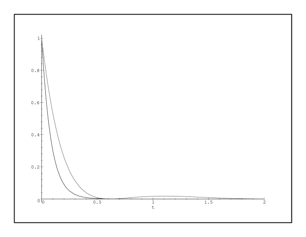
Figure 10: The $t$ - dependence of the ratio $Ra$ for the “black” disc model ( dashed line ) and for the exponential parameterization ( solid line ).

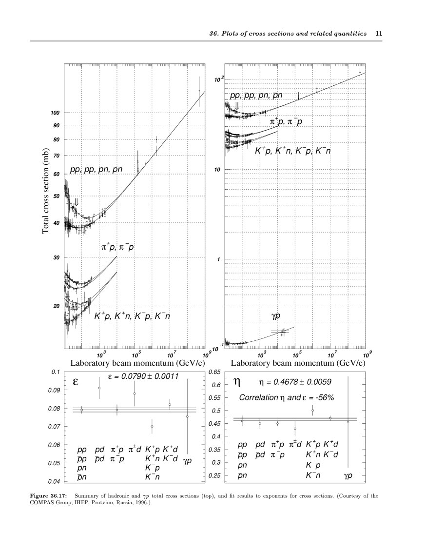
Figure 11-a: The experimental data on the total cross section ( Particle Data Group 1996 ) .

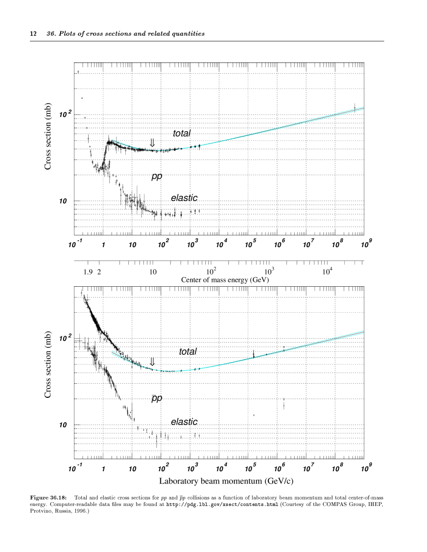
Figure 11-b: The experimental data on total and elastic cross sections ( Particle Data Group 1996 ).

Figure 12: Differential elastic cross section.

3 The first puzzle and Reggeons.

3.1 The first puzzle.

The first puzzle can be formulated as a question:What happens in t- channel exchange of resonances for which the spin is bigger than 1 ?” On the one hand such resonances have been observed experimentally, on the other hand the exchange of the resonances with spin $j$ leads to the scattering amplitudes to be proportional to $s^{j}$ where $s$ is the energy of two colliding hadrons. Such a behaviour contradicts the Froissart bound. It means that we have to find the theoretical solution to this problem.

We have considered the exchange of a vector particle and saw that it gives an amplitude which grows as $s$. Actually, using this example, it is easy to show that the exchange of a resonance with spin $j$ gives rise to a scattering amplitude of the form

$$A^{res}(s,t=-q^{2}_{t})\,=\,g_{1}\,g_{2}\,\frac{(4s)^{j}}{q^{2}_{t}+m^{2}_{R}}\,\,.$$ (38)

Indeed, the amplitude for a resonance in the $t$-channel (for the reaction with energy $\sqrt{t}$ ) is equal to

$$A^{res}(s,t)\,\,=\,\,(2j+1)g_{1}(t)g_{2}(t)\frac{P_{j}(z)}{t-M^{2}_{R}-i\Gamma}\,\,,$$ (39)

As we know $g_{i}$ has an additional kinematic factor $k^{j}$ where $k$ is momentum of decay particles measured in the frame with c.m. energy $\sqrt{t}$. $z$ is the cosine of the scattering angle in the same frame. To find the high energy asymptotic behaviour we need to continue this expression into the scattering kinematic region where $t<0$ and $z\,\rightarrow\,\frac{s}{2k^{2}}\,\gg\,\,1$. This is easy to do, if we notice that $P_{j}(z)\,\rightarrow\,z^{j}$ at $z\,\gg\,1$ and all non- analytical factors ( of $k^{j}$ - type ) cancel in Eq. (39). Recalling that $t\,\rightarrow\,-q^{2}_{t}$ at high energy we obtain Eq. (38), neglecting the width of the resonance in first approximation. In terms of $b$ Eq. (39) looks as follows:

$$A\,\,\propto\,\,s^{j}\,exp(-m_{R}b)$$

at large values of $b$ and $s$.

Of course, the exchange of a single resonance gives a real amplitude and, therefore, does not contribute to the cross section since the total cross section is proportional to the imaginary part of the amlitude accordingly to the optical theorem. To calculate the imaginary part of the scattering amplitude we can use the unitarity constraint, namely

$$ImA(s,t=0)\,\,=\,\,\int\,d^{2}q\delta({p"}^{2}-M^{2}_{1})\delta({p"}^{2}_{2}-M^{2}_{2})\,\,|A^{res}(s,q^{2})|^{2}\,\,.$$ (40)

Recalling that the phase space factor is $d^{4}q\,\,=\,\,\frac{|s|}{2}d\alpha_{q}\beta_{q}d^{2}q_{t}$ where the values of $\beta_{q}$ and $\alpha_{q}$ given in Eq.(30) ( all other notations are clear from Fig.9), we can perform the integration in Eq. (40). It is clear that at high energy

$$ImA(s,t=0)\,\,\propto\,\,s^{2j\,-\,1}\,\,.$$

This equation can be easily generalize for the case of the contribution to the total cross section due to exchange of two particles with spin $j_{1}$ and $j_{2}$, namely

$$\sigma_{tot}\,\,\propto\,\,s^{j_{1}\,+\,j_{2}\,-\,2}\,\,.$$ (41)

This formula is very instructive when we will discuss the contribution of different exchange at high energies. From Eq. (41) it is seen that the exchange of the resonance with spin bigger than 1 leads to a definite violation of the Froissart theorem.

3.2 Reggeons - solutions to the first puzzle.

The solution to the first puzzle is as follows. It turns out that when considering the exchange of a resonance with spin $j$ one has to include also all exitation with spin $j+2$, $j+4$, … (keeping all other quantum numbers the same). These particles lie on a Regge trajectory $\alpha_{R}(t)$ with $\alpha_{R}(t=M^{2}_{j})=j$. The contribution to the scattering amplitude of the exchange of all resonances can be described as an exchange of the new object - Reggeon and its contribution to the scattering amplitude is given by the simple function:

$$A_{R}(s,t)\,\,=\,\,g_{1}(m_{1},M_{1},t)\,g_{2}(m_{2},M_{2},t)\cdot\frac{s^{\alpha(t)}\,\pm\,(-s)^{\alpha(t)}}{sin\pi\alpha(t)}$$ (42)

$\alpha(t)$ is a function of the momentum transfer which we call the Reggeon trajectory.

Figure 13: The Reggeon exchange.

The name of the new object as well as the form of the amplitude came from the analysis of the properties of the scattering amplitude in the $t$ channel using the angular momentum representation. For the following one does not need to follow the full historical development. We need only to understand the main properties of the above function which plays a crucial role in the theory and phenomenology of high energy interactions.

4 The main properties of the Reggeon exchange.

4.1 Analyticity.

First, let me recall that function $(-s)^{\alpha(t)}$ is an analytical function of the complex variable $s$ with the cut starting from $s$ = 0 and going to infinity ( $+\infty$ ) along the $x$ - axis. One can calculate the discontinuaty along this cut. To do this you have to take two values of $s$: $s+i\epsilon$ and $s-i\epsilon$ and calculate

$$\Delta(-s)^{\alpha(t)}\,\,=\,\,2iIm(-s)^{\alpha(t)}\,\,=\,\,s^{\alpha(t)}\,\{e^{i\alpha(t)\pi(1-\frac{\epsilon}{s})}\,\,-\,\,e^{-\,is^{\alpha(t)}\pi(1-\frac{\epsilon}{s}}\,\,=\,\,2isin(\,\pi\,\alpha(t)\,)\,s^{\alpha(t)}\,\,.$$

After these remarks it is obvious that the Reggeon exchange is the analytic function in $s$, which in the $s$ - channel has the imaginary part

$$\pm\,g_{1}\,g_{2}\,s^{\alpha(t)}$$

and in the $u$ - channel the imaginary part

$$g_{1}\,g_{2}\,s^{\alpha(t)}$$

i ( for $\bar{a}+b\rightarrow\bar{a}+b$ reaction ). For different signs in Eq. (42) the function has different properties with respect to crossing symmetry. For plus ( positive signature) the function is symmetric while for minus ( negative signature ) it is antisymmetric.

4.2 s - channel unitarity

To satisfy the $s$ - channel unitarity we have to assume that the trajectory $\alpha(t)\leq 1$ in the scattering kinematic region ( $t<0$ ). In this way the exchange of Reggeons can solve our first puzzle.

4.3 Resonances.

Let us consider the same function but in the resonance kinematic region at $t>M^{2}_{0}$. Here $\alpha(t)$ is a complex function. If $t\rightarrow t_{0}$ then $\alpha(t_{0})\,=\,j\,=\,2k$ ( or $\alpha_{0}(t)\,=\,j\,=\,2\,k+1$,it depends on the sign in Eq.(42)) where $k=1,2,3,..$. The Reggeon exchange for positive signature has a form:

$$A_{R}(s,t)\,\,\rightarrow_{t\rightarrow t_{0}}g_{1}\,g_{2}\cdot\frac{s^{2k}}{\alpha^{\prime}(t_{0})\,(t-t_{0})\,-\,iIm\alpha(t_{0})}$$ (43)

Since in this kinematic region the amplitude $A_{R}$ describes the reaction $\bar{a}+a\rightarrow\bar{b}+b$

$$s\,\,=\,\,p^{2}sin\theta$$

where $p\,=\,\frac{\sqrt{t_{0}}}{2}$, the amplitude has the form

$$A_{R}\,\,=\,\,g_{1}\,g_{2}\cdot\frac{s^{j}}{\alpha^{\prime}(t_{0})(t-t_{0})\,-\,iIm\alpha(t_{0})}\,\,=\,\,\frac{g_{1}g_{2}}{\alpha^{\prime}(t_{0})}\cdot\frac{p^{2j}sin^{j}\theta}{t-t_{0}-i\Gamma}$$ (44)

where the resonance width $\Gamma=\frac{Im\alpha(t_{0})}{\alpha^{\prime}(t_{0})}$.

Therefore the Reggeon gives the Breit - Wigner amplitude of the resonance contribution at $t>4M^{2}_{0}$. It is easy to show that the Reggeon exchange with the negative signature describes the contribution of a resonance with odd spin $j=2k+1$.

4.4 Trajectories.

We can rephrase the previous observation in different words saying that a Reggeon describes the family of resonances that lies on the same trajectory $\alpha(t)$. It gives us a new approach to classification of the resonances, which is quite different from usual $SU_{3}$ classification.

Figure 14: The experimental $\rho$, $f$ and $a$ trajectories .

Fig.14 shows the bosonic resonances classified by Reggeon trajectories. The surprising experimental fact is that all trajectories seem to be approximately straight lines

$$\alpha(t)\,\,=\,\,\alpha(0)\,\,+\,\,\alpha^{\prime}\,t$$ (45)

with the similar slope $\alpha^{\prime}\simeq 1GeV^{-2}$.

We would like to draw your attention to the fact that this simple linear form comes from two experimental facts: 1) the width of resonances are much smaller than their mass ($\Gamma_{i}\,\ll\,M_{R_{i}}$) and 2) the slope of the trajectories which is responsible for the shrinkage of the diffraction peak turns out to be the same from the experiments in the scattering kinematic region.

$SU_{3}$ symmetry requires that

$$\alpha_{\rho}(0)\,=\,\alpha_{\omega}(0)\,=\,\alpha_{\phi}(0)$$

and the slopes to have the same value. The simple picture drawn in Fig.14 shows the intercept $\alpha(0)\,\simeq 0.5$. Therefore the exchange of Reggeons leads to the cross section which falls as a function of the energy and therefore do not violate the Froissart theorem.

4.5 Definite phase.

The Reggeon amplitude of Eq. (42) can be rewritten in the form:

$$A_{R}\,\,=\,\,g_{1}g_{2}\eta_{\pm}s^{\alpha(t)}$$ (46)

where $\eta$ is the signature factor

$$\eta_{+}\,\,=\,\,ctg\frac{\pi\alpha(t)}{2}\,\,+\,\,i$$

$$\eta_{-}\,\,=\,\,tg\frac{\pi\alpha(t)}{2}\,\,-\,\,i\,\,.$$

The exchange of a Reggeon defines also the phase of the scattering amplitude. This fact is very important especially for the description of the interaction with a polarized target.

4.6 Factorization.

The amplitude of Eq. (42) has a simple factorized form in which all dependences on the particular properties of colliding hadrons are concentrated in the vertex functions $g_{1}$ and $g_{2}$. To make this clear let us rewrite this factorization property in an explicit way:

$$A_{R}\,\,=\,\,g_{1}(m_{1},M_{1},q^{2}_{t})\,g_{2}(m_{2},M_{2},q^{2}_{t})\cdot\eta_{\pm}\cdot s^{\alpha(q^{2}_{t})}$$ (47)

For example, it means that if we try to describe the total cross section of the deep inelastic scattering of virtual photon on a target through the Reggeon exchange, only the vertex function should depend on the value of the virtuality of photon ($Q^{2}$) while the energy dependence ( or the intercept of the Reggeon ) does not depend on $Q^{2}$.

It should be stressed that these factorization properties are the direct consequences of the Breit - Wigner formula in the resonance kinematic region ( $t\,\geq\,4m^{2}_{\pi}$).

4.7 The Reggeon exchange in $b$.

It is easy to show that Reggeon exchange has the following form in $b$:

$$a_{R}(s,b)\,\,=\,\,g_{1}(0)\,g_{2}(0)s^{\alpha(0)}\cdot\frac{1}{4\pi(R^{2}_{1}+R^{2}_{2}+\alpha^{\prime}\ln s)}\cdot e^{-\,\frac{b^{2}}{4(R^{2}_{1}+R^{2}_{2}+\alpha^{\prime}\ln s)}}$$ (48)

if we assume the simple exponential parameterization for the vertices:

$$g_{1}(q^{2}_{t})=g_{1}(0)\,e^{-R^{2}_{1}\,q^{2}_{t}}\,\,;$$

$$g_{2}(q^{2}_{t})=g_{2}(0)\,e^{-R^{2}_{2}\,q^{2}_{t}}\,\,.$$

To do this we need to consider the following integral ( see eq.(21) ):

$$a_{R}(s,b)\,\,=\,\,g_{1}(0)\,g_{2}(0)s^{\alpha(0)}\,\frac{1}{2}\int dq^{2}_{t}J_{0}(q_{t}b)\,\,e^{-[\,R^{2}_{1}\,+\,R^{2}_{2}\,+\,\alpha^{\prime}\,\ln s\,]\,q^{2}_{t}}\,\,,$$

which leads to Eq. (48). From Eq. (48) one can see that Reggeon exchange leads to a radius of interaction, which is proportional to $\sqrt{R^{2}_{1}\,+\,R^{2}_{2}\,+\,\alpha^{\prime}\,\ln s}\,\,\rightarrow\,\,\sqrt{\alpha^{\prime}\ln s}$ at very high energy. We recall that in the “black disc ” ( Froissart ) limit the radius of interaction increases proportional to $\ln s$ only. Therefore, we see that Reggeon exchange gives a picture which is quite different from the “ black disk” one.

4.8 Shrinkage of the diffraction peak.

Using the linear trajectory for Reggeons it is easy to see that the elastic cross section due to the exchange of a Reggeon can be written in the form:

$$\frac{d\sigma_{el}}{dt}\,\,=\,\,g^{2}_{1}(q^{2}_{t})\cdot g^{2}_{2}(q^{2}_{t})\cdot s^{2(\alpha(0)-1)}\cdot e^{-2\alpha^{\prime}(0)\,\ln s\,q^{2}_{t}}$$ (49)

The last exponent reflects the phenomena which is known as the shrinkage of the diffraction peak. Indeed, at very high energy the elastic cross section is concentrated at values of $q^{2}_{t}<\frac{1}{\alpha^{\prime}\ln s}$. It means that the diffraction peak becomes narrower at higher energies.

5 Analyticity + Reggeons.

5.1 Duality and Veneziano model.

Now we can come back to the main idea of the approach and try to construct the amplitude from the analytic properties and the Reggeon asymptotic behaviour at high energy. Veneziano suggested the scattering amplitude is the sum of all resonance contributions in $s$ - channel with zero width and, simultaneously, the same amplitude is the sum of the $t$ - channel exchanges of all possible Reggeons.

Figure 15: Duality between the resonances in the $s$-channel and Reggeon exchange in the $t$- channel.

Taking a simplest case the scattering of a scalar particle, the Veneziano amplitude looks as follows:

$$A\,\,=\,\,g\,[\,V(s,t)\,+\,V(u,t)\,+\,V(s,u)\,]$$ (50)

where

$$V(s,t)\,\,=\,\,\frac{\Gamma(1-\alpha(t))\Gamma(1-\alpha(s))}{\Gamma(1-\alpha(t)-\alpha(s))}$$ (51)

$\Gamma(z)$ is the Euler gamma function defined as $\Gamma(z)\,=\,\int^{\infty}{0}\,e^{-t}\,t^{z-1}\,dt$ for $Rez\,>\,0$. What we need to know about this function is the following:

1.$\Gamma(z)$ is the analytical function of $z$ with the simple poles in $z\,=\,-n\,(n=0,1,2..)$;

2. At $z\,\rightarrow\,-n$ $\Gamma(z)\,\rightarrow\,\frac{(-1)^{n}}{(z+n)n!}$;

3.$\Gamma(z+1)\,\,=\,\,z\,\Gamma(z)$, $\Gamma(1)=1$;

4. At large $z$ $\Gamma(z)\,\rightarrow\,z^{z-\frac{1}{2}}\,e^{-z}\,\sqrt{2\pi}(\,1\,+\,O(\frac{1}{z})\,)$;

5. $lim|_{|z|\rightarrow\infty}\frac{\Gamma(z+a)}{\Gamma(z)}\,e^{-a\ln z}\,=\,1$.

Taking these properties in mind one can see that the Veneziano amplitude has resonances at $\alpha(s)=n+1$ where $n=1,2,3...$, since $\Gamma(z)\rightarrow\frac{1}{z+n}$ at $z\rightarrow-n$. At the same time

$$A\,\,\rightarrow_{s\rightarrow\infty}\,\,\Gamma(1-\alpha(t))[(-\alpha(s))^{\alpha(t)}\,\,+\,\,(-\alpha(u))^{\alpha(t)}]$$

which reproduces Reggeon exchange at high energies.

This simple model was the triumph of our general ideas showing us how we can construct the theory using analyticity and asymptotic. The idea was to use the Veneziano model as the first approximation or in other word as a Born term in the theory and to try to build the new theory starting with the new Born Approximation. The coupling constant $g$ is dimensionless and smaller than unity. This fact certainly also encouraged the theoreticians in 70’s to explore this new approach.

5.2 Quark structure of the Reggeons.

In this section, I would like to recall a consequence of the duality approach, described in Fig.15, namely, any Reggeon can be viewed as the exchange of a quark - antiquark pair in the $t$ - channel. Indeed, the whole spectrum of experimentally observed resonances can be described as different kinds of excitation of either a quark - antiquark pair for mesons or of three quarks for baryons. This fact is well known and is one of the main experimental results that led to QCD. In Fig.16 we draw the quark diagrams reflecting the selection rules for meson - meson and meson - baryon scattering. One can notice that all diagrams shown have quark - antiquark exchange in the $t$ - channel. Therefore, the Reggeon - resonance duality leads to the quark - antiquark structure of the Reggeons. I would like to mention that I do not touch here the issue of so called baryonic Reggeons which contribute to meson - baryon scattering at small values of $u$, since our main goal to discuss the Pomeron here, which is responsible for the total cross section or for the scattering amplitude at small $t$.

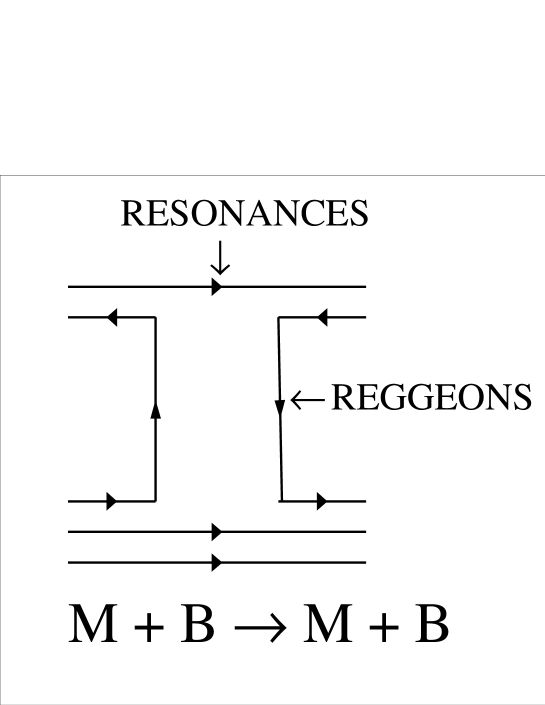
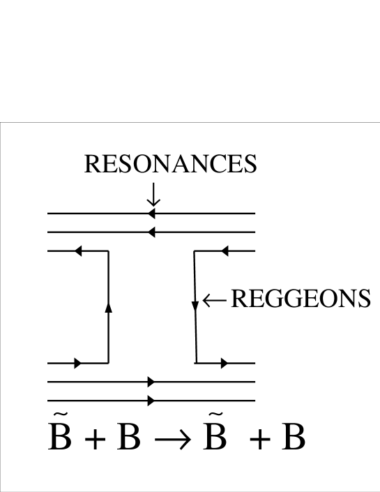
Figure 16: Quark diagrams for meson - meson and meson - baryon scattering.

A clear manifestation of these rules is the fact that reggeons do not contribute to the total cross sections of either proton - proton or to $K^{+}p$ collisions. For both of these processes we cannot draw the diagram with quark - antiquark exchange in the $t$ - channel and /or with three quarks ( quark - antiquark pair) in $s$ - channel (see Fig.17).

Figure 17: Quark diagrams for elastic proton - proton and $K^{+}p$ scattering.

In Reggeon language the quark - antiquark structure of Reggeons leads to so called signature degeneracy. All Reggeons with positive and negative signature have the same trajectory. Actually, this was shown in Fig.14.

Topologically, the duality quark diagrams are planar diagrams. It means that they can be drawn in one sheet of paper without any two lines would be crossed. It is worthwhile mentioning, that all more complicated diagrams, like the exchange of many gluons inside of planar diagrams, lead to the contributions which contain the maximal power of $N_{c}$ where $N_{c}$ is the number of colours. Therefore, in the limit where $\alpha_{\rm S}\,\ll\,1$ but $\alpha_{\rm S}N_{c}\,\approx\,1$ only planar diagrams give the leading contribution.

Figure 18: An example of a planar diagram in the $N_{c}\,>\,1$ approximation.

6 The second and the third puzzles: the Pomeron?!

6.1 Why we need the new Reggeon - the Pomeron?

The experiment shows that:

1. There are no particles ( resonances) on a Reggeon trajectory with an intercept close to unity ( $\alpha(0)\rightarrow 1$). As mentioned before the typical highest has an intercept of $\alpha(0)\sim 0.5$ which generates a cross section $\sigma_{tot}\propto s^{\alpha(0)-1}\propto s^{-\frac{1}{2}}$. Hence, we introduced Reggeons to solve the first puzzle and found to our surprise that these Reggeons give us a total cross section which decreases rapidly at high energy.

2.The measured total cross sections are approximately constant at high energy. We see that fighting against the rise of the cross section due to exchange of high spin resonances got us into the problem to describe the basic experimental fact that the total cross hadron - hadron sections do not decrease with energy.

We call the above two statement the second and the third puzzles that have to be solved by theory. The ad-hoc solution to this problem was the assumption that a Reggeon with the intercept close to 1 exists. One than had to understand how and why this Reggeon is different from other Reggeons, in particular, why there is no particle on this trajectory. Now let us ask ourselves why we introduce one more Reggeon? And we have to answer: only because of the lack of imagination. We can also say that we did not want to multiply the essentials and even find some philosopher to refer to. However, it does not make any difference and one cannot hide the fact that the new Reggeon is just the simplest attempt to understand the constant total cross section at high energy.

As far as I know the first who introduce such a new Reggeon was V.N. Gribov who liked very much this hypothesis since it could explain two facts: the constant cross section and the shrinkage of the diffraction peak in high energy proton - protron collision . By the way, high energy was $s\,\approx\,10-20GeV^{2}$ !!! However, I have to remind you that at that time ( in early sixties ) the popular working model for high energy scattering was the “black disck” approach with the radius which does not depend on energy. Certainly, such a model was much worse than a Reggeon and could not be consistent with our general properties of analyticity and unitarity as was shown by. V.N. Gribov. Of course, on this background the Reggeon hypothesis was a relief since this new Reggeon could exist in a theory. I hope to give you enough illustration of the above statement during the course of the lectures.

Now, let me introduce for the first time the word Pomeron. The first definition of the Pomeron:

The Pomeron is the Reggeon with $\alpha(0)-1\,\equiv\,\Delta\,\ll\,1$

The name Pomeron was introduced in honour of the Russian physicist Pomeranchuk who did a lot to understand this funny object. By the way, the general name of the Reggeon was given after the Italian physicist Regge, who gave a beautiful theoretical argument why such objects can exist in quantum mechanics.

The good news about the Pomeron hypothesis is that it leads to a large number of predictions since the Pomeron should possess all properties of a Reggeon exchange ( see the previous section). And in fact, all Reggeon properties have been established experimentally for the Pomeron.

6.2 Donnachie - Landshoff Pomeron.

The phenomenology, based on the Pomeron hypothesis turned out to be very successful. It survived, at least two decades and even if you do not like the hypothesis you have to learn about it nowdays to cope with the large amount of experimental information on the high energy behaviour of strong interactions.

Let me summarize what we know about the Pomeron from experiment:

1. $\Delta\,\simeq\,0.08$

2. $\alpha^{\prime}(0)\,\simeq\,0.25GeV^{-2}$

Donnachie and Landshoff gave an elegant description of almost all existing experimental data using the hypothesis of the Pomeron with the above parameters of its trajectory. The fit to the data is good. Let us use this DL Pomeron as an example to which we are going to apply everything that we have learned.

The first regretful property of the DL Pomeron is the fact that it violates unitarity since $\Delta\,>\,1$. However, the Froissart limit requires $\sigma_{tot}\,<\,30mb\,N^{2}\ln^{2}s/s_{0}$. Taking $N=1$ and $s_{0}=100GeV^{2}$ we have $\sigma_{tot}\,<\,300\,mb$ for $\sqrt{s}=1800GeV$ ( Tevatron energy ). Therefore, at first sight, the theoretical problem with unitarity exists but we are far away from this problem in all experiments in the near future.

However, we have to be more careful with such statements, since the unitarity constraint is much richer than the Froissart limit. Indeed, from the general unitarity constraint we can derive the so called “weak unitarity”, namely

$$Ima_{el}(s,b)\,\,\leq\,\,1\,\,,$$ (52)

which follows directly from the general solution for the unitarity constraint,

$$Ima_{el}(s,b)\,\,=\,\,1\,\,-\,\,e^{-\frac{\Omega}{2}}\,\,\leq\,\,1\,\,.$$ (53)

For the DL Pomeron we can calculate the amplitude for Pomeron exchange in impact parameter representation ( see Eq. (48) ). The result is

$$a^{DL}_{el}\,\,=\,\,\frac{\sigma(s=s_{0})}{4\,\pi\,[\,2R^{2}_{p}(s=s_{0})\,+\,\alpha^{\prime}\,\ln(s/s_{0})\,]}\,\,(\frac{s}{s_{0}})^{\Delta}\,\,e^{-\,\frac{b^{2}}{4[\,2R^{2}_{p}(s=s_{0})\,+\,\alpha^{\prime}\,\ln(s/s_{0})\,]}}\,\,=$$ (54)

$$\,\,\frac{\sigma(s=s_{0})}{4\,\pi\,B_{el}}\,\,(\frac{s}{s_{0}})^{\Delta}\,\,e^{-\frac{b^{2}}{2B_{el}}}\,\,,$$

where $B_{el}$ is the slope for the elastic cross section ($\frac{d\sigma}{dt}=\frac{d\sigma}{dt}|_{t=0}\,e^{-B_{el}|t|}$). One can see, taking the numbers from Fig.11, that $a^{DL}_{el}(s,b=0)\,\sim\,1/2$ at $\sqrt{s}\,\sim\,100\,GeV$ . For higher energies the DL Pomeron violates the “weak unitarity”.

Therefore, in the range of energies between the fixed target FNAL energies and the Tevatron energy the DL Pomeron cannot be considered as a good approach from the theoretical point of view in spite of the good description of the experimental data. We will discuss this problem later in more details.

I would like to draw your attention to a new parameter $s_{0}$ that has appeared in our estimates ( see Eq.(54) for example). Practically, it enters the master formula of Eq. (47) in the following way

$$A_{R}\,\,=\,\,g_{1}\,g_{2}\,\eta_{\pm}\,\,(\frac{s}{s_{0}})^{\alpha(q^{2}_{t})}\,\,$$

and gives the normalization for the vertices $g_{1}$ and $g_{2}$. As you can see in Veneziano approach ( see Eq.(50) ) $s_{0}\,=\,\frac{1}{\alpha^{\prime}_{R}}\,\approx\,1\,GeV^{2}$. However, in spite of the fact that the value of $s_{0}$ does not affect any physical result since the value of vertices $g_{i}$ we can get only from fitting the experimental data the choice of the value of $s_{0}$ reflect our believe what energy are large. The Reggeon approach is asymptotic one and it can be applied only for large energies $s\,\>\,s_{0}$. Therefore, $s_{0}$ is the energy starting from which we believe that we can use the Reggeon approach.

7 The Pomeron structure in the parton model.

7.1 The Pomeron in the Veneziano model ( Duality approach).

As has been mentioned the Pomeron does not appear in the new Born term of our approach. Therefore, the first idea was to attempt to calculate the next to the Born approximation in the Veneziano model. The basic equation that we want to use is graphically pictured in Fig.19, which is nothing more than the optical theorem.

Figure 19: The Pomeron structure in the duality approach.

We need to know the Born approximation for the amplitude of production of $n$ particles. Our hope was that we would need to know only a general features of this production amplitude to reach an understanding of the Pomeron structure.

To illustrate the main properties and problems which can arise in this approach let us calculate the contribution in equation of Fig. 19 of the first two particle state ( $\sigma^{(2)}_{tot}$). This contribution is equal to:

$$\sigma^{(2)}_{tot}\,\,=\,\,s^{2(\alpha_{R}(0)-1)}\,\,\int d^{2}q^{\prime}_{t}\Gamma^{2}(1-\alpha(-q^{\prime 2}_{t}))\cdot e^{-2\alpha^{\prime}q^{\prime 2}_{t}\ln s}\,\,.$$ (55)

Since

$$\Gamma(1-\alpha(-q^{\prime 2}_{t}))\,\propto\,(-\,\frac{\alpha(-q^{\prime 2}_{t})}{e})^{-\,2\alpha(-q^{\prime 2}_{t})}\,\,\rightarrow\,\,e^{\alpha^{\prime}q^{2}_{t}\ln(\alpha^{\prime}q^{2}_{t})}$$

one can see that the essential value of $q^{\prime}$ in the integral is rather big, namely of the order of $q^{\prime 2}_{t}\,\sim s$. This means that we have to believe in the Veneziano amplitude at larges values of the momentum transfer. Of course nobody believed in the Veneziano model as the correct theory at small distances neither 25 years ago nor now. However we have learned a lesson from this exercise ( the lesson!),namely

To understand the Pomeron structure we have to understand better the structure of the scattering amplitude at large values of the momentum transfer or in other words we must know the interaction at small distances.

7.2 The topological structure of the Pomeron
in the duality approach.

The topological structure of the quark diagrams for the Pomeron is more complicated. Actually, it corresponds to the two sheet configuration . It means that we can draw the Pomeron duality diagram, without any two lines being crossed, not in the sheet of paper but on the surface of a cylinder. For us even more important is that the counting the power of $N_{c}$ shows that the Pomeron leads to one power of $N_{c}$ less than the planar diagram. In Fig.19 you can see the reduction of the duality quark diagram to QCD gluon exchange (gluon “ladder” diagram). Counting of the $N_{c}$ factors shows that the amplitude for emission of $n$-gluon is $\propto\,\,\alpha_{\rm S}^{2+n}\,N^{1+n}_{c}$. Therefore, the approach becomes a bit messy. Strictly speaking there is no Pomeron in leading order of $N_{c}$, but in spite of the fact that it appears in the next order with respect to $N_{c}$ the $s$-dependence can be so strong that it will compensate this smallness. The estimate for ratio yields:

$$\frac{Pomeron}{Reggeon}\,\,\propto\,\,\frac{\alpha_{\rm S}}{N_{c}}(\frac{s}{s_{0}})^{\Delta-\alpha_{R}(0)+1}\,\,\approx\,\,\frac{\alpha_{\rm S}}{N_{c}}(\frac{s}{s_{0}})^{0.51}\,\,.$$

7.3 The general origin of $\ln^{n}s$ contributions.

We show here that the $\ln^{n}s$ contribution results from phase space and, because of this, such logs appear in any theory (at least in all theories that I know). The main contribution to equation of Fig.19 comes from a specific region of integration. Indeed, the total cross section can be written as follows:

$$\sigma_{tot}\,\,=\,\,\Sigma_{n}\int|M^{2}_{n}(x_{i}p,k_{ti})|\Pi_{i}\frac{dx_{i}}{x_{i}}\,\,d^{2}k_{ti}$$ (56)

where $x_{i}$ is the fraction of energy that is carried by the $i$-th particle. Let’s call all secondary particle partons. One finds that the biggest contribution in the above equation comes from the region of integration with strong ordering in $x_{i}$ for all produced partons,namely

$$x_{1}\,\gg\,x_{2}\,\gg.....\gg\,x_{i}\,\gg\,\,x_{i+1}\,\gg.....\gg\,x_{n}\,=\,\frac{m^{2}}{s}$$ (57)

Integration over this kinematic region allows to put all $x_{i}=0$ into the amplitude $M_{n}$. Finally,

$$\sigma_{tot}\,\,=\,\,\Sigma_{n}\int\Pi_{i}d^{2}k_{ti}|M^{2}_{n}(k_{ti})|\,\int^{1}_{\frac{m^{2}}{s}}\,\frac{dx_{1}}{x_{1}}.....\int^{x_{i-1}}_{\frac{m^{2}}{s}}\,\frac{dx_{i}}{x_{i}}\,...\int^{x_{n-1}}_{\frac{m^{2}}{s}}\,\frac{dx_{n}}{x_{n}}$$ (58)

$$=\,\,\Sigma_{n}\int\Pi_{i}d^{2}k_{ti}|M^{2}_{n}(k_{ti})|\,\cdot\,\frac{1}{n!}\,\ln^{n}s$$

This equation shows one very general property of high energy interactions, namely the longitudinal coordinates ( $x_{i}$) and the transverse ones ($k_{ti}$) are separated and should be treated differently. The integration over longitudinal coordinates gives the $\ln^{n}s$ - term. It does not depend on a specific theory , while the transverse momenta integration depends on the theory and is a rather complicated problem to be solved in general. In some sense the above equation reduced the problem of the high energy behaviour of the total cross section to the calculation of the amplitude $M_{n}$ which depends only on transverse coordinates. Assuming, for example, that $\int\Pi d^{2}k_{ti}|M^{2}_{n}(k_{ti})|^{2}\,\propto\frac{1}{m^{2}}g^{n}$ we can derive from the eq.(58)

$$\sigma_{tot}\,=\,\frac{1}{m^{2}}\,\Sigma_{n}\,\frac{g^{n}}{n!}\,\ln^{n}s\,=\,\frac{1}{m^{2}}\cdot s^{g}$$ (59)

which looks just as Pomeron - like behaviour. This example shows the way how the Pomeron can be derived in the theory.

Let us consider a more sophisticated example, the so called $g\phi^{3}$ - theory. This theory has a nice property, namely, the coupling constant is dimension and all integrals over transverse momenta are convergent. Such a theory is one of the theoretical realizations of the Feynman - Gribov parton model, in which was assumed that the mean transverse momentum of the secondary particles ( partons) does not depend on the energy ($k_{it}\,=\,Const(s)$). The parton model is the simplest model for the scattering amplitude at small distances which reproduces the main experimental result in deep inelastic scattering. For us it seems natural to try this model for the structure of the Pomeron. To do this, let us first formulate the approximation in which we are going to work: the leading log$s$ approximation (LLA). In the LLA we sum in each order of perturbation theory, say $g^{n}$, only contributions of the order $(g\ln s)^{n}$, which are big at high energies. As we have discussed the $\ln s^{n}$ term comes from the phase space integration at high energy. To have a contribution of order $(g\ln s)^{n}$ we have to consider a so called ladder diagram (see Fig.20). These ladder diagrams give a sufficiently simple two dimensional theory for $M_{n}(k_{it})$, namely the product of bubble as shown in Fig.20.

Figure 20: The Pomeron in the LLA for $g\phi^{3}$ - theory

One can see that the cross section of emission for the $n$-partons is equal to :

$$\sigma^{n}\,\,=\,\,\frac{1}{s}\frac{\ln^{n}(s/\mu^{2})}{n!}\,\alpha\,\Sigma(q^{2})\,\,(\Sigma(q^{2}))^{n}\,\,$$ (60)

where $\alpha=\frac{g^{2}}{4\pi}$ and

$$\Sigma(q^{2})\,\,=\,\,\alpha\,\,\int\,\frac{d^{2}k_{t}}{(2\pi)^{2}}\,\frac{1}{(\,k^{2}_{t}\,\,+\,\,\mu^{2}\,)\,((k-q)^{2}_{t}\,\,+\,\,\mu^{2}\,)}$$

with $\mu$ being the mass of a parton.

For the total cross section we have:

$$\sigma_{tot}\,\,=\,\,\sum^{\infty}_{n=0}\,\sigma^{n}\,\,=\,\,\frac{1}{s}\,\alpha\,\Sigma(q^{2})(\frac{s}{\mu^{2}})^{\Sigma(q^{2})}\,\,.$$ (61)

Therefore, one can see that we reproduce the Reggeon in this theory with trajectory $\Sigma(q^{2})$. To justify that this Reggeon is a Pomeron we have to show that the intercept of this Reggeon is equal to $1+\Delta$ ( $\Sigma(0)=1+\Delta$ ) as we have discussed. In the LLA of $g\phi^{3}$ - theory we can fix the value of the coupling constant $g$ ( $\alpha$), namely, $\Sigma(0)\,=\,\frac{\alpha}{4\pi\mu^{2}}\,=\,1\,+\,\Delta$ or $\alpha\,=\,(1+\Delta)4\,\pi\,\mu^{2}$. It gives you the parameter of the perturbation approach in $g\phi^{3}$ - theory, $\frac{\alpha}{2\pi\mu^{2}}\,\approx 2$. This sufficiently large value indicates that the LLA can be used onlt as a qualitative attempt to understand the physics of the high energy scattering in this theory but not for serious quantative estimates. Actually, this is the main reason why we are doing all calculation in the LLA of $g\phi^{3}$ - theory but after that we call them parton model approach, expressing our belief that such calculations performing beyond the LLA will reproduce the main qualitative features of the LLA.

7.4 Random walk in $b$.

The simple parton picture reproduces also the shrinkage of the diffraction peak. Indeed, due to the uncertainty principle

$$\Delta b_{i}\,\,k_{ti}\,\sim\,1$$ (62)

or in a different form

$$\Delta b_{i}\,\sim\frac{1}{<k_{t}>}$$

Therefore, after each emission the position of the parton will be shifted by an amount $\Delta b$ which is the same on average.

Figure 21-a: Parton random walk in the transverse plane.

After $n$ emissions we have the picture given in Fig.21a, namely the total shift in $b$ is equal to

$$b^{2}_{n}\,\,=\,\,\frac{1}{<k_{t}>^{2}}\cdot n$$ (63)

which is the typical answer for a random walk in two dimensions ( see Fig.21a). The value of the average number of emissions $n$ can be estimated from the expression for the total cross section (see Eqs.(60)- (61)), since

$$\sigma_{tot}\,=\,\frac{\alpha\Sigma(0)}{s}\,\Sigma_{n}\,\frac{\Sigma^{n}(0)}{n!}\,\ln^{n}\frac{s}{\mu^{2}}\,=\,\sigma_{0}\,\Sigma_{n}\frac{<n>^{n}}{n!}$$

which leads to $<n>\simeq\Sigma(0)\ln s$. If we substitute this value for $<n>$ in the eq.(63 ) we get the radius of interaction

$$R^{2}\,\,=\,\,<b^{2}_{n}>\,\,=\,\,\frac{\Sigma(0)}{<k_{t}>^{2}}\cdot\ln s\,\,.$$

Taking into account the $b$ - profile for the Reggeon ( Pomeron) exchange ( see Eq.( 48 ) ) one can calculate the mean radius of interaction, namely

$$R^{2}\,\,=\,\,\frac{\int d^{2}b\,b^{2}\,\,Im\,a_{R}(s,b)}{\int\,d^{2}b\,Im\,a(s,b)}\,\,=4\,\alpha^{\prime}\,\ln s\,\,.$$

Comparing these two equations we get

$$\alpha^{\prime}\,\,=\,\,\frac{\Sigma(0)}{4\,<k_{t}>^{2}}\,\,.$$

Therefore, in $g\phi^{3}$ theory we obtain the typical properties of Pomeron exchange, but the value of the Pomeron intercept is still an open question which is crucially correlated with the microscopic theory.

In spite of the primitive level of calculations, especially if you compare them with typical QCD calculations in DIS, this model was a good guide for the Pomeron structure for years and, I must admit, it is still the model where we can see everything that we assign to the Pomeron. Therefore, we can formulate the second definition for what the Pomeron is, ( for completeness I repeat the first definition once more):

What is Pomeron?

A1: The Pomeron is the Reggeon with $\alpha_{P}(0)\,-\,1=\,\Delta\,\ll\,\,1$.

A2: The Pomeron is a “ladder” diagram for a superconvergent

theory like $\mathbf{g}\phi^{3}$.

The second definition turns out to be extremely useful for practical purposes, namely, for development of the Pomeron phenomenology, describing a variety of different processes at high energy. This subject will be discussed in the next section. However, let us first describe the very simple picture of the Pomeron structure that results from the second definition.

7.5 Feynman gas approach to multiparticle production.

7.5.1 Rapidity distribution.

Eq. (58) can be rewritten in the new variables transverse momenta and rapidities ofthe produced particles. Let us start from the definition of rapidity ($y$). For particle with energy $E$ and transverse momentum $k_{t}$ the rapidity $y$ is equal to :

$$y\,\,=\,\,\frac{1}{2}\,\ln\frac{E\,+\,p_{L}}{E\,-\,p_{L}}\,\,\rightarrow\,|_{E\,\gg\,max(k_{t},m)}\,\,\ln\frac{2\,E}{m_{t}}\,\,,$$ (64)

where $m^{2}_{t}\,=\,m^{2}\,+\,k^{2}_{t}$.

It is easy to see that the phase space factor in Eq. (58) can be written in terms of rapidities in the following way:

$$\sigma_{tot}\,\,=\,\,\sum_{n}\,\,\int\prod_{i}d^{2}k_{ti}dy_{i}\,|M^{2}_{n}(k_{ti}|\,\,,$$ (65)

with strong ordering in rapidities:

$$y_{1}\,>\,y_{2}\,>\,...\,>\,y_{n-1}\,>\,y_{n}\,\,.$$

This means that Eq. (61) can be interpreted as the sum over the partial cross sections $\sigma^{n}$, each of them is the cross section for the production of $n$ particles uniformly distributed in rapidity ( see Fig.21b).

Figure 21-b: Uniform rapidity distribution of the produced particles in the parton model

7.5.2 Multiplicity distribution.

Eq. (61) can be rewritten in the form:

$$\sigma_{tot}\,\,=\,\,\sigma_{0}\,\sum_{n}\,\sigma^{n}\,\,=\,\,\sigma_{0}\,\sum_{n}\,\frac{<n>^{n}}{n!}\,\,=\,\,\sigma_{0}\,e^{<n>}\,\,,$$ (66)

where $<n>$ is the average multiplicity of the produced partons ( hadrons).

From Eq. (66) one can calculate

$$\frac{\sigma^{n}}{\sigma_{tot}}\,\,=\,\,\frac{<n>^{n}}{n!}\,e^{-<n>}\,\,.$$

This is nothing more than the Poisson distribution. The physical meaning of this distribution is that the produced particles can be considered as a system of free particles without any correlation between them.

7.5.3 Feynman gas.

It is clear ( from Fig.20, for example) that the transverse momentum distribution of one produced particle does not depend how many other particles have been produced. Now, we can collect everything that has been discussed about particle production in the parton model and draw the simple picture for the Pomeron structure:

The Pomeron exchange has the following simple structure:

1. The dominant contribution comes from the production of a large number of particle, namely $\left\langle n\right\rangle\,\,{\mathbf{\propto}\,\,\ln(s/\mu^{2})}$;

2. The produced particles are uniformly distributed in rapidity;

3. The correlations between the produced particles are small and can be neglected in first approximation, therefore, the final state for Pomeron exchange can be viewed as the perfect gas ( Feynman gas ) of partons ( hadrons) in the cylinderical phase space with the coordinates: rapidity $y$ and transverse momentum ($k_{t}$) ( see Fig.21c).

This simple picture generalizes our experience with the parton model and with the experimental data. I am certain that this picture is our reference point in all our discussions of the Pomeron structure. I think that the real Pomeron is much more complex but everybody should know these approximations since only this simple picture leads to the Reggeon with such specific properties as factorization, shrinkage of the diffraction peak and so on.

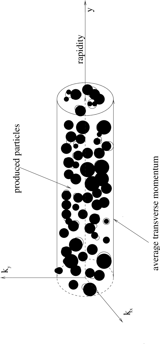
Figure 21-c: The cylinderical phase space for the Feynman gas approximation.

8 Space - time picture of interactions in the parton model.

8.1 Collision in the space - time representation.

To understand the space - time picture of the collision process in the parton model is instructive to rewrite Eq. (58) in the mixed representation,namely, in the variables: transverse momentum $k_{t}$ and two space - time coordinates $x_{+}\,=\,ct\,+\,z$ and $x_{-}\,=\,ct\,-\,z$, where $z$ is the beam direction, for each parton $``i"$. Since the amplitude $M_{n}(k_{ti})$ does not depend on energy and longitudinal momentum, it is easy to write Eq. (58) in such a representation. Indeed, the time - space structure of the $n$ - th term in Eq. (58) reduces to the simple integral ( see Fig.21d for all notations):

$$\int\prod_{i}dt_{i}dz_{i}dt^{\prime}_{i}dz^{\prime}_{i}\int^{E}_{\mu}\,\frac{dE_{1}}{E_{1}}\,e^{i(\,E_{1}(t_{1}\,+\,t^{\prime}_{1})\,\,-\,\,p_{L1}(z_{1}\,+\,z^{\prime}_{1})\,)}...$$ (67)

$$\int^{E_{i-1}}_{\mu}\,\frac{dE_{i}}{E_{i}}\,e^{i(\,E_{i}(t_{i}\,+\,t^{\prime}_{i})\,\,-\,\,p_{Li}(z_{i}\,+\,z^{\prime}_{i})\,)}...$$

$$\int^{E_{n-1}}_{\mu}\,\frac{dE_{n}}{E_{n}}\,e^{i(\,E_{n}(t_{n}\,+\,t^{\prime}_{n})\,\,-\,\,p_{Ln}(z_{n}\,+\,z^{\prime}_{n})\,)}\,\,.$$

Figure 21-d: Space - time picture for high energy interactions in the parton model.

For a high energy parton ($E_{i}\,\gg\,\mu$ ) the longitudinal momentum $p_{Li}\,=\,E_{i}\,-\,\frac{m^{2}{ti}}{2E_{i}}$, where $m^{2}_{ti}\,=\,\mu^{2}\,+\,k^{2}_{ti}$. Therefore,

$$E_{i}(t_{i}\,+\,t^{\prime}_{i})\,\,-\,\,p_{Li}(z_{i}\,+\,z^{\prime}_{i})\,\,=\,\,p_{+,i}\,(\,x_{-,i}\,-\,x^{\prime}_{-,i}\,)\,\,-\,\,p_{-,i}\,(\,x_{+,i}\,-\,x^{\prime}_{+,i}\,)\,\,,$$

where $p_{+,i}\,=\,\frac{E_{i}\,+\,p_{Li}}{2}$ and $p_{-,i}\,=\,\frac{E_{i}\,-\,p_{Li}}{2}$.

For fast partons we have

$$E_{i}(t_{i}\,+\,t^{\prime}_{i})\,\,-\,\,p_{Li}(z_{i}\,+\,z^{\prime}_{i})\,\,\rightarrow\,\,E_{i}\,(c(t_{i}\,+\,t^{\prime}_{i})\,-\,(z_{i}+z^{\prime}_{i}))\,-\,\frac{m^{2}{ti}}{4E_{i}}\,(c(t_{i}\,+\,t^{\prime}_{i})\,+\,(z_{i}+z^{\prime}_{i}))\,\,.$$

Therefore, $c(t_{i}\,+\,t^{\prime}_{i})\,=\,(z_{i}+z^{\prime}_{i})\,+\,O(1/E_{i})$ at high energy. One can also see that the integrand in Eq. (67) does not depend on the variables $t_{i}-t^{\prime}_{i}$ and $z_{i}-z^{\prime}_{i}$. Since the amplitude does not depend on energy and longitudinal momenta, it contains $\delta$ - functions with respect each of these variables. Integrating these two $\delta$ - functions yeilds $t_{i}=t^{\prime}_{i}$ and $z_{i}=z^{\prime}_{i}$. After taking the integral over $c(t_{i}\,+\,t^{\prime}_{i})\,-\,(z_{i}+z^{\prime}_{i})\,$, which leads to an extra power of $E_{i}$ in the dominator, we are left with the following integrations:

$$\int dz_{1}\int^{E}_{\mu}\,\frac{dE_{1}}{E^{2}_{1}}\,e^{-\frac{m^{2}_{t1}}{E_{1}}\,z_{1}}...\int dz_{i}\,\int^{E_{i-1}}_{\mu}\,\frac{dE_{i}}{E^{2}_{i}}\,e^{-\frac{m^{2}_{ti}}{E_{i}}\,z_{i}}\,...\int\,dz_{n}\,\int^{E_{n-1}}_{\mu}\,\frac{dE_{n}}{E^{2}_{n}}\,e^{-\frac{m^{2}_{tn}}{E_{n}}\,z_{n}}\,\,.$$ (68)

Due to the factor $E^{2}_{i}$ in the dominator the main contribution in the integral over $E_{i}$ comes from the region of small $E_{i}$ but $E_{i}\,>\,\frac{z_{i}}{m^{2}_{ti}}$ since the integral is suppressed for smaller energies due to oscillations of the exponent.

Finally, Eq. (58) in space - time coordinates can be written in a form which is very similar to the form of Eq. (58),

$$\sigma_{tot}\,\,=\,\,\Sigma_{n}\int\Pi_{i}d^{2}k_{ti}|{\tilde{M}}^{2}_{n}(k_{ti})|\,\int^{\frac{s}{m^{3}_{t1}}}_{\frac{1}{\mu}}\,\frac{dz_{1}}{z_{1}}.....\int^{z_{i-1}}_{\frac{1}{\mu}}\,\frac{dz_{i}}{z_{i}}\,...\int^{z_{n-1}}_{\frac{1}{\mu}}\,\frac{dz_{n}}{z_{n}}$$ (69)

$$=\,\,\Sigma_{n}\int\Pi_{i}d^{2}k_{ti}|{\tilde{M}}^{2}_{n}(k_{ti})|\,\cdot\,\frac{1}{n!}\,\ln^{n}s\,\,.$$

Fig. 21d illustrates the high energy interactions accordingly to Eq. (69) in the lab. frame, where the target is at the rest. A long time ( $t_{1}\,\propto\,\frac{s}{2mm^{2}_{t1}}$, where $m$ is the target mass while $m^{2}_{t1}$ is the transverse mass of the first parton) before the collision with the target the fast hadron decays into a system of partons which to first approximation can be considered as non - interacting ones. The target interacts only with those partons which have energy and /or longitudinal momentum of the order of the target size, which is $\approx\,1/\mu$. It takes a short time ( of the order of $\frac{1}{\mu}$ ) in comparison with the long time of the whole parton cascade which is of the order of $E/\mu^{2}$ where $E$ is the energy of the incoming hadron. In the parton model we neglect the time of interaction (see Fig.21d) in comparison with the time of the whole parton fluctuation. Therefore, we can rewrite Eq. (69) in the general form:

$$\sigma\,\,=\,\,\sum_{n}|\Psi^{partons}_{n}(t)|^{2}\,\sigma(\,parton\,\,+\,\,target\,)(t)\,\,,$$ (70)

where $\Psi^{partons}_{n}(t)$ is the partonic wave function ( wave function of $n$ - partons) at the moment of interaction $t$ ( $t$ = 0 in Fig.21d ). From Eq. (70) one can see that the target affects only a small number of partons with sufficiently low energies while most properties of the high energy interaction are absorbed into the partonic wave function which is the same for any target. One can recognize the factorization properties of the Pomeron in this picture.

8.2 Probabilistic interpretation.

One can see from Eq. (70) that the physical observable ( cross section ) can be written as sum of $|\Psi_{n}|^{2}$. $|\Psi_{n}|^{2}$ has obviously a physical meaning: it is the probability to find $n$ partons in the parton cascade ( in the fast hadron). Therefore, when discussing the Pomeron structure in the parton model one can forget interference diagrams and all other specific features of quantum mechanics. In some sense we can develop a Monte Carlo simulation for the Pomeron content. This is so because the Pomeron is mostly an inelastic object and one can neglect the contribution of the elastic amplitude to the unitarity constraint.

Figure 21-e: Four stages of high energy interactions in the parton model.

The second important observation is that for each term in the sum of Eq. (70), the transverse and longitudinal degrees of freedom are completely separated and can be treated independently namely a simple uniform distribution in rapidity and a rather complicated field theory for the transverse degrees of freedom.

8.3 “Wee” partons and hadronization.

Taking this simple probabilistic ( parton ) interpretation we are able to explain all features of high energy interactions without explicit calculations. As we have mentioned only very slow parton can interact with the target in the lab. frame. Such active partons are called “wee” partons ( Feynman 1969 ).

Figure 21-f: “Wee” partons and hadrons.

Therefore, in the parton model a high energy interaction proceeds four clearly separated stages (see Fig.21e):

Stage I : Time ($t\,\propto\,\frac{E}{\mu^{2}}$) before interaction of the “wee” parton with the target. The fast hadron can be considered as a state of many point-like particles ( partons) in a coherent state which we describe by the means of a wave function.

Stage II : Short time of interaction of the “wee” parton with the target. The cross section of this interaction depends on the target. The most important effect of the interaction is it destroys the coherence of the partonic wave function.

Stage III : Free partons in the final state which, to first approximation, can be described as Feynman gas.

Stage IV : Hadronization or in other words the creation of the observed hadrons from free partons. There is the wide spread but false belief that the simple parton model has no hadronization stage . We will show in a short while that this is just wrong.

The total cross section of the interaction is equal to

$$\sigma_{tot}(s)\,\,=\,\,N(``wee"\,\,partons)\,\sigma(\,``wee"parton\,+\,target\,)\,\,.$$ (71)

Actually, we can write Eq. (71) in a more detailed form by including the integration over the rapidity of the “wee” parton, namely:

$$\sigma_{tot}(s)\,\,=\,\,\int dy_{wee}\,N(y_{wee})\sigma(y_{wee})\,\,,$$ (72)

and we assume that the cross section for “wee” parton - target interaction decreases as a function of $y_{wee}$ much faster that $y_{wee}$ - dependence in $N$.

We can estimate the dependence of $N$ on the energy. Indeed, a glance on Fig.21f shows that the number of “wee” partons should be very large because each parton can decay into its own chain of partons. Let us assume that we know the multiplicity of partons in one chain ( let us denote it by $<n>$ ). One can show that $N\,\,\propto\,\,e^{<n>}$. Therefore,

$$\sigma_{tot}\,\,\propto\,\,\sigma_{0}\,e^{<n>}\,\,,$$

where $\sigma_{0}$ stands for the “wee” parton - target interaction cross section.

We have calculated $<n>\,\,\approx\,\,\Sigma(o)\,\ln s$ ( subsection 7.4 where we discussed the random walk in the transverse plane ). Graphically, we show this calculation in Fig.21f.

An obvious question is why the multiplicity in one chain coincides with the multiplicity of produced particles as it follows from our calculation of $<n>$ ( see also Fig. 21f). The difference is in the hadronization stage. Indeed, a “wee” parton interacts with the target. We have $N$ “ wee” partons but only one of them interacts. Of course, since it can be any, the cross section is proportional to the total number of “wee” partons. However, if one of the “wee” partons hits the target all other pass the target without interaction. They gather together and contribute to the renormalization of the mass in our field theory ( see Figs. 21e and 21f). Therefore,in the simple partonic picture the number of produced “hadrons” is the same as the number of partons in one parton chain. Of course, this is an oversimplified picture of hadronization, but it should be stressed that even in the simplest field theory such as $g\phi^{3}$ - theory we have a hadronization stage which reduces the number of partons in the parton cascade from $N\,\propto\,e^{<n>}$ to $<n>$.

8.4 Diffraction Dissociation.

As we have discussed the typical final state in the parton model is an inelastic event with large multiplicity and with uniform distribution of the produced hadrons in rapidity. All events with small multiplicity, such as resulting from diffraction dissociation, can be considered as a correction to the parton model which should be small. Indeed, diffraction dissociation events correspond to such interactions of the “wee” parton with the target which do not destroy the coherence of the partonic wave function for most of partons belonging to it. This process is shown in Fig.21g. In Fig.21g one can see that the interaction of a “wee” parton with the target does not change the wave function for all partons with rapidities $y_{i}\,<\,y_{M}$ but destroys the coherence completely for partons with $y_{i}\,>\,y_{M}$. In the next section we show how to describe such processes.

Figure 21-g: Diffractive dissociation in the parton model.

9 Different processes in the Reggeon Approach.

9.1 Mueller technique.

Using the second definition of the Pomeron, namely:“ The Pomeron is a “ladder” diagram for a superconvergent theory like $g\phi^{3}$ one”( better: using the second definition as a guide) we can easily understand a very powerful technique suggested by Al Mueller in 1970. The first observation is that the optical theorem in LLA looks very simple as shown in Fig.22. The Mueller technique can be understood in a very simple way: for every process try to draw ladder diagrams and use the optical theorem in the form of Fig.22.

Figure 22: Optical theorem and inclusive production in the LLA for $g\phi^{3}$-theory ( parton model).

Let us illustrate this technique by considering the single inclusive cross section for production of a hadron $c$ with rapidity $y_{c}$ integrated over its transverse momentum (see Fig.22). Summing over hadrons $n_{1}$ and $n_{2}$ with rapidities more or less than $y_{c}$ and using the optical theorem we can rewrite this cross section as a product of two cross sections with rapidities ( energies) $Y-y_{c}$ and $y_{c}$. Using Pomeron exchange for the total cross section and introducing a general vertex $a$ we obtain a Mueller diagram for the single inclusive cross section. In spite of the fact that this technique looks very simple it is a powerful tool to establish a unique description of exclusive and inclusive processes in the Reggeon Approach. Here we want to write down several examples of processes which can be treated on the same footing in the Reggeon approach.

9.2 Total cross section.

In the one Pomeron exchange approximation the total cross section is given by the following expression (see Fig.23a):

$$\sigma_{tot}\,\,=\,\,4\pi g_{1}(0)\,g_{2}(0)(\frac{s}{s_{0}})^{\Delta}\,\,=\,\,\sigma(s=s_{o})(\frac{s}{s_{0}})^{\Delta}$$ (73)

Remember that multi-Pomeron exchange is very essential for describing the total cross section but we postpone this discussion of their contribution to the second part of our lectures.

The energy behaviour of the total cross section in the region of not too high energy depends on the contribution of the secondary Reggeons. It has become customary to consider only one secondary Reggeon. It is certainly not correct and we have to be careful. For example, for the $p-p$ total cross section we there is a secondary Reggeon with positive signature ($P^{\prime}$ or $f$ Reggeon) and two Reggeons with negative signature ($\omega$ and $\rho$ ). The first one is responsible for the energy dependence of the total cross section and gives the same contribution to $p-p$ and $\bar{p}-p$ collisions. The $\omega$- Reggeon contributes with opposite signs to these two reactions and is responsible for the value and energy dependence of the difference $\sigma_{tot}(\bar{p}p)\,\,-\,\,\sigma_{tot}(pp)\,\propto\,\,(\,\frac{s}{s_{0}}\,)^{\alpha_{\omega}(0)-1}\,\,\approx\,\,(\,\frac{s}{s_{0})}\,)^{-0.5}$.

Finally, the total cross section can be written in the general form

$$\sigma_{tot}\,\,=\,\,4\pi g^{P}_{1}(0)\,g_{2}^{P}(0)\,\,(\frac{s}{s_{0}})^{\Delta}\,\,+\,\,\sum_{R_{i}}(-1)^{S}4\pi g^{R_{i}}_{1}(0)\,g^{R_{i}}_{2}(0)\,\,(\frac{s}{s_{0}})^{\alpha_{R_{i}}(0)-1}\,\,,$$ (74)

where $S=0$ for positive signature and $S=1$ for negative signature Reggeons for particle - particle scattering ( for antiparticle - particle scattering all contributions are positive).

Figure 23-a: Total cross section in the Mueller technique.

9.3 Elastic cross section.

Collecting everything we have learned on Reggeon ( Pomeron ) exchange we can show that for one Pomeron exchange the total elastic cross section is equal to (see Fig.23b )

$$\sigma_{el}\,\,=\,\,\frac{\sigma^{2}_{tot}}{16\pi B_{el}}$$

where

$$B_{el}\,\,=\,\,2R^{2}_{01}\,+\,2R^{2}_{02}\,+\,2\alpha^{\prime}_{P}\ln s/s_{0}$$

in the exponential parameterization of the vertices.

It is interesting to note that this formula is written in the approximation where we neglected the real part of the amplitude. The correct formula is

$$\sigma_{el}\,\,=\,\,\frac{\sigma^{2}_{tot}}{16\pi B_{el}}\,(\,1\,\,+\,\,\rho^{2}\,)\,\,,$$

where $\rho=\frac{ReA(s,t)}{ImA(s,t)}$. For the Pomeron the quantity $\Delta$ is small (see first definition) and

$$\rho\,\,=\,\,\frac{\pi}{2}\,\frac{1}{ImA(s,t)}\,\frac{dImA(s,t)}{d\ln s}\,=\,\frac{\pi}{2}\Delta\,\,.$$

For the secondary trajectories we have to take into account the signature factors ( $\eta_{+}$ or $\eta_{-}$ ) and calculate the real part of the amplitude.

Figure 23-b: Elastic cross section in the Mueller technique.

9.4 Single diffraction dissociation

The cross section for single diffraction (see Fig.23c) has the following form when $M^{2}$ is large):

$$\frac{M^{2}d\sigma_{SD}}{dM^{2}\,dt}\,\,=\,\,\frac{g^{2}_{p}(t)}{4}(\frac{S}{M^{2}})^{2\Delta}\,\sigma_{tot}(2+P)\,\,,$$ (75)

where $\sigma_{tot}$ is the total cross section ofor Pomeron + hadron 2 scattering.

Figure 23-c: Single Diffraction in the Mueller technique.

At first sight, it seems strange that Pomeron exchange depends on the ratio $\frac{s}{M^{2}}$. In LLA for the $g\phi^{2}$ - theory ( parton model ) this process is shown in Fig.23. Here Pomeron exchange certainly depends on the energy $s^{\prime}=x_{i}p_{2}m_{1}$ in the rest frame of hadron 1 ( in lab. frame). In LLA

$$x_{1}\,\gg\,x_{2}\,\gg\,...\gg\,x_{i}$$

and

$$M^{2}\,\,=\,\,(\sum^{i}_{l=1}p_{0l})^{2}-(\sum^{i}_{l=1}p_{Ll})^{2}\,\,\approx\,\,\frac{p^{2}_{it}}{x_{i}}\,\,.$$

Therefore, in the framework of the parton model where $<p^{2}_{t}>$ does not depends on energy,

$$x_{i}\,\,\approx\,\,\frac{<p^{2}_{t}>}{M^{2}}$$

and

$$s^{\prime}\,\,=\,\,2x_{i}p_{2}m_{1}\,\,=\,\,<p^{2}_{t}>\,\cdot\,\frac{s}{M^{2}}\,\,.$$

We absorb some of the factors in the definition of the cross section in Eq. (75).

The next question is how well can we determine the normalization of the Pomeron - hadron cross section. The natural condition for the normalization is that the cross section, defined by Eq. (75), coincides with the cross section of the interaction of hadron 2 with the resonance (R) at $t=m^{2}_{R}$. Of course, when $m_{R}$ is small all formulae give the same answer. However, let us consider the $\rho$ - trajectory and compare the exchange of the $\rho$ - Reggeon at $t=0$ in two different models: the Veneziano model and the simple formula of Eq. (42). Taking $\alpha_{\rho}(t=0)$ = $0.5$ we see that cross section in the Veneziano model is $\pi$ times bigger that in Eq. (42). Therefore, even for Reggeons we have a problem with the normalization. For the Pomeron the situation is even worse since we know there is even one resonance on the Pomeron - trajectory. My personal opinion is that we have to make a common agreement what we will expect for the cross section but we should be very careful in comparison the value of this cross section with that for ordinary hadron - hadron scattering.

In the region where $M^{2}$ is large we can apply for Pomeron - hadron cross section the same expansion with respect to Pomeron + Reggeons exchange ( see Eq. (74)

$$\frac{M^{2}d\sigma_{SD}}{dM^{2}}\,\,=\,\,\frac{\sigma_{0}}{2\pi R^{2}(\frac{s}{M^{2}})}\,\cdot\,(\frac{s}{M^{2}})^{2\Delta}\,\cdot\,[\,G_{3P}(0)\,\cdot\,(\frac{M^{2}}{s_{0}})^{\Delta}\,+\,G_{PPR}(0)(\frac{M^{2}}{s_{0}})^{\alpha_{R}(0)-1}\,]$$ (76)

Let me summarize what we learned experimentally about the triple Pomeron vertex:

1. The value of $G_{3P}$ is smaller than the value of $g_{i}$ ( the hadron - Pomeron vertex): $G_{3P}\,\,\approx 0.1\,g_{i}$;

2. The dependence of the triple Pomeron vertex on $t$ can be characterized by the radius of the triple Pomeron vertex $r_{0}$ ($G_{3P}(t)\,\approx\,e^{-2\,r^{2}_{0}|t|}$), which turns out to be rather small, namely, $r^{2}_{0}\,\leq\,1\,GeV^{-2}$ .

It is easy to show that in the exponential parameterization of the vertices (see Eq. (48))

$$R^{2}(\frac{s}{M^{2}})\,\,=\,\,2R^{2}_{01}\,+\,2r^{2}_{0}\,+\,2\alpha^{\prime}_{P}\ln(s/M^{2})\,\,.$$

9.5 Non-diagonal contributions.

Eq.(76) gives the correct descriptions for the energy and mass behaviour of the SD cross section in the Reggeon phenomenology but only for $\frac{s}{M^{2}}\,\,\gg\,\,1$. For $\frac{s}{M^{2}}\,\approx\,\,1$ we have to modify Eq.(76) by including secondary Reggeons. It means that we have to substitute in Eq.(76)

$$(\,\frac{s}{M^{2}}\,)^{\Delta}\,\,\rightarrow\,\,(\,\frac{s}{M^{2}}\,)^{\Delta}\,\,+\,\,\sum_{i}\,A_{R_{i}}\,(\,\frac{s}{M^{2}}\,)^{\alpha_{R_{i}}(0)-1}\,\,,$$

where $i$ denotes the Reggeon with trajectory $\alpha_{R_{i}}(t)$. As can be seen the $s$ - dependence of Eq. (76) is only governed by the Pomeron ( $M^{2}d\sigma_{SD}/dM^{2}\,\,\propto\,\,s^{2\Delta}$) while Eq. (76-b) leads to a more general energy dependence, namely,

$$\frac{M^{2}d\sigma_{SD}}{dM^{2}}\,\,\propto\,\,\{\,(\,\frac{s}{M^{2}}\,)^{\Delta}\,\,\pm\,\,A_{R}\,(\,\frac{s}{M^{2}}\,)^{\alpha_{R}(0)-1}\,\}^{2}\,\,.$$ (76-a)

Therefore the general equation has the form:

$$\frac{M^{2}d\sigma_{SD}}{dM^{2}\,dt}\,\,=\,\,\sum_{i,j,k}\,\,g_{i}\,g_{j}\,g_{k}\,G_{ijk}\,(\,\frac{s}{M^{2}}\,)^{\Delta_{i}}\,(\,\frac{M^{2}}{s_{0}}\,)^{\Delta_{j}}\,(\,\frac{s}{M^{2}}\,)^{\Delta_{k}}\,\,,$$ (76-b)

where $i$,$j$ and $k$ denote all Reggeons including the Pomeron and $\Delta_{l}\,\,=\,\,\alpha_{l}(0)\,-\,1$ with $l$ = $i$,$j$ and $k$. Note, that factor $(\frac{M^{2}}{s_{0}})^{\Delta_{j}}$ comes from the Pomeron - hadron cross section as has been discussed above ( see Eq. (76) ).

We can see from Eq. (76-b) as well as from Eq. (76-a) that the first correction to the Pomeron induced energy behaviour comes from the so called interference or non-diagonal (N-D) term, which can be written in the general form:

$$\frac{M^{2}d\sigma^{N-D}_{SD}}{dM^{2}\,dt}\,\,=\,\,\sigma_{P+p\rightarrow R+p}(M^{2})\,g_{P}\,g_{R}\,(\,\frac{s}{M^{2}}\,)^{\Delta_{P}}\,(\,\frac{s}{M^{2}}\,)^{\Delta_{R}}\,\,,$$ (76-c)

where $P$ stands for the Pomeron and $R$ for any secondary Reggeon. $\sigma_{P+p\rightarrow R+p}(M^{2})$ can be written as a sum of the Reggeon contributions as

$$\sigma_{P+p\rightarrow R+p}(M^{2})\,\,=\,\,g_{P}\,G_{PPR}\,(\,\frac{M^{2}}{s_{0}}\,)^{\Delta_{P}}\,\,\pm\,\,\,g_{R}\,G_{PPR}\,(\,\frac{M^{2}}{s_{0}}\,)^{\Delta_{R}}\,\,.$$ (76-d)

It is clear that the non-diagonal term gives the first and the most important correction which has to be taken into account in any phenomenological approach to provide a correct determination of the diffractive dissociation contribution. By definition, we call diffractive dissociation only the contribution which survives at high energy or, i.e. it corresponds to the Pomeron exchange term in the Reggeon phenomenology. Unfortunately, we know almost nothing about this non-diagonal term. We cannot guarantee even the sign of the contribution. This lack of our knowledge I have tried to express by putting $\pm$ into the above equations.

Let me discuss here what I mean by “almost nothing”.

First, we can derive an inequality for $\sigma_{P+p\rightarrow R+p}(M^{2})$ using the generalized optical theorem that we discussed in section 9.1. By definition

$$\sigma_{P+p\rightarrow R+p}(M^{2})\,\,=\,\,\frac{1}{2}\sum_{n,q}\{\,g_{P}(M^{2},n,q)\cdot g^{*}_{R}(M^{2},n,q)\,\,+\,\,g_{P}(M^{2},n,q)\cdot g^{*}_{R}(M^{2},n,q)\,\}\,\,,$$

where $n$ is the number of produced particles with mass $M$ and $q$ denotes all other quantum numbers of the final state. Notice that the factor $1/2$ in front is due to the definition in Eq. (76-b) where we sum separately over $PR$ and $RP$ contributions.

The inequality

$$\sum_{n,q}|\,g_{P}(M^{2},n,q)\,-\,z\,g_{R}(M^{2},n,q)\,|^{2}\,\,\geq\,\,0$$

implies for any value of $z$, therefore

$$\sigma^{2}_{P+p\rightarrow R+p}(M^{2})\,\,\leq\,\sigma_{P+p\rightarrow P+p}(M^{2})\cdot\sigma_{R+p\rightarrow R+p}(M^{2})$$ (76-e)

Using Eq. (76-d) and the analogous expressions for the $p+p$ and $R+p$ cross sections, Eq. (76-e) leads to

$$G^{2}_{PPR}\,\,\leq\,\,G_{PPP}\cdot G_{RPR}\,\,;\,\,\,\,\,\,\,\,G^{2}_{PRR}\,\,\leq\,\,G_{PRP}\cdot G_{RRR}\,\,.$$ (76-f)

Actually, Eq. (76-f) is the only reliable knowledge we have on the interference ( non-diagonal ) term. However, in the simple parton model or/and in the LLA of $g\phi^{3}$-theory we know that the sign of the non-diagonal vertices is positive and that the inequality of Eq. (76-f) is saturated:

$$G^{2}_{PPR}\,\,=\,\,G_{PPP}\cdot G_{RPR}\,\,;\,\,\,\,\,\,\,\,G^{2}_{PRR}\,\,=\,\,G_{PRP}\cdot G_{RRR}\,\,.$$ (76-g)

The same result can be obtained in other models where the Pomeron scale is assumed to be larger than the typical hadron size, as for instance, in the additive quark model. However, in general we have no proof for Eq. (76-g) and, therefore, can recommend only to introduce a new parameter $\delta$ and use the following form:

$$G_{PPR}\,\,=\,\,sin\delta_{P}\cdot\sqrt{G_{PPP}\cdot G_{RPR}}\,\,;\,\,\,\,\,\,\,\,G_{PRR}\,\,=\,\,sin\delta_{R}\cdot\sqrt{G_{PRP}\cdot G_{RRR}}\,\,.$$ (76-h)

This section is a good illustration how badly we need a theory for the high energy scattering.

9.6 Double diffraction dissociation.

From Fig.23d one can see that the cross section for double diffraction dissociation ( DD ) process is equal to:

$$\frac{M^{2}_{1}M^{2}_{2}d^{2}\sigma_{DD}}{dM^{2}_{1}dM^{2}_{2}}\,\,=\,\,\frac{\sigma_{0}}{2\pi R^{2}(\frac{ss_{0}}{M^{2}_{1}M^{2}_{2}})}\cdot G^{2}_{3P}(0)\cdot(\frac{ss_{0}}{M^{2}_{1}M^{2}_{2}})^{2\Delta}\cdot(\frac{M^{2}_{1}}{s_{0}})^{\Delta}\cdot(\frac{M^{2}_{2}}{s_{0}})^{\Delta}$$ (77)

in the region of large values of produced masses ( $M_{1}$ and $M_{2}$ ).

It is important to note that the energy dependence is contained in the variable

$$s"\,\,\propto\,\,\frac{ss_{0}}{M^{2}_{1}M^{2}_{2}}\,\,.$$

Repeating the calculation of the previous subsection we see that (see Fig.23d):

$$x^{1}_{i}\,\,=\,\,\frac{<p^{2}_{t}>}{M^{2}_{1}}\,\,;$$ (78)

$$x^{2}_{i^{\prime}}\,\,=\,\,\frac{<p^{2}_{t}>}{M^{2}_{2}}\,\,;$$

and

$$s"\,\,=\,\,2\,x^{1}_{i}\,x^{2}_{i^{\prime}}\,p_{1\mu}\,p_{2\mu}\,\,=\,\,(<p^{2}_{t}>)^{2}\,\,\frac{s}{M^{2}_{1}\,M^{2}_{2}}\,\,\approx\,\,s_{0}\,\frac{s\,s_{0}}{M^{2}_{1}\,M^{2}_{2}}\,\,.$$

Note also, that, in the exponential parameterization of the vertices ( see Eq. (48) ) $R^{2}(\frac{s\,s_{0}}{M^{2}_{1}\,M^{2}_{2}})$ in Eq. (77) is equal to

$$R^{2}(\frac{s\,s_{0}}{M^{2}_{1}\,M^{2}_{2}})\,\,=\,\,2\,r^{2}_{0}\,\,+\,\,2\alpha^{\prime}_{P}\ln(ss_{0}/M^{2}_{1}M^{2}_{2})\,\,.$$

Figure 23-d: Double Diffraction in the Mueller technique.

9.7 Factorization for diffractive processes.

Comparing the cross sections for elastic, double and single diffraction the following factorization relation can be derived:

$$\frac{M^{2}_{1}M^{2}_{2}d^{2}\sigma_{DD}}{dM^{2}_{1}dM^{2}_{2}}\,\,=\,\,\frac{\frac{M^{2}_{1}d\sigma_{SD}}{dM^{2}_{1}}\frac{M^{2}_{2}d\sigma_{SD}}{dM^{2}_{2}}}{\sigma_{el}}\,\cdot\,\frac{R^{2}(\frac{s}{M^{2}_{1}})R^{2}(\frac{s}{M^{2}_{2}})}{R^{2}(\frac{ss_{0}}{M^{2}_{1}M^{2}_{2}})R^{2}_{el}(s)}$$ (79)

where

$$R^{2}_{el}=2R^{2}_{01}+2R^{2}_{02}+2\alpha^{\prime}_{P}\ln(s/s_{0})$$

The event structure for double diffraction is sketched in Fig.24 in a lego - plot. No particles are produced with rapidities $\Delta y=\ln\frac{ss_{0}}{M^{2}_{1}M^{2}_{2}}$.

9.8 Central Diffraction.

This process leads to production of particles in the central rapidity region, while there are no particles in other regions of rapidity.

The cross section for the production of particles of mass $M$ in proton - proton collision can be written in the form:

$$M^{2}\,\frac{d\sigma}{dM^{2}}\,\,=\,\,\sigma_{PP}\,\sigma^{2}_{pp}\,\frac{1}{R^{2}_{0p}\,+\,\alpha^{\prime}_{P}(0)\,\ln(s/M^{2})}\,\frac{1}{2\alpha^{\prime}_{P}(0)}\,\ln(\frac{R^{2}_{0p}\,+\,\alpha^{\prime}_{P}(0)\ln(s/M^{2})}{R^{2}_{0p}}\,\,.$$ (80)

The last factor in Eq. (80) arises from the integration over rapidity $y_{1}$ of the factor $1/(R^{2}_{0p}+\alpha^{\prime}(0)_{P}(Y-y_{1}))(R^{2}_{0p}+\alpha^{\prime}(0)_{P}(Y-y_{1}))$ which arises from the integrations over $t_{1}$ and $t_{2}$ (see Fig.23e).

Figure 23-e: Central Diffraction in the Mueller technique.

9.9 Inclusive cross section.

As discussed before the inclusive cross section according to the Mueller theorem can be described by the diagram of Fig.22. For reaction

$$a\,\,+\,\,b\,\,\rightarrow\,\,c(y)\,\,+\,\,anything$$

the inclusive cross section can be written in the simple form:

$$\frac{d\sigma}{dy_{c}}\,\,=\,\,a\cdot\sigma_{tot}$$ (81)

where $a$ is the new vertex for the emission of the particle $c$ which you can see in Fig.22.

9.10 Two particle rapidity correlations.

The Reggeon approach can be used for estimating of the two particle rapidity correlation function, which is defined as:

$$R\,\,=\,\,\frac{\frac{d^{2}\sigma(y_{1},y_{2})}{\sigma_{tot}dy_{1}dy_{2}}}{\frac{d\sigma(y_{1})}{\sigma_{tot}\,dy_{1}}\frac{d\sigma(y_{2})}{\sigma_{tot}dy_{2}}}\,\,-1$$ (82)

where $\frac{d^{2}\sigma}{dy_{1}dy_{2}}$ is the double inclusive cross section for the reaction:

$$a\,\,+\,\,b\,\,\rightarrow\,\,1(y_{1})\,\,+\,\,2(y_{2})\,\,+\,\,anything$$

The double inclusive cross section can be described in the Reggeon exchange approach by two diagrams ( see Fig.23f). Indeed, at high energies $Y-y_{1}\,\gg\,1$ and $y_{2}-0\,\gg\,1$ and we can restrict ourselves by considering only Pomerons exchanges in these rapitidy intervals while for the rapidity interval $\Delta y=|y_{1}\,-\,y_{2}|$ we take onto account the exchange by the Pomeron and the Reggeon since this interval can be rather small in the correlation function. The contribution from the first diagram drops out in the definition of the correlation function but the second one survives and leads to the correlation function:

$$R(\Delta y=|y_{1}-y_{2}|)\,\,=\,\,\frac{a^{2}_{PR}}{a^{2}_{PP}}\,\cdot\,e^{(1-\alpha_{R}(0))\,\Delta y}\,\,.$$ (83)

All notations are clear from Fig.23f.

It should be stressed that the Reggeon approach gives an estimate for the correlation length ( $L{cor}$). One can rewrite the above formula in the form:

$$R\,\,=\,\,SR\cdot e^{-\frac{\Delta y}{L_{cor}}}\,\,,$$

The Reggeon formula yields $L_{cor}\simeq 2$. Note that this formula describes the correction to the Feynman gas model. One can see that these corrections vanish at large differences in rapidity.

We would like to stress that the correlation function depends strongly on the value of shadowing corrections ( many Reggeon exchange). This problem will be discussed later.

Figure 23-f: Double inclusive production in the Mueller technique.

Figure 24: Lego - plot for Double and Single Diffraction.

10 Why the Donnachie - Landshoff Pomeron cannot be the correct one.

We have discussed in detail that the DL Pomeron gives the amplitude $a(s,b)$ which reaches at energies almost accessible now , namely, at energies slightly higher than the Tevatron energies (see Fig.25). Let us discuss in more detail what kind of information on the hadron - hadron collisions we can obtain from the value of $a(s,b=0)$. At Tevatron energies $Im\,a(s,b=0)\,=\,1-\,\exp(-\frac{\Omega}{2})\,\approx\,0.95$. Therefore, $\Omega\,\approx\,6$, which is a rather large value. Indeed, we can calculate the value of $G_{in}(s,b=0)\,=\,1\,-\,\exp(-\Omega)$ which is equal to 0.9975 and is close to the unitarity limit ($G_{in}\,<\,1$ ). Using the unitarity constraint we see that

$$Im\,a(W=1800\,GeV,b=0)\,\,=\,\,45\%\,(\,elastic\,)\,\,\,+\,\,\,50\%\,(\,inrlastic\,)$$

This fact certainly contradicts the parton model structure of the Pomeron, in which the Pomeron results predominantly from inelastic multiparticle production processes. Nevertheless, we have to admit that the above observation cannot rule out the first definition of the Pomeron as the Reggeon with the intercept close to 1.

However, there are experimental data which disagree with the D-L Pomeron, namely, the data on single diffraction in proton - proton ( antiproton) collisions. In the Pomeron exchange approach, the cross section for single diffraction dissociation as well as elastic scattering cross section behaves as

$$\sigma^{SD}\,\,\propto\,\,\,\sigma^{el}\,\,\propto\,\,(\,\frac{s}{s_{0}}\,)^{2\Delta}\,\,,$$

where $\Delta\,\,=\,\,\alpha_{P}(0)\,-\,1$. Recalling that $\sigma_{tot}\,\,\propto\,\,(\,\frac{s}{s_{0}}\,)^{\Delta}$, we see that we expect

$$\frac{\sigma^{el}}{\sigma_{tot}}\,\,\propto\,\,\frac{\sigma^{SD}}{\sigma_{tot}}\,\,;$$ (84)

$$\frac{\sigma^{SD}(t=0)}{\sigma^{el}(t=0)}\,\,=\,\,Const(s)\,\,.$$

One can see from Fig.26 that the experimental data behave completely differently than predicted by the D-L Pomeron..

Therefore, we conclude although the D-L Pomeron describes a large amount of experimental data it cannot be considered as a serious candidate for Pomeron exchange. The problem how to correct the D-L Pomeron is related to the problem of shadowing corrections which I am not able to touch in these lectures because of lack of time.

Figure 25-a: Impact parameter profile for the Donnachie - Landshoff Pomeron at different values of $W=\sqrt{s}$. I am very grateful to E.Gotsman, who did and gave me this picture.

Figure 25-b: Impact parameter profile for the Donnachie - Landshoff Pomeron and other models for the Pomeron at $W=\sqrt{s}=100GeV$. I am very grateful to E.Gotsman, who prepared this picture.

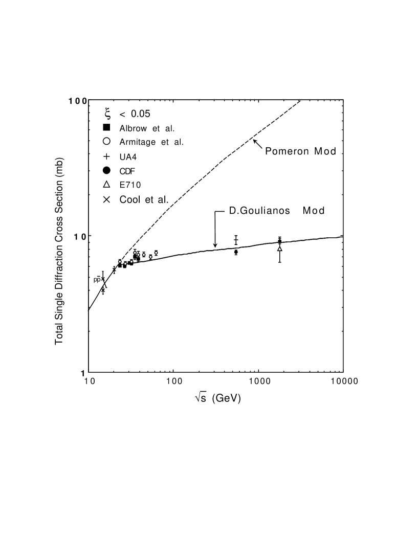
Figure 26: Experimental data on $\sigma_{SD}$ as a function of center mass energy. The dashed curve is the triple-Pomeron prediction while the solid one is one of the model which fits the data. Picture is taken from one of the numerous talks of D. Goulianos.

11 Pomeron in photon - proton interaction.

The photon - hadron interaction has two aspects which makes it quite different from the hadron - hadron interaction ( at least at first sight ). First, the total cross section is of the order of $\alpha_{em}\,\,\approx\,\,1/137\,\,\ll\,\,1$ and, therefore, we can neglect the elastic cross section which is an extra $\alpha_{em}$ times smaller. We need to understand the unitarity constraint here. I Recall that for hadron - hadron collisions the square of scattering amplitude enters the unitarity constraint. Second, we have a unique way to study the dependence of the cross section on the mass of the incoming particle by changing the virtuality of photon. As is well known at large virtualities we are dealing with deep inelastic scattering ( DIS ) which has a simple partonic interpretation. I would like to remind you that DIS will be a subject of the third and fourth parts of my lectures, if any. Here, let us try to understand how to incorporate the Reggeon exchange for photon - proton interaction at high energies.

Figure 27: Two stages of photon - hadron interaction at high energy.

11.1 Total cross section.

Gribov was the first one to observe that a photon ( even virtual one) fluctuates into a hadron system with life time ( coherence length ) $\tau\,\,=\,\,l_{c}\,\,=\,\,\frac{1}{mx_{B}}$ where $x_{B}=\frac{Q^{2}}{s}$, $Q^{2}$ is the photon virtuality and $m$ is the mass of the target. This life time is much larger at high energy than the size of the target and therefore, we can consider the photon - proton interaction as a processes which proceeds in two stages:

(1) Transition $\gamma^{*}\,\rightarrow\,hadrons$ which is not affected by the target and, therefore, looks similar to electron - positron annihilation;

and

(2) $hadron\,\,-\,\,target$ interaction, which can be treated as standard hadron - hadron interaction, for example, in the Pomeron ( Reggeon ) exchange approach ( see Fig.27).

These two separate stages of the photon - hadron interaction allow us to use a dispersion relation with respect to the masses $M$ and $M^{\prime}$ ( Gribov, 1970) to describe the photon - hadron interaction ( see Fig.28a) for notation ), as the correlation length $l_{c}=\frac{1}{mx}\,\gg\,R_{N}$, the target size. Based on this idea we can write a general formula for the photon - hadron interaction,

$$\sigma(\gamma^{*}N)\,\,=\,\,\frac{\alpha_{em}}{3\,\pi}\,\int\frac{\Gamma(M^{2})\,\,d\,M^{2}}{\,Q^{2}\,+\,M^{2}\,}\,\,\sigma(M^{2},M^{\prime 2},s)\,\,\frac{\Gamma(M^{\prime 2})\,\,d\,M^{\prime 2}}{\,Q^{2}\,+\,M^{\prime 2}\,}\,\,.$$ (85)

where $\Gamma(M^{2})=R(M^{2})$ (see Eq. (87) ) and $\sigma(M^{2},M^{\prime 2},s)$ is proportional to the imaginary part of the forward amplitude for $V\,+\,p\,\rightarrow\,V^{\prime}\,+\,p$ where $V$ and $V^{\prime}$ are the vector states with masses $M$ and $M^{\prime}$. For the case of the diagonal transition ( $M=M^{\prime}$) $\sigma(M^{2},s)$ is the total cross section for $V-p$ interaction. Experimentally, it is known that a diagonal coupling of the Pomeron is stronger than an off-diagonal coupling. Therefore, in first approximation we can neglect the off-diagonal transition and substitute in Eq. (85) $\sigma(M^{2},M^{\prime 2},s)\,=\,\sigma)M^{2}.s)\,M^{2}\,\,\delta(\,M^{2}\,-\,M^{\prime 2})$.

Figure 28-a: The generalized Gribov’s formula for DIS.

The resulting photon - nucleon cross section can be written written as:

$$\sigma(\gamma^{*}N)\,\,=\,\,\frac{\alpha_{em}}{3\,\pi}\,\int\frac{R(M^{2})\,M^{2}\,d\,M^{2}}{(\,Q^{2}\,+\,M^{2}\,)^{2}}\,\sigma_{M^{2}N}(s)\,\,,$$ (86)

where $R(M^{2})$ is defined as the ratio

$$R(M^{2})\,\,=\,\,\frac{\sigma(e^{+}e^{-}\,\rightarrow\,hadrons)}{\sigma(e^{+}e^{-}\,\rightarrow\,\mu^{+}\mu^{-})}\,\,.$$ (87)

The notation is illustrated in Fig.28 where $M^{2}$ is the mass squared of the hadronic system, $\Gamma^{2}(M^{2})\,=\,R(M^{2})$ and $\sigma_{M^{2}N}(s)$ is the cross section for the hadronic system to scatter off the nucleonic target.

Figure 28-b: Gribov’s formula for DIS.

In Fig.29 one can see the experimental data for $R(M^{2}=s)$. It is clear that $R(M^{2})$ can be described in a two component picture: the contribution of resonances such as $\rho,\omega,\phi$, J/$\Psi$, $\Psi^{\prime}$ and so on and the contributions from quarks which give a more or less constant term but it changes abruptly with every new open quark - antiquark channel, $R(M^{2})\,\approx\,3\,\sum_{q}\,e^{2}_{q}$, whetre $e_{q}$ is the charge of the quark and the summation is done over all active quark team.

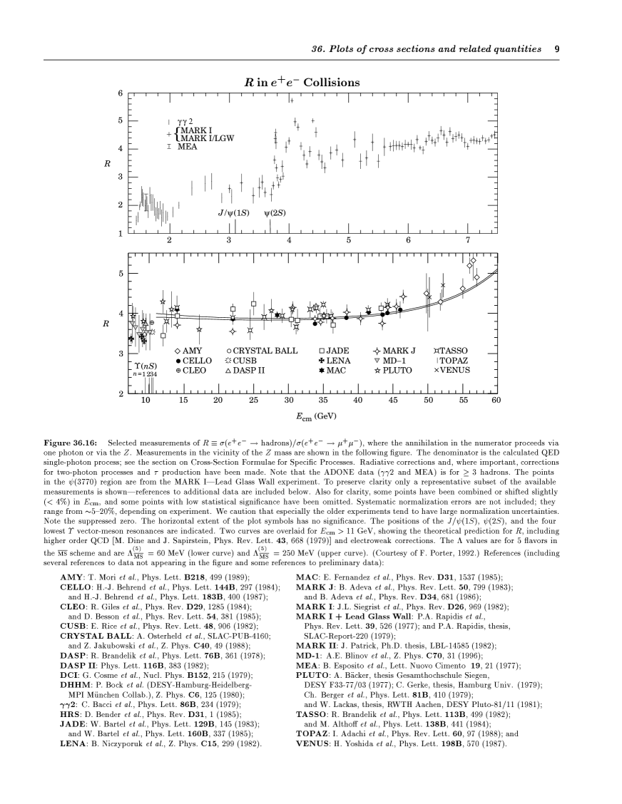
Figure 28-c: Experimental behaviour of $R(M^{2}=E^{2}_{cm})$ ( Particle Data Group 1996 ).

For $\sigma_{M^{2}N}$ we can use the Reggeon exchange approach which gives for the total cross section Eq. (74) where only the vertices $g_{P}$ and $g_{R}$ depend on $M^{2}$.

If we take into account only the contribution of the $\rho$ - meson, $\omega$ - meson , $\phi$ and J/$\Psi$ resonances in $R(M^{2})$ we obtain the so called vector dominance model (VDM) ( J.J. Sakurai 1969) which gives for the total cross section the following formula:

$$\sigma_{tot}(\gamma^{*}\,+\,p\,)\,\,=\,\,\frac{\alpha_{em}}{3\pi}\,\,\sigma_{tot}(\rho+p)\sum_{i}\,\,R(M^{2}=m^{2}_{V_{i}})\{\,\frac{m^{2}_{V_{i}}}{Q^{2}\,\,+\,\,m^{2}_{V_{i}}}\,\}^{2}\,\,$$ (88)

where $m_{V_{i}}$ is the mass of vector meson, $Q^{2}$ is the value of the photon virtuality and $R(M^{2}=m^{2}_{V_{i}})$ is the value of the $R$ in the mass of the vector meson which can be rewritten through the ratio of the electron - positron decay width to the total width of the resonance. Of course, the summation in Eq. (88) can be extended to all vector resonances ( Sakurai and Schildknecht 1972) or even we can return to a general approach of Eq. (85) and write a model for the off-diagonal transition between the vector meson resonances with different masses ( Schildknecht et al. 1975). We have two problems with all generalization of the VDM: (i) a number of unknown experimentally values such as masses and electromagnetic width of the vector resonances with higher masses than those that have been included in VDM and (ii) a lack of theoretical constraints on all mentioned observables. These two reasons give so much freedom in fitting of the experimental data on photon - hadron interaction that it becomes uninteresting and non - instructive.

One can see from Eq. (88), that if $Q^{2}\,\gg\,m^{2}_{V}$ VDM predicts a $\frac{1}{Q^{4}}$ behaviour of the total cross section. Such a behaviour is in clear contradiction with the experimental data which show an approximate $\frac{1}{Q^{2}}$ dependence at large values of $Q^{2}$ ( i.e. scaling ). It should be stressed that the background contribution to Eq. (86) can explain the experimental $Q^{2}$ - dependence. Indeed, for $M^{2}\,\,\gg\,\,m^{2}_{\rho}$ $R(M^{2})\,\,\approx\,\,2$, (see Fig.29). Assuming that $\sigma_{M^{2}N}$ does not depend on $M^{2}$, we have

$$\sigma_{tot}(\gamma^{*}\,+\,p\,)\,\,=\,\,\frac{\alpha_{em}}{3\pi}\,\,\sigma_{tot}(\rho+p)\,\,2\,\,\ln(\frac{Q^{2}\,+\,M^{2}_{0}}{Q^{2}\,+\,m^{2}_{\rho}})\,\,,$$ (89)

where $M_{0}$ is the largest mass up to which we can consider that $\sigma_{M^{2}N}$ is independent of $M^{2}$. Directly from Eq. (89) one can see that

$$\sigma_{tot}(\gamma^{*}\,+\,p\,)\,\,=\,\,\frac{2\,\alpha_{em}}{3\pi}\,\,\sigma_{tot}(\rho+p)\,\,\frac{M^{2}_{0}\,-\,m^{2}_{\rho}}{Q^{2}}\,\,.$$

The value of $M_{0}$ is the new scale of our approach which separates the “soft” ( long distance ) processes from the “hard” ( short distance ) ones. Actually, any discussion of this problem is out of the schedule of these lectures and I want only to point out that QCD leads to the cross section which decreases as $\frac{1}{M^{2}}$ at large $M^{2}$.

In order to write explicitly the Pomeron ( Reggeon ) contribution to the photon - nucleon cross section we have to specify the energy variable. Assume, that the energy variable $s/M^{2}$ will be familiar to the readers.

The contribution of the Pomeron as well as of any Reggeon to photon - nucleon scattering has the following form:

$$\sigma(\gamma^{*}N)\,\,=\,\,\frac{\alpha_{em}}{3\,\pi}\,\int\frac{R(M^{2})\,M^{2}\,d\,M^{2}}{(\,Q^{2}\,+\,M^{2}\,)^{2}}\,g_{P}(M^{2})g^{N}_{P}\,\,(\,\frac{s}{M^{2}})^{\alpha_{P}(0)\,\,-\,\,1}\,\,.$$ (90)

A very important feature of Eq. (90)is the fact that the mass dependence is concentrated only in the dependence of vertex $g_{P}(M^{2})$ and in the energy variable $s/M^{2}$. It is interesting to note that the integral over $M^{2}$ converges even if $g_{P}(M^{2})$ is independent of $M^{2}$. Note also, that at large $M^{2}$ we are dealing with short distance physics where the powerful methods of perturbative QCD have to be applied.

11.2 Diffractive dissociation

Diffractive dissociation is the process which has a large rapidity gap in the final state (see Fig.30). This process can be described using the same approach as in Eq. (86), namely, the dispersion relation with respect to $M^{2}$ in Fig.30. However, it is useful to discuss separately two cases: the exclusive final state with a restricted number of hadrons and inclusive diffraction dissociation without any selection in the final state. To understand the difference between these two cases, recall, that, according to the second definition of the Pomeron, the typical final state in diffractive processes is still the parton “ladder”, namely, the final state hadrons are uniformly distributed in rapidity. In other words for a fixed but large mass $M$ of the final state the typical multiplicity of the produced hadrons $N\,\propto\,a\ln M^{2}$, where $a$ is the particle density in rapidity ( the number of particles per unit rapidity interval). Therefore, the final state with a fixed number of hadrons ( partons ) has a suppression which is proportional to $\exp(-a\,\ln M^{2})$. Hence for the exclusive process with fixed number of hadrons in the final state one has to find a new mechanism different from the normal partonic one. This mechanism is rather obvious since the large value of $M$ can be due to a large value of the parton ( hadron ) transverse momenta ( $k_{it}$ in the final state which are of the order of $M$ ( $k^{2}_{it}\,\approx\,M^{2}$ ). Concluding this introduction to the DD processes in Reggeon approach, we emphasize that

(i) for exclusive final states with a fixed number of hadrons (partons) the large diffractive mass originates from the parton ( hadron ) interaction at small distances;

(ii) while the inclusive DD in the region of large mass looks like a normal inclusive process in the parton model with a uniform distribution of the secondary hadrons in rapidity and with a limited hadron transverse momentum which does not depend on $M$.

11.3 Exclusive ( with restricted number of hadrons) final state.

For this process we can use Gribov’s formula ( see Fig.30 ). Futhermore, for large values of the mass one can calculate the transition from the virtual photon to a quark - antiquark pair in perturbative QCD. So, here, for the first time in my lecture I recall our microscopic theory - QCD, but, actually, we will discuss here only a very simple idea of QCD, namely, the fact that the correct degrees of freedom are quark and gluons.

Figure 29: Gribov’s formula for diffractive dissociation (DD) in DIS.

Let us start with the definition of the variables:

1. The Bjorken $x$ variable is given by

$$x_{B}\,\,=\,\,x\,\,=\,\,\frac{Q^{2}}{s}\,\,,$$

where $s$ is the square of the total c.m. energy of the virtual photon - proton system and $Q^{2}$ is the photon virtuality;

2. As usual, we introduce

$$x_{P}\,\,=\,\,\frac{Q^{2}\,\,+\,\,M^{2}}{Q^{2}\,\,+\,\,s}\,\,,$$

which is the fraction of the proton energy carried by the Pomeron;

3. $\beta\,\,=\,\,\frac{Q^{2}}{Q^{2}\,\,+\,\,M^{2}}\,\,=\,\,\frac{x_{B}}{x_{P}}\,\,,$ where $\beta$ is the fraction of the Pomereon energy carried by the struck parton in the Pomeron;

4. The transverse momenta of the out going quark and antiquark are denoted by $\pm\,\,\vec{k}_{t}$, and those of the exchanged partons ( gluons) by $\pm\,\,\vec{l}_{t}$;

5. It is convenient to use light - cone perturbation theory and to express the particle four momenta in the form:

$$k_{\mu}\,\,=\,\,(\,k_{+},k_{-},\vec{k}_{t}\,)\,\,,$$

where $k_{\pm}\,\,=\,\,k_{0}\,\,\pm\,\,k_{3}$;

6. In the frame in which the target is essentially at rest we have

$$q_{\mu}\,\,=\,\,(\,q_{+},-\,\frac{Q^{2}}{q_{+}},\vec{0}_{t}\,)\,\,;$$

$$k_{\mu}\,\,=\,\,(\,k_{+},-\,\frac{m^{2}_{t}}{k_{+}},\vec{k}_{t}\,)\,\,;$$

$$l_{\mu}\,\,=\,\,(\,l_{+},-\,\frac{l^{2}_{t}}{l_{+}},\vec{l}_{t}\,)\,\,;$$

with $m^{2}_{t}\,\,=\,\,m^{2}_{Q}\,\,+\,\,k^{2}_{t}$ where $m$ is the quark mass. $q_{\mu}$ is the four momentum of the photon ($q^{2}\,\,=\,\,-\,Q^{2}$).

The Gribov factorization ( Gribov’s formula ) follows from the fact that the time of quark - antiquark fluctuation $\tau_{\gamma^{*}}$ is much longer than the time of interaction with partons ($\tau_{i}$ ). It is instructive to illustrate why this is so. According to the uncertainty principle the fluctuation time is equal to:

$$\tau_{\gamma^{*}}\,\,\sim\,\,|\,\frac{1}{q_{-}\,\,-\,\,k_{1-}\,\,-\,\,k_{2-}}\,|\,\,=\,\,\frac{q_{+}}{Q^{2}\,\,+\,\,M^{2}}\,\,,$$ (91)

where $k_{1}$ and $k_{2}$ are four momenta of the quarks of mass $m$, and

$$M^{2}\,\,=\,\,\frac{m^{2}\,\,+\,\,k^{2}_{t}}{z(1\,-\,z)}\,\,.$$

To estimate the interaction time we calculate the typical time of the emission of a parton with momentum $l_{\mu}$ from quark $k_{1}$, which is

$$\tau_{i}\,\,=\,\,|\,\frac{1}{k_{1-}\,\,-\,\,k^{\prime}_{1-}\,\,-\,\,l_{-}}\,|\,\,=\,\,|\,\frac{q_{+}}{\frac{m^{2}_{t}}{z}\,\,-\ ,\,\frac{m^{2}_{t}}{z^{\prime}}\,\,-\,\,\frac{l^{2}_{t}}{\alpha}}\,|\,\,,$$ (92)

where $\alpha\,=\,\frac{l_{+}}{q_{+}}$ and $z^{\prime}\,=\,z\,-\,\alpha$. In leading log $s$ approximation in which we have obtained the Pomeron, we have $\alpha\,\,\ll\,\,z$ and hence

$$\tau_{i}\,\,=\,\,\frac{\alpha q_{+}}{l^{2}_{t}}\,\,\ll\,\,\tau_{\gamma^{*}}\,\,.$$

Therefore, we can write Gribov’s formula as it is given in Fig.30, namely:

$$M(\,\,\gamma^{*}\,+\,p\,\,\,\rightarrow\,\,\,M^{2}\,+\,\,[\,LRG\,]\,\,+\,\,p\,\,)\,\,=$$ (93)

$$\,\,\int\,d^{2}k_{t}\,\int^{1}_{0}\,dz\,\Psi^{\gamma^{*}}(z,k_{t},Q)\,A_{P}(M^{2},s)\,\,\Psi_{final}(\bar{q}q\rightarrow hadrons)\,\,,$$

where LRG stands for “large rapidity gap”.

The wave function of the virtual photon can be written in the following way:

$$\Psi^{\gamma^{*}}(z,k_{t},Q)\,\,\,=\,\,\,-eZ_{f}\,\frac{\bar{u}(k_{t},z)\,\gamma\cdot\epsilon\,v(-k_{t},1-z)}{\sqrt{z(1\,-\,z)}}\,\frac{1}{Q^{2}\,\,-\,\,M^{2}}\,\,,$$ (94)

where $\vec{\epsilon}$ is the photon polarization: for longitudinal polarized photon we have

$$\epsilon_{L}\,\,=\,\,(\,\frac{q_{+}}{Q},\frac{Q}{q_{+}},\vec{0}_{t}\,)$$

while for transverse polarized photons ($\vec{\epsilon}_{t}$) we will use as basis the circular polarization vectors :

$$\epsilon_{\pm}\,\,=\,\,\frac{1}{\sqrt{2}}\,(\,0,0,1,\pm i\,)\,\,.$$

To evaluate Eq. (94) with $\epsilon\,=\,\epsilon_{L}$ we first note that

$$q^{\mu}\,\bar{u}\gamma_{\mu}v\,\,=\,\,\frac{1}{2}\,(\,q_{+}\bar{u}\gamma_{-}v\,\,+\,\,q_{-}\,\bar{u}\gamma_{+}v\,)\,\,=\,\,0$$

and therefore

$$\bar{u}\gamma_{-}v\,\,=\,\,\frac{Q^{2}}{q^{2}_{+}}\,\bar{u}\gamma_{+}v\,\,.$$

We can use this identity to evaluate the wave function:

$$\bar{u}\gamma\cdot\epsilon_{L}v\,\,=\,\,\frac{1}{2}\,\{\,\frac{q_{+}}{Q}\bar{u}\gamma_{-}v\,\,+\,\,\frac{Q}{q_{+}}\bar{u}\gamma_{+}v\,\}\,\,=\,\,\frac{Q}{q_{+}}\bar{u}\gamma_{+}v\,\,=\,\,2Q\sqrt{z(1\,-\,z)}\delta_{\lambda,-\lambda^{\prime}}\,\,,$$

where $\lambda$ is helicity of the antiquark while $\lambda^{\prime}$ is the helicity of the quark ( we omitted helicities in most of the calculations but put them correctly in the answer). Coming back to Eq. (94) one can see that:

$$\Psi^{\gamma^{*}}_{L}\,\,=\,\,-eZ_{f}\,\frac{4\,Q\,\delta_{\lambda,-\lambda^{\prime}}}{Q^{2}\,\,+\,\,M^{2}}\,\,.$$ (95)

For the transverse polarized photons with helicity $\lambda_{\gamma}\,\,=\,\,\pm 1$ one finds:

$$\Psi^{\gamma^{*}}_{T}\,\,=\,\,-eZ_{f}\,\frac{\delta_{\lambda,-\lambda^{\prime}}\,\{(\,1\,-\,2z\,)\lambda_{\gamma}\,\pm\,1\,\}\,\vec{\epsilon}_{\pm}\cdot\vec{k}_{t}\,\,+\,\,\delta_{\lambda,\lambda^{\prime}}\,m\,\lambda_{\gamma}}{[z(1\,-\,z]\,\,\,\,\,\,(Q^{2}\,\,+\,\,M^{2}\,)}\,\,.$$ (96)

To obtain the expression for the diffractive dissociation cross section we have to square the amplitude and sum over all quantum numbers of the final state ( with fixed mass $M$ ). Assuming that experimentally no selection has been made or in other words $\Psi_{finaL}$ does not describe a specific state with definite angular momentum, we can sum over helicities and obtain the following answers:

$$\frac{d\sigma^{SD}_{L}}{dM^{2}dt}\,\,=\,\,\frac{\alpha_{em}}{48\pi^{3}}\frac{Q^{2}R^{exclusive}_{L}(M^{2})}{\{\,Q^{2}\,\,+\,\,M^{2}\,\}^{2}}g^{2}_{P}(M^{2})g^{2}_{p}\,(\,\frac{s}{Q^{2}\,+\,M^{2}}\,)^{2\Delta}\,\,;$$ (97)

$$\frac{d\sigma^{SD}_{T}}{dM^{2}dt}\,\,=\,\,\frac{\alpha_{em}}{48\pi^{3}}\frac{M^{2}R^{exclusive}_{T}(M^{2})}{\{\,Q^{2}\,\,+\,\,M^{2}\,\}^{2}}g^{2}_{P}(M^{2})g^{2}_{p}\,(\,\frac{s}{Q^{2}\,+\,M^{2}}\,)^{2\Delta}\,\,;$$ (98)

where $R_{L,T}(M^{2})$ is defined as the ratio

$$R_{L,T}(M^{2})\,\,=\,\,\frac{\sigma(e^{-}+e^{+}\,\rightarrow\,hadrons\,with\,mass\,M)}{\sigma(e^{-}e^{+}\,\rightarrow\,\mu^{-}\mu^{+})}\,\,.$$

Eq. (97) and Eq. (98) give us the possibility to measure experimentally the dependence of $g(M^{2})$ on $M$ and therefore to determine the value of the separation scale $M_{0}$. As we have discussed, this scale separates the long distance ( nonperturbative, “soft” ) physics from the short distance one ( perturbative, “hard”). It is hardly necessary to mention how important this information for our understanding of the nonperturbative QCD contribution in orde5r to find a way out of the Reggeon phenomenology.

11.4 Inclusive diffraction

Diffractive production of a large mass in $\gamma^{*}p$ scattering in the Reggeon approach looks quite similar to diffractive dissociation in hadron - hadron collisions. We can safely apply the triple Reggeon phenomenology and the formulae have the same form as Eq. (76), namely

$$\frac{M^{2}d\sigma_{SD}(\gamma^{*}p)}{dM^{2}}\,\,=\,\,\frac{\sigma_{0}}{2\pi R^{2}(\frac{s}{M^{2}})}\,\cdot\,(\frac{s}{M^{2}})^{2\Delta}\,\cdot\,[\,g^{\gamma^{*}}_{P}\cdot G_{3P}(0)\,\cdot\,(\frac{M^{2}}{s_{0}})^{\Delta}\,+\,\,g^{\gamma^{*}}_{R}\cdot G_{PPR}(0)(\frac{M^{2}}{s_{0}})^{\alpha_{R}(0)-1}\,]\,\,.$$ (99)

There is only one difference , namely, we can apply Gribov’s formula for the vertex $g^{\gamma^{*}}_{P,R}$. Indeed,

$$g^{\gamma^{*}}_{P,R}(Q^{2})\,\,=\,\,\frac{\alpha_{em}}{3\,\pi}\,\int^{M^{2}_{0}}\frac{R(M^{\prime 2})M^{\prime 2}dM^{\prime 2}}{(\,Q^{2}\,+\,M^{\prime 2}\,)^{2}}\,\,g_{P,R}(M^{2})\,(\,\frac{s_{0}}{M^{\prime 2}}\,)^{\alpha_{P,R}(0)\,-\,1}\,\,.$$ (100)

We introduce explicitly the separation scale $M_{0}$ to demonstrate that we trust this formula only in the region of sufficiently small masses while at large masses this integral should be treated in perturbative QCD.

Notice that the $Q^{2}$ dependence is concentrated only in the vertex $g^{\gamma^{*}}_{P,R}$ and, therefore, one of the predictions of the Pomeron approach is that large mass diffraction has the same $Q^{2}$ dependence as the total $\gamma^{*}p$ cross section. Surprisingly the HERA data are not in contradiction with this prediction.

However, it should be stressed that the Pomeron approach can be trusted only for rather small virtualities while at large $Q^{2}$ perturbative QCD manifests itself as more powerful and reliable tool for both the DIS total cross sections and diffractive dissociation in DIS. The challenge for everybody who is trying to understand the photon - hadron interaction is to find the region of applicability of pQCD and to separate “soft” and “ hard” interactions. This task is impossible without a certain knowledge of the Reggeon phenomenology.

12 Shadowing Corrections ( a brief outline ).

12.1 Why is the Pomeron not sufficient?

I hope, that I have given a lot of information on the Reggeon phenomenology. Now, I want to touch several difficult and important topics and, in particular, I want to explain why the Pomeron hypothesis is not sufficient. A full discussion of these tropics will be given in the second part of my lectures, but I would like to give here a brief review of the shadowing corrections (SC) properties to discuss the experimental way of studying the Pomeron structure which I will present in the next section.

Firstly, the hypothesis that the Pomeron gives the asymptotic behaviour of the scattering amplitude is not correct. To illustrate this fact let us consider single diffraction dissociation in the region of large mass $M$ ( see Fig.23c). In this kinematic region we can apply the triple Pomeron formula for the cross section. Using Eq.(76b) and the exponential parameterization for the $t$ - dependence of all vertices, leads to the following expression for the single diffraction cross section:

$${SDSC}\frac{M^{2}d^{2}\sigma_{SD}}{dM^{2}\,dt}\,\,=\,\,(g^{p}_{P}(0))^{3}\cdot G_{PPP}(0)\cdot e^{2(R^{2}_{0}+r^{2}_{0}+\alpha^{\prime}_{P}\ln(s/M^{2}))t}\,(\,\frac{s}{M^{2}}\,)^{2\,\Delta_{P}}\,(\,\frac{M^{2}}{s_{0}}\,)^{\Delta_{P}}\,\,,$$ (101)

where $R^{2}_{0}$ and $r^{2}_{0}$ give the $t$-dependence of the Pomeron - proton form factor and the triple Pomeron vertex respectively. The total diffractive dissociation cross section for large masses $M$ ( $M\,\geq\,M_{0}$) is given by:

$$\sigma_{SD}(M\,\geq\,M_{0})\,\,=$$ (102)

$$\int^{0}_{-\infty}\,dt\int^{s}_{M^{2}_{0}}\,dM^{2}\frac{d^{2}\sigma_{SD}}{dM^{2}\,dt}\,\,=\,\,\frac{(g^{p}_{P}(0))^{3}\cdot G_{PPP}(0)}{2(R^{2}_{0}+r^{2}_{0}+\alpha^{\prime}_{P}\,\ln(s/M^{2}_{0})}\cdot(\,\frac{s^{2}}{s_{0}M^{2}_{0}\,})^{\Delta_{P}}\,\,.$$

One sees that $\sigma_{sd}\,\propto\,s^{2\Delta_{P}}$ while the total cross section is proportional to $s^{\Delta_{P}}$. It means that something is deeply wrong in our approach which can lead to a cross section for diffractive dissociation which is larger than the total cross section. For $\Delta_{P}\,>\,0$ we can take a simpler example like the elastic cross section or the cross section of diffractive dissociation in the region of small masses ($M\leq M_{0}$ ). What is important is the fact that the diffractive dissociation at large masses leads to a cross section which increases with energy even if $\Delta_{P}=0$. Indeed, repeating all calculations in Eq. (102) for $\Delta_{P}=0$ we can see that

$$\sigma_{SD}\,\,\propto\,\,\ln\ln s\,\,\gg\,\,\sigma_{tot}\,\,\propto\,\,Const\,\,.$$

The way out is to take into account the interaction between Pomerons, in particular with the triple Pomeron vertex. I will postpone this problem to the second part of the lectures. I would like to show here that the interactions between Pomerons and with particles is a natural outcome of the parton space - time picture that we have discussed in section 8.

12.2 Space - time picture of the shadowing corrections.

To understand, why we have to deal with the SC, we have to look back at Figs.21e and 21f. When I discussed these pictures in sections 8.2 and 8.3, I cheated a bit or rather I did not stress that we had made the assumption that only one “wee” parton interacts with the target. Now, let ask ourselves why only one? What is going to happen if, let us say, two “wee” partons interact with the target? Look, for example, at Fig. 21e. If two “wee” partons interact with the target the coherence in two “ladders” will be destroyed. Squaring this amplitude with two incoherent “ladders”, one can see that we obtain the diagram in which two initial hadrons interact by the exchange of two Pomerons. Here, I used the second definition of the Pomeron, namely, Pomeron = “ladder”.

Therefore, the whole picture of interaction looks as follows. The fast hadron decays into a large number of partons and this partonic fluctuation lives for a long time $t\,\propto\,\frac{E}{\mu^{2}}$ ( see Fig.21d ). During this time each parton can create its own chain of partons and, as we have discussed, results in the production of $N$ “wee’ partons, which can interact with the target with a standard cross section ( $\sigma_{0}$ ). Assuming that only one “wee” parton interacts with the target we obtained Eq.(72), namely, $\sigma^{P}_{tot}\,=\,\sigma_{0}\cdot N$. This process we call the Pomeron exchange.

However, several “wee” partons can interact with the target. Let us assume that two “wee” partons interact with the target. The cross section will be equal to $\sigma^{P}_{tot}\cdot W$, where $W$ is the probability for the second “wee” parton to meet and interact with the target. As we have discussed in section 7.4 all “wee” partons are distributed in an area in the transverse plane which is equal $\pi R^{2}(s)$ and $R^{2}\,\,\rightarrow\,\,\alpha^{\prime}_{P}\ln(s)$. Therefore, the cross section of the two “wee” parton interaction is equal to

$$\sigma^{(2)}\,\,=\,\,\sigma_{0}\cdot N\cdot\frac{\sigma_{0}\cdot N}{\pi R^{2}(s)}\,\,.$$ (103)

If $\Delta_{P}\,>\,0$ this cross section tends to overshoot the one “wee” parton cross section. However, if $\Delta=0$ $\sigma^{(2)}$ turns to be much smaller than $\sigma^{P}_{tot}$, namely,

$$\sigma^{(2)}\,\,=\,\,\frac{(\,\sigma^{P}_{tot}\,)^{2}}{\pi\,R^{2}(s)}\,\,.$$ (104)

Remember that Eq. (104) had given us the hope that the Pomeron hypothesis will survive. However, let me recall that the problem with the triple Pomeron interaction and with the large mass diffraction dissociation as the first manifestation of such an interaction remains even if $\Delta_{P}=0$.

Now let us ask ourselves what should be the sign for a $\sigma^{(2)}$ contribution to the total cross section. A strange question, isn’t it. My claim is that the sign should be negative. Why? Let us remember that the total cross section is just the probability that an incoming particle has at least one interaction. Therefore, our interaction in the parton model is the probability for the scattering of the flux of $N$ “wee” partons with the target. To calculate the total cross section we only need to insure that at least one interaction has happened. However, we overestimate the value of the total cross section since we assumed that every parton out of the total number of “wee” partons $N$ is able to interact with the target. Actually, the second parton cannot interact with the target if it is just behind the first one. The probability to find the second parton just behind the first one is equal to $W$ which we have estimated. Therefore, the correct answer for the flux of “wee” partons that can interact with the target is equal to

$$FLUX\,\,=\,\,N\cdot(\,1\,-\,W\,)\,\,=\,\,N\cdot(\,1\,-\,\frac{\sigma^{P}_{tot}}{\pi R^{2}(s)}\,)\,\,$$

which leads to the total cross section:

$$\sigma_{tot}\,\,=\,\,\sigma^{P}_{tot}\,\,-\,\,\frac{(\,\sigma^{P}_{tot}\,)^{2}}{\pi R^{2}(s)}\,\,.$$ (105)

I hope that everybody recognizes the famous Glauber formula.

Therefore,the shadowing corrections for Pomeron exchange is the Glauber screening of the flux of “wee” partons.

If $W\,\,\ll\,\,1$ we can restrict ourselves to the calculation of interactions of two “wee” partons with the target. However, if $W\,\approx\,1$ we face a complicated and challenging problem of calculating all SC. We are far away from any solution of this problem especially in the “soft’ interaction. Here, I am only going to demonstrate how the SC works and what qualitative manifestation of the SC can be expected in high energy scattering.

12.3 The AGK cutting rules.

The Abramovsky - Gribov - Kancheli ( AGK ) cutting rules give the generalization of the optical theorem for the case of multi - Pomeron exchange.

Indeed, the optical theorem for one Pomeron exchange ( $\sigma^{(1)}_{1}$ in Fig. 32 ) decodes the Pomeron structure and says that the Pomeron contribution to the total cross section is closely related to the cross section for the production of a large number of hadrons ( partons) $<n_{P}>$ which in first approximation are uniformly distributed in rapidity (Feynman gas hypothesis).

In the case of a two “wee” parton interaction or, in other words, in the case of two Pomeron exchange there are three different contributions to the total cross section if we analyze them from the point of view of the type of the inelastic events.

They are ( see Fig.32 ):

1. The diffractive dissociation ( $\sigma^{(0)}_{2}$ ) processes which produces a very small multiplicity of the particles in the final state. A clear signature of these processes is the fact that no particles are produced in the large gap in rapidity ( see Fig.32 and the lego - plot for $\sigma^{(0)}_{2}$ typical event).

2. The production of secondary hadrons with the same multiplicity as for one Pomeron exchange ( see $\sigma^{(1)}_{2}$ in Fig.32 ). This event has the same multiplicity ( $<n_{P}>$) as the one Pomeron exchange ( compare $\sigma^{(1)}_{2}$ with $\sigma^{(1)}_{1}$ in Fig.32 ).

3. The production of secondary hadrons with a multiplicity which is twice as large as for one Pomeron exchange ( see $\sigma^{(2)}_{2}$ in Fig.32 ).

The AGK cutting rules claim :

$$\sigma^{(0)}_{2}\,\div\,\sigma^{(1)}_{2}\,\div\,\sigma^{(2)}_{2}\,\,=\,(\,1\,)\,\div\,(\,-4\,)\,\div\,(\,2\,)$$ (106)

Two important consequences follow from the AGK cutting rules:

1. The total cross section of diffraction dissociation (DD) is equal to the contribution of two Pomeron exchange to the total cross section ( $\sigma^{(2P)}_{tot}$ ) with opposite sign:

$$\sigma^{(DD)}\,\,=\,\,-\,\sigma^{(2P)}$$

2. The two Pomeron exchange does not contribute to the total inclusive cross section in the central kinematic region. Indeed only two processes, $\sigma^{(1)}$ and $\sigma^{(2)}$, are sources of particle production in the central region. Therefore, the total inclusive cross section due to two Pomeron exchange is equal to

$$\sigma_{inc}\,=\,\sigma^{(1)}\,+\,2\,\sigma^{(2)}\,=\,0$$

The factor 2 comes from the fact that the particle can be produced from two different parton showers ( see $\sigma^{(2)}_{2}$ in Fig. 32).

Figure 30: Hadron - deuteron interaction.

Now let me give you a brief proof of the AGK cutting rules for the case of hadron - deuteron interactions ( see Fig.31). For simplicity let us assume that $G_{in}(b_{t})\,=\,\kappa\,=\,Const(b_{t})$ for $b_{t}<R_{N}$ and $G_{in}=0$ for $b_{t}>R_{N}$. Than the inelastic cross section for hadron - nucleon interaction is equal to

$$\sigma^{inel}_{N}\,=\,\kappa\,S$$

where S is the area of the nucleon ( S = $\pi R^{2}_{N}$ ). To calculate the elastic cross section we need to use the unitarity constraint for $b_{t}$ ( see Eq.(20 ) which leads to

$$\sigma^{el}_{N}\,=\,(\frac{\kappa}{2})^{2}S$$

Noting that the flux of incoming particles after the first interaction becomes $(1-\kappa)$ we can calculate the total inelastic interaction with the deutron

$$\sigma^{inel}_{D}\,\,=\kappa S\,\,+\,\,\kappa(1-\kappa)S\,\,=\,\,2\,\sigma^{inel}_{N}-\kappa^{2}S$$

Imposing the unitarity condition the elastic cross section for the interaction with deuteron is equal to

$$\sigma^{el}_{D}\,\,=\,\,(\frac{2\kappa}{2})^{2}S$$

Note that in the calculation of the elastic cross section we cannot use probabilistic argumentation, we have to use the unitarity constraint of Eq.(20). Therefore the total cross section for hadron - deutron interaction can be presented in the form:

$$\sigma^{tot}_{D}\,\,=2\,\sigma^{tot}_{N}\,-\,\Delta\sigma$$

where

$$\Delta\sigma\,\,=\,\,\Delta\sigma^{inel}\,+\,\Delta\sigma^{el}\,=\,-\,\frac{\kappa^{2}}{2}\,S\,=\,-\,\frac{(\sigma^{inel}_{N})^{2}}{2\pi R^{2}}$$

You will again recognize the Glauber formula for hadron - deutron interactions.

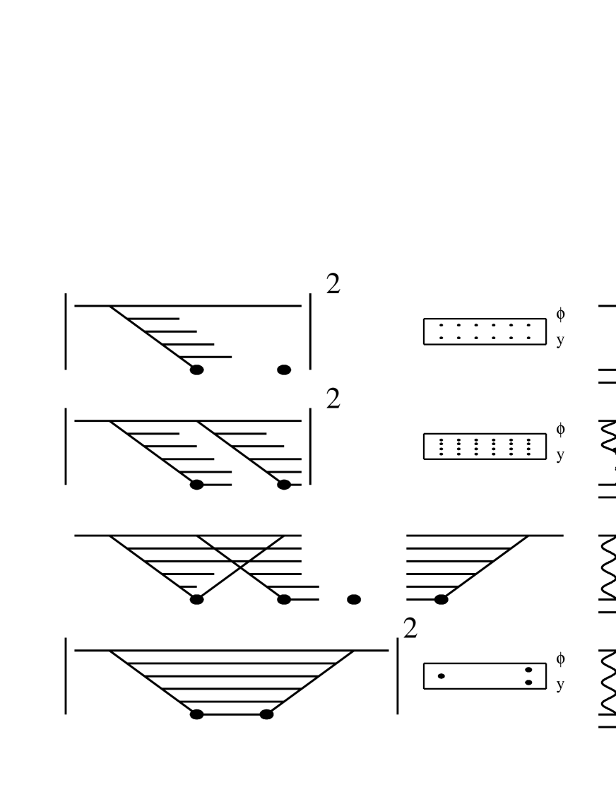
Figure 31: The AGK cutting rules for hadron - deuteron interaction. Dots mark cut Pomerons and particles on mass shell.

As mentioned before there are two sources of the inelastic cross section which are pictured in Fig. 32 for the case of the deutron. The cross section for the inelastic process with doubled multiplicity is easy to calculate, since it is equal to the probability for two inelastic interactions:

$$\Delta\sigma^{(2)}_{2}\,\,=\,\,\kappa^{2}\cdot S$$

To calculate $\sigma^{(1)}_{2}$ we have to remember that

$$\Delta\sigma^{inel}\,\,=\,\,\sigma^{(2)}_{2}\,\,+\,\,\sigma^{(1)_{2}}\,\,=\,\,-\kappa S$$

Therefore $\sigma^{(1)}_{2}\,=\,-2\kappa S$. Since $\Delta\sigma^{(0)}_{2}\,=\,\sigma^{el}_{D}\,-\,2\sigma^{el}_{N}$ we get

n	0	$<n>_{N}$	2$<n>_{N}$
$\Delta\sigma_{tot}$	$\frac{\kappa^{2}}{2}S$	$-2\kappa^{2}S$	$\kappa^{2}S$

Therefore we find the AGK cutting rules for hadron - deuteron interactions, since $\sigma^{tot}_{D}\,=\,2\sigma^{tot}_{N}$ corresponds to one Pomeron exchange and the correction to this simple formula just originated from the two Pomeron exchange in our Reggeon approach. However the above discussion, I hope, shows you that the AGK cutting rules have more general theoretical justification than the Reggeon approach. For example, they hold in QCD providing the so called factorization theorem.

Let me give here the general formula for the AGK cutting rules. The contribution to the total cross section from the exchange of $\nu$ Pomerons ( $\sigma^{\nu}_{tot}$) and the cross sections for the for the production of $\mu<n_{P}>$ particles ( $\sigma^{(\mu)}_{\nu}$ ) which are generated by the same diagram (see Fig.32) are related:

$$\frac{\sigma^{(\mu)}_{\nu}}{\sigma^{\nu}_{tot}}\,|_{\mu\neq 0}\,\,=\,\,(-1)^{\nu-\mu}\cdot\frac{\nu!}{\mu!\,(\nu-\mu)!}\cdot 2^{\nu}$$ (107)

For $\mu=0$ the ratio is equal to

$$\frac{\sigma^{(0)}_{\nu}}{\sigma^{\nu}_{tot}}\,\,=\,\,(-1)^{\nu}\cdot[\,2^{\nu-1}\,-\,1\,]$$ (108)

These factors for exchanging 1,2,…5 Pomerons are given in the following table.

$\nu\setminus\mu$	0	1	2	3	4	5
1	0	1	0	0	0	0
2	1	- 4	2	0	0	0
3	- 3	12	- 12	4	0	0
4	7	- 32	48	- 32	8	0
5	- 15	80	- 160	160	- 80	16

12.4 The Eikonal model.

The simplest way of estimating the value of the SC is the so called Eikonal model. It is easy to understand the Eikonal model from the general solution for $s$-channel unitarity ( see Eq.(26)):

$$a_{el}(s,b)\,\,=\,\,i\,\{\,1\,\,-\,\,e^{-\,\frac{\Omega(s,b)}{2}}\,\,\}\,\,;$$ (109)

$$G_{in}(s,b)\,\,=\,\,1\,\,-\,\,e^{-\,\Omega(s,b)}\,\,.$$ (110)

The weak unitarity constrains are $Im\,a_{el}(s,b)\,\,\leq\,\,1$ and $G_{in}(s,b)\,\,\leq\,\,1$ which follow directly from Eq. (109) and Eq. (110).

At small values of opacity $\Omega$,   $a_{el}\,=\,\Omega/1$ and $G_{in}=\Omega$. Since we assume that the Pomeron is a good approximation until the SC become large, we take $\Omega$ equal to the result for one Pomeron exchange, namely:

$$\Omega(s,b)\,\,=\,\,\frac{\sigma_{0}(s=s_{0})}{\pi R^{2}_{ab}(s)}\cdot(\,\frac{s}{s_{0}}\,)^{\Delta_{P}}e^{-\,\frac{b^{2}}{R^{2}_{ab}(s)}}\,\,,$$ (111)

where $\sigma_{0}$ is the total cross section for $a+b$ scattering at some value of energy ($s=s_{0}$) where we expect the SC to be small. In the exponential parameterization where the $t$ - dependence of the Pomeron - hadron vertex $g^{P}_{a}(t)\,\,=\,\,exp(\,-\,R^{2}_{0a}|t|\,)$

$$R^{2}_{ab}\,\,=\,\,4\cdot(\,R^{2}_{0a}\,\,+\,\,R^{2}_{0b}\,\,+\,\,\alpha^{\prime}_{P}(0)\ln(s/s_{0})\,)\,\,.$$

Certainly, this is an assumption which has no theoretical proof. From the point of view of the parton model this assumption looks very unnatural since the Eikonal model describes the SC induced only by “wee” partons originating from the fastest parton ( hadron ). There is no reason why “wee” partons created by the decay of any parton, not only the fastest one, should not interact with the target. Using $s$ - channel unitarity and our main hypothesis that the Pomeron = “ladder” ( the second definition for the Pomeron ) one can see that the rich structure of the final state simplifies to two classes of events: (i) elastic scattering and (ii) inelastic particle production with a uniform rapidity distribution ( Feynman gas assumption). In particular, we neglected a rich structure of the diffractive dissociation events as well as all of events with sufficiently large rapidity gaps.

In some sense the Eikonal model is the direct generalization of the Feynman gas approach, namely, we take into account the Feynman gas model for the typical inelastic event and for elastic scattering since we cannot satisfy the unitarity constraint without including elastic scattering. As I have discussed the $G_{in}$ in Eq.(20) can be treated almost classically and the probabilistic interpretation for this term can be used. However, the first two terms in Eq.(20), namely $2\,Ima_{el}$ and $|a_{el}|^{2}$, is the quantum mechanics ( optics ) result and both terms must be taken into account.

However, the Eikonal model can be useful in the limited range of energy and the physical parameter which is responsible for the accuracy of calculation in the Eikonal model is the ratio of

$$\gamma\,\,=\,\,\frac{G_{PPP}(0)}{g^{P}_{a}(0)}\,=\,\frac{\sigma_{SD}}{2\sigma_{el}}\,\,.$$

It is interesting to note that in the whole range of energies which are accesible experimentally $\gamma\,\leq 1/4$. Therefore, we can use this model for a first estimate of the value of SC to find the qualitative signature of their influence and to select an efficient experimental way to study SC.

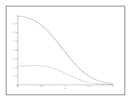
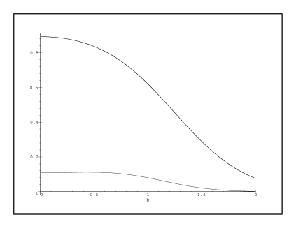
Fig. 34-a	Fig. 34-b
Fig. 34-c	Fig. 34-d

Figure 33: The impact parameter dependence for $G_{in}(s,b)$ and $\Gamma(s,b)$ at two values of energy $\sqrt{s}\,=\,400\,GeV$ ( Fig.34-a and Fig. 34-c) and $\sqrt{s}\,=\,4\,10^{6}\,GeV$ ( Fig. 34-b and Fig. 34-d).

First, let us fix our numerical parameters using the Fermilab data at fixed target energy. We take $s_{0}=400GeV^{2}$, $\sigma_{0}$ = 40 mb, $R^{2}_{0p}=2.6GeV^{-2}$, $\alpha^{\prime}_{P}(0)\,=\,0.25GeV^{-2}$ and $\Delta$ = 0.08. As you can see we take use the parameters of the D-L Pomeron but we use the simple exponential parameterization for vertices while Donnachie and Landshoff used a more advanced $t$-distribution which follows from the additive quark model. In Fig.33 you can see the result of our calculation for: $\Omega(s,b)$, $Im\,a_{el}(s,b)$ and $G_{in}(s,b)$ as function of $b$ at $s=s_{0}$ and at the Tevatron energy.

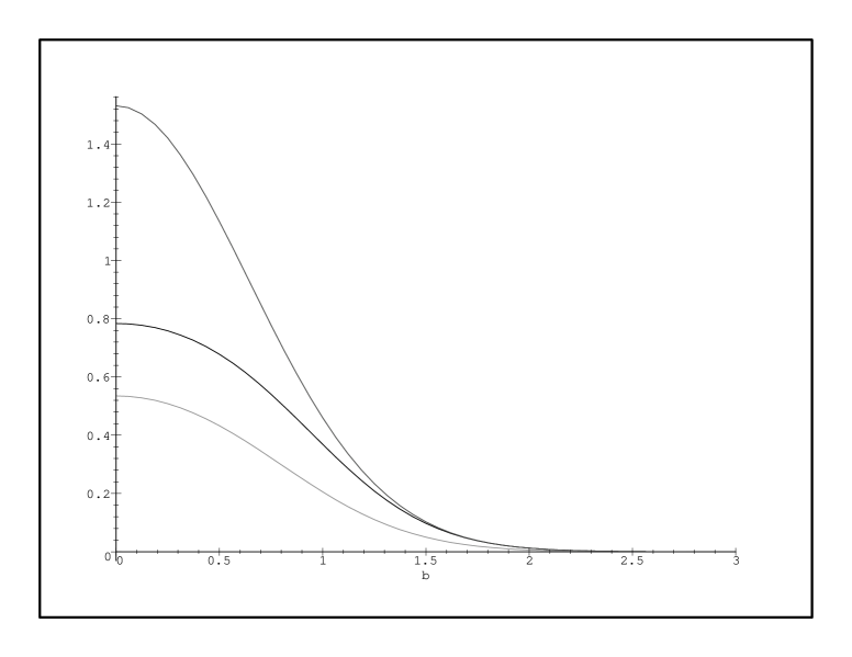
Fig. 33-a

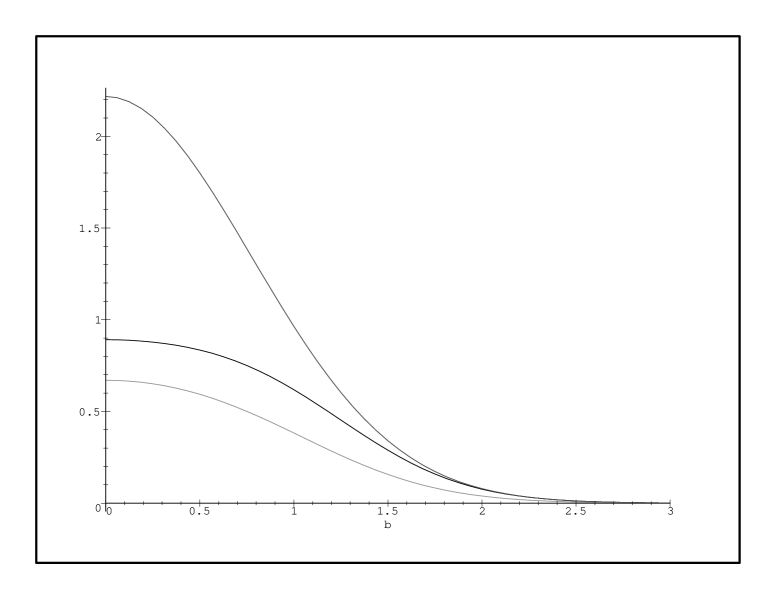
Fig. 33-b

Figure 32: The behaviour of $\Omega(s,b)$ ( dashed curve), $Im\,a_{el}(s,b)$ ( dotted curve) and $G_{in}(s,b)$ ( solid curve) as function of impact parameter $b$( in Fm) at $s=400GeV^{2}$ ( a ) and $s=410^{6}GeV^{2}$ ( b ).

For both energies $\Omega\,>\,1$ which leads to sufficiently big SC in $G_{in}$. However, since the SC in the elastic amplitude depend on $\Omega/2$, they are much smaller. $G_{in}$ is close to 1: in the intermediate energy region the unitarity requirement has a simple solution,   $a_{el}\,\approx\,\frac{1}{2}$ which is obtained $G_{in}=1$ is used in Eq.(20) together with $|a_{el}|^{2}\,\ll\,Im\,a_{el}$.

The lesson is very simple: if we want to measure the SC we have to find a process which depends on $G_{in}$. Certainly, it is not the total cross section nor the elastic one. We can see from Fig.33 that we need a process which is sensitive to small impact parameters, namely, $b\,\leq\,1Fm$.

12.5 Large Rapidity Gap processes and their survival probability.

We call any process a LRG process if over a sufficiently large rapidity region no hadrons are produced. Single and double diffractive dissociation or central diffraction are examples of such processes ( see Fig.24). Bjorken advocated to study LRG processes which have the additional signature of a “hard” processes. The simplest example of such a process is the production of two large transverse momenta jets with LRG between them ( $\Delta y=|y_{1}\,-\,y_{2}|\,\gg\,1$ ) in back - to - back kinematics ( $\vec{p}_{t1}\,\,\sim\,\,-\,\vec{p}_{t2}$ ). Let us consider this reaction in more details to illustrate how Pomeron “soft” physics enters the calculation of such a typical “hard” process. I will discuss such processes in a more detailed form in the third part of my lectures but, I hope, that a brief discussion here will help to understand how important it is to get more reliable knowledge on the SC.

The reaction which we consider is ( see Figs. 23-d and 24 for notations):

$$p\,\,+\,\,p\,\,\rightarrow\,\,$$ (112)

$$M_{1}\,\{\,\,hadrons\,\,+\,\,jet_{1}(\,x^{1},\vec{p}_{t1}\,)\,\}\,\,+\,\,[\,LRG\,(\,\Delta y\,=\,|y_{1}-y_{2}|\,)\,]\,\,+\,\,M_{2}\,\{\,\,hadrons\,\,+\,\,jet_{2}(\,x^{2},\vec{p}_{t2}\,)\,\}\,\,,$$

where

$$x^{1}\,\,=\,\,\frac{2\,p_{t1}}{\sqrt{s}}\,e^{y_{1}}\,\,;$$

$$x^{2}\,\,=\,\,\frac{2\,p_{t2}}{\sqrt{s}}\,e^{y_{2}}\,\,;$$

and

$$\vec{p}_{t1}\,\,\approx\,\,-\,\vec{p}_{t2}\,\,;\,\,\,\,\,\,p_{t1}\,\approx\,p_{t2}\,\,\gg\,\,\mu\,\,.$$

We denote by $\mu$ the typical scale for transverse momentum for “soft” processes.

The cross section of this reaction can be described by a factorization formula:

$$f(\,\Delta y,y_{1}+y_{2},p_{t1},p_{t2}\,)\,\,=\,\,\frac{d\sigma}{d\Delta y,d(y_{1}+y_{2})dp^{2}_{t1}dp^{2}_{t2}}\,\,=$$ (113)

$$F^{(1)}_{p}(x^{1},p^{2}_{t1})\cdot F^{(2)}_{p}(x^{2},p^{2}_{t2})\cdot\sigma_{hard}(p^{2}_{t1},x^{1}x^{2}s)\,\,,$$

where $F^{i}_{p}$ is probability to find a parton with $x^{i}$ in the proton ( deep inelastic structure function) and $\sigma_{hard}$ is the cross section of the “hard” parton - parton interaction at sufficiently large energies ( $x^{1}x^{2}s$ ). We assume, that this “hard” process is due to the exchange of a colourless object which we call “hard” Pomeron which will be discussed in the later parts of my lectures; here we concentrate on the calculation of the probability for such a reaction. Reaction of Eq. (112) can be viewed as a statistical fluctuation of the typical inelastic event. The probability for such a fluctuation is small and is of the order of $exp(-<n(\Delta y)>)$ where $<n(\Delta y)>$ is the average hadron multiplicity of a typical inelastic event in the rapidity region $\Delta y$.

Secondly, we need to multiply Eq. (113) by the so called damping factor $<D^{2}>$ . It gives the probability that no partons with $x>x^{1}$ from one proton and no partons with $x>x^{2}$ from the other proton will interact with each other inelastically. In general, such an interaction produces many hadrons in the rapidity region $\Delta y$, therefore, they must be excluded in the correct expression for the cross section. Let me point out that Eq. (113) is correct if one believes that the exchange of a single Pomeron describes the “soft” processes, an assumption which is made for the D-L Pomeron. Therefore, the experimental deviation from Eq. (113) itself gives a model independent information on whether or not the single Pomeron is doing its job. Remember that we need to calculate $<D^{2}>$. We have discussed that

$$P(s,b)\,\,=\,\,e^{-\,\Omega(s,b)}\,\,$$ (114)

is equal to the probability that no inelastic interaction between the scattered hadron has happened at energy $\sqrt{s}$ and impact parameter $b$. Therefore, in the Eikonal model $P(s,b)$ is just the factor that we need to multiply Eq. (113) to get a right answer:

$$f(\,\Delta y,y_{c}=y_{1}+y_{2},p_{t1},p_{t2}\,)\,\,=\,\,<D^{2}>f(\,{Eq.~{}(\ref{LRGCR})}\,)\,\,,$$ (115)

where

$$<D^{2}>\,\,=\,\,\frac{\int\,d^{2}bP(s,b)\cdot f(b,\Delta y,y_{c},p_{t1},p_{t2}\,)}{\int\,d^{2}bf(b,\Delta y,y_{c},p_{t1},p_{t2}\,)}\,\,.$$ (116)

Here we introduce $f(b,\Delta y)$ using the following formula:

$$f(b,\Delta y)\,\,=\,\,\int d^{2}b^{\prime}d^{2}b"F^{1}_{p}(b^{\prime};x^{1},p^{2}_{t1})\cdot\sigma_{hard}(b^{\prime}-b",x^{1}x^{2}s)\cdot F^{1}_{p}(b-b^{\prime};x^{2},p^{2}_{t2})\,\,,$$ (117)

where

$$F^{i}_{p}(x^{i},p^{2}_{ti})\,\,=\,\,\int d^{2}b^{\prime}F^{1}_{p}(b^{\prime};x^{i},p^{2}_{ti})\,\,.$$

Actually, for the deep inelastic structure function we can prove that the impact parameter behaviour can be factorized out in the form

$$F^{1}_{p}(b^{\prime};x^{1},p^{2}_{t1})\,\,=\,\,S(b)\cdot F^{1}_{p}(x^{1},p^{2}_{t1})\,\,,$$

where $\int d^{2}bS(b)\,=\,1$.

One can also see that the “hard” process is located at a very small value of $b^{\prime}-b"$. Just from the uncertainty principle $b^{\prime}-b"\,\propto\,1/p_{t1}\,\,\ll\,$ any impact parameter scale for “soft” processes. Finally, we can use $b^{\prime}=b"$ in the integral of Eq. (117).

It is now easy to see that the damping factor can be calculated as:

$$<D^{2}>\,\,=\,\,\int d^{2}bd^{2}b^{\prime}\,P(s,b)\cdot S(b^{\prime})\cdot S(b-b^{\prime})\,\,.$$ (118)

For $S(b)$ we use the exponential parameterization,namely

$$S(b)\,\,=\,\,\frac{1}{\pi R^{2}_{H}}\,\,e^{-\,\frac{b^{2}}{R^{2}_{H}}}\,\,.$$ (119)

Taking the integral over $b^{\prime}$ we get

$$<D^{2}>\,\,=\,\,\int db^{2}\,P(s,b)\cdot\frac{1}{2R^{2}_{H}}\,\,e^{-\,\frac{b^{2}}{2\,R^{2}_{H}}}\,\,.$$ (120)

Fortunately, the value of $R^{2}_{H}$ has been measured at HERA and is equal to

$$R^{2}_{H}\,\,=\,\,8\,\,GeV^{-2}\,\,.$$

Of course, $R_{H}$ does not depend on energy. In Fig.34 one sees the impact parameter dependence of

$$\Gamma(s,b)\,\,=\,\,P(s,b)\cdot e^{-\,\frac{b^{2}}{2\,R^{2}_{H}}}\,\,,$$

or, in other words, of the profile function for the LRG process. From this figure one concludes that the damping factor should be rather small since $\Gamma$ turns out to be much smaller than $G_{in}$. Secondly, LRG processes in general have larger impact parameters than the average inelastic process since the $b$ - distribution shows a dip in the region of small $b$ and therefore, almost all LRG processes have $b\,\approx\,1Fm$.

Integration in Eq. (120) gives:

$$<D^{2}>\,\,=\,\,a\,\cdot\,(\frac{1}{\nu(s)})^{a}\,\cdot\,\gamma(a,\nu(s))$$ (121)

where $\gamma(a,\nu)$ is the incomplete Gamma function

$$\gamma(a,\nu)\,=\,\int^{\nu}_{0}\,z^{a-1}\,e^{-z}\,d\,z\,\,$$

and

$$a\,\,=\,\,\frac{R^{2}(s)}{2R^{2}_{H}}\,\,.$$

The energy behaviour of the damping factor is given in Fig.35a. One can see that in this simple model the damping factor is about 30% and drops by about a factor of two from the Fermilab fixed target experiment energies to the Tevatron energies.

It is interesting to note that the single diffraction process which is also a LRG process in the Eikonal model has a similar damping factor. The difference is only in the definition of parameter $a$ or rather in the value of $R_{H}$ which starts to depend on energy. It turns out that for single diffraction

$$a\,\,=\,\,\frac{2R^{2}(s)}{(\,R^{2}(s)\,+\,R^{2}(M^{2})-R^{2}(s=s_{0})\,)}\,\,.$$

In Fig.35b we plot the energy behaviour of the single diffraction cross section in the triple Pomeron formula ( see Eq.(76) ) and after taking into account $<D^{2}>$. One can see that there is a striking difference in the energy behaviour. In my opinion this is direct experimental evidence that the SC must be taken into account in addition to the Pomeron exchange.

Fig.35-a

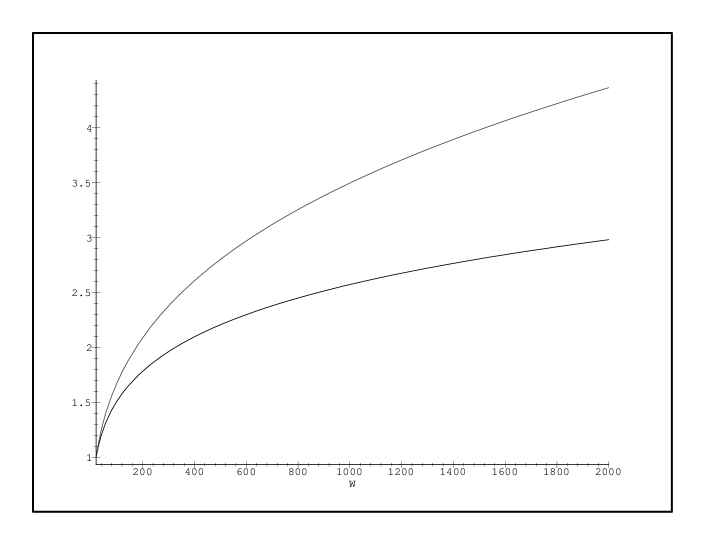
Fig. 35-b

Figure 34: The energy behaviour of the damping factor for the “hard” processes with LRG (Fig. 35a ) and for the cross section of single diffraction dissociation (Fig.35b): for the triple Pomeron formula (dashed line) and for the triple Pomeron formula multiplied by damping factor( solid line ), $W\,\,=\,\,\sqrt{s}$.

12.6 $\sigma_{tot}$,   $\sigma_{el}$ and slope $B$.

Using the general formulae of the Eikonal model( see Eqs.(108) - (110) ) one can easily obtain the expression for the total cross section and for the elastic one after integration over $b$. I hope that you will be able to perform this integration with $\Omega$ given by Eq.(110); the result is:

$$\sigma_{tot}\,\,=\,\,2\,\pi\,R^{2}(s)\,\{\,\,ln(\Omega(s,b=0)/2)\,\,+\,\,C\,\,-\,\,Ei(-\Omega(s,b=0)/2)\,\,\}$$ (122)

and

$$\sigma_{el}\,\,=$$ (123)

$$\pi\,R^{2}(s)\,\{\,ln(-\Omega(s,b=0)/4)\,+\,C\,+\,Ei(\,-\Omega(s,b=0)\,)\,-\,2Ei(\,-\Omega(s,b=0)/2)\,)\,\}\,\,.$$

Here, C= 0.5773 is the Euler constant and $Ei(x)$ denotes the integral exponent $Ei(x)\,=\,\int^{x}_{-\infty}\,\,\frac{e^{-t}}{t}dt$.

In Figs.36a and 36.b we plot the energy dependence of the total and elastic cross sections. One can see that in spite of the fact that the influence of the SC can be seen at high energy it is not as pronounced as in the value of the damping factor and/or in the energy dependence of the diffractive dissociation cross section.

For completeness let me present here the calculations for the slope $B$ which can be defined as

$$B\,\,=\,\,\frac{ln\frac{d\sigma}{dt}}{dt}\,\,|_{t=0}\,\,.$$

Using the impact parameter representation one finds

$$B\,\,=\,\,\frac{\int\,b^{2}\,Im\,a_{el}(s,b)\,d^{2}b}{2\,\int\,Im\,a_{el}(s,b)\,d^{2}b}\,\,.$$ (124)

We can rewrite Eq. (124) as a ratio of two hypergeometrical functions

$$B\,\,=\,\,\frac{R^{2}(s)}{2}\,\cdot\,\frac{hypergeom(\,[1,1,1],[2,2,2],-\Omega(s,b=0)/2\,)}{hypergeom(\,[1,1],[2,2],-\Omega(s,b=0)/2)\,)}\,\,.$$ (125)

Here I used the notation of Maple for the hypergeometrical functions to give you a possibility to check the numerics. The calculations plotted in Fig.36c were done with the same values for the parameters of the Eikonal model as have been discussed before in section 12.4. One can see that the SC induce a larger shrinkage of the diffraction peak ($s$-dependence of the slope $B$ ) than in the simple one Pomeron exchange approach.

The reason why I discussed these typical “soft” processes observables is to show you that the SC manifest themselves differently for different processes, compare e.g. Figs.36 and Figs.35.

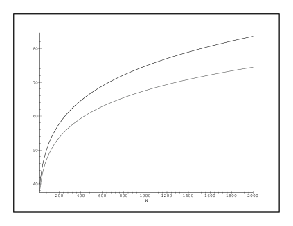
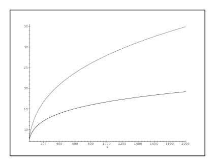
Fig. 36-a	Fig. 36-b
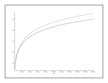
Fig. 36-c

Figure 35: The energy dependence of $\sigma_{tot}$, $\sigma_{el}$ and the slope $B$ of the Eikonal model for the SC ( dashed curves) and for the one Pomeron exchange approach ( solid curves).

12.7 Inclusive production.

12.7.1 Cross section.

We have already discussed the main result for the inclusive cross section: due to the AGK cutting rules all SC cancel and only the Pomeron exchange gives a nonzero contribution ( see Fig.37a ). We want now to stress that according to AGK cutting rules only the SC induced by interaction between a parton with rapidity larger than $y$ with a parton with rapidity smaller that $y$ give a contribution to the inclusive cross section. All interactions between two or more partons with rapidity larger than $y$ are possible as well as interaction of the produced particle with the parton cloud (see Fig.37a). In the framework of the Eikonal model we neglect such interactions and, therefore, only in the Eikonal model we can prove that the simple one Pomeron exchange diagram for the inclusive cross section describes the cross section for inclusive production.

However, even in the general approach the single inclusive cross section has a factorization form and can be written as:

$$\sigma_{inc}(a+b\,\rightarrow\,c+X)\,\,=\,\,a\,\sigma^{(a+c)}_{tot}(s_{1})\,\cdot\,\sigma^{(b+c)}_{tot}(s_{2})\,\,,$$ (126)

where $a$ is constant and $s_{1}\,=\,x_{1}s$ and $s_{2}\,=\,x_{2}s$ with $x_{1}\,=\,\frac{m_{tc}}{\sqrt{s}}\,e^{y_{1}}$ and $x_{2}\,=\,\frac{m_{tc}}{\sqrt{s}}\,e^{-y_{1}}$ ($m_{tc}\,=\,\sqrt{m^{2}_{c}+p^{2}_{tc}}$ ).

In the third part of my lectures I will show that this factorization leads to the factorization theorem for “hard” processes.

12.7.2 Correlations.

We have discussed the two particle rapidity correlation for the inclusive reaction in section 9.8 ( see Fig. 23f ) for one Pomeron exchange. We found that in the correlation function $R$ given by Eq.(82) only the contribution from the first diagram in Fig.37b survives leading to the simple formula of Eq.(83). This equation describes the so called “ short range” rapidity correlations which vanish at large values of $\Delta y=|y_{1}-y_{2}|$ as

$$R\,\,\rightarrow|_{\Delta y\,\gg\,1}\,\,SR\,\cdot\,e^{-\frac{\Delta y}{L_{cor}}}\,\,.$$ (127)

A new contribution comes from the SC and due to the same AGK cutting rules the contributions from all diagrams cancel in the correlation function except one, namely, the two Pomeron exchange shown in Fig.37b. A look at this diagram shows that it does not depend on the rapidity difference ($\Delta y$) and, therefore, gives a constant contribution to the correlation function $R$ which we call long range rapidity correlations. Therefore, the general form for the rapidity correlation function $R$ (see Eq.(82) for the definition) at large $\Delta y$ is

$$R\,\,=\,\,SR\cdot\,e^{-\frac{\Delta y}{L_{cor}}}\,\,+\,\,LR$$ (128)

The constant term $LR$ can be estimated using the AGK cutting rules. The cross section for two particle production from different Pomerons (“ladders” in Fig.32 ) is equal to $\sigma^{(2)}_{2}\,\,=\,\,2\,\Delta\sigma_{tot}$ and $\sigma_{tot}\,=\,\sigma^{P}_{tot}-\Delta\sigma_{tot}$, where $\sigma^{P}_{tot}$ is the total cross section in the one Pomeron exchange model and $\Delta\sigma_{tot}$ is correction to the total cross section due to two Pomeron exchange. Therefore,

$$LR\,\,=\,\,2\frac{\Delta\sigma_{tot}}{\sigma_{tot}}\,\,.$$ (129)

In the Eikonal model one finds $\Delta\sigma_{tot}$, expanding Eq.(108), namely

$$\Delta\sigma_{tot}\,\,=\,\,\frac{\pi}{2}\,\int b^{2}\Omega^{2}(s,b)\,\,$$ (130)

which gives in the parameterization of Eq.(110) for $\Omega$

$$\Delta\sigma_{tot}\,\,=\,\,\frac{\sigma^{2}_{0}(s=s_{0})}{\pi\,4\,R^{2}(s)}\cdot(\,\frac{s}{s_{0}}\,)^{2\,\Delta_{P}}\,\,.$$ (131)

Using Eq. (131) and Eq. (130), we obtain the following estimates for the term $LR$ in Eq. (128):

$$RL\,\,=\,\,\,\frac{\sigma^{2}_{0}(s=s_{0})}{\sigma_{tot}\,\pi\,4\,R^{2}(s)}\cdot(\,\frac{s}{s_{0}}\,)^{2\,\Delta_{P}}\,\,.$$ (132)

In Fig.37c the value of $LR$ term is plotted as a function of energy. For $\sigma_{tot}$ we used Eq.(121). One can see that the long range rapidity correlations are rather essential and give positive correlation of the order of 30% - 50%.

We can also write the two Pomeron contribution to the total double inclusive cross section ( $\sigma^{DP}$ ) in the form:

$$\sigma^{DP}\,\,=\,\,m\,\frac{\frac{d\sigma}{dy_{1}}\,\frac{d\sigma}{dy_{2}}}{2\,\sigma_{eff}}$$ (133)

where $m$ is equal 1 for identical particle $1$ and $2$ while it is equal to 2 if they are different. The Eikonal model predicts for $\sigma_{eff}\,=\,25\,mb$ at $W=\sqrt{s}=20GeV$ rising to $38\,mb$ at the Tevatron energies ( $W=2000GeV$). We will use the form of Eq. (133) in the next section in discussion of the CDF data.

Figure 36-a: Single inclusive cross section with shadowing corrections.

Figure 36-b: Correlation function $R$ (see Eq.(82) ) with shadowing corrections.

Figure 36-c: The value of the long range rapidity correlation term ( $LR$)(see Eq. (128) ) in the Eikonal model.

13 The Pomeron from HERA and Tevatron experiments.

13.1 Reggeon approach strategy for measuring the Pomeron structure.

The question which I am asking: what is the correct strategy to measure the Pomeron structure? I hope, that you are now in a position to answer this question.

Let me give you my answer:

1. We must measure the intercept of the Pomeron as well as which type of inelastic processes proceed Pomeron exchange

(i) in the inclusive processes where the most part of the shadowing corrections mostly cancel

and

(II) in the short range ( in rapidity ) part of the correlation function.

These are the best signatures for one Pomeron exchange.

2. The traditional observables like the total cross section, the elastic cross section and the diffractive dissociation cross sections cannot be recommended for determining the Pomeron structure since they suffer from large contribution from shadowing corrections. Among these three the least informative is the diffractive dissociation cross section, very bad is the elastic one and bad is the total cross section as far as the value of the SC is concerned.

3. The $t$ - dependence of the Pomeron trajectory and of the vertices of interaction with particles and between Pomerons is very interesting since it is closely related to the typical distances involved in the Pomeron problem. Unfortunately, I do not know a way of measuring these other than to measure the traditional observables like the value and the shrinkage of the $t$ - slope of elastic and diffractive cross sections. We have discussed that these are not the best observables but nobody knows better ones.To diminish the influence of the SC we have to measure all slopes at very small values of $t$. I would like to emphasize this point of view since this is the real justification why we need to measure the classical observables at a new generation of accelerators in spite of the fact that it looks old fashioned and not very informative. At the moment this is the only way to find out the scale of distances which are responsible for “soft” interactions.

4. The energy behaviour of the diffractive dissociation in DIS. For large values of the photon virtuality ( $Q^{2}$) the SC tends to be negligible and only one Pomeron exchange contributes to this process. However, the interpretation of this process in terms of Pomeron exchange at large $Q^{2}$ is highly questionable and demands the experimental study of which distances are essential in diffractive processes.

However,  if  I  will  ask   you   what  is   the best    way   to   measure   the shadowing      corrections, the answer will be just the opposite:

1. The best way is the diffractive dissociation processes, worse elastic scattering, very bad is the total cross section and extremely bad is the inclusive one. However, here I want to make a remark on diffractive dissociation in photon - proton interaction. As discussed the photon looks like a collection of hadrons with a broad mass spectrum. This means that when measuring the diffractive cross section in photon - hadron interactions we measure mainly elastic scattering between hadrons of the appropriate masses. Therefore, unfortunately, in photon - hadron interaction we have not found yet the best process. The single photon diffraction dissociation certainly is not the best one.

2. One can improve the situation by measuring double diffractive dissociation. The hadron vertex looks the same as in hadron - hadron collisions and the double diffractive dissociation provides a tool to measure the SC.

3. I am certain that the best way of extracting the SC in photon - hadron interactions and one of the best in hadron - hadron collisions is the long range ( in rapidity ) part of the correlation function. I will show below how this sort of measurement by CDF led to a breakthrough in the issue of the SC.

4. The direct way of measuring the value of the SC are LRG processes especially the “hard” ones. The real measurement of the damping factor, which as it turns out to be rather big will provide unique information on the SC.

And let me ask you the third question: what is the most fundamental problem for the Pomeron?

As I have discussed, the Pomeron hypothesis is the outcome mostly of lack of imagination and we have no real deep argument that the high energy asymptotic should be Pomeron like. However, this hypothesis works well phenomenologically. My answer is that in the framework of the Pomeron hypothesis the fundamental problem is to understand experimentally and theoretically what is going on with diffractive production of large masses. As I have discussed, the main difficulties of the Pomeron approach are concentrated in this problem. Theoretically, solution to this problem means that we understood how the SC work between every possible parton.

13.2 The Pomeron before HERA and Tevatron.

Our knowledge about the Pomeron before HERA and Tevatron can be described as Donnachie - Landshoff Pomeron . Actually, it is not correct to call this Pomeron the D-L Pomeron. Many people introduced such a Pomeron long before D-L ( K.A.Ter-Martirosian, A.Kaidalov et al. in Moscow, A. Capella, Tranh Tran Van et al in Orsay and many others ) but we have to give a credit to Donnachie and Landshoff -  they were the first ones who assumed that there is nothing but the D-L Pomeron. We have discussed the certain theoretical difficulties with the D-L Pomeron, but let us look at the D-L Pomeron from a different angle,namely, as the most ecanomic way to express the experimental data. Let us list the parameters of the D-L Pomeron and let us try to extract physics out of them.

1. $\alpha_{P}(0)\,\,=\,\,1.08$ or $\Delta_{P}\,=\,\alpha_{P}\,-\,1\,=\,0.08$.

This is a small number. What does the smallness mean using the parton model as a guide? Firstly, let me make an essential remark about partons. In QCD partons are gluons ( massless particles with spin one ) and quarks and antiquarks( massive with spin 1/2 ). Going back to Eq.(60) one can see that in the $g\phi^{3}$ model there is an extra power of $s$ in front of the formula for the cross section. Actually, in the general case the power of $s$ is as follows : $(1/s)^{2j-2}$ where $j$ is the spin of partons. It is obvious that in QCD mainly gluons contribute to the expression for the cross section because for them the extra power of $s$ is just equal to zero. In this particular case, the intercept of the Pomeron is equal to $\alpha_{P}(0)\,\,=\,\,\Sigma(0)$ and closely related to the parton multiplicity $(N_{G})$ which is $N_{G}\,\,=\,\,\Sigma(0)\ln(s)$.

Therefore, the smallness of the Pomeron intercept means that the main contribution to the Pomeron structure originate from the first “Born” diagram = the two gluon exchange, but most likely with completely nonperturbative gluons which carry the nonperturbative scale ($\mu$ in the parton model). The production of gluons could be considered in a perturbative way with respect to $\alpha_{P}(0)$.

2. $\alpha^{\prime}_{P}(0)\,\,=\,\,0.25GeV^{-2}$.

Once more a small value ( remember thayt for Reggeons typically $\alpha^{\prime}_{R}\,\approx\,0.7\,-\,1\,GeV^{-2}$ which , at first sight, says that we have a large typical transverse momentum scale in the Pomeron. Let us estimate this using Eq.(60) and expanding $\Sigma(q^{2})$ as a function of $q^{2}$ at small $q^{2}$ which gives

It gives:

$$\alpha_{P}(q^{2})\,\,=\,\,\Sigma(0)\,\,-\,\,q^{2}\frac{\Sigma(0)}{6\mu^{2}}\,\,.$$ (134)

Comparing Eq. (134) with the value for $\alpha^{\prime}_{P}(0)$ we find that $\mu\,\approx\,250MeV\,\approx\,\Lambda$, where $\Lambda$ is the QCD scale parameter.

3. The experimental slope for the $t$-dependence of the triple Pomeron vertex ($r^{2}_{0}$) turned out to be smaller than the slope of the Pomeron proton form factor ( $R^{2}_{0}$ ): $r^{2}_{0}\,\,\leq\,1\,GeV^{-2}\,\,\ll\,\,R^{2}_{0}\,\,=2.6\,GeV^{-2}$ in all so-called triple Reggeon fits of diffractive dissociation data. Unfortunately, the accuracy of the data was not so good and the value of $r^{2}_{0}$ could not be defined by the fit. Actually, the fit could be done with $r^{2}_{0}=0$. This observable is very important since it gives a direct information on the transverse momentum scale is responsible for the Pomeron structure. As we have seen the value of $\alpha^{\prime}_{P}(0)$ depends on the unknown parton density while $r^{2}_{0}$ does not.

4. The ideas of the additive quark model that a hadron has two scales, namely, the hadron size $R\,\approx\,1\,fm$ and the size of the constituent quark $r_{Q}\,\approx\,0.2-0.4\,fm$; is still a working hypothesis and it was included in the D-L Pomeron to the $t$ - dependence of the Pomeron - hadron vertices.

5. Regge factorization has been checked and it works, but the number of reactions studied was limited.

13.3 Pomeron at the Tevatron.

The Tevatron data as well as the CERN data especially on diffractive dissociation, I think, contributed a lot to our understanding of the Pomeron structure. It is a pity that this contribution has not been properly discussed yet. Let me tell you what I learned from the Tevatron.

1. The measurement of the inclusive cross section at Tevatron energy allowed us to extract the intercept of the Pomeron from the energies behaviour of the inclusive spectra in the central rapidity region. The result was surprising: the energy behaviour of the inclusive cross section can be parameterized (Likhoded et al. 1989) as

$$C_{0}\,+\,C_{P}(s/s_{0})^{\Delta_{P}(0)}\,\,,$$ (135)

with $\Delta_{P}(0)\,=\,0.2$ instead of the D-L value $\Delta\,=\,0.08$ !!!. Both $C_{0}$ and $C_{P}$ are constant in the above parameterization. In the framework of the Reggeon approach I have to insist that the Pomeron intercept has been measured correctly only in the inclusive cross section and to face the problem that the D-L Pomeron is not a Pomeron at all. Irritating feature of Eq. (135) is the fact that one has to include an additional constant $C_{0}$. Does this mean that I have to deal with two Pomerons: the first with $\Delta_{P_{1}}(0)=0$ ( term $C_{0}$ in Eq. (135) ) and the second with $\Delta_{P_{2}}\,=\,0.2$ ?!

2. The beautiful data on diffractive dissociation which are shown in Fig.26 changed the whole issue of the SC from theoretical guess to a practical nessecity. I have discussed that the Eikonal model for t SC could describe the main feature of the data but I an very certain that data are much richer and have not been absorbed and properly discussed by the high energy community. You can will find some discussions in papers and talks of Gotsman et all (1992), Goulianos (1993 - present), Capella et al. (1997) , C-I Tan (1997), Schlein at al. (1997) and others.

3. The CDF data for the double parton cross section. CDF used the double inclusive cross section to measure the contribution of the SC. Actually, CDF measured the process of inclusive production of two pairs of “hard” jets with almost compensating transverse momenta in each pair and with almost same values of rapidities. The production of two such pairs is highly supressed in the one Pomeron model ( one parton cascade ) and can be produced only via double Pomeron interaction ( double parton collisions). The Mueller diagram for such a process is given in Fig. 38b. We can use formula (132) for this cross section which predicts for $\sigma_{eff}$ in Eq.(132) 14.5  $\pm$ 1.7 $\pm$ 2.3 mb. This value is approximately half as big as our estimates in the Eikonal model. Therefore, these data show that the SC exist and they are even bigger than the Eikonal model estimates. Perhaps, the problem is not in the Eikonal model but in our picture for the hadron which was included in the Eikonal model. Namely, if we try to explore the two radii picture of the proton as it is shown in Fig.38b we will get an average radius which is a factor of two smaller than what has been used. So for me the CDF data finished the discussion of the one Pomeron model, measured the value of the SC and provided a strong argument in favour of the two radii structure of the proton.

Figure 37-a: The J/$\Psi$ production without (a) and with (b) proton dissociation.

Figure 37-b: Inclusive production of two pair of “hard” jets in the double parton scattering.

Figure 37-c: Democratic and two radii picture of proton.

Figure 37-d: Scattering in the constituent quark model.

Figure 37-e: The growth of the interaction radius and the new regime at the LHC energies.

13.4 Pomeron at HERA.

1. I think that HERA did a great thing, namely, the HERA data show explicitly that the hadron has two “soft” scales or two radii. This comes out from the HERA data on photoproduction of the J/$\Psi$ meson. These data show two different slopes in $t$-dependence for quasi-elastic photoproduction and for inelastic photoproduction in which the proton dissociates into a hadron system ( see Fig.38a ): $B_{el}\,\,=\,\,4\,GeV^{-2}$ and $B_{in}\,\,=\,\,1.66\,GeV^{-2}$, while the cross sections are about equal for these two processes. Since in a such a process we can neglect the $t$-dependence of the upper vertex we can interprete these data as follows:

1). as the first measurement of the radius of the so-called Pomeron - proton vertex ( we also called this value the two gluon form factor in a picture of “hard” processes). It turns out that this radius is smaller than the radius given by the electro-magnetic form factor of the proton which for this vertex follows from the additive quark model and has been used for the D-L Pomeron.

2). the second radius which appears can be easily interpreted in the picture of the additive quark model (see Fig.38a) as the proper radius of the constituent quark.

Therefore, HERA finished with a democratic picture for gluons and valence quarks and proved the two radii picture of the proton (see Fig. 38c), which could be an additive quark model. The direct observation of the second scale in the “soft” interaction will lead to reconsideration of the simple partonic estimates ( see Eq. (133) ) of the value of $\alpha^{\prime}_{P}(0)$. Our conclusion that the typical scale in the Pomeron problem is about $\Lambda$ QCD should be revised, but this is a certain problem for the future.

2. The measurement for the energy behaviour of the diffractive dissociation process leads to the intercept of the Pomeron $\Delta_{P}(0)\,\approx\,0.2$. As I have mention there could be different interpretation of the experimental data , but in the framework of the Pomeron approach this is the intercept.

3. The HERA data on the deep inelastic structure function $F_{2}$ can be described by the DGLAP evolution equation if we assume an initial parton distribution at $Q^{2}\,=\,Q^{2}_{0}\,=\,3-5GeV^{2}$ with the energy behaviour $F_{2}(x,Q^{2}_{0})\,\propto\,(1/x)^{0.2}$ which corresponds to a Pomeron intercept $\Delta_{P}(0)\,=\,0.2$.

4. Inclusive hadron production by real and virtual photon scattering can be described assuming a Pomeron with the intercept $\Delta_{P}(0)\,=\,0.2$.

Therefore, let me conclude this section with the following statement:

In October 1997 following the HERA and Tevatron data we have :

$\bullet$ The Pomeron intercept $\Delta_{P}(0)\,=\,0.2$;

$\bullet$ The SC are large and approximately twice as big as the Eikonal model estimates;

$\bullet$ The two radii picture of the proton has been proven experimentally and the values of these two radii have been measured.

14 Instead of conclusions.

14.1 My picture for the high energy interaction.

Let me conclude my lectures sharing with you the truth that as starting from the year 1977 I do not believe in the Pomeron as a specific Regge pole. In the framework of these lectures I could not show you why and it will be a subject for the second part. Instead of the Pomeron approach Ryskin and me developed a different approach which corresponds to the following simple picture (see Figs.38c and 38d) with two ingredients: the constituent quark model for hadrons and the ”black” disc interaction between two constituent quarks. Now, finally, I have the real pleasure telling you that due to the results of HERA we have an experimental confirmation of this approach. Indeed, let us estimate the value of the total cross section for quark - quark interactions. As we have discussed in section 2.4 the cross section is equal to

$$\sigma_{tot}(q+q)\,\,=\,\,2\,\pi(2\,\,r^{2}_{Q})\,\,$$

where $r_{Q}$ is the quark radius, the factor 2 emerges because two quarks collide. Substituting $2r^{2}_{Q}\,=\,B_{in}$ ( see Fig.38a ) we get $\sigma_{tot}(q+q)\,=\,4\,-\,5\,mb$ which gives the correct order of magnitude value for the total proton - proton cross section $\sigma_{tot}(p+p)\,=\,9\,\sigma_{tot}(q+q)$.

In this model the size of the constituent quarks increases with energy (see Fig. 38e) and only at LHC energies the clouds of partons from different constituent quarks will start to overlap. This is the region where we can expect to see new physics for “soft” processes.

The interesting feature of this model is that a substantial part of Regge factorization relations holds because of the simple fact that only quarks interact.

14.2 Apology and Acknowledgements.

Reading back my lectures I found that I have kept my promise and have shared with you all ideas, hopes and difficulties of the Pomeron problem. I hope that after reading these lectures you will know enough about Pomerons to support or to reject this approach.

I thought that I would not give references in this part but one short story changed my mind. Once, when actually I have finished my writing, Aharon Levy called me asking for a help. He tried to find the book of Collins on Regge theory. Indeed, it is the last book on the subject which summarizes our knowledge of Reggeon theory. However, he failed to find it in any library in Hamburg, DESY one including. I also could not find but fortunately, I went to Paris and found one copy in the LPTHE at Orsay. I asked the librarian to check whether the general library has this book. It turnes out that no and even more no university libraries in Paris have. So, my usual excuse that you could easily find everything that I have discussed in any book of the sixties being correct is not practical. So, I decided to give a list of references which is far from being full but at least you will be able to read and clarify a subject that you feel to be interesting. By the way, the end of the story with Collins book is happy. In December, Aharon Levy (tel. 2001 at DESY ) will be the only one who will have the copy of the book.

I wish to express my deep apology to all my friends whom I did not cite. I hope to prepare the full list of references including Russian physicists to conclude the last part of my lectures.

As I have mentioned I have learned everything about the Pomeron from Prof. Gribov and I was actively involved in this problem during the best fifteen years of my life in the Leningrad Nuclear Physics Institute under the leadership and strong influence of Prof. Gribov. I cannot express, at least in english, my deep sorry that we lost him. These lectures are an attempt to look at the problem with his eyes and, unfortunately, this is the only thing I can do now for him.

I am very grateful to my friends A. Kaidalov, O. Kancheli and M. Ryskin for a life long discussions of the Pomeron. I am sure that a lot of ideas, that we discussed, have shown up in these lectures. I thank E.Gotsman and U.Maor who started with me five years ago an attempt to revise the whole issue of the Pomeron approach. Sections, devoted to the Eikonal model, is written on the basis of our common papers as well as our common understanding that the Donnachie - Landshoff Pomeron is not the right one. E. Gotsman calculated Fig.25 which I used here and I thank him for this. Travelling around the globe I met the Old Reggeon Guard: J. Bartels, K. Boreskov, A. Capella, J.Cohen - Tannoudji,P. Collins, A.Donnachie, A. Krzywicki,S. Matinian, A. Mueller, R. Peschanski, A. Santoro, C-I Tan, K.A. Ter - Martirosian and A. White ( more names for search). Most of them, as well as me, are doing quite different things but all of them still keep alive the interest for the beauty of this difficult problem. My special thanks to them for encouraging optimism.

These lectures would be impossible without help and support of my DESY friends W. Buchmueller, J. Dainton, H. Kowalski and G. Wolf. I am grateful to them as well as to my listerners who asked many good questions which have improved the presentation and contents. Hope for more questions and critisism.

15 References.

Books:

1. G.F. Chew: “ S- matrix theory of strong interaction”, Benjamin, 1962.

2. S.C. Frautschi:“ Regge Poles and S-matrix Theory”, Benjamin, 1963.

3. R. Omnes and M. Froissart: “Mandelstam Theory and Regge Poles: An Introduction for Experimentalists”, Benjamin, 1963.

4. M. Jacob and G.F.Chew:“Strong interaction physics”, Frontiers in Physics, 1964.

5. R.J. Eden, P.V. Landshoff, D.I. Olive and J.C. Polkinghorne: “ The analytic S - matrix”, Cambridge U.P., 1966.

6. R.J. Eden: “ High energy collisions of elementary particles”, Cambridge U.P. 1967.

7. V. Barger and D. Cline: “ Phenomenological Theories of High Energy Scattering: An Experimental Evaluation”, Frontiers in Physics, 1967.

8. P.D.B. Collins and E.J. Squires:“ Regge Poles in Particle Physics”, Springer, 1968.

9. A. Martin: “ Scattering Theory: Unitarity, Analyticity and Crossing”, Lecture notes in Physics, Springer, 1969.

10. R. Omnes: “ Introduction to particle physics”, Wiley, 1971.

11. R. Feynman: “ Photon - hadron interaction ”, Benjamin, 1972.

12. D. Horn and F. Zachariasen: “ Hadron Physics at Very High Energies”, Benjamin, 1973.

13. S.J. Lindenbaum: “ Particle Interaction Physics at High Energy”, Clarendon Press, 1973.

14. M. Perl: “ High energy hadron physics”, Wiley, 1974.

15. S. Humble: “ Introduction to particle production in hadron physics”, Academic Press, 1974.

16. “Phenomenology of particles at high energy”, eds. R.L. Crawford and R. Jennings, Academic Press, 1974.

17. P.D.B. Collins: “An introduction to Regge theory and High energy physics”, Cambridge U.P., 1977.

18. Yu. P. Nikitin and I.L. Rosental: “ Theory of Multiparticle Production Processes”, Harwood Academic, 1988.

19. “Hadronic Multiparticle Production”, ed. P. Carruther, WS, 1988.

20. J.R. Forshaw and D.A. Ross: “ QCD and the Pomeron”, Cambridge U.P. 1997.

21. The collection of the best original papers on Reggeon approach: “ Regge Theory of low $p_{t}$ Hadronic Interaction”, ed. L. Caneschi, North - Holland, 1989.

Reviews:

1. P.D.B. Collins: “ Regge theory and particle physics”, Phys. Rep.1C (1970) 105.

2. P. Zachariasen: “ Theoretical models of diffraction scattering”, Phys. Rep. 2C (1971) 1.

3. D. Horn: “ Many particle production”, Phys. Rep. 4C (1971) 1.

4. F. J. Gilman: “ Photoproduction and electroproduction”, Phys. Rep. 4C (1971) 95.

5. P.V. Landshoff and J.C. Polkinghorne: “ Models for hadronic and leptonic processes at high energy”, Phys. Rep. 5C (1972) 1.

6. S.M. Roy: “ High energy theorems for strong interactions and their comparison with experimental data”, Phys. Rep. 5C (1972) 125.

7. J. Kogut and L. Susskind: “ The parton picture of elementary particles”, Phys. Rep. 8C (1973) 75.

8. J. H. Schwarz: “ Dual resonance theory”, Phys. Rep. 8C (1973) 269.

9. G. Veneziano: “ An introduction to dual models of strong interaction and their physical motivation”, Phys. Rep. 9C (1973) 199.

10. R. Slansky: “ High energy hadron production and inclusive reactions ”, Phys. Rep. 11C (1974) 99.

11. S. Mandelstam: “ Dual - resonance models”, Phys. Rep. 13C (1974) 259.

12. R.C. Brower, C.E. De Tar and J.H. Wers: “ Regge theory for multiparticle amplitude”, Phys. Rep. 14C (1974) 257.

13. Ya.I. Azimov, E.M. Levin, M.G. Ryskin and V.A. Khoze: “ What is interesting about the region of small momentum transfers at high energies ?”,   CERN-TRANS 74-8, Dec 1974. 196pp. Translated from the Proceedings of 9th Winter School of Leningrad Nuclear Physics Inst. on Nuclear and Elementary Particle Physics, Feb 15-26, 1974. Leningrad, Akademiya Nauk SSSR, 1974, pp. 5-161(translation).

14. I.M. Dremin and A.N. Dunaevskii: “The multiperipheral cluster theory and its comparison with experiment”, Phys. Rep. 18C (1975) 159.

15. H.D.I. Abarbanel, J.D. Bronzan, R.L. Sugar and A.K. White: “ Reggeon field theory formulation and use”, Phys. Rep. 21C (1975) 119.

16. G. Giacomelli: “ Total cross sections and elastic scattering at high energy”, Phys. Rep. 23C (1976) 123.

17. M. Baker and K. Ter Martirosyan: “ Gribov’s Reggeon Calculus”, Phys. Rep. 28C (1976) 1.

18. A.C. Irving and R.P. Worden: “ Regge phenomenology”, Phys. Rep. 36C (1977) 117.

19. M. Moshe: “ Recent developments in Reggeon field theory”, Phys. Rep. 37C (1978) 255.

20. A.B. Kaidalov: “ Diffractive production mechanisms”, Phys. Rep. 50C (1979) 157.

21. S.N. Ganguli andd D.P. Roy: “ Regge phenomenology in inclusive reactions”, Phys. Rep. 67C (1980) 257.

22. K. Goulianos: “ Diffraction interactions of hadron at high energy”, Phys. Rep. 101C (1983) 169.

23. M. Kamran: “ A review of elastic hadronic scattering at high energy and small momentum transfer”, Phys. Rep. 108C (1984) 275.

24. E.M. Levin and M.G. Ryskin: “The increase in the total cross sections for hadronic interactions with increasing energy” Sov.Phys. Usp. 32 (1989) 479.

25. E.M. Levin and M.G. Ryskin: “ High - energy hadron collisions in QCD” Phys. Rep. 189C (1990) 267.

26. A. Capella, U. Sukhatme, C-I Tan and J. Tran Thanh Van: “ Dual parton model”, Phys. Rep. 236C (1994) 225.

27. E. Levin: “The Pomeron: yesterday, today and tomorrow”, hep-ph/9503399 , Lectures given at 3rd Gleb Wataghin School on High Energy Phenomenology, Campinas, Brazil, 11-16 Jul 1994.

28. J. Stirling: “ The return of the Pomeron” Phys.World 7 (1994) 30.

29. A.B. Kaidalov: “ Low - x physics”, Survey in High Energy Physics,9 (1996) 143.