Coupled Channel Analysis of S-Wave ${\pi}{\pi}$ and $K\overline{K}$ Photoproduction

Abstract

We present a coupled channel partial wave analysis of nondiffractive $S-$wave $\pi^{+}\pi^{-}$ and $K^{+}K^{-}$ photoproduction focusing on the $K\overline{K}$ threshold. Final state interactions are included. We calculate total cross sections, angular and effective mass distributions in both $\pi\pi$ and $K\overline{K}$ channels. Our results indicate that these processes are experimentally measurable and valuable information on the $f_{0}$(980) resonance structure can be obtained.

1 Introduction

Photoproduction of $K^{+}K^{-}$ pairs near threshold was previously measured at Daresbury [1] and Hamburg [2]. An interesting result from these experiments was an observation of an asymmetry in the $K^{+}K^{-}$ angular distribution in the invariant mass region close to the threshold. This could be described as an interference of the dominant $P$-wave from the decay of the $\phi(1020)$ meson and an $S$-wave from the decay of the $f_{0}(980)$ resonance. Furthermore, the data [3, 4, 5] agree with the diffractive $\phi$ meson production mechanism. The $f_{0}$ meson is most likely produced nondiffractively since it has different quantum numbers from the photon.

The scalar meson sector of the hadron spectroscopy is still very poorly known. There exist a variety of theoretical models dealing with the structure of scalar mesons. Even in the ordinary quark model a unique $q\overline{q}$ assignment of the scalar ${}^{3}P_{0}$ meson nonet seems to be impossible [6]. This is expected since glueballs can mix with the scalars [7, 8] and naturally lead to a complicated internal structure. Among the scalar mesons isoscalar $f_{0}(980)$ and its isovector partner $a_{0}(980)$ are particularly interesting [9, 10]. The $f_{0}(980)$ branching ratio to $K\overline{K}$ amounts to 22$\%$ which is astonishingly large considering that its mass is below the $K\overline{K}$ threshold as most experimental data suggest. Therefore theoretical models have been formulated in which the $f_{0}(980)$ is a quasibound state of the $K\overline{K}$ pair [11].

One may assume that the $K\overline{K}$ pair can be bound in a similar way as the nuclear forces bind the simplest nucleus – deuteron. There is, however, an important difference between the deuteron and the $K\overline{K}$ quasibound state, namely the $K\overline{K}$ quasibound state can annihilate into a system of two pions ($\pi^{+}\pi^{-}$ or $\pi^{0}\pi^{0}$). Models for a coupled channel pion–pion and kaon–kaon scattering like the one in Ref.[12], have allowed us to obtain some characteristics of the $f_{0}(980)$ meson such as its binding energy, decay width, root mean square radius, branching ratios and various threshold parameters [13]. Calculations of the scalar meson properties have been based, however, on the experimental data which are highly imprecise and even controversial, particularly for the $K\overline{K}$ production near threshold [12]. This is very unsatisfactory if one attempts to fix the theoretical parameters by a comparison with experiment. This situation may be improved in the near future with new data on $f_{0}(980)$ photo- and electroproduction experiments from TJNAF[14]. This goal can be accomplished if a very good effective mass resolution near the $K\overline{K}$ threshold is achieved and a partial wave analysis is performed in different final state channels.

With this background, it is clear that much more extensive and systematic investigations must be performed on the theoretical side. Thus, in this paper, we present a coupled channel $S$-wave analysis of nondiffractive $\pi^{+}\pi^{-}$ and $K^{+}K^{-}$ photoproduction. The internal structure of the scalar meson $f_{0}(980)$ can be studied via the final state interactions of the produced pion or kaon pairs. We expect channel coupling effects to be very important since the final state interaction (FSI) of two pions (kaons) can lead to a production of two kaons (pions) in the resonant $S$–wave[12]. A similar dependence on channel coupling can be seen in $a_{0}(980)$ production leading to a formation of the kaon pairs from the initial $\eta$–$\pi$ system [15], however, the isovector channel will not be discussed in this paper.

At low photon energies the $S$–channel photon–nucleon resonances are expected to give a substantial contribution to the production amplitude. In Ref.[16] Gómez Tejedor and Oset made a comprehensive analysis of $\gamma p\rightarrow\pi^{+}\pi^{-}p$ including contributions from $\Delta(1232),N^{*}(1440)$ and $N^{*}(1520)$ resonances. The model reproduced experimental cross sections fairly well below $E_{\gamma}=800$ MeV and invariant-mass distributions at even slightly higher energies. In the analysis of forward $\pi^{+}\pi^{-}$ and $K^{+}K^{-}$ photoproduction at much higher energies ($E_{\gamma}\stackrel{{\scriptstyle>}}{{\sim}}4\;$ GeV) we expect however that mostly the $t$–channel $\rho$ and $\omega$ meson exchanges become important. This assumption follows from Regge phenomenology where high energy amplitudes are dominated by $t$-channel meson exchange. In this paper, we focus on the coupled channel $S$-wave analysis of forward $\pi^{+}\pi^{-}$ and $K^{+}K^{-}$ photoproduction near the $K{\overline{K}}$ threshold and thus we limit the calculation of the nonresonant two meson production amplitudes to a few Feynman diagrams, schematically shown in Fig. 1.

The paper is organized as follows. In the next section we calculate the amplitude corresponding to the Feynman diagrams of Fig. 1 and show how they are related to the differential cross section in the Born approximation. We also give the partial $S$-wave decomposition of the invariant amplitudes for $\pi^{+}\pi^{-},\pi^{0}\pi^{0}$ and $K^{+}K^{-}$ production. In section III we make an off–shell extension of the Born amplitudes and relate them to the photoproduction potential. The full amplitudes including the channel coupling and final state interactions are also discussed in section III. In section IV numerical results are presented and parameter dependence is addressed. The conclusions and discussions follow in section V.

In the Appendices we summarize the effective interaction Lagrangian used in this analysis (Appendix A), the detailed factors in the current defined in section II (Appendix B) and the results of the $S$-wave amplitude (Appendix C).

2 Nonresonant Two Meson Production Amplitude and Differential Cross Section

As discussed in the introduction, we focus on the coupled channel $S$-wave analysis of nondiffractive $\pi^{+}\pi^{-}$ and $K^{+}K^{-}$ photoproduction near and above the $K{\overline{K}}$ threshold of the ${f_{0}}(980)$ meson. According to the Regge phenomenology, we expect that only the $t$-channel meson exchanges, especially $\rho$ and $\omega$ mesons, are important in the analysis of the $S$-wave forward $\pi^{+}\pi^{-}$ and $K^{+}K^{-}$ photoproduction at higher energies. However, the pion coupling to proton cannot contribute because our calculations are limited only to the $S$-wave final states. As illustrated in Fig. 1, we calculate five diagrams for the $\pi^{+}\pi^{-}$ production and six diagrams for the $K^{+}K^{-}$ production. Among the five diagrams for the $\pi^{+}\pi^{-}$ production, three diagrams correspond to $a=\pi^{\pm}$ and $b=\rho^{0}$ including a contact diagram as required by current conservation. In the remaining two diagrams $a=\rho^{\pm}$ and $b=\omega$. Later, we will refer to the first three diagrams, including the contact term, as the type $I$ and to these with double vector meson exchanges in the t-channel as the type $II$. For the six diagrams of $K^{+}K^{-}$ production, three of them correspond to $a=K^{\pm}$ and $b=\rho^{0}$ (type $I$) and the other three to $a=K^{\pm}$ and $b=\omega$ (again type $I$).

Using the effective interaction Lagrangians listed in the Appendix A, we first define the on-shell meson pair ($\pi\pi$ or $K{\bar{K}}$) production amplitude through the appropriate Born terms. Similar effective hadronic field theories have been extensively used in the single kaon electro- and photoproduction processes [17]. For example, for the double pion photoproduction i.e. $\gamma p\to\pi\pi p$, we have

$$-i(2\pi)^{4}\delta(p^{\prime}+k_{1}+k_{2}-p-q)V_{\pi^{i}\pi^{j}}(k_{1},k_{2},p^{\prime},p,q,s^{\prime},s,\lambda)$$

$$=\langle\pi^{i}(k_{1})\pi^{j}(k_{2})\{p^{\prime}\}|Te^{i\int dx{\cal L}}|\{p\},\{\gamma\}\rangle,$$ (1)

where $i,j=\pm,0$ refer to pion charge, $\{\gamma\}=(q,\lambda)$ is the set of quantum numbers representing the incoming photon momentum and spin projection. The initial and final proton states are parameterized by $\{p\}=(p,s)$ and $\{p^{\prime}\}=(p^{\prime},s^{\prime})$, respectively. For $\gamma p\to\pi^{+}\pi^{-}p$ the expansion of the evolution operator with the Lagrangian ${\cal L}$ given in the Appendix A yields five diagrams with the $t$-channel exchange as mentioned above, i.e. three diagrams with $a=\pi^{\pm}$ and $b=\rho^{0}$ (type $I$) and two diagrams with $a=\rho^{\pm}$ and $b=\omega$ (type $II$) in Fig. 1. Similarly, by expanding the evolution operator in Eq.(1) for $\gamma p\to\pi^{0}\pi^{0}p$ we only obtain two type-$II$ processes with $(a,b)=(\rho^{0},\omega)$ and $(a,b)=(\omega,\rho^{0})$. For the $K^{+}K^{-}$ photoproduction, the expansion of the evolution operator in Eq.(1) generates six diagrams, all of which belong to the type $I$ as we have discussed earlier,i.e. three diagrams with $(a,b)=(K^{\pm},\rho^{0})$ plus three diagrams with $(a,b)=(K^{\pm},\omega)$.

Now, using the notations $m$ and ${\bar{m}}$ for the two produced mesons the total amplitude can be written as

$$V_{m\bar{m}}=\sum_{r=I,II}\bar{u}(p^{\prime},s^{\prime})J_{r,m\bar{m}}\cdot\epsilon(q,\lambda)u(p,s),$$ (2)

where $r=I$ refers to sum over the three diagrams including the contact diagram and $r=II$ denotes the sum over only the two diagrams without the contact diagram as discussed earlier. There are three cases of meson pair photoproduction in this analysis, $m\,\overline{m}$ $={\pi^{+}\pi^{-}},{\pi^{0}\pi^{0}},{K^{+}K^{-}}$. The summary of calculated diagrams for each case of $m\,\overline{m}$ is listed in Table 1. The main part of $V_{m\bar{m}}$ is of course the hadronic current $J_{r,m\bar{m}}^{\mu}$ multiplied by the photon polarization four–vector $\varepsilon(q,\lambda)$. The initial and final proton spinors are denoted by $u(p,s)$ and $\bar{u}(p^{\prime},s^{\prime})$. Calculated expressions for $J_{r,m\bar{m}}^{\mu}$ are given by

$$J_{r,m\bar{m}}^{\mu}=(\alpha_{r,m\bar{m}}g^{\mu\nu}+k_{1}^{\mu}\beta_{1r,m\bar{m}}^{\nu}+k_{2}^{\mu}\beta_{2r,m\bar{m}}^{\nu})\{d_{r,m\bar{m}}\gamma_{\nu}+e_{r,m\bar{m}}(p+p^{\prime})_{\nu}\},$$ (3)

where the variables $\alpha_{r,m\bar{m}},\beta_{1r,m\bar{m}},\beta_{2r,m\bar{m}},d_{r,m\bar{m}}$ and $e_{r,m\bar{m}}$ are written in the Appendix B. Here, $g^{\mu\nu}$ is the metric tensor ($g^{00}=1,g^{11}=g^{22}=g^{33}=-1$) and $\gamma^{\nu}$ are Dirac matrices. The Born double differential cross section is then given by

$$\frac{d\sigma}{dtdM_{m\bar{m}}}={1\over{(2\pi)^{3}}}{{|\vec{\kappa}|}\over{32m_{p}^{2}\omega^{2}}}\sum_{l,l_{z}}\langle|V^{l,l_{z}}_{m\bar{m}}|^{2}\rangle,$$ (4)

where $V_{m\bar{m}}^{l,l_{z}}$ is the partial-wave projected amplitude for the process $\gamma p\rightarrow m\bar{m}p$,

$$V^{l,l_{z}}_{m\bar{m}}=\int d\Omega_{m\bar{m}}Y_{ll_{z}}(\Omega_{m\bar{m}})V_{m\bar{m}}.$$ (5)

Here $l$ is the angular momentum of the relative $m\,\overline{m}$ motion, $l_{z}$ is its projection, $t=(p^{\prime}-p)^{2}$ is the four–momentum transfer squared and $M_{m\bar{m}}=\sqrt{(k_{1}+k_{2})^{2}}$ is the two–meson effective mass. In Eqs. (4) and (5) $|\vec{\kappa}|=\sqrt{M^{2}_{m\bar{m}}/4-m_{m}^{2}}$ and $\Omega_{m\bar{m}}$ is the angle between the relative momentum of the two mesons in their c.m. frame and the direction of the final proton momentum. The photon energy in the laboratory frame is denoted by $\omega$ and $m_{p}$ is the proton mass.

The spin averaged amplitude square in Eq.(4) is given by

$$\langle|V^{ll_{z}}_{m\bar{m}}|^{2}\rangle=\frac{1}{4}\sum_{s,s^{\prime},\lambda}|\langle s^{\prime}|V^{ll_{z}}_{m\bar{m}}|s,\lambda\rangle|^{2}.$$ (6)

Furthermore, because only terms inside the round bracket in Eq.(3) depend on meson momenta, the partial-wave projected Born amplitude can also be written as

$$V^{ll_{z}}_{m\bar{m}}=\sum_{r}\bar{u}(p^{\prime},s^{\prime})J^{ll_{z}}_{r,m\bar{m}}\cdot\epsilon(q,\lambda)u(p,s),$$ (7)

where

$$J^{ll_{z},\mu}_{r,m\bar{m}}=P^{ll_{z},\mu\nu}_{r,m\bar{m}}\{d_{r,m\bar{m}}\gamma_{\nu}+e_{r,m\bar{m}}(p+p^{\prime})_{\nu}\},$$ (8)

and the tensor $P$ is given by

$$P^{ll_{z},\mu\nu}_{r,m\bar{m}}=\int d\Omega_{m\bar{m}}Y_{llz}^{*}(\Omega_{m\bar{m}})(\alpha_{r,m\bar{m}}g^{\mu\nu}+k_{1}^{\mu}\beta_{1r,m\bar{m}}^{\nu}+k_{2}^{\mu}\beta_{2r,m\bar{m}}^{\nu}).$$ (9)

The $S$-wave results of the integration over the solid angle in Eq.(9) are summarized in the Appendix C.

3 Final State Interactions

We now discuss the inclusion of final state interactions (FSI) to the $S$-wave projected amplitudes $l,l_{z}=0,0$. Since we are only interested in the $S$-wave projection we shall drop the partial wave labels $l,l_{z}$ from now on. We also limit the study to $\pi^{+}\pi^{-},\pi^{0}\pi^{0}$ and $K^{+}K^{-}$ coupled channel interactions in the final state.

The full photoproduction amplitude including final state interactions can be written in the operator form as

$${\hat{T}}={\hat{V}}+{\hat{t}}\hat{G}{\hat{V}},$$ (10)

where ${\hat{V}}$ is the photoproduction potential, $\hat{t}$ is the strong FSI t-matrix, and $\hat{G}$ is the propagator of the intermediate state. The matrix elements of $\hat{V}$ are obtained through an off-shell extension of the Born amplitude. This is done by following Ref. [18] and generalizing the relativistic scattering problem to inelastic channels. The final result is the potential $\hat{V}$ obtained as the off-energy-shell extension of the Born amplitudes evaluated in the total c.m. frame. This photoproduction potential is then coupled to FSI t-matrix in the two meson rest frame. For the $\gamma p\to m\bar{m}p$ photoproduction the matrix element of Eq. (10) is given by

$$T_{m\bar{m}} = \langle m\bar{m},\vec{\kappa},\{p^{\prime}\}|\hat{T}|\{p\},\{q\}\rangle$$ (11)

$$= \langle m\bar{m},\vec{\kappa},\{p^{\prime}\}|\hat{V}|\{p\},\{q\}\rangle$$

$$+ 4\pi\sum_{m^{\prime}\bar{m}^{\prime}}\int_{0}^{\infty}{{\kappa^{\prime 2}d\kappa^{\prime}}\over{(2\pi)^{3}}}F(\kappa,\kappa^{\prime})\langle m\bar{m},\vec{\kappa}|\hat{t}|m^{\prime}\bar{m}^{\prime},\vec{\kappa}^{\prime}\rangle G_{m^{\prime}\bar{m}^{\prime}}(\vec{\kappa}^{\prime})$$

$$<m^{\prime}\bar{m}^{\prime},\vec{\kappa}^{\prime},\{p^{\prime}\}|\hat{V}|\{p\},\{\gamma\}>,$$

where

$$F(\kappa,\kappa^{\prime})=\sqrt{\frac{M_{m\bar{m}}E_{m\bar{m}}}{M^{\prime}_{m^{\prime}\bar{m}^{\prime}}E^{\prime}_{m^{\prime}\bar{m}^{\prime}}}},$$ (12)

$$M^{\prime}_{m^{\prime}\bar{m}^{\prime}}=2\sqrt{m_{m^{\prime}}^{2}+\kappa^{\prime 2}},\;\;E_{m\bar{m}}=\sqrt{M_{m\bar{m}}^{2}+p^{2}},\;\;E^{\prime}_{m^{\prime}\bar{m}^{\prime}}=\sqrt{{M^{\prime}}^{2}_{m^{\prime}\bar{m}^{\prime}}+{p}^{2}},$$ (13)

and

$$G_{m^{\prime}\bar{m}^{\prime}}(\kappa^{\prime})={1\over{M_{m\bar{m}}-M^{\prime}_{m^{\prime}\bar{m}^{\prime}}(\kappa^{\prime})+i\epsilon}}\;.$$ (14)

Here, $p$ is the two meson momentum in the overall c.m. system. The half-off-shell behavior of the photoproduction potential will in general be affected by strong vertex form factors. We take this effect into account by employing a global form factor so that

$$\langle m^{\prime}\bar{m}^{\prime},\vec{\kappa}^{\prime},\{p^{\prime}\}|\hat{V}\longrightarrow F_{cut}(M^{\prime}_{m^{\prime}\bar{m}^{\prime}},M_{m\bar{m}})\langle m^{\prime}\bar{m}^{\prime},\vec{\kappa}^{\prime},\{p^{\prime}\}|\hat{V},$$ (15)

where $M^{\prime}_{m^{\prime}\bar{m}^{\prime}}$ is the invariant mass of the two off-shell intermediate mesons, and $M_{m\bar{m}}=2\sqrt{\kappa^{2}+m_{m}^{2}}$ is the on-shell mass of the produced (detected) meson pair. The various choices of functional forms for $F_{cut}(M^{\prime},M)$ satisfying the normalization condition, $F_{cut}(M,M)=1$, will be discussed in detail in the next section.

As shown in references [12, 13], there are in general more than one channel that contribute to the production of a given final meson pair. Thus, the final state interaction leads to a coupled channel problem for $T_{m\bar{m}}$ in Eq.(11). The isospin decomposition of each final state requires the inclusion of other possible meson pairs such as $\pi^{0}\pi^{0}$ and $K^{0}{\bar{K}}^{0}$ and thus one has to consider all four channels ($\pi^{0}\pi^{0}$, $\pi^{+}\pi^{-}$, $K^{+}K^{-}$ and $K^{0}{\bar{K}}^{0}$) as the intermediate states. The $\pi^{0}\pi^{0}$, $\pi^{+}\pi^{-}$, $K^{+}K^{-}$ and $K^{0}{\bar{K}}^{0}$ Born photoproduction amplitudes are specified as $V_{\pi^{0}\pi^{0}},V_{\pi^{+}\pi^{-}},V_{K^{+}K^{-}}$ and $V_{K^{0}{\bar{K}}^{0}}$, respectively. We have classified the final state scattering amplitudes as the components of a two-by-two matrix in the basis of pion and kaon pair states. For example, the isospin 0 ($I=0$) $S$-wave two pion state in the meson c.m. frame (${\vec{P}}_{\pi\pi}=0$) is given by

$$|I=0,S;\pi\pi\rangle={1\over\sqrt{2}}\int{{d{\vec{\kappa}}}\over{(2\pi)^{3}}}{1\over\sqrt{3}}(|\pi^{+}({\vec{\kappa}})\pi^{-}(-{\vec{\kappa}})\rangle+|\pi^{-}({\vec{\kappa}})\pi^{+}(-{\vec{\kappa}})\rangle-|\pi^{0}({\vec{k}})\pi^{0}(-{\vec{k}})\rangle),$$ (16)

where we have used the convention that under isospin $|\pi^{+}\rangle$ transforms as
$+|I=1,I_{3}=1\rangle$. A similar expression may be obtained for the $I=2$ $S$-wave. The $K\overline{K}$ , $I=0$ $S$-wave state is given by

$$|I=0,S;K\bar{K}\rangle=\int{{d{\vec{k}}}\over{(2\pi)^{3}}}{1\over\sqrt{2}}(|K^{+}({\vec{k}})K^{-}(-{\vec{k}})\rangle-|K^{0}({\vec{k}})\bar{K}^{0}(-{\vec{k}})\rangle),$$ (17)

where the convention is that $(K^{+},K^{0})$ and $(K^{-},\bar{K}^{0})$ form isospin doublets. The $S$-wave amplitudes $T_{\pi^{+}\pi^{-}}$ and $T_{\pi^{0}\pi^{0}}$ in terms of isospin FSI t-matrix and $S$-wave potentials $V_{m\bar{m}}$ are thus given by

$$T_{\pi^{+}\pi^{-}} = [1+ir_{\pi}(\frac{2}{3}{t}_{\pi\pi}^{I=0}+\frac{1}{3}{t}_{\pi\pi}^{I=2})+\frac{2}{3}\hat{P}_{\pi\pi}^{I=0}+\frac{1}{3}\hat{P}_{\pi\pi}^{I=2}]\;V_{\pi^{+}\pi^{-}}$$ (18)

$$+ \frac{1}{3}[ir_{\pi}(-{t}_{\pi\pi}^{I=0}+{t}_{\pi\pi}^{I=2})-\hat{P}_{\pi\pi}^{I=0}+\hat{P}_{\pi\pi}^{I=2}]\;V_{\pi^{0}\pi^{0}}$$

$$+ \frac{1}{\sqrt{6}}(ir_{K}{t}_{\pi K}^{I=0}+\hat{P}_{\pi K}^{I=0})(V_{K^{+}K^{-}}-V_{K^{0}{\bar{K}}^{0}})$$

and

$$T_{\pi^{0}\pi^{0}} = [1+ir_{\pi}(\frac{1}{3}{t}_{\pi\pi}^{I=0}+\frac{2}{3}{t}_{\pi\pi}^{I=2})+\frac{1}{3}\hat{P}_{\pi\pi}^{I=0}+\frac{2}{3}\hat{P}_{\pi\pi}^{I=2}]\;V_{\pi^{0}\pi^{0}}$$ (19)

$$+ \frac{2}{3}[ir_{\pi}(-{t}_{\pi\pi}^{I=0}+{t}_{\pi\pi}^{I=2})-\hat{P}_{\pi\pi}^{I=0}+\hat{P}_{\pi\pi}^{I=2}]V_{\pi^{+}\pi^{-}}$$

$$- \frac{1}{\sqrt{6}}[ir_{K}{t}_{\pi K}^{I=0}+\hat{P}_{\pi K}^{I=0}]\;(V_{K^{+}K^{-}}-V_{K^{0}{\bar{K}}^{0}}),$$

where ${\hat{P}}$ is the principal value (PV) integration part induced from the intermediate energy propagators (see Eq.(11)). Note that $\hat{P}$ is an integral operator which acts on the Born amplitudes and implicitly depends on the corresponding half off–shell strong interaction ${t}$ matrix elements. The imaginary part of the intermediate state propagator leads to an integral over a $\delta$-function which produces the coefficients $r_{\pi}$ and $r_{K}$ given by $r_{\pi}=-{|{\vec{\kappa}}_{\pi}|M_{\pi\pi}}/{8\pi}$ ($M_{\pi\pi}=2\sqrt{m_{\pi}^{2}+{\vec{\kappa}}_{\pi}^{2}}$) and $r_{K}=-{|{\vec{\kappa}}_{K}|M_{KK}}/{8\pi}$ ($M_{KK}=2\sqrt{m_{K}^{2}+{\vec{\kappa}}_{K}^{2}}$). If we consider the $\pi^{+}\pi^{-}$ photoproduction with the effective mass smaller than the $K{\bar{K}}$ threshold ($M_{\pi\pi}<2m_{K}$), then there is no on-shell contribution from the intermediate $K{\bar{K}}$ state, i.e. one should take $r_{K}=0$. The $\pi^{+}\pi^{-}$ and $K\overline{K}$ elastic scattering amplitudes are denoted by $t_{\pi\pi}$ and $t_{K\overline{K}}$ while $t_{\pi K}$ and $t_{K\pi}$ are the transition amplitudes for the processes $K\overline{K}\longrightarrow\pi\pi$ and $\pi\pi\longrightarrow K\overline{K}$, respectively. The intermediate operators ${\hat{P}}_{\pi K}$ and ${\hat{P}}_{K\pi}$ include the propagators of $K{\bar{K}}$ and $\pi\pi$ pairs, respectively. The pion and kaon propagators are given by Eq. (14) by setting $m^{\prime}\bar{m}^{\prime}=\pi\pi$ and $K\bar{K}$, respectively, while $m\bar{m}=\pi\pi$ would be fixed in calculations of $T_{\pi^{+}\pi^{-}}$ and $T_{\pi^{0}\pi^{0}}$. The $\pi\pi$ photoproduction amplitudes projected onto $I=0$ and $2$ can be written in the following way:

$$T_{\pi\pi}^{I=0} = (1+ir_{\pi}{t}_{\pi\pi}^{I=0}+\hat{P}_{\pi\pi}^{I=0})\;V_{\pi\pi}^{I=0}$$ (20)

$$+ (ir_{K}{t}_{\pi K}^{I=0}+\hat{P}_{\pi K}^{I=0})\;V_{K{\bar{K}}}^{I=0},$$

$$T_{\pi\pi}^{I=2} = (1+ir_{\pi}{t}_{\pi\pi}^{I=2}+\hat{P}_{\pi\pi}^{I=2})\;V_{\pi\pi}^{I=2},$$ (21)

where

$$V_{\pi\pi}^{I=0}=-\frac{1}{\sqrt{3}}V_{\pi^{0}\pi^{0}}+\frac{2}{\sqrt{3}}V_{\pi^{+}\pi^{-}},$$ (22)

$$V_{\pi\pi}^{I=2}=\sqrt{\frac{2}{3}}(V_{\pi^{0}\pi^{0}}+V_{\pi^{+}\pi^{-}}),$$ (23)

$$V_{K{\bar{K}}}^{I=0}=\frac{1}{\sqrt{2}}(V_{K^{+}K^{-}}-V_{K^{0}{\bar{K}}^{0}}).$$ (24)

Likewise, the $K{\bar{K}}$ photoproduction amplitudes with $I=0$ and $1$ can be expressed as

$$T_{K{\bar{K}}}^{I=0} = (1+ir_{K}{t}_{K{\bar{K}}}^{I=0}+\hat{P}_{K{\bar{K}}}^{I=0})\;V_{K{\bar{K}}}^{I=0}$$ (25)

$$+ (ir_{\pi}{t}_{K\pi}^{I=0}+\hat{P}_{K\pi}^{I=0})\;V_{\pi\pi}^{I=0},$$

$$T_{K{\bar{K}}}^{I=1} = (1+ir_{K}{t}_{K{\bar{K}}}^{I=1}+\hat{P}_{K{\bar{K}}}^{I=1})\;V_{K{\bar{K}}}^{I=1},$$ (26)

where

$$V_{K{\bar{K}}}^{I=1}=\frac{1}{\sqrt{2}}(V_{K^{+}K^{-}}+V_{K^{0}{\bar{K}}^{0}}).$$ (27)

Similarly, for the $K{\bar{K}}$ final states, we obtain

$$T_{K^{+}K^{-}} = [1+ir_{K}\frac{1}{2}({t}_{KK}^{I=0}+{t}_{KK}^{I=1})+\frac{1}{2}(\hat{P}_{KK}^{I=0}+\hat{P}_{KK}^{I=1})]\;V_{K^{+}K^{-}}$$ (28)

$$+ \frac{1}{2}[ir_{K}(-{t}_{KK}^{I=0}+{t}_{KK}^{I=1})-\hat{P}_{KK}^{I=0}+\hat{P}_{KK}^{I=1}]\;V_{K^{0}{\bar{K}^{0}}}$$

$$+ \sqrt{\frac{2}{3}}(ir_{\pi}{t}_{K\pi}^{I=0}+\hat{P}_{K\pi}^{I=0})\;V_{\pi^{+}\pi^{-}}-\frac{1}{\sqrt{6}}(ir_{\pi}{t}_{K\pi}^{I=0}+\hat{P}_{K\pi}^{I=0})\;V_{\pi^{0}\pi^{0}}$$

and

$$T_{K^{0}{\bar{K}}^{0}} = [1+ir_{K}\frac{1}{2}({t}_{KK}^{I=1}+{t}_{KK}^{I=0})+\frac{1}{2}(\hat{P}_{KK}^{I=1}+\hat{P}_{KK}^{I=0})]\;V_{K^{0}{\bar{K}}^{0}}$$ (29)

$$+ \frac{1}{2}[ir_{K}(-{t}_{KK}^{I=0}+{t}_{KK}^{I=1})-\hat{P}_{KK}^{I=0}+\hat{P}_{KK}^{I=1}]\;V_{K^{+}K^{-}}$$

$$- \sqrt{\frac{2}{3}}(ir_{\pi}{t}_{K\pi}^{I=0}+\hat{P}_{K\pi}^{I=0})\;V_{\pi^{+}\pi^{-}}+\frac{1}{\sqrt{6}}(ir_{\pi}{t}_{K\pi}^{I=0}+\hat{P}_{K\pi}^{I=0})\;V_{\pi^{0}\pi^{0}}.$$

In numerical calculations, we took the average values of $m_{\pi}=\frac{1}{2}(m_{\pi^{0}}+m_{\pi^{+}})=137.27$ MeV and $m_{K}=\frac{1}{2}(m_{K^{0}}+m_{K^{+}})=495.69$ MeV. i.e. we did not consider differences in thresholds of charged and neutral meson pairs. In Ref. [19], Oller and Oset assumed that the $K\overline{K}$ potentials in $I=1$ and $I=0$ channels are different by a factor of 3. However, it is not clear that this difference would persist at the scattering amplitude level since in both channels the effects from resonances $f_{0}(980)$ and $a_{0}(980)$ should be very strong near the $K\overline{K}$ thresholds. Therefore, in the present calculations we have assumed ${t}_{KK}^{I=1}={t}_{KK}^{I=0}$ and consequently $\hat{P}_{KK}^{I=1}=\hat{P}_{KK}^{I=0}$. This assumption can be removed if $t^{I=1}_{KK}$ is well constrained by future experiments.

In our calculations we use the $\pi\pi$ and $K{\bar{K}}$ strong interaction amplitudes derived in Ref. [12]. Explicit expressions for the $I=0$ matrix elements can be found in the Appendix A of Ref. [12]. Parameterization of the $I=2$ elastic $\pi\pi$ amplitude is given in Ref. [20]. For the $I=0$ $\pi^{+}\pi^{-}$ amplitude we use parameters obtained in a recent analysis of the $\pi^{-}p_{\uparrow}\rightarrow\pi^{+}\pi^{-}n$ reaction on polarized target [21]. They correspond to the two–channel fit for the so–called ”down–flat” solution of Ref. [20].

4 Numerical Results

We proceed with a discussion of the model parameters and then continue with analysis of numerical results. Since the $S$-wave amplitude is assumed to be mediated by single or double $\rho,\omega$ exchanges in the t-channel, we require 8 hadronic ($g_{\rho\pi\pi}$, $g_{\rho KK}$, $g_{\omega KK}$, $g_{\omega\rho\pi}$, $G_{V}^{\rho}$, $G_{T}^{\rho}$, $G_{V}^{\omega}$, $G_{T}^{\omega}$) and 2 electromagnetic ($g_{\rho\pi\gamma}$, $g_{\omega\pi\gamma}$) vector meson coupling constants. ¿From the $\rho\rightarrow\pi\pi$ decay width, we find the coupling constant $g_{\rho\pi\pi}=6.05$. We use the SU(3) relations $g_{\rho K{\bar{K}}}=g_{\omega K{\bar{K}}}=\frac{1}{2}g_{\rho\pi\pi}$ to fix the kaon couplings. The same relations lead to a good description of the kaon form factor in a framework of the vector dominance model. We find several quoted values for the $g_{\omega\rho\pi}$ coupling in the literature [22, 23, 24] with values ranging from 10 GeV${}^{-1}\stackrel{{\scriptstyle<}}{{\sim}}|g_{\omega\rho\pi}|\stackrel{{\scriptstyle<}}{{\sim}}20$ GeV^-1. We use $g_{\omega\rho\pi}=14.0$ GeV^-1, which is close to the value reported in Ref. [25]. For the $\rho$ meson vector and tensor couplings to nucleon, we adopt two sets, one corresponding to the Bonn potential [26] ($G_{V}^{\rho}=2.27$, $G_{T}^{\rho}=13.85$) further called Bonn parameters, and the other taken from a phenomenological analysis of $\pi^{+}\pi^{-}$ photoproduction [16] ($G_{V}^{\rho}=2.9$, $G_{T}^{\rho}=18.15$) which we shall refer as the Spanish parameters. The tensor $\omega N$ coupling is known to be very small, hence we take $G_{T}^{\omega}=0$. The vector $\omega N$ coupling is also well determined, and we take the Bonn potential value of $G_{V}^{\omega}=11.54$. As in the Bonn potential, we employ a monopole form factor at the $\rho NN$ and $\omega NN$ vertices, $F_{bNN}(t)=\lambda^{2}/[\lambda^{2}-t]$ with the scale parameter $\lambda=1.4\;$ GeV. Since the Bonn parameters are determined at the normalization point $t=0$ using normal $\rho$ and $\omega$ propagators, we renormalize the corresponding Regge $\rho NN$ and $\omega NN$ couplings such that they equal the Bonn couplings at $t=0$ using the prescription:

$$G_{V,T}^{Regge}=\frac{G_{V,T}}{m_{v}^{2}|\Pi_{v}(s_{0},t=0)|_{Regge}}.$$ (30)

The Regge propagators $\Pi_{v}(s,t)$ depend on the $s$ variable as well as $t$ (see Eq. (B3) in Appendix B), so we choose a fixed reference laboratory energy $E_{0}$ roughly corresponding to the minimum energy where Regge phenomenology is applicable. We take $E_{0}=4.0\;$ GeV for this minimum energy, and since $s_{0}=m_{p}(m_{p}+2E_{0})$, we obtain $\sqrt{s_{0}}=2.9\;$ GeV. Finally, we fit the radiative decay constants of the $\rho$ and $\omega$ to the $\Gamma_{\rho\rightarrow\pi\gamma}$ and $\Gamma_{\omega\rightarrow\pi\gamma}$ decay widths yielding $g_{\rho\pi\gamma}=0.75e/m_{\rho}$ and $g_{\omega\pi\gamma}=1.82e/m_{\omega}$ with $e=0.30282$.

We have estimated the $K^{0}{\bar{K}^{0}}$ Born amplitude corresponding to the double exchange of $K^{*}(892)$ and $\rho,\omega$ resonances. Assuming that the coupling constant $g_{K^{*}K^{0}\gamma}=-1.15e/m_{K^{*}}=-0.389$ GeV^-1 from the known branching ratio of the $K^{*}(892)$ decay and $g_{K^{*}\rho K^{0}}=g_{K^{*}\omega K^{0}}/3=-7.7$ GeV^-1 based on the application of vector meson dominance model, we find that near the $K{\bar{K}}$ threshold the $K^{+}K^{-}$ Born cross section dominates over the $K^{0}{\bar{K}^{0}}$ one. At the effective $K{\bar{K}}$ mass equal to 1 GeV, it is higher by more than a factor 3. Thus in the numerical calculations we have neglected the neutral kaon Born amplitude $V_{K^{0}{\bar{K}^{0}}}$. For the $K^{+}K^{-}$ photoproduction the Born amplitude $V_{K^{0}{\bar{K}^{0}}}$ does not contribute because of the cancellation between $t_{KK}^{I=1}$ and $t_{KK}^{I=0}$ as we discussed in the last Section (See Eq.(28)). We also expect that the inclusion of $V_{K^{0}{\bar{K}^{0}}}$ will not change drastically our numerical results for the $\pi^{+}\pi^{-}$ cross sections. Certainly, our calculations can be refined in future if the $K{\bar{K}}$ strong amplitudes are known better.

With all model parameters fixed according to the previous discussion, we now present our numerical results. In all figures we plot only the $S$-wave projected cross sections and leave an investigation of interference with $P$-wave amplitudes for a future study. In Fig. 2(a) we plot the invariant two pion mass ($M_{\pi\pi}$) dependence of the Born cross section showing the sensitivity to choice of either Bonn or Spanish $\rho NN$ parameters. We note that the $V_{I}$ amplitude (contribution from two exchanged charged pion graphs together with the contact diagram) dominates for small $M_{\pi\pi}$ and the double vector exchange amplitude $V_{II}$ dominates at higher two pion energy, $M_{\pi\pi}\stackrel{{\scriptstyle>}}{{\sim}}0.9\;$ GeV. In Fig. 2(b) we show the effect of the purely on–shell final state interaction consecutively for single channel $\pi\pi$ intermediate states (dotted line above $K\bar{K}$ threshold and overlapping solid line below) and the coupled $\pi\pi/K\bar{K}$ channels. The Born cross section is presented on the same graph for comparison. Fig. 2(c) shows the sensitivity to the full FSI which includes both on–shell and off–shell principal value (PV) integrated amplitudes. Let us note that the off–shell $K\bar{K}$ amplitude makes a sizeable contribution (eg. dip feature) below the physical $K\bar{K}$ threshold in contrast with Fig. 2(b) where the on–shell $K\bar{K}$ channel has an effect only above threshold. The dramatic variation of the cross section just below the $K\bar{K}$ threshold is due to the $f_{0}(980)$ resonance in the coupled $\pi\pi\leftrightarrow K\bar{K}$ FSI amplitudes. An important point is that the $f_{0}(980)$ resonance shows up as a peak in the $S$-wave two pion photoproduction cross section (enhanced by a factor three relative to the Born cross section), whereas in the elastic $S$-wave pion–pion scattering the $f_{0}(980)$ causes a dip in the cross section. This happens because the unitary elastic amplitude, which behaves like ${t}_{\pi\pi}=\frac{1}{r_{\pi}}\sin\delta_{\pi\pi}\exp(i\delta_{\pi\pi})$ (where $\delta_{\pi\pi}$ is the $\pi\pi$ $I=0,S$-wave phase shift) goes to zero when $\delta_{\pi\pi}\rightarrow\pi$. This roughly corresponds to $M_{\pi\pi}$ approaching $M_{f_{0}}=980\;$ MeV as analyzed in Refs. [12, 20, 21]. However, in two pion $I=0$ photoproduction the unitary amplitude has a purely real term associated with production without FSI, and the additional complex term related to the elastic scattering in the final state, hence the full on–shell amplitude in Eq. (20) below the $K\overline{K}$ threshold behaves as $T_{\pi\pi}^{I=0}=[1+i\sin\delta_{\pi\pi}\exp(i\delta_{\pi\pi})]V_{\pi\pi}^{I=0}=\cos\delta_{\pi\pi}\exp(i\delta_{\pi\pi})V_{\pi\pi}^{I=0}$, which produces a peak cross section when $\delta_{\pi\pi}=\pi$. This enhancement of the cross section in two pion photoproduction at the $f_{0}(980)$ resonance makes direct measurements of $f_{0}$ properties an interesting possibility at TJNAF.

In Figs. 3(a),(b) we show plots of the $t$-dependence of cross section corresponding to calculations using $\rho,\omega$ normal and Regge propagator prescriptions, respectively. In both cases we find a peak in the angular distribution for $|t|\approx 0.1-0.3$ GeV². A distinct feature of the Regge vector meson propagator is a node at $t_{n}\approx-0.5\;$ GeV² which arises due to its analytic dependence on the linear Regge trajectory. The $\rho$ and $\omega$ trajectories pass through zero at $t_{n}$ causing a zero in the Regge propagator (see Eq.(B3)). Besides the obvious difference in the shape of the $t$-dependence, the cross section calculated using normal and Regge propagators significantly differ in their magnitudes.

In Figs. 4(a),(b) we demonstrate sensitivity to the principal value (PV) form factor prescription (i.e. choice of $F_{cut}(M^{\prime},M)$ in Eq.(15)) and cut-off parameter $\Lambda_{cut}$. We use cut-off functions decreasing asymptotically as $(M^{\prime})^{-4}$ because it is the minimum power required to give convergence for all amplitudes considered. In Fig. 4(a), we show the $M_{\pi\pi}$ distribution calculating the PV integrals with a cut-off form factor that gives suppression for all off shell $M^{\prime}$ values,

$$F_{cut}(M^{\prime},M)=\left(\frac{\Lambda_{cut}^{2}}{\Lambda_{cut}^{2}+(M^{\prime}-M)^{2}}\right)^{2}.$$ (31)

In Fig. 4(b), we used a cut-off form factor that gives enhancement for off shell $M^{\prime}<M$ and suppression for $M^{\prime}>M$,

$$F_{cut}(M^{\prime},M)=\left(\frac{\Lambda_{cut}^{2}+M^{2}}{\Lambda_{cut}^{2}+M^{\prime 2}}\right)^{2}.$$ (32)

Of course, the use of a global form factor is not unique in our work. S. Nozawa et al. [28] used the global form factor as a function of the momentum. Since we can easily make a relation of the effective mass to the c.m. momentum, our method is very similar to S. Nozawa’s et al. The form given by Eq.(32) is also related to the off-shell behaviour of separable amplitudes. As we can see from Figs. 4(a),(b), the differential cross sections at small $M_{\pi\pi}$ ($<$ 0.4 GeV) are not sensitive to the form of $F_{cut}$ function. As $M_{\pi\pi}$ gets larger, the dependence on the $F_{cut}$ function and its parameter $\Lambda_{cut}$ become significant. However, the general structure of peaks and dips remains same and especially the peak around 1 GeV corresponding to $f_{0}(980)$ is not changed. Let us note that the contribution of the principal value part (or the off–shell part) to the photoproduction amplitude is sizable and cannot be neglected in comparison with the on–shell part. In all figures, including Figs. 2 and 3, we use the cut-off function given by Eq. (31) with $\Lambda_{cut}=1.0\;$ GeV and Bonn parameters unless otherwise specified.

In Figs. 5, 6 and 7 we present our results for the $K^{+}K^{-}$ final state channel. In Fig. 5(a) we plot the Born cross section $M_{KK}$ dependence, showing the dependence on the $\rho NN$ parameters $G_{v}^{\rho}$ and $G_{T}^{\rho}$. Figs. 5(b),(c) compare the $M_{KK}$ on–shell FSI distribution relative to the Born cross section. Note that the on shell FSI effect suppresses the Born cross section for both the single and coupled channel results. In Fig. 5(d) we show the effect of the full final state interactions. Now the coupled channel FSI gives a substantial enhancement relative to the Born cross section just above the $K\bar{K}$ threshold that is absent in the result for the single channel FSI. Fig. 5(e) shows an expanded $M_{KK}$ range of Fig. 5(d). The sharp decrease in the cross section near $M_{KK}\approx 1.4\;$ GeV arises due to the $f_{0}(1400)$ resonance in the FSI [12, 20, 21].

In Fig. 6 we present the t-dependence of the M-integrated $K^{+}K^{-}$ cross section

$$d\sigma/dt=\int_{2m_{K}}^{M_{cut}}\frac{d\sigma}{dtdM}dM$$ (33)

showing results obtained using normal and Regge propagators. Experimental points represent the differential cross section for the elastic $K^{+}K^{-}$ photoproduction in the $\phi$ meson effective mass range and for the photon energy range $3.8<E_{\gamma}<4.8$ GeV [1]. The data show the forward diffractive peak corresponding to the dominant $P$-wave $K^{+}K^{-}$ production. At higher $-t$, where we observe a change of the cross section slope, one may expect some contribution from the $S$-wave $K^{+}K^{-}$ production. Indeed, the calculated $S$-wave cross sections given by solid or dashed lines are more comparable with experimental data for higher $-t$ region. Again as in the $\pi^{+}\pi^{-}$ photoproduction, a characteristic minimum at $t\approx-0.5$ GeV² for the calculations performed with Regge $\rho$ and $\omega$ propagators is a result of the zeroes of the Regge trajectories. Final state interactions increase the Born $t-$distributions in all cases. This effect is amplified at higher $t$.

Figs. 7(a),(b) show the $M_{KK}$-dependence of the t-integrated $K^{+}K^{-}$ cross section

$$d\sigma/dM=\int_{t_{cut}}^{t_{min}}\frac{d\sigma}{dtdM}dt.$$ (34)

The minimum $|t|$-value, $|t_{min}|$, is an increasing function of $M_{KK}$. In Fig. 7(a) we take the t-integration range -1.5 GeV² $\leq t\leq t_{min}$ corresponding to the data of Ref. [1], whereas in Fig. 7(b) we integrate over the range -0.2 GeV² $\leq t\leq$ $t_{min}$ corresponding to the data of Ref. [2]. In Table 2 we also present the $S$-wave $K\overline{K}$ total photoproduction cross section integrated over the effective $K\overline{K}$ mass from threshold up to 1.04 GeV and over two ranges of $t$. Important difference between cross section values for normal and Regge propagators is related to different $t-$dependence (see Fig. (6)). A few experimental data of the total cross section for the pion and kaon pair productions were published in various energy ranges[1, 2, 4, 5]. Among them, the most relevant data to our calculations in this work may be found in Ref. [1] where the photon energy was between 2.8 and 4.8 GeV and $|t|$ range was wide to cover even up to 1.5 GeV². In the DESY experiment [2] the energy range was higher, between 4.6 GeV and 6.7 GeV. The analysis of Ref. [1] showed that the $S$-wave cross-section, assuming $f_{0}(980)$ resonance photoproduction, was $96.2\pm 20.0$ nb and the cross-section, under the hypothesis that the $K\overline{K}$ $S$-wave production is nonresonant, was $10.2\pm 4.1$ nb. Even though our prediction does depend on the detailed theoretical input, our values of total cross section over $M_{KK}$ between 0.99 and 1.04 GeV and $t$ above $-1.5$ GeV² are of the same order as the available data [1, 2, 4]. Using the Regge propagators for $\rho$ and $\omega$ mesons, our values were reduced by an order of magnitude compare to the values with the normal propagators. Theoretically, it seems to us more reasonable to use the Regge propagator rather than the normal propagator for the $\rho$ and $\omega$ mesons in the high photon energy region.

The integrated cross sections quoted in [1, 2] differ by more than order of magnitude. A clear difference is also seen if we compare Figs. 7(a) and 7(b) calculated at the same energy but in the different $t-$ranges. The difference between the experimental cross sections could also be related to the energy dependence. In Figs. 8(a),(b) the photon energy dependence of $\frac{d\sigma}{dtdM_{KK}}$ is given for $M_{KK}=1$ GeV and two values of $t$. In Figs. 8(a), the normal propagators of $\omega,\rho$ are used and in Fig. 8(b), the Regge propagators are used. As we can see from Figs. 8(a) and 8(b), the photon energy dependence is drastically different depending on the choice of propagators. The $\rho,\omega$ Regge exchanges lead to the cross sections decreasing sharply with increasing photon energy while the normal propagators give the opposite behaviour of the $E_{\gamma}$ dependence.

5 Conclusions

Our calculations indicate that the final state interactions are crucial to determine the structure of differential cross sections. The Born effective mass distributions are structureless while the final state interactions produce dips and peaks near the resonances (see Figs. 2(c), 4(a), 4(b) and 5(e)). Our calculations include $\pi\pi$ and $K{\bar{K}}$ coupled channels as well as the on-shell and off-shell contributions. Especially, the contributions from the scalar resonances, $f_{0}(980)$ and $f_{0}(1400)$, are evident in the effective mass distributions.

We have calculated the differential cross sections as functions of the effective masses and momentum transfers. The total cross sections are shown in Table 2. Our predictions of the total cross sections indicate that the $\pi^{+}\pi^{-}$ and $K^{+}K^{-}$ photoproduction processes are experimentally measurable in the photon energy range of a few GeV. The Regge predictions for the total cross section depend on the normalization of the Regge vertex functions. If we increase the value of $s_{0}$ used in the normalization of the Regge vertex functions, then our predictions of the total cross sections become even larger. For example, if we increase our $\sqrt{s_{0}}$ by 10$\%$, then the cross section increases by 25$\%$.

Since the calculation in this work is limited only to the $S$-wave partial amplitude in the final states, we do not discuss the $P$-wave interference effect and the contribution of the $\phi$-meson to the $K^{+}K^{-}$ photoproduction. The $t$-distribution of $K^{+}K^{-}$ production in Fig. 6 presents the typical $S$-wave contribution which has the minimum in the forward direction followed by the maximum at a slightly larger $|t|$ value. On the other hand, the diffractive $\phi$-production has the peak at the forward direction[1]. To see the interference effect between $S$ and $P$ wave contributions, one should not limit the range of $|t|$ below 0.2 GeV² but go up to higher values such as 1.5 GeV².

We have tried to establish a baseline of comparison to help motivate interest in new photo- and electroproduction experiments. By careful experimental study in small bins of $\pi\pi$ and $K{\bar{K}}$ masses, one can obtain valuable information on the positions and widths of scalar resonances, especially the $f_{0}(980)$ meson. Based on our calculations, precision two-pion/kaon data will be extremely valuable for constraining the effective off-shell behavior of the elementary production amplitudes. Additionally, the accurate measurements of the neutral pion pairs $\pi^{0}\pi^{0}$ and $K^{0}{\bar{K}}^{0}$ photoproduction will be crucial to separate the different isospin contributions of $I=0,1$ and 2 states.

Acknowledgments

We are grateful to H. Funsten, G. Gilfoyle, N. Isgur, B. Kerbikov and B. Niczyporuk for valuable discussions. This work has been partially supported by the Polish State Committee for Scientific Research (grant No 2 P03B231 08), by the Maria Sklodowska–Curie Fund II (No PAA/NSF–94–158), National Science Foundation under the international joint research (INT-9514904) and also in part by the U.S. Department of Energy (DE-FG02-96ER40947). The North Carolina Supercomputer Center and the National Energy Research Scientific Computing Center are also acknowledged for the grant of computing time allocation.

Appendix A

Effective interaction Lagrangian

The effective interaction Lagrangian density used in this work is summarized as follows:

$${\cal L} = {\cal L}_{KK\gamma}+{\cal L}_{\pi\pi\gamma}+{\cal L}_{\rho\pi\pi}+{\cal L}_{\rho\pi\pi\gamma}+{\cal L}_{\rho KK\gamma}+{\cal L}_{\rho KK}+$$ (A1)

$${\cal L}_{\omega KK}+{\cal L}_{\rho\pi\gamma}+{\cal L}_{\omega\pi\gamma}+{\cal L}_{\rho\pi\omega}+{\cal L}_{\rho NN}+{\cal L}_{\omega NN},$$

where

$${\cal L}_{KK\gamma} = ie(\partial^{\mu}K^{\dagger}\frac{1+\tau_{3}}{2}K-K^{\dagger}\frac{1+\tau_{3}}{2}\partial^{\mu}K)A_{\mu},$$ (A2)

$${\cal L}_{\pi\pi\gamma} = -e\epsilon_{3ij}\pi^{i}\partial^{\mu}\pi^{j}A_{\mu},$$ (A3)

$${\cal L}_{\rho\pi\pi} = -g_{\rho\pi\pi}\epsilon_{ijk}\pi^{i}\partial^{\mu}\pi^{j}\rho_{\mu}^{k},$$ (A4)

$${\cal L}_{\rho\pi\pi\gamma} = -eg_{\rho\pi\pi}\epsilon_{ijk}\epsilon_{3lk}\rho_{\mu}^{i}\pi^{j}\pi^{l}A^{\mu},$$ (A5)

$${\cal L}_{\rho KK\gamma} = eg_{\rho KK}K^{\dagger}(\vec{\tau}\cdot\vec{\rho}_{\mu}+\rho_{\mu}^{3})KA^{\mu},$$ (A6)

$${\cal L}_{\rho KK} = ig_{\rho KK}(\partial^{\mu}K^{\dagger}\vec{\tau}\cdot\vec{\rho}_{\mu}K-K^{\dagger}{\vec{\tau}}\cdot{\vec{\rho}}_{\mu}\partial^{\mu}K),$$ (A7)

$${\cal L}_{\omega KK} = ig_{\omega KK}(\partial^{\mu}K^{\dagger}K-K^{\dagger}\partial^{\mu}K)\omega_{\mu},$$ (A8)

$${\cal L}_{\rho\pi\gamma} = g_{\rho\pi\gamma}\epsilon^{\mu\nu\lambda\sigma}\partial_{\mu}A_{\nu}{\vec{\pi}}\cdot\partial_{\lambda}{\vec{\rho}}_{\sigma},$$ (A9)

$${\cal L}_{\omega\pi\gamma} = g_{\omega\pi\gamma}\epsilon^{\mu\nu\lambda\sigma}\partial_{\mu}A_{\nu}\partial_{\lambda}\omega_{\sigma}\pi^{i}\delta_{i3},$$ (A10)

$${\cal L}_{\rho\pi\omega} = g_{\rho\pi\omega}\epsilon^{\mu\nu\lambda\sigma}\partial_{\mu}\omega_{\nu}{\vec{\pi}}\cdot\partial_{\lambda}{\vec{\rho}}_{\sigma},$$ (A11)

$${\cal L}_{\rho NN} = -{\bar{\psi}}(G_{\rho}^{V}\gamma^{\mu}-\frac{G_{\rho}^{T}}{2m_{N}}\sigma^{\mu\nu}\partial_{\nu})\vec{\tau}\cdot\vec{\rho}_{\mu}\psi,$$ (A12)

$${\cal L}_{\omega NN} = -{\bar{\psi}}(G_{\omega}^{V}\gamma^{\mu}-\frac{G_{\omega}^{T}}{2m_{N}}\sigma^{\mu\nu}\partial_{\nu})\omega_{\mu}\psi.$$ (A13)

The pion fields ${\vec{\pi}}=(\pi^{1},\pi^{2},\pi^{3})$ are given by

$$\pi^{1} = \frac{1}{\sqrt{2}}(\pi^{-}-\pi^{+})$$ (A14)

$$\pi^{2} = \frac{i}{\sqrt{2}}(\pi^{+}+\pi^{-})$$

$$\pi^{3} = \pi^{0},$$

with $\pi^{\pm}$ being the creation operators of $\pi^{\pm}$ states i.e. $\pi^{\pm}|0\rangle=|\pi^{\pm}\rangle$. The $\rho$ fields ${\vec{\rho}}=(\rho^{1},\rho^{2},\rho^{3})$ are defined similarly. Also, the kaon doublets are given by $K=(K^{+},K^{0})$, $K^{+}=(K^{-},\bar{K}^{0})$. The photon field and the $\omega$ meson field are denoted as $A^{\mu}$ and $\omega^{\mu}$. The nucleon doublet field is given by $\psi$ and $\tau$ is the isospin-$\frac{1}{2}$ operator.

Appendix B

Detailed factors in the current $J_{r,m\bar{m}}$

The variables used in $J_{r,m\bar{m}}$ (Eq. 4), i.e. $\alpha_{r,m\bar{m}},\beta_{1r,m\bar{m}},\beta_{2r,m\bar{m}},d_{r,m\bar{m}}$ and $e_{r,m\bar{m}}$ are given by

$$\alpha_{I,m\bar{m}}=2,$$ (B1)

$$\alpha_{II,m\bar{m}}=\frac{(q\cdot k_{1})(k_{1}\cdot k_{2})+(q\cdot k_{1})(q\cdot k_{2})-m_{m}^{2}(q\cdot k_{2})}{m_{m}^{2}-m_{a}^{2}-2{q\cdot k_{1}}}+(k_{1}\leftrightarrow k_{2}),$$

$${\beta_{1}}_{I,m\bar{m}}=-\frac{q-k_{1}+k_{2}}{q\cdot k_{1}},$$

$${\beta_{2}}_{I,m\bar{m}}=(\beta_{1})_{I}(k_{1}\leftrightarrow k_{2}),$$

$${\beta_{1}}_{II,m\bar{m}}=\frac{(q\cdot k_{2})k_{1}-(k_{1}\cdot k_{2})q}{m_{m}^{2}-m_{a}^{2}-2{q\cdot k_{1}}}+\frac{(m_{m}^{2}-{q\cdot k_{2}})q-(q\cdot k_{2})k_{2}}{m_{m}^{2}-m_{a}^{2}-2{q\cdot k_{2}}},$$

$${\beta_{2}}_{II,m\bar{m}}=(\beta_{1})_{II,m\bar{m}}(k_{1}\leftrightarrow k_{2}),$$

$$d_{I,m\bar{m}}=eg_{abm}(G_{V}^{b}+G_{T}^{b})\;\Pi_{b}(s,t)\;F_{bNN}(t),$$

$$e_{I,m\bar{m}}=-eg_{abm}(\frac{G_{T}^{b}}{2m_{p}})\;\Pi_{b}(s,t)\;F_{bNN}(t),$$

$$d_{II,m\bar{m}}=g_{abm}g_{am\gamma}(G_{V}^{b}+G_{T}^{b})\;\Pi_{b}(s,t)\;F_{bNN}(t),$$

$$e_{II,m\bar{m}}=-g_{abm}g_{am\gamma}(\frac{G_{T}^{b}}{2m_{p}})\;\Pi_{b}(s,t)\;F_{bNN}(t).$$

Here $m_{p},m_{m},m_{a}$ and $m_{b}$ denote the masses of the proton and the mesons $m,a$ and $b$ in Fig. 1, respectively. Also, the subscripts of coupling constant $g$ denote the mesons involved in the interaction vertex. For example, for the case of $m\bar{m}=\pi^{+}\pi^{-}$, the couplings of $\rho^{0}\pi^{+}\pi^{-}$, $\omega\rho^{0}\pi^{0}$ and $\rho^{0}\pi^{0}\gamma$ are denoted by $g_{\rho\pi\pi}$, $g_{\omega\rho\pi}$ and $g_{\rho\pi\gamma}$, respectively, and the vector and tensor couplings of $\rho(\omega)$ are given by $G_{V}^{\rho}(G_{V}^{\omega})$ and $G_{T}^{\rho}(G_{T}^{\omega})$, respectively. We denote the $\rho$ and $\omega$ propagators by $\Pi_{b}(s,t)$ ($b=\rho,\omega$) and present results for both normal (free) and Regge propagators given by the expressions:

$$\Pi_{b}(s,t) = \frac{1}{t-m_{v}^{2}}\;\;\;(normal),$$ (B2)

$$\Pi_{b}(s,t) = \frac{-1}{2s^{\alpha_{0}}}(1-e^{i\pi\alpha_{b}(t)})\;\Gamma(1-\alpha_{b}(t))\;(\alpha^{\prime}s)^{\alpha_{b}(t)}\;\;\;(Regge).$$ (B3)

The vector meson propagators are expressed in terms of the Mandelstam variables $s=(q+p)^{2}$, and $t=(p^{\prime}-p)^{2}$, where $q,\;p,\;p^{\prime}$ are the photon, initial proton, and final proton 4-momentum, respectively. The $\rho,\omega$ Regge propagators also depend on the vector meson trajectories which are parameterized by $\alpha_{b}(t)=\alpha_{0}+\alpha^{\prime}(t-m_{b}^{2})$, with $\alpha_{0}=1.0$ and $\alpha^{\prime}=0.9\;$ GeV^-2 [27]. The function $F_{bNN}(t)$ is the meson $b$-nucleon form factor.

Appendix C

$S$-wave amplitude

In this Appendix, the $S$-wave ($l=0,l_{z}=0$) results of the integration over the solid angle in Eq.(9) are summarized. For $r=I$, we find that

$$P_{I}^{\mu\nu}=2(g^{\mu\nu}-h^{\mu\nu}),$$ (C1)

where

$$h^{00} = xQ_{0}(x),$$

$$h^{0i} = x\{Q_{0}(x)-2\frac{|{\vec{\kappa}}|}{|{\vec{q}}|}Q_{1}(x)\}{\hat{q}_{i}},$$

$$h^{i0} = Q_{1}(x){\hat{q}_{i}},$$

$$h^{ij} = -\frac{2|{\vec{\kappa}}|}{3|{\vec{q}}|}\{Q_{0}(x)-Q_{2}(x)\}\delta_{ij}$$ (C2)

$$+ \{Q_{1}(x)-2\frac{|{\vec{\kappa}}|}{|{\vec{q}}|}Q_{2}(x)\}{\hat{q}_{i}}{\hat{q}_{j}}\;\;\;\;\;(i,j=1,2,3).$$

Here $x=\sqrt{1+{m_{m}^{2}}/{|\vec{\kappa}|^{2}}}$, $|{\vec{q}}|=(M_{mm}^{2}-t)/(2M_{mm})$ is the photon momentum in the $m\bar{m}$ c.m. system and ${\hat{q}}_{i}$ are the photon momentum coordinates normalized to 1 ($\sum_{i}{\hat{q}}_{i}^{2}=1$). The Legendre functions of the second kind $Q_{0},Q_{1}$,$Q_{2}$ are given by

$$Q_{0}(x) = \frac{1}{2}ln\frac{x+1}{x-1},$$

$$Q_{1}(x) = \frac{x}{2}ln\frac{x+1}{x-1}-1,$$

$$Q_{2}(x) = \frac{1}{4}(3x^{2}-1)ln\frac{x+1}{x-1}-\frac{3}{2}x.$$ (C3)

Similarly we obtain $P_{II}^{\mu\nu}$ as follows;

$$P_{II}^{00} = \frac{1}{3}|\vec{\kappa}||\vec{q}|[Q_{0}(y)-3xQ_{1}(y)+2Q_{2}(y)],$$

$$P_{II}^{i0} = \frac{1}{3}|\vec{\kappa}||\vec{q}|{\hat{q}_{i}}[Q_{0}(y)-3xQ_{1}(y)+2Q_{2}(y)],$$

$$P_{II}^{0i} = \frac{1}{3}|\vec{\kappa}|^{2}{\hat{q}_{i}}x[4\{Q_{0}(y)-Q_{2}(y)\}+3\frac{|{\vec{q}}|}{|\vec{\kappa}|}\{xQ_{0}(y)-Q_{1}(y)\}],$$

$$P_{II}^{ij} = \frac{1}{3}|\vec{\kappa}|^{2}[2x\{2Q_{0}(y)-3xQ_{1}(y)+Q_{2}(y)\}+\frac{|{\vec{q}}|}{|\vec{\kappa}|}\{(3x^{2}-1)Q_{0}(y)-2Q_{2}(y)\}]\delta_{ij}$$ (C4)

$$+ {\hat{q}_{i}}{\hat{q}_{j}}\frac{1}{3}|\vec{\kappa}|^{2}[6x\{xQ_{1}(y)-Q_{2}(y)\}+\frac{|{\vec{q}}|}{|\vec{\kappa}|}\{Q_{0}(y)-3xQ_{1}(y)+2Q_{2}(y)\}],$$

where

$$y=x+\frac{m_{a}^{2}-m_{m}^{2}}{2|{\vec{q}}||{\vec{\kappa}}|}.$$ (C5)

For the $K^{+}K^{-}$ photoproduction, we need only $P_{I}^{\mu\nu}$ given by Eq. (C1).

Table 1: Summary of calculated diagrams

$m{\bar{m}}$	$r=I$ (three diagrams)	$r=II$ (two diagrams)
$\pi^{+}\pi^{-}$	$(a,b)=(\pi^{\pm},\rho^{0})$	$(a,b)=(\rho^{\pm},\omega)$
$\pi^{0}\pi^{0}$	————–	$(\rho^{0},\omega)$,$(\omega,\rho^{0})$
$K^{+}K^{-}$	$(K^{\pm},\rho^{0})$,$(K^{\pm},\omega)$	————–

Table 2: Born and full (with all FSI) $S$-wave $K\overline{K}$ total photoproduction cross sections for normal and Regge propagators

	cross section (nbarn) for:
amplitudes, propagator	$|t|\leq 1.5$ GeV2	$|t|\leq 0.2$ GeV2
Born, normal	121	20
full, normal	464	46
Born, Regge	12	8
full, Regge	35	18

Figure 1: Generic structure of diagrams contributing to $m\,\overline{m}$ photoproduction; $a$ and $b$ stand for $\rho$, $\omega$ or $\pi$ mesons and $m\,\overline{m}$ denotes pairs of $\pi^{+}\pi^{-}$ , $\pi^{0}\pi^{0}$ or $K\overline{K}$ .

Figure 2(a): Invariant mass distribution for $S$-wave $\pi^{+}\pi^{-}$ photoproduction at $E_{\gamma}^{lab}=4.0\;$ GeV and $t=-0.2\;$ GeV². All curves are calculated without final state interactions. The solid and dotted lines are calculated with the full Born amplitude using Bonn and Spanish parameters respectively. The dashed line shows the contribution from the $V_{I}$ amplitude (i.e. without double $\rho+\omega$ exchanges) using Bonn parameters. The dotted–dashed line corresponds to $\rho+\omega$ exchanges ($V_{II}$ amplitude).

Figure 2(b): $S$-wave $\pi^{+}\pi^{-}$ invariant mass distribution at $E_{\gamma}^{lab}=4.0\;$ GeV and $t=-0.2\;$ GeV² showing sensitivity to purely on–shell FSI terms relative to the Born cross section (dashed line). The solid line shows the on–shell FSI result with both $\pi\pi$ and $K\bar{K}$ intermediate channels whereas the dotted line represents the result with no $K\bar{K}$ coupling.

Figure 2(c): $S$-wave $\pi^{+}\pi^{-}$ invariant mass distribution at $E_{\gamma}^{lab}=4.0\;$ GeV and $t=-0.2\;$ GeV². The solid line shows the full FSI result (on–shell and off–shell) with both $\pi\pi$ and $K\bar{K}$ intermediate channels, the dotted line represents the result with no $K\bar{K}$ coupling and the dashed line corresponds to the Born cross section.

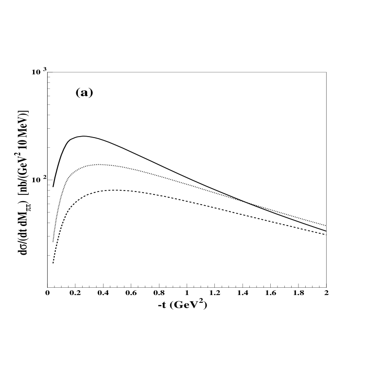
Figure 3(a): Invariant momentum transfer squared distribution for $S$-wave $\pi^{+}\pi^{-}$ photoproduction at $E_{\gamma}^{lab}=4.0\;$ GeV using normal propagators. The solid, dashed, and dotted lines were calculated with $M_{\pi\pi}$ = 0.4, 0.7, and 1.0 GeV, respectively.

Figure 3(b): Invariant momentum transfer squared distribution for $S$-wave $\pi^{+}\pi^{-}$ photoproduction at $E_{\gamma}^{lab}=4.0\;$ GeV using Regge propagators. The solid, dashed, and dotted lines were calculated with $M_{\pi\pi}$ = 0.4, 0.7, and 1.0 GeV, respectively.

Figure 4(a): $S$-wave $\pi^{+}\pi^{-}$ invariant mass distribution at $E_{\gamma}^{lab}=4.0$ GeV and $t=-0.2\;$ GeV² showing sensitivity to the cut-off $\Lambda_{cut}$ using the form factor given by Eq. (31). The solid, dashed, and dotted lines were calculated with $\Lambda_{cut}$ = 0.5, 1.0, and 1.5 GeV, respectively.

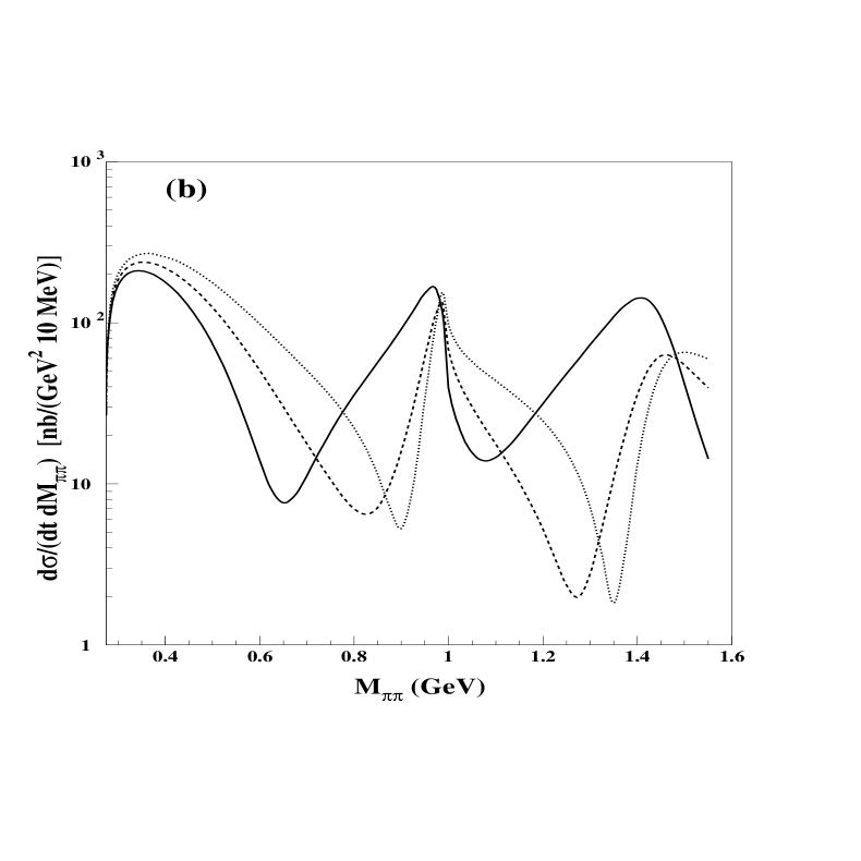
Figure 4(b): $S$-wave $\pi^{+}\pi^{-}$ invariant mass distribution at $E_{\gamma}^{lab}=4.0$ GeV and $t=-0.2\;$ GeV² showing sensitivity to the cut-off $\Lambda_{cut}$ using the form factor given by Eq.(32). The solid, dashed, and dotted lines were calculated with $\Lambda_{cut}$ = 0.5, 1.0, and 1.5 GeV, respectively.

Figure 5(a): $S$-wave $K^{+}K^{-}$ invariant mass distribution at $E_{\gamma}^{lab}=4.0\;$ GeV and $t=-0.2\;$ GeV². Both curves are calculated with no final state interactions (Born cross section). The solid and dashed lines were calculated using Bonn and Spanish parameters, respectively.

Figure 5(b): $S$-wave $K^{+}K^{-}$ invariant mass distribution at $E_{\gamma}^{lab}=4.0\;$ GeV and $t=-0.2\;$ GeV² showing purely on shell FSI terms relative to the Born cross section (dashed line). The solid line shows the FSI result with both $\pi\pi$ and $K\bar{K}$ intermediate channels whereas the dotted line represents the result with no $\pi\pi$ coupling.

Figure 5(c): Expanded $M_{KK}$ range of Fig. 5(b) with the same curve labeling.

Figure 5(d): $S$-wave $K^{+}K^{-}$ invariant mass distribution at $E_{\gamma}^{lab}=4.0\;$ GeV and $t=-0.2\;$ GeV² showing the full FSI terms (on–shell and off–shell) relative to the Born cross section (dashed line). The solid line shows the full FSI result with both $\pi\pi$ and $K\bar{K}$ intermediate channels whereas the dotted line represents the result with no $\pi\pi$ coupling.

Figure 5(e): Expanded $M_{KK}$ range of Fig. 5(d) with the same curve labeling.

Figure 6: t-dependence of the $S$-wave $K^{+}K^{-}$ photoproduction cross section at $E_{\gamma}^{lab}=4.0\;$ GeV with $M_{cut}=1.04\;$ GeV. Solid and dashed lines represent the cross sections with full FSI terms using normal and Regge propagators, respectively. Dotted and dotted-dashed lines represent the Born results using normal and Regge propagators, respectively. Experimental data are taken from Ref. [1].

Figure 7(a): $M_{KK}$ dependence of the $S$-wave $K^{+}K^{-}$ photoproduction cross section at $E_{\gamma}^{lab}=4.0$ GeV with $t_{cut}=-1.5\;$ GeV². Solid and dashed lines represent the cross sections with full FSI terms using normal and Regge propagators, respectively. Dotted and dotted-dashed lines represent the Born results using normal and Regge propagators, respectively.

Figure 7(b): $M_{KK}$ dependence of $S$-wave $K^{+}K^{-}$ photoproduction cross section at $E_{\gamma}^{lab}=4.0$ GeV with $t_{cut}=-0.2\;$ GeV² and the same curve labeling as in Fig. 7(a).

Figure 8(a): Photon energy dependence of the $K\overline{K}$ photoproduction cross section at $M_{KK}=1$ GeV and $t=-0.2$ GeV² (solid line) and $t=-1$ GeV² (dashed line). Normal $\rho$, $\omega$ propagators are used.

Figure 8(b): Same as in Fig. 8(a) but Regge $\rho$, $\omega$ propagators were used.

References

• [1] D. P. Barber et al., Z. Phys. 12, 1 (1982).
• [2] C. D. Fries et al., Nucl. Phys. B143, 408 (1978).
• [3] Electromagnetic Interaction of Hadrons, eds. A Donnachie and G. Shaw, Plenum Press, New York and London, 1978.
• [4] H.-J. Behrend et al., Nucl. Phys. B144, 22 (1978).
• [5] D. Aston et al., Nucl. Phys. B172, 1 (1980).
• [6] Particle Data Group, Phys. Rev. D 54, 557 (1996).
• [7] F. Close, G. R. Farrar and Z. Li, Phys. Rev. D 55, 5749 (1997).
• [8] A. V. Anisovich, V. V. Anisovich and A. V. Sarantsev, Phys. Lett. B395,123 (1997).
• [9] Proceedings of the 14th International Conference on Particles and Nuclei, Williamsburg, USA, 22-28 May 1996, Session 6: Hadron Spectroscopy, edited by C.Carlson and J.Domingo, World Scientific, Singapore, 1996.
• [10] Proceedings of the 28th International Conference on High Energy Physics, Warsaw, Poland, 25-31 July 1996, Session Pa-01: Hadron Spectroscopy, Volume 1, edited by Z.Ajduk and A.K.Wroblewski, World Scientific, Singapore, 1997.
• [11] J. Weinstein and N. Isgur, Phys. Rev. D 27, 588 (1983).
• [12] R. KamiΕ„ski, L. LeΕ›niak and J.-P. Maillet, Phys. Rev. D 50, 3145 (1994).
• [13] R. KamiΕ„ski and L. LeΕ›niak, Phys. Rev. C51, 2264 (1995).
• [14] $N^{*}$ Group of the CLAS Collaboration, CEBAF proposal No. 89-043 (1989).
• [15] M. Atkinson et al., Phys. Lett. 138B, 459 (1984).
• [16] J. A. GΓ³mez Tejedor and E. Oset, Nucl. Phys. A571, 667 (1994).
• [17] C.–R. Ji and S. R. Cotanch, Phys. Rev. D38, 2691 (1988); R. A. Williams, C.-R. Ji and S. R. Cotanch, Phys. Rev. C46, 1617 (1992).
• [18] B. L. G. Bakker, L. A. Kondratyuk and M. V. Terentev, Nucl. Phys. B158, 497 (1979).
• [19] J. A. Oller and E. Oset, Nucl. Phys. A620, 438 (1997).
• [20] R. KamiΕ„ski, L. LeΕ›niak and K. Rybicki, Z. Phys. C74, 79 (1997).
• [21] R. KamiΕ„ski, L. LeΕ›niak and B. Loiseau, Phys. Lett. B413, 130 (1997).
• [22] F. M. Renard, Nuovo Cimento LXII A, 475 (1969).
• [23] H. M. Pilkuhn, Relativistic Particle Physics, Springer-Verlag, New York, 1979.
• [24] S. Rudaz, Phys. Lett. 145B, 281 (1984).
• [25] A. Bramon, A. Grau and G. Pancheri, Phys. Lett. B283, 416 (1992).
• [26] R. Machleidt, K. Holinde and Ch. Elster, Phys. Rep. 149, 1 (1987).
• [27] A. C. Irving and R. P. Worden, Phys. Rep. 34C, 117 (1977).
• [28] S. Nozawa, B. Blankleider and T.-S.H.Lee, Nucl. Phys. A513, 459 (1990).