Abstract
An extended version of the Monte Carlo program GALUGA is presented for the computation of two-photon production in ${\mathrm{e}}^{+}{\mathrm{e}}^{-}$ collisions. Functions implemented for the five $\gamma^{\star}\gamma^{\star}$ structure functions now include several ansätze of the total hadronic cross section based on the BFKL–Pomeron and various Regge-like models. In addition, structure functions for resonance formation are included with full dependence on the two photon virtualities $Q_{1}^{2}$ and $Q_{2}^{2}$ as given in the constituent-quark model. The six lowest-lying resonances of each of the $C$-even mesons with $J^{P}=0^{-}$, $0^{+}$, $1^{+}$, $2^{+}$ and $2^{-}$ are provided. The program can also be used to calculate with exact kinematics the effective two-photon luminosity function. Special emphasis is put on a numerically stable evaluation of all variables over the full $Q_{i}^{2}$ range while keeping all dependences on the electron mass and $Q_{i}^{2}$.

 

^a Heisenberg Fellow.

CERN–TH/97–265
October 1997

Program Summary

Title of program:	GALUGA
Program obtainable from:	G.A. Schuler, CERN–TH,
	CH-1211 Geneva 23, Switzerland;
	Gerhard.Schuler@cern.ch
Licensing provisions:	none
Computer for which the program is designed and others on which it is operable:	all computers
Operating system under which the program has been tested:	UNIX
Programming language used:	FORTRAN 77
Number of lines:	$2209$
Keywords:	Monte Carlo, two-photon, ${\mathrm{e}}^{+}{\mathrm{e}}^{-}$, azimuthal dependence
Subprograms used:	VEGAS [1] (included, 229 lines)
	RANLUX [2] (included, 305 lines)
	HBOOK [3] and DATIME [4] for
	the test program (365 lines)

Nature of physical problem:
Hadronic two-photon reactions in a new energy domain are becoming accessible with LEP2. Unlike purely electroweak processes, hadronic processes contain dominant non-perturbative components parametrized by suitable structure functions, which are functions of the two-photon invariant mass $W$ and the photon virtualities $Q_{1}$ and $Q_{2}$. It is hence advantageous to have a Monte Carlo program that can generate events with the possibility to keep $W$ and, optionally, $Q_{i}$ at fixed, user-defined values. Moreover, at least one program with an exact treatment of both the kinematics and the dynamics over the whole range $m^{2}\gg m^{2}(W/\sqrt{s})^{4}\raisebox{-2.27621pt}{\hskip 2.84526pt$\stackrel{{\scriptstyle<}}{{\sim}}$\hskip 2.84526pt}Q_{i}^{2}\raisebox{-2.27621pt}{\hskip 2.84526pt$\stackrel{{\scriptstyle<}}{{\sim}}$\hskip 2.84526pt}s$ ($m$ is the electron mass and $\sqrt{s}$ the ${\mathrm{e}}^{+}{\mathrm{e}}^{-}$ c.m. energy) is needed, (i) to check the various approximations used in other programs, and (ii) to be able to explore additional information on the hadronic physics, e.g. coded in azimuthal dependences.

Method of solution:
The differential cross section for ${\mathrm{e}}^{+}{\mathrm{e}}^{-}\rightarrow{\mathrm{e}}^{+}{\mathrm{e}}^{-}X$ at given two-photon invariant mass $W$ is rewritten in terms of four invariants with the photon virtualities $Q_{i}$ as the two outermost integration variables (next to $W$), in order to simultaneously cope with antitagged and tagged electron modes. Due care is taken of numerically stable expressions while keeping all electron-mass and $Q_{i}$ dependences. Special attention is devoted to the azimuthal dependences of the cross section. Cuts on the scattered electrons are to a large extent incorporated analytically and suitable mappings introduced to deal with the peaking structure of the differential cross section. The event generation yields either weighted events or unweighted ones (i.e. equally weighted events with weight $1$), the latter based on the hit-or-miss technique. Optionally, VEGAS can be invoked to (i) obtain an accurate estimate of the integrated cross section and (ii) improve the event generation efficiency through additional variable mappings provided by the grid information of VEGAS. The program is set up so that additional hadronic (or leptonic) reactions can easily be added.

Typical running time:
The integration time depends on the required cross-section accuracy and the applied cuts. For instance, $13$ seconds on an IBM RS/6000 yields an accuracy of the VEGAS integration of about $0.1$% for the antitag mode or of about $0.2\%$ for a typical single-tag mode; within the same time the error of the simple Monte Carlo integration is about $0.5$% for either mode. Event generation with or without VEGAS improvement and for either tag mode takes about $4\times 10^{-4}$ ($2\times 10^{-3}$) seconds per event for weighted (unweighted) events.

Differences with earlier version [5]:
i) The $W$-integrated total ${\mathrm{e}}^{+}{\mathrm{e}}^{-}$ cross section $\sigma$ can now be calculated besides ${\mathrm{d}}\sigma/{\mathrm{d}}W^{2}$ and ${\mathrm{d}}^{2}\sigma/{\mathrm{d}}W^{2}{\mathrm{d}}Q_{2}^{2}$.
ii) The program can be used to calculate $\sigma$ for a total, Regge-like hadronic cross section as well as the effective two-photon luminosity function ${\cal L}$ defined by $\sigma=\int{\mathrm{d}}\tau\,{\cal L}(\tau)\,\sigma_{\gamma\gamma}(\tau s)$, where $\sigma_{\gamma\gamma}$ is the real-photon cross section. In both cases four different ansätze for the $Q_{i}$ dependence of the hadronic form factors is provided.
iii) The total two-photon cross section at large $Q_{i}^{2}$ calculated in perturbative QCD, in terms of the BFKL Pomeron, is incorporated.
iv) Structure functions for the formation of resonances in two-photon collisions are included for 30 mesons, light or heavy. One can choose between two models: in one, the full, non-trivial $Q_{1}^{2}$, $Q_{2}^{2}$ correlations as given in the constituent quark model are kept. The alternative model is based on a factorized VMD-inspired ansatz.

1 Introduction

Two-photon physics is facing a revival with the advent of LEP2. Measurements of two-photon processes in a new domain of $\gamma\gamma$ c.m. energies $W$ are ahead of us [6]. Any two-photon process is, in general, described [7] by five non-trivial structure functions (two more for polarized initial electrons). Purely QED (or electroweak) processes are fully calculable within perturbation theory. Several sophisticated Monte Carlo event generators exist [8, 9, 10] to simulate $4$-fermion production in ${\mathrm{e}}^{+}{\mathrm{e}}^{-}$ collisions. Indeed, the differential cross section is not explicitly decomposed as an expansion in the five $\gamma^{\star}\gamma^{\star}$ structure functions. Rather, the full matrix element for the reaction ${\mathrm{e}}^{+}{\mathrm{e}}^{-}\rightarrow{\mathrm{e}}^{+}{\mathrm{e}}^{-}\ell^{+}\ell^{-}$ is calculated as a whole, partly even including QED radiative corrections. Such a procedure is, however, not possible for hadronic two-photon reactions since the hadronic behaviour of the photon is of non-perturbative origin. The decomposition into the above-mentioned five structure functions (and their specification, of course) is hence mandatory for a full description of hadronic reactions.

Monte Carlo event generators for hadronic two-photon processes can be divided into two classes. Programs of the first kind [11, 12, 13, 14, 15, 16] put the emphasis on the QCD part but are (so far) restricted to the scattering of two real photons. The two-photon sub-processes are then embedded in an approximate way in the overall reaction of ${\mathrm{e}}^{+}{\mathrm{e}}^{-}$ collisions. A recent discussion of the so-called equivalent-photon approximation can be found in [17].

The other type of programs [18, 19] treat the kinematics of the vertex ${\mathrm{e}}^{+}{\mathrm{e}}^{-}\rightarrow{\mathrm{e}}^{+}{\mathrm{e}}^{-}\gamma\gamma$ more exactly, but they contain only simple models of the hadronic physics. Moreover, the event generation is done in the variables that are tailored for ${\mathrm{e}}{\mathrm{e}}\rightarrow{\mathrm{e}}{\mathrm{e}}\gamma\gamma$, namely the energies and angles (or virtualities) of the photons and the azimuthal angle $\phi$ between the two lepton-scattering planes in the laboratory system. Hence, both the hadronic energy $W$ and the azimuthal angle $\tilde{\phi}$ in the photon c.m.s. (which enters the decomposition of the ${\mathrm{e}}^{+}{\mathrm{e}}^{-}$ cross section into the five hadronic structure functions) are highly non-trivial functions of these variables.

In the study of hadronic physics one prefers to study events at fixed values of $W$. Not only is $W$ the crucial variable that determines the nature of the hadronic physics (total $\gamma^{\star}\gamma^{\star}$ cross section, resonance formation, etc.), but $\gamma\gamma$ collisions can be compared with $\gamma{\mathrm{p}}$ and ${\mathrm{p}}\overline{{\mathrm{p}}}$ ones through studies of events at fixed $W$ [20]. Next to $W$, the virtualities $Q_{1}$ and $Q_{2}$ of the two photons determine the hadronic physics. At fixed values of $W$ and one of the $Q$’s, say $Q_{1}$, one obtains the cross section of deep-inelastic electron–photon scattering. Varying $Q_{2}$, one can investigate the so-called target-mass effects, i.e. the influence of non-zero values of $Q_{2}$ on the extraction of the photon structure function $F_{2}$. Hence it is desirable to have an event generator that allows keeping $W$ fixed (or integrating over $W$) and in which $Q_{1}$ and $Q_{2}$ are the (next) outermost integration variables, so that $W$ and/or $W$ and $Q_{i}$ can be held constant.

The remaining two non-trivial integration variables, which complete the phase space of ${\mathrm{e}}^{+}{\mathrm{e}}^{-}\rightarrow{\mathrm{e}}^{+}{\mathrm{e}}^{-}X$, should be chosen such that three conditions are fulfilled. First, cuts on the scattered electrons are usually imposed in experimental analyses. Hence, the efficiency and accuracy of the program is improved if these can be treated explicitly rather than incorporated by a simple rejection of those events that fall outside the allowed region. Second, the peaking structure of the differential cross section should be reproduced as well as possible in order to reduce the estimated Monte Carlo error and to improve the efficiency of the event generation. And third, it should be possible to achieve a numerically stable evaluation of all variables needed for a complete event description. These three conditions are met to a large extent by the choice of subsystem squared invariant masses $s_{1}$ and $s_{2}$ as integration variables besides $Q_{1}^{2}$ and $Q_{2}^{2}$. In the laboratory frame, $s_{i}$ are related to the photon energies $\omega_{i}$ by $s_{1/2}-m^{2}=2\omega_{2/1}\sqrt{s}$, where $m$ denotes the electron mass.

In the interest of those readers not interested in calculational details, the paper starts with a presentation of a few results in section 2. The differential cross section for the reaction ${\mathrm{e}}^{+}{\mathrm{e}}^{-}\rightarrow{\mathrm{e}}^{+}{\mathrm{e}}^{-}X$ is rewritten in terms of the four invariants $Q_{i}^{2}$ and $s_{i}$ ($i=1,2$) in section 3 where also models for the cross section $\sigma(\gamma^{\star}\gamma^{\star}\rightarrow X)$ are described. The integration boundaries with $Q_{1}^{2}$ and $Q_{2}^{2}$ as the two outermost integration variables at fixed $W$ are specified in section 4. The derivation of the integration limits is standard [21] but tedious. Here the emphasis is put on numerically stable expressions. To our knowledge, numerical stable forms of $\phi$ and $\tilde{\phi}$ are presented here for the first time. All dependences on the electron mass and the virtualities of the two photons are kept. The formulas are stable over the whole range from $Q_{i\min}^{2}\sim m^{2}(W/\sqrt{s})^{4}\ll m^{2}$ up to $Q_{i\max}^{2}\sim s$, i.e. the program covers smoothly the antitag and tag regions. An equivalent-photon approximation is also implemented (section 5). The complete representation of the four-momenta of the produced particles in terms of the integration variables is given in section 6. Section 7 describes the incorporation of cuts on the scattered electrons. Details of the Monte Carlo program GALUGA are given in section 8.

2 A few results

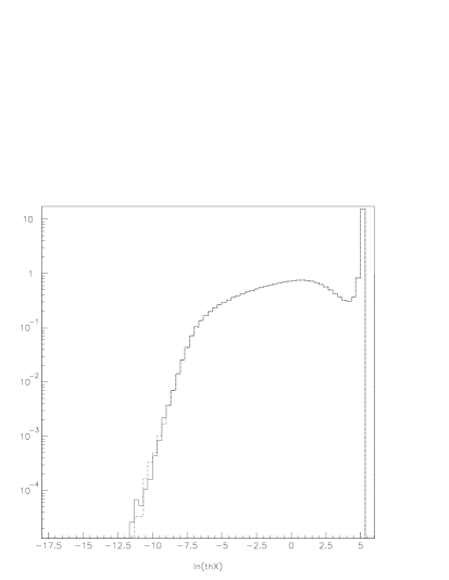
Figure 1: Comparison of muon-pair production in GALUGA (dashed histograms) and DIAG36 (solid histograms) at $\sqrt{s}=130\,$GeV and $W=10\,$GeV. Top: distribution in the logarithm of the polar angle of the $\mu^{+}\mu^{-}$ system; no cuts are applied on the scattered electrons. Bottom: distribution in $t_{1}$ under the cuts: $1.55<\theta_{1}<3.67^{\circ}$ and $30\,$GeV$<E_{1}$.

In order to check GALUGA, we include the production of lepton pairs, for which several well-established Monte Carlo generators [8, 9, 10] exist. The five structure functions for $\gamma^{\star}\gamma^{\star}\rightarrow\ell^{+}\ell^{-}$ as quoted in [7] have been implemented. For the comparison we have modified the two-photon part of the four-fermion program DIAG36 [9] (i.e. DIAG36 restricted to the multiperipheral diagrams) in such a way that it can produce events at fixed values of $W$. The agreement is excellent. Two examples are shown in Fig. 1, the first corresponding to a no-tag setup and the second to a single tagging mode.

Next we study the (integrated) total hadronic cross section. Figures 2 and 3–5 compare different ansätze for the $Q_{i}^{2}$ behaviour of the various cross sections for transverse and longitudinal photons. The results of the two models of generalized-vector-meson-dominance type (GVMD (17) and VMDc (18), dash-dotted and dotted histograms, respectively) are hardly distinguishable in the no-tag case, but may deviate by more than $20\%$ in a single-tag case. In the contrast, the different $Q_{i}^{2}$ behaviour of a simple $\rho$-pole (dashed histograms) shows up already in the no-tag mode. Note that this model includes scalar photon contributions, but does not possess an $1/Q^{2}$ “continuum” term for transverse photons. These differences imply that effects of non-zero $Q_{i}^{2}$ values must not be neglected for a precision measurement of $\sigma_{\gamma\gamma}(W^{2})$.

During the course of the LEP2 workshop, sophisticated programs to generate the full (differential) hadronic final state in two-photon collisions have been developed [22]. The description of hadronic physics with one (or both) photons off-shell by virtualities $Q_{i}^{2}\ll W^{2}$ is still premature. Indeed, existing programs are thus far for real photons and hence use, in one way or another, the equivalent-photon approximation (EPA) to embed the two-photon reactions in the ${\mathrm{e}}^{+}{\mathrm{e}}^{-}$ environment. It is hence indispensable to check the uncertainties associated with the EPA. Hadronic physics is under much better theoretical control for deep-inelastic scattering, i.e. the setup of one almost real photon probed by the other that is off-shell by an amount $Q^{2}$ of the order of $W^{2}$. Corresponding event generators exist [22] but also in this case it is desirable to check the equivalent-photon treatment of the probed photon.

An improved EPA has recently been suggested in [17]. In essence, the prescription consists in neglecting $Q_{i}^{2}$ w.r.t. $W^{2}$ in the kinematics but to keep the full $Q_{i}^{2}$ dependence in the $\gamma^{\star}\gamma^{\star}$ structure functions. In addition, non-logarithmic terms proportional to $m^{2}/Q_{i}^{2}$ in the luminosity functions are kept as well. The study [17] shows that this improved EPA works rather well for the integrated ${\mathrm{e}}^{+}{\mathrm{e}}^{-}$ cross section. In Fig. 2 we show that this EPA (solid compared to dash-dotted histograms) works well also for differential distributions, with the exception of the polar-angle distribution of the hadronic system at large angles, where it can, in fact, fail by more than an order of magnitude! (There, of course, the cross section is down by several orders.)

The EPA describes also rather well the dynamics of the scattered electrons in the single-tag mode except in the tails of the distributions (Fig. 3). The same holds for the distributions in the photon virtualities, see Fig. 4. Sizeable differences do, however, show up (Fig. 4) in the distributions of the subsystem invariant masses $\sqrt{s_{i}}$. These then lead to the wrong shapes for the energy and momentum distributions of the hadronic system shown in Fig. 5. The EPA should, therefore, not be used for single-tag studies.

Finally we study the prospects of a determination of additional structure functions besides $F_{2}$. One such possibility was outlined in [6], namely the study of the azimuthal dependence in the $\gamma\gamma$ c.m.s. between the plane of the scattered (tagged) electron and the plane spanned by the beam axis and the outgoing muon or jet. Here we propose to study the azimuthal angle $\tilde{\phi}$ between the two electron scattering planes, again in the $\gamma\gamma$ c.m.s. Although such a study requires a double-tag setup, the event rates need not be small, since one can fully integrate out the hadronic system but for its invariant mass $W$. In order to demonstrate the sensitivity of such a measurement we show, as a preparatory exercise, the $\tilde{\phi}$ distribution for muon-pair production in Fig. 6. Fitting to the functional form

$$\frac{{\mathrm{d}}\sigma}{{\mathrm{d}}\tilde{\phi}}\propto 1+A_{1}\,\cos\tilde{\phi}+A_{2}\,\cos 2\,\tilde{\phi}\ ,$$ (1)

we find

$$A_{1}=0.098\qquad,\qquad A_{2}=-0.028\ .$$ (2)

Let us emphasize that the selected tagging ranges have in no way been optimized for such a study. Nonetheless, given the magnitudes of $A_{i}$, a measurement appears feasible.

All but one [8] event generators for two-photon physics use the azimuthal angle $\phi$ between the two scattering planes in the laboratory frame as one of the integration variables. In fact, $\phi$ appears as a trivial variable in these programs. None of these up to now provides the calculation of $\tilde{\phi}$. An expression for $\tilde{\phi}$ in terms of $t_{i}$, $\phi$, and two other invariants is given in [7] (see (55) below) and, in principle, is available in TWOGAM [18]. However, the factor $\sqrt{t_{1}t_{2}}$ appears explicitly in the denominator of $\cos\tilde{\phi}$ but not in its numerator. Hence, at small values of $-t_{i}$ this factor will be the result of the cancellation of several much larger terms, rendering this expression for $\cos\tilde{\phi}$ numerically very unstable. (Recall that $|t_{i}|_{\min}\sim m^{2}(W/\sqrt{s})^{4}\ll m^{2}$, while the numerator contains terms of order $s$.) In contrast, we use the numerically stable expression given in (56).

An approximation for $\tilde{\phi}$ in terms of $\phi$ is proposed in [23]:

$$\cos\tilde{\phi}_{\mathrm{approx}}=\cos\phi+\sin^{2}\phi\,\frac{Q_{1}\,Q_{2}\,(2\,s-s_{1}-s_{2})}{(W^{2}-t_{1}-t_{2})\sqrt{(s-s_{1})(s-s_{2})}}\ .$$ (3)

Indeed, the correlation between $\tilde{\phi}$ and its approximation is very high in the no-tag case, where, however, the dependence on $\tilde{\phi}$ is almost trivial (i.e. flat). Figure 6 exhibits that there is still a correlation for a double-tag mode, but formula (3) fails to reproduce the correct $\tilde{\phi}$ dependence: a fit to (1) yields $A_{1}=0.084$ and $A_{2}=0.017$, quite different from (2).

3 Notation and cross sections

Consider the reaction

$${\mathrm{e}}^{+}(p_{a})+{\mathrm{e}}^{-}(p_{b})\rightarrow{\mathrm{e}}^{+}(p_{1})+X(p_{X})+{\mathrm{e}}^{-}(p_{2})$$ (4)

proceeding through the two-photon process

$$\gamma(q_{1})+\gamma(q_{2})\rightarrow X(p_{X})\ .$$ (5)

The cross section for (4) depends on six invariants, which we choose to be the ${\mathrm{e}}^{+}{\mathrm{e}}^{-}$ c.m. energy $\sqrt{s}$, the $\gamma\gamma$ c.m. (or hadronic) energy $W$, the photon virtualities $Q_{i}$, and the subsystem invariant masses $\sqrt{s_{i}}$:

$$\,s=(p_{a}+p_{b})^{2} \quad,\quad W^{2}=p_{X}^{2}\ ,$$

$$s_{1}=(p_{1}+p_{X})^{2}=(p_{a}+q_{2})^{2} \quad,\quad-Q_{1}^{2}=t_{1}=q_{1}^{2}\equiv(p_{a}-p_{1})^{2}\ ,$$

$$s_{2}=(p_{2}+p_{X})^{2}=(p_{b}+q_{1})^{2} \quad,\quad-Q_{2}^{2}=t_{2}=q_{2}^{2}\equiv(p_{b}-p_{2})^{2}\ .$$ (6)

We find it convenient to introduce also the dependent variables:

$$u_{2}=s_{1}-m^{2}-t_{2} \quad,\quad\nu=\frac{1}{2}\,\left(W^{2}-t_{1}-t_{2}\right)\ ,$$

$$u_{1}=s_{2}-m^{2}-t_{1} \quad,\quad K=\frac{1}{2\,W}\,\sqrt{\lambda(W^{2},t_{1},t_{2})}=\frac{1}{W}\,\sqrt{\nu^{2}-t_{1}\,t_{2}}\ ,$$

$$\,\beta=\sqrt{1-\frac{4m^{2}}{s}} \quad,\quad y_{i}=\sqrt{1-\frac{4m^{2}}{t_{i}}}\ ,$$ (7)

where $\lambda(x,y,z)=(x-y-z)^{2}-4yz$ and $m$ denotes the electron mass. Note that $K$ is the photon three-momentum in the $\gamma\gamma$ c.m.s. In terms of these variables the ${\mathrm{e}}^{+}{\mathrm{e}}^{-}$ cross section at fixed values of $\sqrt{s}$ and $\tau=W^{2}/s$ is given by:

$$\frac{{\mathrm{d}}\sigma[{\mathrm{e}}^{+}{\mathrm{e}}^{-}\rightarrow{\mathrm{e}}^{+}+{\mathrm{e}}^{-}+X]}{{\mathrm{d}}\tau}=\frac{\alpha^{2}\,K\,W}{2\,\pi^{4}\,Q_{1}^{2}\,Q_{2}^{2}\beta}\,{\mathrm{d}}R_{3}\,\Sigma(W^{2},Q_{1}^{2},Q_{2}^{2},s_{1},s_{2},\tilde{\phi};s,m^{2})\ ,$$ (8)

where $R_{3}$ is the phase space for (4).

We also give the relation between the cross section at fixed values of $\tau$ and $Q_{2}^{2}$ and the usual form used in deep-inelastic scattering:

$$\frac{{\mathrm{d}}\sigma}{{\mathrm{d}}\tau\,{\mathrm{d}}t_{2}}=\frac{x^{2}\,s}{Q_{2}^{2}}\,\frac{{\mathrm{d}}\sigma}{{\mathrm{d}}x\,{\mathrm{d}}Q_{2}^{2}}\ ,$$ (9)

where $x$ is the Bjorken-$x$ variable defined by

$$x=\frac{Q_{2}^{2}}{2\,q_{1}\cdot q_{2}}=\frac{Q_{2}^{2}}{W^{2}+Q_{2}^{2}+Q_{1}^{2}}\ .$$ (10)

The hadronic physics is fully encoded in five structure functions. Three of these can be expressed through the cross sections $\sigma_{ab}$ for scalar ($a,b=S$) and transverse photons ($a,b=T$) ($\sigma_{ST}=\sigma_{TS}(q_{1}\leftrightarrow q_{2})$). The other two structure functions $\tau_{TT}$ and $\tau_{TS}$ correspond to transitions with spin-flip for each of the photons with total helicity conservation. Introducing $\tilde{\phi}$, the angle between the scattering planes of the colliding ${\mathrm{e}}^{+}$ and ${\mathrm{e}}^{-}$ in the photon c.m.s., these structure functions enter the cross sections as:

$$\Sigma = 2\,\rho_{1}^{++}\,2\,\rho_{2}^{++}\,\sigma_{TT}+2\,\rho_{1}^{++}\,\rho_{2}^{00}\,\sigma_{TS}+\rho_{1}^{00}\,2\,\rho_{2}^{++}\,\sigma_{ST}+\rho_{1}^{00}\,\rho_{2}^{00}\,\sigma_{SS}$$ (11)

$$+~{}2\,|\rho_{1}^{+-}\,\rho_{2}^{+-}|\,\tau_{TT}\,\cos 2\,\tilde{\phi}-8\,|\rho_{1}^{+0}\,\rho_{2}^{+0}|\,\tau_{TS}\,\cos\tilde{\phi}\ .$$

The density matrices of the virtual photons in the $\gamma\gamma$-helicity basis are given by

$$2\,\rho_{1}^{++} = \frac{\left(u_{2}-\nu\right)^{2}}{K^{2}\,W^{2}}+1+\frac{4\,m^{2}}{t_{1}}$$

$$\rho_{1}^{00} = \frac{\left(u_{2}-\nu\right)^{2}}{K^{2}\,W^{2}}-1$$

$$|\rho_{1}^{+-}| = \rho_{1}^{++}-1$$

$$|\rho_{1}^{+0}| = \sqrt{\left(\rho_{1}^{00}+1\right)|\rho_{1}^{+-}|}=\frac{u_{2}-\nu}{K\,W}\,\sqrt{\rho_{1}^{++}-1}$$ (12)

with analogous formulas for photon $2$.

A few remarks about the numerical stability of the $\tilde{\phi}$-dependent terms are in order. Thus far, these terms are implemented solely in the TWOGAM [18] event generator, using the formulas quoted in [7]. Given in [7] and coded in [18] are the products $X_{2}=2\,|\rho_{1}^{+-}\,\rho_{2}^{+-}|\,\cos 2\,\tilde{\phi}$ and $X_{1}=8\,|\rho_{1}^{+0}\,\rho_{2}^{+0}|\,\cos\tilde{\phi}$ in terms of invariants. Now, the expressions for $X_{i}$ contain explicit factors of $t_{1}t_{2}$ ($X_{2}$) and $\sqrt{t_{1}t_{2}}$ ($X_{1}$) in the denominators but not in the numerators. Clearly, the evaluation of $X_{i}$ becomes unstable for small values of $|t_{i}|$. On the other hand, the factors multiplying $\cos\tilde{\phi}$ and $\cos 2\tilde{\phi}$ in $X_{i}$ approach perfectly stable expressions in the limit $m^{2}/W^{2}\rightarrow 0$ and $t_{i}/W^{2}\rightarrow 0$:

$$|\rho_{1}^{+-}| \rightarrow \frac{2}{x_{1}^{2}}\,(1-x_{1})+\frac{2\,m^{2}}{t_{1}}$$

$$|\rho_{1}^{+0}| \rightarrow \frac{2-x_{1}}{x_{1}}\,\sqrt{|\rho_{1}^{+-}|}\ ,$$ (13)

where $x_{i}=W^{2}/s_{i}\approx s_{k}/s$ ($i\neq k$). Hence a numerically stable evaluation of $\tilde{\phi}$ guarantees a correct evaluation of the $\tilde{\phi}$-dependent terms.

The structure functions $\sigma_{ab}$ and $\tau_{ab}$ for lepton-pair production are often quoted in the literature; the formulas of [7] are implemented in the program. Much less is known about the structure functions for hadronic processes. Since we are not aware of a model for $\tau_{ab}$ of the total hadronic cross section, the current version of the program assumes

$$\tau_{TT}=0=\tau_{TS}\ .$$ (14)

The program is set up in such a way that it is straightforward to add a model for $\tau_{ab}$. For resonance production, $\tau_{ab}$ as given in the constituent quark model are implemented.

The $Q_{i}$ dependence of the cross sections $\sigma_{ab}$ reflects the hadronic physics of the process under consideration. For the total hadronic cross section, four Regge-based models are provided. They are based upon the assumption

$$\sigma_{ab}(W^{2},Q_{i}^{2})=h_{a}(Q_{1}^{2})\,h_{b}(Q_{2}^{2})\,\sigma_{\gamma\gamma}(W^{2})\ ,$$ (15)

which is valid for $Q_{i}^{2}\ll W^{2}$; this is justified in most applications. Note the cross section for the scattering of two real photons $\sigma_{\gamma\gamma}(W^{2})$ that enters as a multiplicative factor in (15). We take it as [20]

$$\sigma_{\gamma\gamma}(W)=X\,s^{\epsilon}+Y\,s^{-\eta}\ .$$ (16)

The program can be used to calculate a two-photon luminosity function if one takes $\sigma_{\gamma\gamma}(W)=1$.

The four models are defined as follows. The first one is based upon a parametrization [24] of the $\gamma^{*}{\mathrm{p}}$ cross section calculated in a model of generalized vector-meson dominance (GVMD):

$$h_{T}(Q^{2}) = r\,P_{1}^{-2}(Q^{2})+(1-r)\,P_{2}^{-1}(Q^{2})$$

$$h_{S}(Q^{2}) = \xi\,\left\{r\,\frac{Q^{2}}{m_{1}^{2}}\,P_{1}^{-2}(Q^{2})+(1-r)\,\left[\frac{m_{2}^{2}}{Q^{2}}\,\ln P_{2}(Q^{2})-P_{2}^{-1}(Q^{2})\right]\right\}$$

$$P_{i}(Q^{2}) = 1+\frac{Q^{2}}{m_{i}^{2}}\ ,$$ (17)

where we take $\xi=1/4$, $r=3/4$, $m_{1}^{2}=0.54\,$GeV² and $m_{2}^{2}=1.8\,$GeV².

The second model [25] adds a continuum contribution to simple (diagonal, three-mesons only) vector–meson dominance (VMDc):

$$h_{T}(Q^{2}) = \sum_{V=\rho,\omega,\rho}\,r_{V}\,\left(\frac{m_{V}^{2}}{m_{V}^{2}+Q^{2}}\right)^{2}+r_{c}\,\frac{m_{0}^{2}}{m_{0}^{2}+Q^{2}}$$

$$h_{S}(Q^{2}) = \sum_{V=\rho,\omega,\rho}\,\frac{\xi\,Q^{2}}{m_{V}^{2}}\,r_{V}\,\left(\frac{m_{V}^{2}}{m_{V}^{2}+Q^{2}}\right)^{2}\ ,$$ (18)

where $r_{\rho}=0.65$, $r_{\omega}=0.08$, $r_{\phi}=0.05$, and $r_{c}=1-\sum_{V}r_{V}$.

Since photon-virtuality effects are often estimated by using a simple $\rho$-pole only, we include also the model defined by ($\rho$-pole):

$$h_{T}(Q^{2})=\left(\frac{m_{\rho}^{2}}{m_{\rho}^{2}+Q^{2}}\right)^{2}\qquad,\qquad h_{S}(Q^{2})=\frac{\xi\,Q^{2}}{m_{\rho}^{2}}\,\left(\frac{m_{\rho}^{2}}{m_{\rho}^{2}+Q^{2}}\right)^{2}\ .$$ (19)

The fourth model is identical to (19) but has $h_{S}(Q^{2})=0$.

At large virtualities the behaviour of the $\gamma^{\star}\gamma^{\star}$ cross sections is fully predicted by perturbative QCD in terms of the BFKL Pomeron [26]. We use the results obtained in the so-called saddle-point approximation

$$\sigma_{ab}=W_{a}\,W_{b}\,\left(\sum_{f}q_{f}^{2}\right)^{2}\,\frac{\alpha^{2}_{em}\,\alpha_{s}^{2}\,\pi^{9/2}}{256\,Q_{1}\,Q_{2}}\,\frac{\exp\left(4\,\xi\,\ln 2\right)}{\sqrt{14\,\xi\,\zeta(3)}}\,\exp\left(-\frac{\ln^{2}(Q_{1}^{2}/Q_{2}^{2})}{56\,\xi\,\zeta(3)}\right)\ ,$$ (20)

where $W_{T}=9$, $W_{L}=2$, and

$$\xi = \frac{N_{c}\,\alpha_{s}}{\pi}\,\ln\frac{W^{2}}{Q^{2}}\ ,\qquad Q^{2}=c_{Q}\,Q_{1}\,Q_{2}\ ,\qquad c_{Q}=10^{2}$$

$$\alpha_{s} = \frac{12\,\pi}{(33-2\,n_{f})\,\ln(\mu^{2}/\Lambda^{2})}\ ,\qquad\mu^{2}=c_{\mu}\,Q_{1}\,Q_{2}\qquad(c_{\mu}=\exp(-5/3))\ .$$ (21)

In order to ensure the validity of the high-energy approximation that went into the calculation of [26] we demand

$$Q_{\mathrm{min}}<Q_{i}<Q_{\mathrm{max}}\ ,\qquad W^{2}>\delta\,Q_{1}\,Q_{2}\quad(\delta=10^{2})\ .$$ (22)

$i\backslash j$		$1$	$2$	$3$	$4$	$5$
	$n\,{}^{2S+1}L_{J}$	$I=1$	$I=0$	$(I=0)^{\prime}$	$c\bar{c}$	$b\bar{b}$
$1$	$1\,{}^{1}S_{0}$	$\pi^{0}$	$\eta$	$\eta^{\prime}$	$\eta_{c}$	$[\eta_{b}(9400)]$
$2$	$1\,{}^{3}P_{0}$	$a_{0}(980)^{\star}$	$f_{0}(980)^{\star}$	$f_{0}(1370)^{\star}$	$\chi_{c_{0}}$	$\chi_{b_{0}}$
$3$	$1\,{}^{3}P_{1}$	$a_{1}(1260)$	$f_{1}(1285)$	$f_{1}(1510)$	$\chi_{c_{1}}$	$\chi_{b_{1}}$
$4$	$1\,{}^{3}P_{2}$	$a_{2}(1320)$	$f_{2}(1270)$	$f_{2}^{\prime}(1525)$	$\chi_{c_{2}}$	$\chi_{b_{2}}$
$5$	$1\,{}^{1}D_{2}$	$\pi_{2}(1670)$	$[\eta_{D}(1680)]$	$[\eta_{D}^{\prime}(1890)]$	$[\eta_{c_{D}}(3840)]$	$[\eta_{b_{D}}(10150)]$
$6$	$2\,{}^{1}S_{0}$	$\pi(1300)$	$\eta(1295)$	$[\eta^{\prime}(1400)]$	$\eta_{c}(2S)$	$[\eta_{b}(9980)]$

Table 1: Lowest-lying $C=+1$ mesons [28] and their labelling with $i$ and $j$. States in brackets are not yet found. Status of states marked with a $\star$ is not yet clarified.

Structure functions for resonance formation in two-photon fusion were recently calculated in the constituent-quark model [27]. Although the results stricly apply to heavy mesons only, the $Q_{i}$ dependence is presumably also very reasonable for the lighter mesons. The mesons included are listed in Table 1. The structure functions are given by

$$\sigma_{ab}[J^{P}]=(2J+1)\,8\,\pi^{2}\,\frac{\tilde{\Gamma}_{\gamma\gamma}}{M}\,f_{ab}(Q_{1},Q_{2},M_{p};J^{P})\,{\mathrm{BW}}\,(W,M)\ .$$ (23)

Here $M$ denotes the mass, $J$ the total spin, $P$ the parity, and $\Gamma$ the total width of the $C=+1$ meson. The mass $M_{p}$ is equal to $M$ for all mesons except for $\pi^{0}$, $\eta$, and $\eta^{\prime}$, for which we take the $\rho$ mass. $\tilde{\Gamma}_{\gamma\gamma}$ is the two-photon decay width for all mesons except for those with $J=1$, where a different quantity had to be introduced since $J=1$ mesons cannot decay into two real photons. Explicit expressions for $\tilde{\Gamma}_{\gamma\gamma}$ and $f_{ab}$ can be found in [27]. Form factors for the interference terms $\tau_{TT}$ and $\tau_{TS}$ are also implemented. The $W$ dependence is given by

$${\mathrm{BW}}\,(W,M) = \frac{1}{\pi}\,\frac{M\,\Gamma}{(M^{2}-W^{2})^{2}+M^{2}\,\Gamma^{2}}$$ (24)

$$= \delta(W^{2}-M^{2})\ ,$$

depending on whether one integrates over $W$ or keeps $W$ fixed.

Note that the form factors $f_{ab}(Q_{1},Q_{2},M_{p};J^{P})$ do not factor in $Q_{1}$- and $Q_{2}$-dependent factors, nor do they have simple monopole or dipole behaviours. As an alternative a simple factorizing model based on VMD is also implemented

$$\sigma_{ab}[J^{P}]=(2J+1)\,8\,\pi^{2}\,\frac{\Gamma_{\gamma\gamma}}{M}\,\left(\frac{m_{\rho}^{2}}{m_{\rho}^{2}+Q_{1}^{2}}\right)^{2}\left(\frac{m_{\rho}^{2}}{m_{\rho}^{2}+Q_{2}^{2}}\right)^{2}\,{\mathrm{BW}}\,(W,M)\ .$$ (25)

Observe that all $1^{+}$ cross sections are zero for model (25).

4 Phase space

The phase space can be expressed in terms of four invariants:

$${\mathrm{d}}R_{3} \equiv \prod_{i=1,2,X}\,\int\,\frac{{\mathrm{d}}^{3}p_{i}}{2\,E_{i}}\,\delta^{4}\left(p_{a}+p_{b}-\sum_{i}\,p_{i}\right)$$ (26)

$$= \frac{1}{16\,\beta\,s}\,\int\,{\mathrm{d}}t_{2}\,{\mathrm{d}}t_{1}\,{\mathrm{d}}s_{1}\,{\mathrm{d}}s_{2}\,\frac{\pi}{\sqrt{-\Delta_{4}}}\ ,$$

where $\Delta_{4}$ is the $4\times 4$ symmetric Gram determinant of any four independent vectors formed out of $p_{a}$, $p_{b}$, $p_{1}$, $p_{X}$, $p_{2}$. The physical region in $t_{2}$, $t_{1}$, $s_{1}$, $s_{2}$ for fixed $s$ satisfies $\Delta_{4}\leq 0$. Since $\Delta_{4}$ is a quadratic polynomial in any of its arguments, the boundary of the physical region, $\Delta_{4}=0$, is a quadratic equation and has two solutions. Picking $s_{2}$ as the innermost integration variable, the explicit evaluation of $\Delta_{4}$ yields

$$16\,\Delta_{4}=a\,s_{2}^{2}+b\,s_{2}+c=a\,(s_{2}-s_{2+})\,(s_{2}-s_{2-})\ ,$$ (27)

where

$$a = \lambda(s_{1},t_{2},m^{2})$$

$$b = -2\,s\ {m}^{2}t_{1}-2\,{m}^{2}s_{1}^{2}+8\,t_{2}\,{m}^{4}-2\,{m}^{2}t_{2}^{2}-2\,s\ s_{1}\,{W}^{2}+2\,{m}^{2}s\ {W}^{2}+2\,t_{1}\,s\ s_{1}+2\,s\ t_{2}\,s_{1}$$

$$~{}+4\,{m}^{2}s_{1}\,{W}^{2}+4\,{m}^{4}s_{1}+2\,t_{1}\,t_{2}\,s-2\,t_{2}\,{m}^{2}t_{1}-2\,t_{2}^{2}s-2\,{m}^{2}t_{2}\,s+2\,t_{1}\,t_{2}\,s_{1}$$

$$~{}-4\,{m}^{4}{W}^{2}-2\,t_{1}\,s_{1}^{2}+2\,s\ t_{2}\,{W}^{2}-2\,{m}^{6}+2\,{m}^{4}t_{1}$$

$$c = -2\,s\ {m}^{4}{W}^{2}-2\,t_{1}^{2}{m}^{2}s_{1}-2\,t_{1}\,t_{2}\,{s}^{2}+2\,s\ t_{1}\,t_{2}\,s_{1}-2\,s\ t_{1}^{2}s_{1}+t_{1}^{2}{s}^{2}+t_{1}^{2}s_{1}^{2}+t_{2}^{2}{s}^{2}$$ (28)

$$~{}+{m}^{4}s_{1}^{2}+{m}^{4}t_{1}^{2}-6\,{m}^{6}t_{1}-2\,{m}^{6}s_{1}-4\,{m}^{4}s_{1}\,{W}^{2}+2\,{m}^{4}t_{2}\,s+2\,{m}^{4}t_{2}\,s_{1}+8\,{m}^{4}t_{1}\,s_{1}$$

$$~{}-2\,{s}^{2}t_{2}\,{W}^{2}-2\,t_{1}\,{s}^{2}{W}^{2}-2\,{m}^{2}t_{1}\,s_{1}^{2}+{m}^{8}-2\,{m}^{2}s\ t_{2}\,s_{1}+4\,{m}^{6}{W}^{2}+{m}^{4}t_{2}^{2}$$

$$~{}+4\,{m}^{2}t_{1}\,t_{2}\,s-2\,{m}^{2}t_{1}\,t_{2}\,s_{1}-6\,{m}^{6}t_{2}+{s}^{2}{W}^{4}+6\,{m}^{2}s\ t_{2}\,{W}^{2}-4\,s\ {m}^{2}{W}^{4}$$

$$~{}-2\,s\ {m}^{2}t_{1}^{2}+2\,s\ t_{1}\,{m}^{4}-2\,s\ {m}^{2}t_{2}^{2}+2\,t_{1}\,t_{2}\,{m}^{4}+2\,s\ {m}^{2}s_{1}\,{W}^{2}-4\,s\ t_{1}\,t_{2}\,{W}^{2}$$

$$~{}-2\,s\ t_{1}\,{m}^{2}s_{1}+6\,s\ t_{1}\,{m}^{2}{W}^{2}+2\,s\ t_{1}\,s_{1}\,{W}^{2}\ .$$

A numerical stable form for the $s_{2}$ limits is

$$s_{2+} = \frac{-b+\sqrt{\Delta}}{2\,a}$$

$$s_{2-} = \frac{c}{a\,s_{2+}}\ ,$$ (29)

where $\Delta=b^{2}-4\,a\,c$ is given below in a numerically stable form, in (32).

In order to remove the singularity due to $(-\Delta_{4})^{-1/2}$ (in the limit $|t_{i}|$, $m^{2}\ll s_{i}$, $W^{2}$, the $s_{2}$ integration degenerates to an integration over the $\delta$-function $\delta(s_{2}-s\,W^{2}/s_{1})$), it is advisable to change variable from $s_{2}$ to $x_{4}$, $0\leq x_{4}\leq 1$:

$$s_{2} = \frac{1}{2\,a}\,\left\{-b-\sqrt{\Delta}\,\cos\left(x_{4}\,\pi\right)\right\}$$

$$\int_{s_{2-}}^{s_{2+}}\,\frac{{\mathrm{d}}s_{2}}{\sqrt{-\Delta_{4}}} = \frac{4\,\pi}{\sqrt{a}}\,\int_{0}^{1}\,{\mathrm{d}}x_{4}\ .$$ (30)

For later use we also need a numerically stable form of the Gram determinant, which reads

$$16\,\Delta_{4}=-\frac{\Delta\,\sin^{2}\left(x_{4}\,\pi\right)}{4\,a}\ .$$ (31)

The $s_{1}$-integration limits follow from the requirement $\Delta>0$. They are most easily derived when realizing that the discriminant $\Delta$ is given as the product of two $3\times 3$ symmetric Gram determinants or, equivalently, the product of two kinematic $G$ functions

$$\frac{1}{4}\,\Delta=4\,G_{3}\,G_{4}=64\,D_{3}\,D_{4}\ ,$$ (32)

where

$$-4\,D_{3}\equiv-4\,\Delta_{3}(p_{a},p_{b},q_{2}) = G(s,t_{2},s_{1},m^{2},m^{2},m^{2})\equiv G_{3}$$

$$-4\,D_{4}\equiv-4\,\Delta_{3}(p_{a},q_{1},q_{2}) = G(t_{1},s_{1},t_{2},m^{2},m^{2},W^{2})\equiv G_{4}\ .$$ (33)

Since any $3\times 3$ Gram determinant $\Delta_{3}$ satisfies $\Delta_{3}\geq 0$, the physical region is that where both $G_{3}$ and $G_{4}$ are simultaneously negative. Solving $G_{i}$ for $s_{1}$

$$G_{3} = m^{2}\,(s_{1}-s_{11+})\,(s_{1}-s_{11-})$$

$$= {m}^{2}s_{1}^{2}-2\,{m}^{4}s_{1}-s\ t_{2}\,s_{1}-3\,{m}^{2}t_{2}\,s\ +{m}^{6}+t_{2}\,{s}^{2}+t_{2}^{2}s$$

$$G_{4} = t_{1}\,(s_{1}-s_{12+})\,(s_{1}-s_{12-})$$ (34)

$$= -2\,t_{1}\,{m}^{2}s_{1}-t_{2}\,{m}^{2}t_{1}+{m}^{4}t_{1}-{m}^{2}{W}^{2}t_{1}+{m}^{2}t_{2}^{2}+t_{2}\,{W}^{2}t_{1}-t_{1}\,s_{1}\,{W}^{2}$$

$$~{}-2\,{m}^{2}t_{2}\,{W}^{2}+{m}^{2}{W}^{4}+t_{1}\,s_{1}^{2}+t_{1}^{2}s_{1}-t_{1}\,t_{2}\,s_{1}$$

we find

$$s_{11\pm} = {\frac{t_{2}\,S+2\,{m}^{4}\pm\sqrt{\lambda(S,{m}^{2},{m}^{2})\lambda(t_{2},{m}^{2},{m}^{2})}}{2\,{m}^{2}}}$$

$$s_{12\pm} = {\frac{t_{2}}{2}}+{m}^{2}+{\frac{{W}^{2}}{2}}-{\frac{t_{1}}{2}}\pm{\frac{\sqrt{\lambda(t_{1},t_{2},{W}^{2})\lambda(t_{1},{m}^{2},{m}^{2})}}{2\,t_{1}}}$$

$$s_{11+}s_{11-} = {\frac{t_{2}\,S\left(-3\,{m}^{2}+S+t_{2}\right)}{{m}^{2}}}+{m}^{4}$$

$$s_{12+}s_{12-} = \left(W^{2}-m^{2}\right)\,\left(-{m}^{2}+t_{2}\right)+{\frac{{m}^{2}\left({W}^{2}-t_{2}\right)^{2}}{t_{1}}}\ .$$ (35)

Note that $s_{12+}\leq s_{12-}$. Since $G_{3}$ is always negative between its two roots, the range of integration over $s_{1}$ is $s_{12-}\leq s_{1}\leq s_{11+}$. Numerically it is more advantageous to calculate the limits as

$$s_{1\min} = s_{12-}=m^{2}+\frac{1}{2}\,\left(W^{2}-t_{1}+t_{2}+y_{1}\ \sqrt{\lambda(W^{2},t_{1},t_{2})}\right)$$

$$s_{1\max} = s_{11+}=m^{2}+\frac{2\ (s+t_{2}-4\ m^{2})}{1+\beta\ y_{2}}\ .$$ (36)

The dominant behaviour of the $s_{1}$ integration is given by the factor $\lambda^{-1/2}(s_{1},t_{2},m^{2})$, see (30). (In the limit $t_{2}$, $m^{2}\ll s_{1}$, this becomes ${\mathrm{d}}s_{1}/s_{1}$ integration.) This factor can be transformed away by the variable transformation from $s_{1}$ to $x_{3}$, $0\leq x_{3}\leq 1$,

$$s_{1} = X_{1}/2+m^{2}+t_{2}+2\,m^{2}\,t_{2}/X_{1}$$

$$X_{1} = (\nu+K\,W)\,(1+y_{1})\,\exp{(\delta_{1}\,x_{3})}$$

$$\delta_{1} = \ln\frac{s\,(1+\beta)^{2}}{(\nu+K\,W)\,(1+y_{1})\,(1+y_{2})}\ ,$$ (37)

such that

$$\int_{s_{1\min}}^{s_{1\max}}\,{\mathrm{d}}s_{1}\,\frac{4\,\pi}{\sqrt{a}}=4\,\pi\,\delta_{1}\,\int_{0}^{1}\,{\mathrm{d}}x_{3}\ .$$ (38)

The physical region in the $t_{1}$–$t_{2}$ plane is defined by the requirement $G_{i}<0$ for all $s_{1}$ values between the limits $(m+W)^{2}\leq s_{1}\leq(\sqrt{s}-m)^{2}$. Since for the reaction considered here the masses of the particles involved are such that the values $t_{1}=(m_{a}-m_{1})^{2}$, $t_{2}=(m_{b}-m_{2})^{2}$ cannot be reached and $t_{2}$ is never larger than zero, the boundary curve in the $t_{1}$–$t_{2}$ plane is simply given by $s_{12-}=s_{11+}$. Equivalently, the $t_{1}$ limits can be found by solving $G_{4}=0$ with $s_{1}=s_{11+}$ for $t_{1}$:

$$t_{1\min}=-\frac{1}{2}\,\left(\frac{b_{1}}{a_{1}}+\Delta t_{1}\right)\qquad,\qquad t_{1\max}=\frac{c_{1}}{a_{1}\ t_{1min}}\ ,$$ (39)

where

$$\Delta t_{1} = \frac{\sqrt{\Delta_{1}}}{a_{1}}$$

$$a_{1} = 2\ (Q+t_{2}+2\ m^{2}+W^{2})$$

$$b_{1} = Q^{2}-W^{4}+2\ W^{2}\ t_{2}-t_{2}^{2}-8\ m^{2}\ t_{2}-8\ m^{2}\ W^{2}$$

$$c_{1} = 4\ m^{2}\,(W^{2}-t_{2})^{2}$$

$$\Delta_{1} \equiv b_{1}^{2}-4\,a_{1}\,c_{1}$$

$$= (Q+t_{2}-W^{2}+4\ m\ W)\,(Q+t_{2}-W^{2}-4\ m\ W)$$

$$~{}(Q^{2}-2\ Q\ t_{2}+2\ Q\ W^{2}+t_{2}^{2}+W^{4}-16\ m^{2}\ t_{2}-2\ W^{2}\ t_{2})$$

$$Q = \frac{1}{m^{2}}\,\left\{t_{2}\,s-{m}^{2}t_{2}-{m}^{2}{W}^{2}+\sqrt{\lambda(s,{m}^{2},{m}^{2})\lambda(t_{2},{m}^{2},{m}^{2})}\right\}$$ (40)

$$= \frac{4\ (s+t_{2}-4\ m^{2})}{1+\beta\ y_{2}}-t_{2}-W^{2}\ .$$

Finally, the $t_{2}$-integration limits follow from requiring $\Delta_{1}\geq 0$:

$$\Delta_{1}=\frac{(t_{2}-t_{21+})\,(t_{2}-t_{21-})}{F_{1}}\,\frac{(t_{2}-t_{22+})\,(t_{2}-t_{22-})}{F_{2}}\,\frac{t_{2}\,(t_{2}-t_{23})^{2}}{F_{3}}\ ,$$ (41)

where

$$F_{1} = {\frac{4\,s}{t_{2}\,s\beta\,y_{2}+t_{2}\,s-2\,{W}^{2}{m}^{2}+4\,{m}^{3}W}}$$

$$F_{2} = {\frac{4\,s}{t_{2}\,s\beta\,y_{2}+t_{2}\,s-2\,{W}^{2}{m}^{2}-4\,{m}^{3}W}}$$

$$F_{3} = -16\,m^{4}/\left\{-2\,t_{2}\,{s}^{2}\beta\,y_{2}+4\,t_{2}\,s\beta\,y_{2}\,{m}^{2}-t_{2}\,{s}^{2}-t_{2}\,{s}^{2}{\beta}^{2}+4\,t_{2}\,s{m}^{2}\right.$$

$$~{}\left.+4\,{s}^{2}{\beta}^{2}{m}^{2}-4\,t_{2}\,{m}^{4}+16\,{m}^{6}\right\}$$

$$t_{21\pm} = -{\frac{2\,mW-{W}^{2}+{s}-4\,{m}^{2}\pm\beta\,\sqrt{\left(s-{W}^{2}\right)\left(s-W_{-}^{2}\right)}}{2}}$$

$$t_{22\pm} = -{\frac{-2\,mW-{W}^{2}+{s}-4\,{m}^{2}\pm\beta\,\sqrt{\left(s-{W}^{2}\right)\left(s-W_{+}^{2}\right)}}{2}}$$

$$t_{23} = {\frac{\left(s-2\,{m}^{2}\right)^{2}}{{m}^{2}}}$$

$$W_{\pm} = W\pm 2\,m\ .$$ (42)

Equivalently, they are arrived at by solving $G_{3}=0$ with $s_{1}=(m+W)^{2}$ for $t_{2}$:

$$t_{2\min} = t_{22+}=-\frac{1}{2}\left(s-W^{2}-2\ m\ W-4\ m^{2}+\Delta t_{2}\right)$$

$$t_{2\max} = t_{22-}=\frac{m^{2}\ W^{2}\ W_{+}^{2}}{s\ t_{2\min}}\ ,$$ (43)

where

$$\Delta t_{2}=\beta\sqrt{(s-W^{2})(s-W_{+}^{2})}\ .$$ (44)

The phase space finally becomes

$${\mathrm{d}}R_{3}=\frac{\pi^{2}}{4\,\beta\,s}\,\int_{t_{2\min}}^{t_{2\max}}\,{\mathrm{d}}t_{2}\ \int_{t_{1\min}}^{t_{1\max}}\,{\mathrm{d}}t_{1}\ \delta_{1}(t_{1},t_{2})\,\int_{0}^{1}{\mathrm{d}}x_{3}\,\int_{0}^{1}{\mathrm{d}}x_{4}\ .$$ (45)

The dominant $t_{i}$ behaviour is taken into account through a logarithmic mapping, so that we end up with a cross section of the form

$$\frac{{\mathrm{d}}\sigma}{{\mathrm{d}}\tau} = \prod_{i=1}^{4}\,\int{\mathrm{d}}x_{i}\ F(x_{i})$$ (46)

$$\equiv \prod_{i=1}^{4}\,\int{\mathrm{d}}x_{i}\ \ln\frac{t_{2\max}}{t_{2\min}}\ \ln\frac{t_{1\max}}{t_{1\min}}\ \ln\frac{s\,(1+\beta)^{2}}{(\nu+K\,W)\,(1+y_{1})\,(1+y_{2})}\ \frac{\alpha^{2}\,K\,W}{8\,\pi^{2}\,\beta^{2}\,s}\ \Sigma\ .$$

Finally, the total cros section is obtained by integrating over $W$. The kinematical limits are $m_{\pi}<W<\sqrt{s}-2m$. In the case of resonance formation, a Breit–Wigner mapping is performed, while a logarithmic mapping is used for all other cases.

5 Equivalent-photon approximation

An approximation is arrived at by neglecting as much as possible the electron-mass and $t_{i}$ dependences in the kinematics, but keeping the full dependence on $W$ and $Q_{i}$ in the hadronic cross sections $\sigma_{ab}(W^{2},Q_{1}^{2},Q_{2}^{2})$ [17]:

$$\frac{{\mathrm{d}}\sigma}{{\mathrm{d}}\tau} = \int_{W^{2}}^{s}\,\frac{{\mathrm{d}}s_{1}}{s_{1}}\ \int_{t_{2a}}^{t_{2b}}\,\frac{{\mathrm{d}}t_{2}}{t_{2}}\ \int_{t_{1a}}^{t_{1b}}\,\frac{{\mathrm{d}}t_{1}}{t_{1}}\ \int_{W^{2}}^{s}\,{\mathrm{d}}s_{2}\ \delta\left(s_{2}-\frac{s\,W^{2}}{s_{1}}\right)\ \frac{\alpha^{2}\,W^{2}}{16\,\pi^{2}\,s}\,$$ (47)

$$~{}\left\{2\,\rho_{1\mathrm{approx}}^{++}\,2\,\rho_{2\mathrm{approx}}^{++}\,\sigma_{TT}+2\,\rho_{1\mathrm{approx}}^{++}\,\rho_{2\mathrm{approx}}^{00}\,\sigma_{TS}\right.$$

$$~{}~{}\left.+\rho_{1\mathrm{approx}}^{00}\,2\,\rho_{2\mathrm{approx}}^{++}\,\sigma_{ST}+\rho_{1\mathrm{approx}}^{00}\,\rho_{2\mathrm{approx}}^{00}\,\sigma_{SS}\right\}\ .$$

The integration limits are given by:

$$t_{ia} = -\frac{m^{2}\,x_{i}^{2}}{1-x_{i}}-(1-x_{i})\,\sin^{2}\frac{\theta_{i\max}}{2}$$

$$t_{ib} = -\frac{m^{2}\,x_{i}^{2}}{1-x_{i}}-(1-x_{i})\,\sin^{2}\frac{\theta_{i\min}}{2}\ ,$$ (48)

where $x_{1}=s_{2}/s$ and $x_{2}=s_{1}/s$.

The approximate forms of the photon density matrices read:

$$2\,\rho_{1\mathrm{approx}}^{++} = \frac{2}{x_{1}^{2}}\,\left\{1+(1-x_{1})^{2}-\frac{2\,m^{2}\,x_{1}^{2}}{Q_{1}^{2}}\right\}$$

$$\rho_{1\mathrm{approx}}^{00} = \frac{4}{x_{1}^{2}}\,\left(1-x_{1}\right)\ .$$ (49)

6 Momenta

Here we present the particle momenta in the laboratory frame. The particle energies follow simply from $E_{i}=(p_{a}+p_{b})\cdot p_{i}/\sqrt{s}$:

$$E_{1} = \frac{s+m^{2}-s_{2}}{2\,\sqrt{s}}$$

$$E_{2} = \frac{s+m^{2}-s_{1}}{2\,\sqrt{s}}$$

$$E_{X} = \frac{s_{1}+s_{2}-2\,m^{2}}{2\,\sqrt{s}}$$ (50)

and the moduli of the three-momenta from $P_{i}^{2}=E_{i}^{2}-m_{i}^{2}$. The polar angles $\theta_{i}$ with respect to the beam axis could be calculated from $p_{b}\cdot p_{i}=E_{b}\,E_{i}-P_{b}\,P_{i}\,\cos\theta_{i}$

$$\cos\theta_{1} = \frac{s-s_{2}+2\,t_{1}-3\,m^{2}}{2\,\beta\,\sqrt{s}\,P_{1}}$$

$$\cos\theta_{2} = \frac{s-s_{1}+2\,t_{2}-3\,m^{2}}{2\,\beta\,\sqrt{s}\,P_{2}}$$

$$\cos\theta_{X} = -\frac{s_{2}-s_{1}+2\,(t_{2}-t_{1})}{2\,\beta\,\sqrt{s}\,P_{X}}\ .$$ (51)

Typically, the polar angles are very small and it is better to calculate them in a numerically stable form from

$$\sin\theta_{1} = \frac{2\,\sqrt{D_{1}}}{s\,\beta\,P_{1}}$$

$$\sin\theta_{2} = \frac{2\,\sqrt{D_{3}}}{s\,\beta\,P_{2}}$$

$$\sin\theta_{X} = \frac{2\,\sqrt{D_{5}}}{s\,\beta\,P_{X}}\ .$$ (52)

Equations (51) are then only used to resolve the ambiguity $\theta_{i}\leftrightarrow\pi-\theta_{i}$. The quantity $D_{3}$ is defined in (33–35); $D_{1}$ is obtained from $D_{3}$ by the interchange $t_{1}\leftrightarrow t_{2}$ and $s_{1}\leftrightarrow s_{2}$. The same interchange relates $D_{2}$, needed below, with $D_{4}$, given in (33–35). Furthermore, we have:

$$D_{5} = D_{1}+D_{3}+2\,D_{6}$$

$$D_{6} = \frac{s}{8}\,\left[-(s-4\,m^{2})\,(W^{2}-t_{1}-t_{2})+(s_{1}-t_{2}-m^{2})\,(s_{2}-t_{1}-m^{2})+t_{1}\,t_{2}\right]$$ (53)

$$~{}-\frac{m^{2}}{4}\,(s_{1}-m^{2})\,(s_{2}-m^{2})\ .$$

The polar angles $\phi_{1}$ ($\phi_{2}$) between the ${\mathrm{e}}^{+}$ (${\mathrm{e}}^{-}$) plane and the hadronic plane and the polar angle $\phi=\phi_{1}+\phi_{2}$ between the two lepton planes in the ${\mathrm{e}}^{+}{\mathrm{e}}^{-}$ c.m.s. are again best calculated using the numerically more stable form for the sinus function

$$\cos\phi = \frac{D_{6}}{\sqrt{D_{1}\,D_{3}}}$$

$$\sin\phi = \frac{s\,\beta\,\sqrt{-\Delta_{4}}}{2\,\sqrt{D_{1}\,D_{3}}}$$

$$\sin\phi_{1} = \frac{2\,\sqrt{-\Delta_{4}}}{s\,\beta\,P_{X}\,\sin\theta_{X}\,P_{1}\,\sin\theta_{1}}$$

$$\sin\phi_{2} = \frac{2\,\sqrt{-\Delta_{4}}}{s\,\beta\,P_{X}\,\sin\theta_{X}\,P_{2}\,\sin\theta_{2}}$$

$$\cos\phi_{1} = \frac{D_{1}+D_{6}}{\sqrt{D_{1}\,D_{5}}}$$

$$\cos\phi_{2} = \frac{D_{3}+D_{6}}{\sqrt{D_{3}\,D_{5}}}=\frac{\sqrt{D_{3}}+\sqrt{D_{1}}\,\cos\phi}{\sqrt{D_{3}+D_{1}+2\,\sqrt{D_{1}\,D_{3}}\,\cos\phi}}\ .$$ (54)

An expression for the azimuthal angle between the lepton planes in the $\gamma\gamma$ c.m.s. can be deduced from the formulas given in [7]:

$$\cos\tilde{\phi}=\frac{-2\,s+u_{1}+u_{2}-\nu+4\,m^{2}+\nu(u_{2}-\nu)\,(u_{1}-\nu)/(K^{2}\,W^{2})}{\sqrt{t_{1}\,t_{2}\,\left(2\,\rho_{1}^{++}-2\right)\,\left(2\,\rho_{2}^{++}-2\right)}}\ .$$ (55)

Numerically more stable is the following form

$$\sin\tilde{\phi}=\frac{K\,W\,\sqrt{-\Delta_{4}}}{\sqrt{D_{2}\,D_{4}}}\qquad{\mathrm{and}}\qquad\cos\tilde{\phi}=\frac{D_{7}}{\sqrt{D_{2}\,D_{4}}}\ ,$$ (56)

where

$$16\,D_{7} = 2\,W^{2}\left(s_{1}\,s_{2}-sW^{2}\right)-\,2\,t_{1}\,\left(-t_{1}\,s_{1}+st_{1}+s_{1}\,s_{2}+W^{2}s_{1}-2\,sW^{2}\right)$$ (57)

$$~{}-\,2\,t_{2}\,\left(-t_{2}\,s_{2}+t_{2}\,s+s_{1}\,s_{2}-2\,sW^{2}+s_{2}\,W^{2}\right)+\,2\,t_{1}\,t_{2}\,\left(-s_{1}+2\,s+2\,W^{2}-s_{2}\right)$$

$$~{}-\,2\,{m}^{2}\left({m}^{2}t_{2}-{t_{2}}^{2}-{m}^{2}W^{2}+{m}^{2}t_{1}-2\,W^{4}-{t_{1}}^{2}+W^{2}s_{1}+2\,t_{1}\,t_{2}\right.$$

$$~{}\left.+\,3\,t_{1}\,W^{2}-t_{1}\,s_{1}+3\,t_{2}\,W^{2}-t_{2}\,s_{2}-t_{2}\,s_{1}+s_{2}\,W^{2}-t_{1}\,s_{2}\right)\ .$$

A numerically stable relation between $\phi$ and $\tilde{\phi}$ at $-t_{i}$, $m^{2}\ll W^{2}$ is provided by

$$4\,s^{2}\,D_{2} = 4\,s_{2}^{2}\,D_{3}+\,2\,t_{2}\,{s}^{2}r_{2}\,\cos\phi\,s_{2}-\,2\,t_{1}\,t_{2}\,ss_{2}\,\left(s-s_{1}\right)$$ (58)

$$~{}-\,st_{1}\,t_{2}\,\left(-2\,t_{1}\,t_{2}-st_{1}+t_{1}\,s_{1}+3\,t_{2}\,s_{2}-t_{2}\,s+2\,r_{2}\,\cos\phi\,s\right)$$

$$~{}-\,4\,{m}^{2}sr_{2}\,\cos\phi\,s_{1}\,s_{2}+\,O\left(m^{4}\,s_{1}^{2}\,s_{2}^{2}/s,m^{2}\,t_{i}\,s\,s_{1}\,s_{2}\right)\ ,$$

an analogous expression for $D_{4}$, and

$$16\,s\,\sqrt{D_{2}D_{4}}\cos\tilde{\phi} = 16\,W^{2}\sqrt{D_{1}D_{3}}\cos\phi-\,4\,t_{2}\,{s}^{2}r_{2}\,\cos\phi-\,4\,t_{1}\,{s}^{2}r_{2}\,\cos\phi$$ (59)

$$~{}+\,4\,t_{1}\,t_{2}\,s\left(-s_{1}+2\,s-s_{2}+t_{1}+t_{2}\right)+\,8\,{m}^{2}\cos\phi\,r_{2}\,s_{1}\,s_{2}$$

$$~{}+\frac{2\,{m}^{2}t_{2}}{s}\,\left(-t_{2}\,{s}^{2}+4\,st_{2}\,s_{2}-2\,t_{2}\,{s_{2}}^{2}-4\,ss_{1}\,s_{2}+2\,s_{1}\,{s_{2}}^{2}\right.$$

$$~{}~{}\left.-\,8\,r_{2}\,\cos\phi\,ss_{2}+{s}^{2}s_{1}+{s}^{2}s_{2}+8\,r_{2}\,\cos\phi\,{s}^{2}\right)$$

$$~{}+\,\frac{2\,{m}^{2}t_{1}}{s}\,\left(-t_{1}\,{s}^{2}+4\,t_{1}\,ss_{1}-2\,t_{1}\,{s_{1}}^{2}-4\,ss_{1}\,s_{2}+2\,{s_{1}}^{2}s_{2}\right.$$

$$~{}~{}\left.+\,8\,r_{2}\,\cos\phi\,{s}^{2}-8\,r_{2}\,\cos\phi\,ss_{1}+{s}^{2}s_{1}+{s}^{2}s_{2}\right)$$

$$~{}+\,O\left(m^{4}\,s_{i}^{2}\,s_{j}/s,m^{2}\,t_{1}\,t_{2}\,s\right)\ ,$$

where

$$r_{2}^{2}=\left[m^{2}\,\left({s_{1}\over s}\right)^{2}+t_{2}\,\left(1+{t_{2}\over s}-{s_{1}\over s}\right)\right]\,\left[m^{2}\,\left({s_{2}\over s}\right)^{2}+t_{1}\,\left(1+{t_{1}\over s}-{s_{2}\over s}\right)\right]\ .$$ (60)

For $m\rightarrow 0$ and $t_{i}/W^{2}\rightarrow 0$, (58) and (59) lead to the approximate relation (3).

The four-momenta are now given by

$$p_{a} = \frac{1}{2}\,\sqrt{s}\,(1,0,0,-\beta)$$

$$p_{b} = \frac{1}{2}\,\sqrt{s}\,(1,0,0,\beta)$$

$$p_{1} = (E_{1},-P_{1}\,\sin\theta_{1}\,\cos\phi_{1},-P_{1}\,\sin\theta_{1}\,\sin\phi_{1},-P_{1}\,\cos\theta_{1})$$

$$p_{2} = (E_{2},-P_{2}\,\sin\theta_{2}\,\cos\phi_{2},P_{2}\,\sin\theta_{2}\,\sin\phi_{2},P_{2}\,\cos\theta_{2})$$

$$p_{X} = (E_{X},P_{X}\,\sin\theta_{X},0,P_{X}\,\cos\theta_{X})\ .$$ (61)

Finally, a random azimuthal rotation around the $z$-axis is performed.

7 Experimental cuts

If cuts on the angle $\theta_{2}$ and the energy $E_{2}$ of the scattered electron are applied, the $(s_{1},t_{2})$-integration region shrinks as follows (see Fig. 7):

$$s_{1{\mathrm{low}}} = \min\,\left\{(m+W)^{2},m^{2}+s\,\left(1-\frac{2\,E_{2\max}}{\sqrt{s}}\right)\right\}$$

$$s_{1{\mathrm{upp}}} = \max\,\left\{(\sqrt{s}-m)^{2},m^{2}+s\,\left(1-\frac{2\,E_{2\min}}{\sqrt{s}}\right)\right\}$$ (62)

and

$$T_{2}(s_{1},\theta_{2\max})<t_{2}<T_{2}(s_{1},\theta_{2\min})\ ,$$ (63)

where

$$T_{2}(s_{1},\theta_{2}) = \frac{1}{2}\,\left(3\,m^{2}-s+s_{1}+\beta\,\cos\theta_{2}\,\sqrt{\lambda(s,s_{1},m^{2})}\right)$$ (64)

$$= -\frac{2\,m^{2}\,(s_{1}-m^{2})^{2}}{s\,\left[\beta\,\lambda^{1/2}(s,s_{1},m^{2})+s-s_{1}-3\,m^{2}\right]}-\beta\,\lambda^{1/2}(s,s_{1},m^{2})\,\sin^{2}\frac{\theta_{2}}{2}$$

$$\rightarrow -\left\{\frac{m^{2}\,x_{2}^{2}}{1-x_{2}}+s\,(1-x_{2})\,\sin^{2}\frac{\theta_{2}}{2}\right\}\ .$$

The approximate form holds for $m^{2}\ll s_{1}$ and a small angle $\theta_{2}$ and is used in (48).

If, as in our case, $t_{2}$ is the outer integration, then its lower limit becomes

$$t_{2\min}=\min\,\left\{T_{2}(s_{1{\mathrm{upp}}},\theta_{2\max}),T_{2}(s_{1{\mathrm{low}}},\theta_{2\max})\right\}\ ,$$ (65)

while the upper limit is more complicated

$$t_{2\max}= T_{2}(s_{1{\mathrm{upp}}},\theta_{2\min})\qquad \hat{s}_{1}>s_{1{\mathrm{upp}}}$$

$$= T_{2}(s_{1{\mathrm{low}}},\theta_{2\min})\qquad \hat{s}_{1}<s_{1{\mathrm{low}}}$$

$$= \hat{t}_{2}\qquad s_{1{\mathrm{low}}}<\hat{s}_{1}<s_{1{\mathrm{upp}}}\ ,$$ (66)

where

$$\hat{s}_{1} = s+m^{2}-\frac{2\,m\,\sqrt{s}}{\sqrt{X}}$$

$$= m^{2}+\frac{s\,\beta^{2}\,\sin^{2}\theta_{2}}{X\,\left(1+2\,m\,/\sqrt{s\,X}\right)}$$

$$\hat{t}_{2} = 2\,m^{2}-m\,\sqrt{s\,X}\qquad(\theta_{2}<\pi/2)$$

$$= 2\,m^{2}-m\,\sqrt{s}\,\frac{1+\beta^{2}\,\cos^{2}\theta_{2}}{\sqrt{X}}\qquad(\theta_{2}>\pi/2)$$

$$X = \frac{4\,m^{2}}{s}+\beta^{2}\,\sin^{2}\theta_{2}\ .$$ (67)

The $s_{1}$-integration range is a rather complicated function of $t_{2}$ and may even consist of two separated ranges (Fig. 7). Moreover, the $s_{1}$-integration range is affected by $t_{1}$ and cuts on $E_{1}$ and $\theta_{1}$. Then it is better to use the Monte Carlo method. In any case, since the $t_{i}$ integration are the most singular ones, the most important constraints are taken into account through (65) and (66) and the analogous formulas for $t_{1}$.

8 Details of the program

8.1 Common blocks

The user can decide whether to calculate (i) the fully integrated cross section $\sigma(s)$ (in $W_{\mathrm{min}}<W<W_{\mathrm{max}}$ and $t_{2\mathrm{min}}<t_{2}<t_{2\mathrm{max}}$), (ii) the cross section at fixed $\tau$, ${\mathrm{d}}\sigma(\tau;s)/{\mathrm{d}}\tau$ (8) with $W$ as given in the ggLcrs call ($W=M_{R}$ for resonance production) and $t_{2\mathrm{min}}<t_{2}<t_{2\mathrm{max}}$, or (iii) ${\mathrm{d}}^{2}\sigma(\tau,t_{2};s/{\mathrm{d}}\tau\,{\mathrm{d}}t_{2}$ (9) with $W$ as given in the ggLcrs call ($W=M_{R}$ for resonance production) and $t_{2}$ at the user-defined value t2user. In the case of ${\mathrm{d}}\sigma/{\mathrm{d}}\tau$, the user can choose between the exact or an approximate treatment (47) of the kinematics. If lower and upper integration limits lie outside the physical range ($W_{\mathrm{min}}>m_{\pi}$, $W_{\mathrm{max}}<\sqrt{s}-2m$, $t_{2\mathrm{min}}>-s$, $t_{2\mathrm{max}}\raisebox{-2.27621pt}{\hskip 2.84526pt$\stackrel{{\scriptstyle<}}{{\sim}}$\hskip 2.84526pt}0$), the full phase space is taken.

      Common /ggLapp/Wmin,Wmax,t2user,t2umin,t2umax,iapprx,ivegas,iwaght

Wmin	Minimum hadronic mass $W$ for iapprx = -1 (Default (D): $m_{\pi}$).
Wmax	Maximum hadronic mass $W$ for iapprx = -1 (D: $\sqrt{s}-2m$).
t2user	Fixed value of $t_{2}$ chosen by user for iapprx = 1 (D: $-5\,$GeV2).
t2umin	Minimum value of $t_{2}$ for iapprx $\neq 1$ (D: $-s$).
t2umax	Maximum value of $t_{2}$ for iapprx $\neq 1$ (D: $0$).
iapprx	$=-1$: Total cross section integrated over
	$W_{\mathrm{min}}<W<W_{\mathrm{max}}$ and $t_{2\mathrm{min}}<t_{2}<t_{2\mathrm{max}}$;
	$=1$: ${\mathrm{d}}^{2}\sigma/{\mathrm{d}}\tau{\mathrm{d}}t_{2}$ at $W$ as specified in ggLcrs or $W=M_{R}$ and $t_{2}=$ t2user;
	$=0$: ${\mathrm{d}}\sigma/{\mathrm{d}}\tau$ at $W$ as specified in ggLcrs or $W=M_{R}$ for $t_{2\mathrm{min}}<t_{2}<t_{2\mathrm{max}}$;
	$=2$: as iapprx=0 but using approximate kinematics.
ivegas	$=1$: VEGAS integration;
	$=0$: Simple integration.
iwaght	$=1$: Unweighted events, i.e.  Weight $=1$;
	$=0$: Weighted events.

Cuts on the scattered leptons are set in

      Common /ggLcut/th1min,th1max,E1min,E1max,th2min,th2max,E2min,E2max

th1min,th1max	Minimum and maximum scattering angles of scattered ${\mathrm{e}}^{+}$
	w.r.t. direction of incident ${\mathrm{e}}^{+}$.
th2min,th2max	Minimum and maximum scattering angles of scattered ${\mathrm{e}}^{-}$
	w.r.t. direction of incident ${\mathrm{e}}^{-}$.
	Tighter cuts should be applied to the ${\mathrm{e}}^{-}$.
E1min,E1max	Minimum and maximum energies of scattered ${\mathrm{e}}^{+}$.
E2min,E2max	Minimum and maximum energies of scattered ${\mathrm{e}}^{-}$.

Models for the $\gamma^{\star}\gamma^{\star}$ cross sections and their parameters are chosen in

      Common /ggLmod/ imodel

imodel $=~{}~{}1\qquad$	GVMD model (17) for luminosity function ($\sigma_{\gamma\gamma}=1$);
imodel $=~{}~{}2$	VMDc model (18) for luminosity function ($\sigma_{\gamma\gamma}=1$);
imodel $=~{}~{}3$	$\rho$-pole model (19) for luminosity function ($\sigma_{\gamma\gamma}=1$);
imodel $=~{}~{}4$	as $3$, with $h_{S}(Q^{2})=0$;
imodel $=~{}~{}9$	Exact cross section for lepton-pair production;
imodel $=~{}30\qquad$	BFKL model (20) of $\sigma_{ab}^{\mathrm{tot}}$;
imodel $=~{}31\qquad$	GVMD model (17) for $\sigma_{ab}^{\mathrm{tot}}$ with $\sigma_{\gamma\gamma}$ of (16);
imodel $=~{}32$	VMDc model (18) for $\sigma_{ab}^{\mathrm{tot}}$ with $\sigma_{\gamma\gamma}$ of (16);
imodel $=~{}33$	$\rho$-pole model (19) for $\sigma_{ab}^{\mathrm{tot}}$ with $\sigma_{\gamma\gamma}$ of (16);
imodel $=~{}34$	as $33$, with $h_{S}(Q^{2})=0$;
imodel $=100+10i+j$	Meson cross section (23) with $i,j$ according to Table 1;
imodel $=200+10i+j$	Meson cross section (25) with $i,j$ according to Table 1.

      Common /ggLhad/ r,xi,m1s,m2s,rrho,romeg,rphi,rc,mrhos,
     &     momegs,mphis,mzeros

Parameters for (17–19): $r$, $\xi$, $m_{1}^{2}$, $m_{2}^{2}$, $r_{\rho}$, $r_{\omega}$, $r_{\phi}$, $r_{c}$, $m_{\rho}^{2}$, $m_{\omega}^{2}$, $m_{\phi}^{2}$, $m_{0}^{2}$.

      Common /ggLres/ Rmass,Rwidth,Pmass,Rtotw,iJP,iq,i1

Parameters for (23): $M$, $\tilde{\Gamma}_{\gamma\gamma}$, $M_{p}$, $\Gamma$, $i$, $j$, int$\,($imodel$/100$).

      Common /ggBFKL/ delta,Qmin,Qmax,Lambda,Nf,cQ,cmu

Parameters for (20): $\delta$, $Q_{\mathrm{min}}$, $Q_{\mathrm{max}}$, $\Lambda$, $n_{f}$, $c_{Q}$, $c_{\mu}$.

The integration variables and the particle momenta are stored in

      Common /ggLvar/ yar(10),
     &     t2,t1,s1,s2,E1,E2,EX,P1,P2,PX,th1,th2,thX,phi1,phi2,phi,pht

yar(i)	Integration variables for VEGAS.
t2,t1,s1,s2	Invariants $t_{2}$, $t_{1}$, $s_{1}$, $s_{2}$.
E1,E2,EX	Energies $E_{1}$, $E_{2}$, $E_{X}$.
P1,P2,PX	Three-momenta $P_{1}$, $P_{2}$, $P_{X}$.
th1,th2,thX	Polar angles $\theta_{1}$, $\theta_{2}$, $\theta_{X}$.
phi1,phi2,phi,pht	Azimuthal angles $\phi_{1}$, $\phi_{2}$, $\phi$, $\tilde{\phi}$.

      Common /ggLvec/ mntum(7,5)

Particle four-momenta mntum(i,k): $k=1\ldots 5$ for $p_{x}$, $p_{y}$, $p_{z}$, $E$, ${\mathrm{sign}}(p^{2})\times\sqrt{|p^{2}|}$; $i=1\ldots 7$ for incident ${\mathrm{e}}^{+}$, incident ${\mathrm{e}}^{-}$, photon from ${\mathrm{e}}^{+}$, photon from ${\mathrm{e}}^{-}$, scattered ${\mathrm{e}}^{+}$, scattered ${\mathrm{e}}^{-}$, hadronic system $X$.

Parameter for the simple integration and results of the integration and event generation are stored in

      Common /ggLuno/ cross,error,Fmax,Fmin,Weight,npts,nzero,ntrial

cross	Estimate of luminosity.
error	Estimate of error on luminosity.
Fmax	Maximum function value, calculated in ggLcrs;
	checked in ggLgen.
Fmin	Minimum function value, calculated in ggLuF.
Weight	Weight if weighted events requested.
npts	Number of function evaluations for simple integration (D: $10^{6}$).
nzero	Number of cases where function was put to zero in ggLuF
	because it failed the cuts;
	initialized to zero in ggLcrs, ggLgen.
ntrail	Number of trials necessary in ggLgen to generate an event;
	incremented by each call.

Parameters for the VEGAS integration are set in

      Common /ggLvg1/ xl(10),xu(10),acc,ndim,nfcall,itmx,nprn

acc	VEGAS accuracy (Default (D): $10^{-4}$).
ndim	Number of integration variables (D: $4$).
nfcall	Maximum number of function calls per iteration for VEGAS (D: $10^{5}$).
itmx	Number of iterations for VEGAS (D: $4$).
nprn	Print flag for VEGAS (D: $2$).

Additional common blocks

      Common /ggLprm/ s,roots,Whad,m,Pi,alem

s	Overall c.m. energy square $s$ (D: $10^{4}\,$GeV2).
roots	Overall c.m. energy $\sqrt{s}$ (twice the beam energy),
	set by user through call to ggLcrs.
Whad	Hadronic mass $W$, set by user through call to ggLcrs (D: $10\,$GeV).
m	Electron mass (D: $511\,$keV).
Pi	$\pi$
alem	$\alpha_{{\mathrm{em}}}$ (D: $1/137$).

      Common/ggLvg2/XI(50,10),SI,SI2,SWGT,SCHI,NDO,IT

      Common /ggLerr/
     &  it1,iD1,iD3,iD5,itX,iph,ip1,ip2,ia1,ia2,ia3,ia4,ie1,ie2,ipt,is

      Block Data ggLblk

8.2 Subroutines

ggLcrs(rs,W)	Calculates $\sigma$, ${\mathrm{d}}\sigma/{\mathrm{d}}\tau$, or ${\mathrm{d}}\sigma/{\mathrm{d}}\tau\,{\mathrm{d}}t_{2}$ (see iapprx)
	and finds Fmax; rs $=\sqrt{s}$, W $=W$.
ggLmom	Builds up four-momenta.
ggLprt	Prints four-momenta and checks momentum sum.
ggLgen(Flag)	Generates one event;
	Flag=F if a new maximum is found; then it is advisable
	to restart event generation with adjusted maximum.

InitMassWidth(i,j,M,G,GT,PM,pn) Initializes resonance parameters.

8.3 Double-precision functions

ggLint(W2,m2,Q1s,Q2s,s1,s2,phi,s)

$\Sigma$ as defined in (11).

ggLuF(xar,wgt)	$F(x_{i})$ as defined in (46).
ggLhTT(W2,Q1s,Q2s)	$\sigma_{TT}(W^{2},Q_{1}^{2},Q_{2}^{2})$
ggLhTS(W2,Q1s,Q2s)	$\sigma_{TS}(W^{2},Q_{1}^{2},Q_{2}^{2})$
ggLhSS(W2,Q1s,Q2s)	$\sigma_{SS}(W^{2},Q_{1}^{2},Q_{2}^{2})$
ggLrTS(W2,Q1s,Q2s)	$\tau_{TS}(W^{2},Q_{1}^{2},Q_{2}^{2})$
ggLrTT(W2,Q1s,Q2s)	$\tau_{TT}(W^{2},Q_{1}^{2},Q_{2}^{2})$
ggLhT(Qs)	$h_{T}(Q^{2})$
ggLhS(Qs)	$h_{S}(Q^{2})$
ggLgg(W2)	$\sigma_{\gamma\gamma}(W^{2})$ or $1$ depending on imodel
ggLuG(z)	Makes the variable transformation from $x_{i}$ in (46) to
	those used by the simple or VEGAS integration.
mucrss(t1,t2,i)	Muon-pair cross sections
SBFKL(Q1,Q2,i)	BFKL cross sections
resTT(W2,Q1s,Q2s,i)	$\sigma_{TT}$ for resonances
resTS(W2,Q1s,Q2s,i)	$\sigma_{TS}$ for resonances
resSS(W2,Q1s,Q2s,i)	$\sigma_{SS}$ for resonances
tauTT(W2,Q1s,Q2s,i)	$\tau_{TT}$ for resonances
tauTS(W2,Q1s,Q2s,i)	$\tau_{TS}$ for resonances

8.4 Excerpt from the demonstration program

* Initialize the random number generator RanLux
      Call rLuxGo(3,314159265,0,0)
*
* Initialize GALUGA; get luminosity within cuts
      Call ggLcrs(rs,W)
*
* Initialize plotting
      Call User(0)
*
* Timing:
      Call Timex(time1)
      Call rLuxGo(3,314159265,0,0)
*
* Event loop
      Do 10 i=1,Nev
         Call ggLgen(Flag)
         If(.not.Flag) Write(6,*) ’Caution: new maximum’
*
* Calculate 4-momenta
         Call ggLmom
*
* Display first 3 events
         If(i.le.3) call ggLprt
*
* Fill histrograms
         Call User(1)
 10   Continue
*
      Call Timex(Time2)
      Write(6,300) Nev,Time2-Time1,(Time2-Time1)/real(Nev),
     &     iwaght,ntrial,nzero,Fmax
*
* Finalize plotting
      Call User(-Nev)
*
 300  Format(/,3x,’time to generate ’,I8,’ events is       ’,E12.5,/,
     &3x,’resulting in an average time per event of ’,E12.5,/,
     &3x,’unweighted events requested if 1:         ’,I8,/,
     &3x,’the number of trials was:                 ’,I8,/,
     &3x,’the number of zero f was:                 ’,I8,/,
     &3x,’the (new) maximum f value was:            ’,E12.5)
*
      Stop

Figure 2: Distributions in $E_{1}$, $\ln\theta_{1}$, $E_{X}$, and $\theta_{X}$ for the integrated total hadronic cross section at $\sqrt{s}=130\,$GeV and $W=10\,$GeV. No cuts on the scattered electrons are applied. Histogram line-styles correspond to GVMD model in the EPA (solid), $\rho$-pole model (dashed), GVMD model (dash-dotted), VMDc model (dotted).

Figure 3: Distributions in $E_{1}$, $E_{2}$, $\ln\theta_{1}$, and $\ln\theta_{2}$ for the integrated total hadronic cross section at $\sqrt{s}=130\,$GeV and $W=10\,$GeV. The cuts $\theta_{1}<1.43^{\circ}$, $1.55<\theta_{2}<3.67^{\circ}$, and $30\,$GeV$<E_{2}$ have been applied. Histogram line-styles correspond to GVMD model in the EPA (solid), $\rho$-pole model (dashed), GVMD model (dash-dotted), VMDc model (dotted).

Figure 4: Same as Fig. 3, but for the distributions in $\sqrt{s_{i}}$, $\ln(-s/t_{1})$, and $t_{2}$.

Figure 5: Same as Fig. 3, but for the distributions in $E_{X}$ and $\theta_{X}$.

Figure 6: At the top, the correlation between $\tilde{\phi}_{\mathrm{approx}}$ (3), proposed in [23], and $\tilde{\phi}$; at the bottom, the distribution in $\tilde{\phi}$ (solid histogram) and its approximation (dashed histogram) for the integrated muon-pair cross section at $\sqrt{s}=130\,$GeV and $W=10\,$GeV. The cuts $1.55^{\circ}<\theta_{i}$, $5\,$GeV$<E_{1}$, and $30\,$GeV$<E_{2}$ have been applied. Also shown is a fit to ${\mathrm{d}}\sigma/{\mathrm{d}}\tilde{\phi}$ of the form $1+A_{1}\cos\tilde{\phi}+A_{2}\cos 2\tilde{\phi}$.

Figure 7: Phase space in the variables $(t_{2},s_{1})$ for $\sqrt{s}=4$ and $m=1$. The solid lines correspond to $\theta_{2}=0$, $\pi/4$, $\pi/2$, $3\pi/4$, and $\pi$ (from $t_{2}=0$ to $t_{2}=-12$ at $s_{1}=1$). The dashed lines are $s_{1}=\hat{s}_{1}$ and $t_{2}=\hat{t}_{2}$ at $\theta_{2}=\pi/4$.

References

• [1] G.P. Lepage, J. Comp. Phys.  27 (1978) 192
• [2] F. James, “RANLUX: A Fortran implementation of the high-quality pseudorandom number generator of Lüscher”, CERN Program Library V115, Comput. Phys. Commun. 79 (1994) 111;
M. Lüscher, Comput. Phys. Commun. 79 (1994), 100
• [3] R. Brun and D. Lienart, “HBOOK User Guide – Version 4”, CERN Program Library Y250, 1988
• [4] J. Harms et al., “DATIME: Job Time and Date”, CERN Program Library Z007, 1991
• [5] G.A. Schuler, preprint CERN-TH/96-313 (1996), [hep-ph/9611249]
• [6] Report on ‘$\gamma\gamma$ Physics’, conveners P. Aurenche and G.A. Schuler, in Proc. Physics at LEP2, eds. G. Altarelli, T. Sjöstrand and F. Zwirner (CERN 96-01, Geneva, 1996), Vol. 1, p. 291; [hep-ph/9601317]
• [7] V.M. Budnev et al., Phys. Rep. C15 (1975) 181, and references therein
• [8] J.A.M. Vermaseren, Nucl. Phys. B229 (1983) 347
• [9] “DIAG36”, F.A. Berends, P.H. Daverveldt and R. Kleiss, Nucl. Phys. B253 (1985) 421; Comput. Phys. Commun. 40 (1986) 271, 285, and 309
• [10] “FERMISV”, F. Le Diberder, J. Hilgert and R. Kleiss, Comput. Phys. Commun. 75 (1993) 191
• [11] “HERWIG”, G. Marchesini et al., Comput. Phys. Commun. 67 (1992) 465
• [12] “PYTHIA”, T. Sjöstrand, Comput. Phys. Commun. 82 (1994) 74; Lund University report LU-TP-95-20 (1995)
• [13] “PHOJET”, R. Engel and J. Ranft, Phys. Rev. D54 (1996) 4244;
R. Engel, Z. Phys. C66 (1995) 203
• [14] “MINIJET”, A. Miyamoto and H. Hayashii, Comput. Phys. Commun. 96 (1996) 87
• [15] “GGPS1/2”, T. Munehisa, K. Kato and D. Perret–Gallix, in same Proc. as in ref. [6], Vol. 2, p. 211;
T. Munehisa, P. Aurenche, M. Fontannaz and Y. Shimizu, preprint KEK CP 032 (1995), [hep-ph/9507339]
• [16] “GGHV01”, M. Krämer, P. Zerwas, J. Zunft and A. Finch, in same Proc. as in ref. [6], Vol. 2, p. 210
• [17] G.A. Schuler, preprint CERN-TH/96-297 (1996), [hep-ph/9610406]
• [18] “TWOGAM”, S. Nova, A. Olshevski and T. Todorov, DELPHI Note 90-35 (1990)
• [19] “TWOGEN”, A. Buijs, W.G.J. Langeveld, M.H. Lehto and D.J. Miller, Comput. Phys. Commun. 79 (1994) 523
• [20] G.A. Schuler and T. Sjöstrand, Z. Phys. C73 (1997) 677; Nucl. Phys. B407 (1993) 539
• [21] E. Byckling and K. Kajantie, “Particle kinematics”, (John Wiley & Sons, New York, 1973);
K. Kajantie and P. Lindblom, Phys. Rev.  175 (1968) 2203
• [22] Report on ‘$\gamma\gamma$ Physics’, conveners L. Lönnblad and M. Seymour, in same Proc. as in ref. [6], Vol. 2, p. 187; [hep-ph/9512371]
• [23] N. Arteaga, C. Carimalo, P. Kessler, S. Ong and O. Panella, Phys. Rev. D52 (1995) 4920
• [24] L.B. Bezrukov and E.V. Bugaev, Sov. J. Nucl. Phys.  32 (1980) 847
• [25] J.J. Sakurai and D. Schildknecht, Phys. Lett. B40 (1972) 121
• [26] J. Bartels, A. DeRoeck and H. Lotter, Phys. Lett. B389 (1996) 748;
S.J. Brodsky, F. Hautmann and D.E. Soper, Phys. Rev. Lett. 78 (1997) 803; SLAC-PUB-7480 (1997), [hep-ph/9706427]
• [27] F.A. Berends, R. van Gulik and G.A. Schuler, preprint CERN-TH/97-294 (1997), [hep-ph/9710462]
• [28] Particle Data Group, R.M. Barnett et al., Phys. Rev. D54 (1996) 1
Refer to caption
Refer to caption