hep-ph/9710450

RAL-97-048

Filtering glueball from $q\bar{q}$ production in proton proton or double tagged $e^{+}e^{-}\rightarrow e^{+}e^{-}R$ and implications for the spin structure of the Pomeron.
Frank E. Close

Rutherford Appleton Laboratory
Chilton, Didcot, OX11 0QX, England

Abstract

The production of $J^{PC}=1^{++},0^{-+}$ and $2^{-+}$ mesons in double tagged $e^{+}e^{-}\rightarrow e^{+}e^{-}R$ is calculated and found to have the same polarisation and dynamical characteristics as observed in $pp\rightarrow ppR$. Implications for the spin structure of the Pomeron are considered. Production of $0^{++},2^{++}$ mesons in these two processes may enable the dynamical nature of these mesons to be determined.

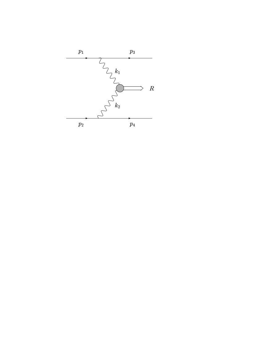
Figure 1: Kinematics for central production of a resonance

Recently it has been discovered that the pattern of resonances produced in the central region of double tagged $pp\rightarrow p+p+R$ depends on the vector difference of the transverse momentum recoil of the final state protons[1, 2] (even at fixed four-momentum transfers $t\sim-k_{1T}^{2},t^{\prime}\sim-k_{2T}^{2}$, see fig. 1 for kinematic definitions). When this quantity ($dk_{T}\equiv|\vec{k}_{T1}-\vec{k}_{T2}|$) is small, ($\leq O(\Lambda_{QCD})$), all well established $q\bar{q}$ states are observed to be suppressed while the surviving resonances include the enigmatic $f_{0}(1500),f_{J}(1710)$ which have been proposed as glueball candidates[3]. At large $dk_{T}$, by contrast, $q\bar{q}$ states are prominent, there appearing to be some correlation between their prominence and the internal angular momentum of their $q\bar{q}$ system such that high $L$ states turn on more with increasing $dk_{T}$ than do their low $L$ counterparts[4]. It has been suggested that this might form the basis of a glueball - $q\bar{q}$ filter since $0^{++},2^{++}$ glueballs need no internal angular momentum in contrast to the analogous $q\bar{q}$ ${}^{3}P_{0,2}$ combinations[1] and the dynamics may thereby favour glueballs as $dk_{T}\to 0$.

In order to gain insight, we have computed the production in a simple model where high energy $pp$ interactions are mediated by a preformed colour singlet object that couples to the proton $\sim\gamma_{\mu}$[5]. We find that when the resonance, $R$, has $J^{PC}=1^{++}$, $0^{-+}$ or $2^{-+}$ the predicted $dk_{T}$ dependence appears to be identical to that empirically observed in $pp\rightarrow p+p+R$ implying that central production of resonances is mediated by conserved vector currents independent of the nature of the meson, $R$. In contrast, we find that for $J^{PC}=(0,2)^{++}$ the structure of $R$ can be important enabling in principle a filtering of $q\bar{q}$ from glueballs to be realisable.

To be explicit, we shall calculate the production rate and momentum dependences of $\sigma(e^{+}(p_{1})e^{-}(p_{2})\rightarrow e^{+}(p_{3})+e^{-}(p_{4})+R)$ as this is well defined in QED and shares topological similarities to the hadronic processes of interest. First we shall generalise Cahn’s analysis of single tagged $e^{+}e^{-}$ [6] ($\gamma^{*}\gamma\to R$) to the double tagged case ($\gamma^{*}\gamma^{*}\to R$) for a general $1^{++}$ state. We define the production amplitude

$${\cal M}=e^{2}\bar{u}(p_{3})\not{\epsilon^{*}}u(p_{1})\bar{u}(p_{4})\not{\epsilon^{\prime*}}u(p_{2})\frac{1}{k_{1}^{2}k_{2}^{2}}\epsilon_{\mu}T^{\mu\nu}\epsilon^{\prime}_{\nu}$$ (1)

where for $1^{++}$ production the $\epsilon_{\mu}T^{\mu\nu}\epsilon^{\prime}_{\nu}$ may be written[7, 8] (with $k_{1}\equiv p_{1}-p_{3}$ and $k_{2}\equiv p_{2}-p_{4}$)

$$\epsilon_{\mu}T^{\mu\nu}\epsilon^{\prime}_{\nu}[1^{++}]= A_{1}(k_{1};k_{2})\epsilon_{\mu\nu\alpha\beta}\xi^{\beta}(G_{1}^{\mu\nu}G_{2}^{\alpha\delta}k_{\delta 2}+G_{2}^{\mu\nu}G_{1}^{\alpha\delta}k_{\delta 1})$$ (2)

$$+A_{2}(k_{1};k_{2})\epsilon_{\mu\nu\alpha\beta}\xi_{\delta}(k_{1}^{\delta}-k_{2}^{\delta})G_{1}^{\mu\nu}G_{2}^{\alpha\beta}$$

where we use the shorthand $G_{\mu\nu}\leftrightarrow k_{\mu}\epsilon_{\nu}-\epsilon_{\mu}k_{\nu}$ and the convention that $G_{1(2)}$ refers to $k_{1(2)},\epsilon_{1(2)}$; the $A_{i}(k_{1};k_{2})$ are form factors to be determined experimentally and $\xi$ is the spin polarisation vector for the axial meson.

For the special case of non-relativistic ${}^{3}P_{1}Q\bar{Q}$ one has[7, 8] $A_{2}\equiv 0$. It is straightforward to verify that the tensors multiplying $A_{1}$ may be written $\equiv\epsilon_{\mu\nu\alpha\beta}\xi^{\beta}\epsilon(1)^{\nu}\epsilon(2)^{\alpha}(k_{1}^{2}k_{2}^{\mu}-k_{2}^{2}k_{1}^{\mu})$ as in Cahn’s eqn(A1). In this case the double tagged differential cross section is

$$\frac{d\sigma}{dxdydtdt^{\prime}d\phi}\equiv\frac{e^{2}}{512\pi^{4}s}\frac{|A_{1}(t,t^{\prime})|^{2}}{t^{2}t^{\prime 2}}\delta(m^{2}+P_{T}^{2}-xys-(x+y)(t+t^{\prime}))|M|^{2}$$ (3)

where

$$|M|^{2}\equiv 2tt^{\prime}[t^{\prime}(su+s^{\prime}u^{\prime})+t(su^{\prime}+s^{\prime}u)-2cos\phi\sqrt{tt^{\prime}uu^{\prime}}(s+s^{\prime}-\frac{m^{2}}{2})]$$

$$+\frac{(t+t^{\prime})^{2}}{2m^{2}}[8uu^{\prime}tt^{\prime}sin^{2}\phi+(s-s^{\prime})^{2}+(u-u^{\prime})^{2}]$$ (4)

which reduces to Cahn’s eqns (A18,19,23) as $t\rightarrow 0$. Here $s,t,u$ are standard and $s^{\prime}=2p_{3}\cdot p_{4};t^{\prime}=-2p_{2}\cdot p_{4};u^{\prime}=-2p_{2}\cdot p_{3}$ which are related to the mass $m$ of the resonance by $s+s^{\prime}+t+t^{\prime}+u+u^{\prime}=m^{2}$ and$P_{T}$ is the recoil transverse momentum of the produced resonance. Furthermore we define $cos\phi\equiv\hat{p}_{3T}\cdot\hat{p}_{4T}$ when $p_{1,2}$ are aligned along the $\hat{z}$ axis; (note for future reference that the $dk_{T}$ phenomenon observed in $pp\rightarrow p+p+R$ is equivalent to a $\phi$ dependence of the cross section). We can make contact with the formalism used in ref[1] by defining $x,y$ as the fractional energy loss of the beams such that $p_{3}^{z}\approx(1-x)p_{1}^{z},p_{4}^{z}\approx(1-y)p_{2}^{z}$. Then eqn. S0.Ex2 may be written in the symmetric form

$$\frac{|M|^{2}}{-2tt^{\prime}s^{2}}=$$ (5)

$$t^{\prime}(1-y)[1+(1-x)^{2}]+t(1-x)[1+(1-y)^{2}]$$

$$+2cos\phi\sqrt{tt^{\prime}(1-x)(1-y)}[1+(1-x)(1-y)-\frac{xy}{2}]$$

$$-\frac{(t+t^{\prime})^{2}}{4m^{2}}([1+(1-y)^{2}][1+(1-x)^{2}]-4(1-x)(1-y)cos2\phi)$$

Consider now the particular limit, analogous to that in the $pp$ process, $t,t^{\prime}<<m^{2}$. Writing $t(1-x)=-k_{T1}^{2}$ and $t^{\prime}(1-y)=-k_{T2}^{2}$ and then taking the limit $x,y\rightarrow 0(\frac{1}{\sqrt{s}})$, eqn5 collapses to

$$|M|^{2}=4tt^{\prime}s^{2}\times[|\vec{k}_{T1}-\vec{k}_{T2}|^{2}]\equiv 4tt^{\prime}s^{2}|dk_{T}|^{2}.$$

Hence as $dk_{T}\rightarrow 0$ we predict that

$$Lim(dk_{T}\rightarrow 0)\frac{d\sigma}{dk_{T}}(e^{+}e^{-}\rightarrow e^{+}(k_{T1})e^{-}(k_{T2})R)\rightarrow 0.$$ (6)

We note that this is the same phenomenon observed in the $pp$ analogue[1, 2].

We find also that the $1^{++}$ should be spin polarised in the $\gamma^{*}\gamma^{*}$ c.m. frame. Following the approach of ref.[9] we predict

$$\frac{\sigma(\lambda=0)}{\sigma(\lambda=\pm 1)}=\frac{2(t-t^{\prime})^{2}}{(t+t^{\prime})m^{2}-2tt^{\prime}}$$ (7)

such that when $t,t^{\prime}<<m^{2}$ the $1^{++}$ $Q\bar{Q}$ will be produced dominantly with $\lambda=\pm 1$. Here again, the phenomenon predicted for $e^{+}e^{-}$ is apparently manifested empirically in $pp\rightarrow ppR$[4, 10], suggesting that the production is driven by conserved vector currents.

The suppression of $1^{++}$ as $dk_{T}\rightarrow 0$ is more general than for the specific $Q\bar{Q}$ case considered above. Inspection of the general amplitude, eqn (2), shows that the tensor multiplying $A_{2}$ vanishes as $k_{1T}-k_{2T}\rightarrow 0$. The production rate therefore also vanishes even when $A_{2}(k_{1};k_{2})\neq 0$ (assuming there is no pathological singularity in the $A_{2}$ form factor). Hence vanishing of axial meson production in this kinematic configuration is general for any production mechanism driven by conserved vector currents.

The similarity in behaviour between that observed in $pp\rightarrow p+p+R$ and that predicted in the analogous $e^{+}e^{-}$ arises for $R\equiv 0^{-+}$ too. As noted by Castodi and Frère [11] the production of $0^{-+}$ will naturally vanish as $dk_{T}\to 0$ if it is due to conserved vector current exchanges since in this case the production amplitude is proportional to

$$\epsilon_{\mu}T^{\mu\nu}\epsilon^{\prime}_{\nu}[0^{-+}]\equiv P(k_{1};k_{2})\epsilon^{\mu\nu\alpha\beta}G_{\mu\nu}G_{\alpha\beta}$$ (8)

which may be rewritten, in the meson rest frame,as $2MP(k_{1},k_{2})\epsilon_{ijk}(k_{1}-k_{2})_{i}\epsilon(1)_{j}\epsilon(2)_{k}$. Hence in the absence of a singular form factor this will vanish as $k_{1T}-k_{2T}\rightarrow 0$. The data of ref[2, 4] exhibit such a behaviour in $pp\rightarrow pp+\eta(\eta^{\prime})$. For non-relativistic $Q\bar{Q}$ spin singlets, ($0^{-+},2^{-+}$etc), where the production amplitude is proportional to derivatives of the wavefunction, the above structure (eq.8) will be generic (e.g. $2^{-+}$ in ref.[12]). Hence this sequence should disappear as $k_{1T}-k_{2T}\rightarrow 0$. This also is found to be true empirically for the $\eta_{2}(1620)$ and $\eta_{2}(1875)$ in $pp\rightarrow pp+\eta_{2}$[4, 13].

¿From the above analysis we infer that the $dk_{T}\rightarrow 0$ suppression for $0^{-+}$, $2^{-+}$ and $1^{++}$ production and the polarisation of the $1^{++}$ will all arise if the initiating fields are conserved vector currents. Thus they will naturally occur in $pp\rightarrow ppR$ if the resonance production is driven by conserved vectors, e.g. if the pomeron acts as a single hard gluon with colour neutralisation even at small $t$ (comapre and contrast ref[14]) and that production of $q\bar{q}$ is via gluon - gluon fusion. This is suggestive though not a proof. However, it can already be concluded from the WA102 phenomenon (refs.[1, 2]) that the pomeron must have a non-trivial helicity structure in order to generate non-trivial $\phi$ dependence[15]. Thus the Pomeron cannot be simply a scalar or pseudoscalar, in contrast to some outdated folklore, nor can it transform as simply the longitudinal component of a (non- conserved) vector[15, 16]. The implications of the Donnachie-Landshoff pomeron for $\phi$ dependence in central production merit study as do the general implications of $\phi$ dependence for the spin content of the Pomeron.

For the particular case of $gg$ fusion, or for $\gamma\gamma$ production, we may generalise the above analyses to $0^{++}$ and $2^{++}$ following refs.[7, 8, 17].

A linearly independent set of Lorentz and gauge invariant production amplitudes for $J^{++}$ states is given in [8, 17].The forms for $0^{-+}$ and $1^{++}$ in eqns.2 and 8 are as defined in ref.[8, 7]. The $0^{++}$ and $2^{++}$ cases are written

$$\epsilon_{\mu}T^{\mu\nu}\epsilon^{\prime}_{\nu}[0^{++}] = \frac{P_{\rho\sigma}}{\sqrt{3}}\left[S_{1}(k_{1},k_{2})G_{\mu\rho}^{1}G_{\nu\sigma}^{2}+S_{2}(k_{1},k_{2})k_{1}^{\mu}G^{1}_{\mu\rho}G^{2}_{\nu\sigma}k_{2}^{\nu}\right],$$ (9)

$$\epsilon_{\mu}T^{\mu\nu}\epsilon^{\prime}_{\nu}[2^{++}] = \epsilon_{\rho\sigma}\left[T_{1}(k_{1},k_{2})G^{1}_{\mu\rho}G^{2}_{\mu\sigma}+T_{2}(k_{1},k_{2})k_{1}^{\rho}k_{2}^{\sigma}G_{\mu\nu}^{1}G_{\mu\nu}^{2}\right.+$$ (10)

$$T_{3}(k_{1},k_{2})k_{1}^{\mu}G^{1}_{\mu\rho}G^{2}_{\nu\sigma}k_{2}^{\nu}\left.+T_{4}(k_{1},k_{2})k_{1}^{\rho}k_{2}^{\sigma}k_{1}^{\mu}G^{1}_{\mu\rho}G^{2}_{\nu\rho}k_{2}^{\nu}\right],$$

where

$$P_{\rho\sigma}\equiv g_{\rho\sigma}-\frac{P_{\rho}P_{\sigma}}{m^{2}},$$ (11)

for a resonance with mass $m$ and momentum $P_{\mu}$. Here $\epsilon_{\rho\sigma}$ is the polarization tensor satisfying

$$\sum_{\epsilon}\epsilon_{\rho\sigma}\epsilon_{\rho^{\prime}\sigma^{\prime}} = \frac{1}{2}(P_{\rho\rho^{\prime}}P_{\sigma\sigma^{\prime}}+P_{\rho\sigma^{\prime}}P_{\sigma\rho^{\prime}})-\frac{1}{3}P_{\rho\sigma}P_{\rho^{\prime}\sigma^{\prime}}.$$ (12)

The number of form factors reflects the number of independent helicity amplitudes for the $\gamma\gamma$ where, for transverse (T) or longitudinally polarised (L) photons one forms

$$0^{++}:\lambda=0;TTorLL$$

$$0^{-+}:\lambda=0;TT$$

$$1^{++}:\lambda=0;TT:\lambda=\pm 1;TL$$

$$2^{++}:\lambda=0;TT,LL:\lambda=\pm 1;TL:\lambda=\pm 2;TT.$$ (13)

The functional forms of the $F_{i}(k_{1},k_{2})$ depend on the composition of $R$. In the particular case where the form factor is modelled[18, 19, 8] as a QCD analogue[20] of the two photon coupling to positronium[21], the various $F_{1}\neq 0$ while $F_{2,3,4}=0$: this has been discussed in ref[7]. In this case there arise specific relations among the helicity amplitudes which is the source of the polarisation for the $1^{++}$ in eq.7. In the NRQM approximation[8]

$$\epsilon_{\mu}T^{\mu\nu}\epsilon^{\prime}_{\nu}[0^{++}(q\bar{q})]=c^{\prime}\sqrt{\frac{1}{6}}\left[G_{\mu\nu}^{a}G_{\mu\nu}^{a}(m^{2}+k_{1}\cdot k_{2})-2k_{1}^{\nu}G_{\mu\nu}^{a}G_{\mu\rho}^{a}k_{2}^{\rho}\right]/(k_{1}\cdot k_{2})^{2},$$ (14)

$$\equiv c^{\prime}m^{2}\sqrt{\frac{2}{3}}G_{\alpha\mu}^{1a}G_{\alpha\nu}^{2a}P_{\mu\nu}/(k_{1}\cdot k_{2})^{2},$$ (15)

and

$$\epsilon_{\mu}T^{\mu\nu}\epsilon^{\prime}_{\nu}[2^{++}(q\bar{q})]=c^{\prime}\sqrt{2}m^{2}G_{\mu\rho}^{a}G_{\nu\rho}^{a}e^{\mu\nu}/(k_{1}\cdot k_{2})^{2},$$ (16)

where the constants $c^{\prime}$ are proportional to the derivative of the radial wavefunctions at the origin:

$$c^{\prime}=g_{s}^{2}\sqrt{\frac{1}{m^{3}\pi}}R^{\prime}(0).$$ (17)

This structure implies that $2^{++}$ ${}^{3}P_{2}$ $q\bar{q}$ will be produced polarised with the $\lambda=0$ in the sense of eqns.(7 and S0.Ex8) suppressed at$O(tt^{\prime}/m^{2})$. This selection rule is expected to be realised even in the more physically relevant limit of light quarks[9].

The form factor for $0^{++}$ and $2^{++}$ glueballs in ref.[22] can be considered a natural relativistic generalization of TE mode glueballs in a cavity approximation such as the MIT bag model and the production amplitude takes the form[7]

$$\epsilon_{\mu}T^{\mu\nu}\epsilon^{\prime}_{\nu}[J^{++}(G)]={\cal P^{(J)}}_{\mu\nu}\frac{G^{1a}_{\mu\rho}G^{2a}_{\nu\rho}}{k_{1}\cdot k_{2}}F(k_{1};k_{2})$$ (18)

where ${\cal P^{(0)}}_{\mu\nu}\equiv P_{\mu\nu}/\sqrt{3}$ and ${\cal P^{(2)}}_{\mu\nu}\equiv\epsilon_{\mu\nu}$. The form factor $F(k_{1};k_{2})$ is determined by the glueball radial wavefunction common to the $0^{++}$ and $2^{++}$ states, so that the relative magnitudes of their form factors are fixed and the ensuing $dk_{T}$ dependences will be similar. The behaviour of $0^{++}$ and $2^{++}$ $q\bar{q}$ also will be similar to one another but in general will differ from those of the glueballs. We shall not speculate here on particular models for such form factors but address some general features.

For $(0,2)^{++}$ in general,any difference in the glueball and $q\bar{q}$ production will be driven by the form factors which are functions of two variables. The large momentum transfer behaviour of $P-wave$ $q\bar{q}$ and $S-wave$ glueballs with $J^{PC}=(0,2)^{++}$ may be constrained by power counting arguments[7, 23]. When $R$ is an $L=0$ bound state of two constituents, the leading large $k_{1}\cdot k_{2}$ behaviour of $F_{1}(k_{1};k_{2})$ is $\frac{1}{(k_{1}\cdot k_{2})}f(z)$ (where $z\equiv\frac{(k_{1}-k_{2})\cdot(k_{1}+k_{2})}{k_{1}\cdot k_{2}}$). The $F_{i}(k_{1};k_{2})$ entering the production amplitudes with additional factors of $k_{1,2}^{\mu}$ have correspondingly more rapid falloff. For $L=1$ systems at large $k_{1}\cdot k_{2}$ one expects an additional $\mu^{2}/k_{1}\cdot k_{2}$ suppression, where $\mu$ is a scale reflecting the variation of the wavefunction at the origin.

The behaviour of the $L=0$ and $L=1$ wavefunctions will also be expected to differ in general as their internal relative momenta $dp_{T}\to 0$. A suggestive model is if $dk_{T}$ correlates with the internal momentum $dp_{T}$ such that in the $L$-th partial wave

$$F(k_{1};k_{2})\sim|dk_{T}|^{L}\times\psi(t_{1};t_{2})$$

In such a situation as $|dk_{T}|\rightarrow 0$, ${}^{3}P_{0,2}$ $q\bar{q}$ states will be killed while $0^{+},2^{+}$ states controlled by $S$-waves (such as glueballs or strong coupling to pairs of $0^{-}$ mesons in S-wave) would survive. It is an open question whether the $dk_{T}\neq 0$ of the production mechanism is transferred into the relative momentum of the composite meson’s wavefunction. In the NRQM of eqns.(14-17) this does not occur; in the $t$-channel of $gg\to q\bar{q}$ where $(k_{1}-k_{2})^{2}\leq m_{q}^{2}$, the massive quark propagator that is implicit in the derivation of eqn.17 dilutes any such correlation. However, in the light quark limit there is the possibility for the singular behaviour of non-perturbative propagators[24] to cause a strong correlation between $dk_{T}$ and the internal (angular) momentum. This may be tested by measuring the $dk_{T}\to 0$ dependence of $0^{++},2^{++},4^{++}$ in $e^{+}e^{-}\to e^{+}e^{-}R$ and test if the $|dk_{T}|$ transmits to the wavefunction giving a $|dk_{T}|^{L}$ dependence. Our suggested strategy is as follows.

The similarity between the observed properties of $0^{-+}$ $2^{-+}$ and $1^{++}$ production in $pp\rightarrow ppR$ and those calculated for $e^{+}e^{-}\rightarrow e^{+}e^{-}R$ suggest that either diffractive scattering is driven by a colour singlet state transforming as a conserved vector current or/and that $gg\rightarrow R$ is the elemental process in the pomeron-pomeron interaction. This needs to be tested quantitatively. If verified, we may extend the concept of “stickiness”[25]. The recommended strategy is to measure $F^{R}_{\gamma\gamma}(k_{1};k_{2})$ in $e^{+}e^{-}\rightarrow e^{+}e^{-}R$ and compare with the analogous $F^{R}_{gg(?)}(k_{1};k_{2})$ in $pp\rightarrow ppR$. Observation of an identical $k_{1},k_{2}$ dependence in $pp\to ppR$ for the production of established $q\bar{q}$ states, such as $f_{2}(1270)$, would establish the conserved vector current dynamics of the double-pomeron production process. Conversely, the appearance of prominent states in $pp\rightarrow ppR$ that are suppressed in $e^{+}e^{-}\rightarrow e^{+}e^{-}R$ (“sticky” states[25]) and thereby are glueball candidates, would enable extraction of their $F_{i}(k_{1};k_{2})$. Such information would enable comparison of the production of $q\bar{q}$ states and the enigmatic states, thereby untangling their structure and dynamics.

Our general conclusions are as follows.

(i) The observed suppression of $0^{-+}$,$2^{-+}$ and $1^{++}$ as $dk_{T}\rightarrow 0$, and also polarisation of the $1^{++}$ will arise if the production mechanism involves conserved vector currents.

(ii) The production of $0^{++},2^{++}$ is richer. In these cases it will be the dynamical behaviour of the form factors $F_{i}(k_{1};k_{2})$, and hence the internal dynamics of the resonance $R$, that will determine the outcome. Thus there exists the possibility that $q\bar{q}$ and glueball states may be distinguishable in the $0^{++},2^{++}$ sectors. It is already clear that not all states of a given $J^{PC}$ behave the same; the established $q\bar{q}$ ${}^{3}P_{2}$ $f_{2}(1270;1525)$ disappear as $dk_{T}\rightarrow 0$ whereas $f_{2}(1930)$ survives[2, 4]. To investigate the source of this it is necessary to measure the various $F_{i}(k_{1};k_{2})$ and to compare $F_{(\gamma\gamma)}(k_{1};k_{2})$ with $F_{gg(?)}(k_{1};k_{2})$.

I am indebted to R.Cahn, M.Diehl, A.Donnachie, G.Farrar, J.Forshaw, J.-M.Frère, P.V.Landshoff and R.G.Roberts for discussions and comments and to A.Kirk and G.Gutierrez for information about their data.

References

• [1] F.E.Close and A.Kirk Phys Lett B 397 333 (1997)
• [2] WA102 Collaboration, Phys Lett B 397 339 (1997)
• [3] F E Close and C.Amsler, Phys Lett B 353 385 (1995); Phys Rev D 53 295 (1996)
D Weingarten, Proc of Lattice97, Proceedings of the International Symposium, Edinburgh,edited by C Davies et al
• [4] A.Kirk, Proc of Hadron97, Brookhaven, ed S.U.Chung et al
• [5] P.V.Landshoff and J.C.Polkinghorne, Nucl Phys B32 541 (1971)
P.V.Landshoff p323 in β€œDeep Inelastic Scattering and Related Phenomena”, ed G D’Agostini and A.Nigro (WOrld Scientific 1997)
• [6] R.Cahn, Phys Rev. D 35, 3342 (1987)
• [7] F.E.Close, G.Farrar and Z.P.Li, Phys Rev D55, 5749 (1997)
• [8] J. H. KΓΌhn, J. Kaplan, and E. Safiani, Nucl. Phys. 157, 125(1979).
• [9] Z.P.Li, F.E.Close and T.Barnes, Phys Rev D43,2161 (1991)
• [10] G.Gutierrez, Proc of Hadron97, Brookhaven, edited by S.U.Chung et al
• [11] P.Castodi and J.-M.FrΓ¨re, ULB report (unpublished)
J.-M.Frère, private communication.
• [12] J.Anderson, M.Austern and R.N.Cahn Phys Rev D43 2094 (1991)
• [13] WA102 Collaboration, hep-ph/9707021, Phys Letters (in press)
• [14] W.Buchmuller and A.Hebecker, Phys Lett B 355 573 (1995)
A.Edin, G. Ingelman and J.Rathsman, Phys Lett B 366 371 (1996)
A.White hep-ph/9709233
• [15] T.Arens,O.Nachtmann,M.Diehl and P.V.Landshoff Z.Phys C 74 651 (1997)
• [16] A.Donnachie and P.V.Landshoff, Nucl Phys B 244 322 (1984); ibid 267 690 (1986); Phys Lett B 185 403 (1987)
• [17] Y.Lepetre and F.M.Renard Nuovo Cimento Lett 5 117 (1972)
• [18] J. G. KΓΆrner, J.H.KΓΌhn, M. Krammer, and H. Schneider, Nucl. Phys. B229, 115(1983), J. G. KΓΆrner, J. H. KΓΌhn, and H. Schneider, Phys. Lett. 120B, 444(1983).
• [19] K. Koller and T. Walsh, Nucl. Phys. B140, 449 (1978).
• [20] R. Barbieri, R. Gatto, and R. Kogerler, Phys. Lett. 60B, 183(1976).
• [21] A. I. Alekseev, Zh. Eksp. Teor. Fiz. 34, 1195(1958)[Sov. Phys. JETP, 7, 826(1958)].
• [22] V.A.Novikov et al Nucl.Phys B191 301 (1981)
• [23] S.J.Brodsky and G.Farrar, Phys Rev Letters 31 1153 (1973)
• [24] M.R.Pennington (private communication)
N.Brown and M.R.Pennington Phys.Rev D38 2266 (1988)
• [25] M.Chanowitz, Proc of 6th International Workshop on Photon-Photon Collisions, Lake Tahoe, 1984, edited by R.Lander (World Scientific, 1985)
Refer to caption