Abstract

In the supersymmetric extension of the Standard Model we derive the two–loop QCD corrections to the scalar quark contributions to the electroweak precision observables entering via the $\rho$ parameter. A very compact expression is derived for the gluon–exchange contribution. The complete analytic result for the gluino–exchange contribution is very lengthy; we give expressions for several limiting cases that were derived from the general result. The two–loop corrections, generally of the order of 10 to 30% of the one-loop contributions, can be very significant. Contrary to the Standard Model case, where the QCD corrections are negative and screen the one–loop value, the corresponding corrections in the supersymmetric case are in general positive, therefore increasing the sensitivity in the search for scalar quarks through their virtual effects in high–precision electroweak observables.

1. Introduction

Supersymmetric theories (SUSY) [1] are widely considered as the theoretically most appealing extension of the Standard Model (SM). They are consistent with the approximate unification of the three gauge coupling constants at the GUT scale and provide a way to cancel the quadratic divergences in the Higgs sector hence stabilizing the huge hierarchy between the GUT and the Fermi scales. Furthermore, in SUSY theories the breaking of the electroweak symmetry is naturally induced at the Fermi scale, and the lightest supersymmetric particle can be neutral, weakly interacting and absolutely stable, providing therefore a natural solution for the Dark Matter problem; for recent reviews see for instance Ref. [2].

Supersymmetry predicts the existence of scalar partners $\tilde{f}_{L},\tilde{f}_{R}$ to each SM chiral fermion, and spin–1/2 partners to the gauge bosons and to the scalar Higgs bosons. So far, the direct search of SUSY particles at present colliders has not been successful. One can only set lower bounds of ${\cal O}(100)$ GeV on their masses [3]. The search for SUSY particles can be extended to slightly larger values in the next runs at LEP2 and at the upgraded Tevatron. To sweep the entire mass range for the SUSY particles, which from naturalness arguments is expected not to be larger than the TeV scale, the higher energy hadron or $e^{+}e^{-}$ colliders of the next decade will be required.

An alternative way to probe SUSY is to search for the virtual effects of the additional particles. Indeed, now that the top–quark mass is known [4], and its measured value is in remarkable agreement with the one indirectly obtained from high–precision electroweak data, one can use the available data to search for the quantum effects of the SUSY particles: sleptons, squarks, gluinos and charginos/neutralinos. In the Minimal Supersymmetric Standard Model (MSSM) there are three main possibilities for the virtual effects of SUSY particles to be large enough to be detected in present experiments:

• In the rare decay $b\rightarrow s\gamma$, besides the SM top/W–boson loop contribution, one has additional contributions from chargino/stop and charged Higgs/stop loops [5]. These contributions can be sizable but the two new contributions can interfere destructively in large areas of the MSSM parameter space, leading in this case to a small correction to the decay rate predicted by the SM.

• If charginos and scalar top quarks are light enough, they can affect the partial decay width of the Z boson into $b$ quarks in a sizable way [6]. This feature has been widely discussed in the recent years, in view of the deviation of the $Z\rightarrow b\bar{b}$ partial width from the SM prediction [7]. However, for chargino and stop masses beyond the LEP2 or Tevatron reach, these effects become too small to be observable [7].

• A third possibility is the contribution of the scalar quark loops, in particular stop and sbottom loops, to the electroweak gauge–boson self–energies [8, 9]: if there is a large splitting between the masses of these particles, the contribution will grow with the square of the mass of the heaviest scalar quark and can be very large. This is similar to the SM case where the top/bottom weak isodoublet generates a quantum correction that grows as the top–quark mass squared.

In this paper, we will focus on the third possibility and discuss in detail the leading contribution of scalar quark loops to electroweak precision observables, which is parameterized by their contribution to the $\rho$ parameter. The radiative corrections affecting the vector boson self–energies stemming from charginos, neutralinos and Higgs bosons have been discussed in several papers [8, 9]. In the MSSM, because of the strong constraints on the Higgs sector, the propagator corrections due to Higgs particles are very close to those of the SM for a light Higgs boson [10]. In the decoupling regime where all scalar Higgs bosons but the lightest are very heavy, the SUSY Higgs sector is effectively equivalent to the SM Higgs sector with a Higgs–boson mass of the order of 100 GeV. The contribution of charginos and neutralinos, except from threshold effects, is also very small [9]. The main reason is that the custodial symmetry which guarantees that $\rho=1$ at the tree level is only weakly broken in this sector since the terms which can break this symmetry in the chargino/neutralino mass matrices are all proportional to $M_{W}$ and hence bounded in magnitude [9].

The propagator corrections from squark loops to the electroweak observables can be attributed, to a large extent, to the correction to the $\rho$ parameter [11], which measures the relative strength of the neutral to charged current processes at zero momentum–transfer. This is similar to the SM, where the top/bottom contribution to the precision observables is, to a very good approximation, proportional to their contribution to the deviation of the $\rho$ parameter from unity. Further contributions, compared to the previous one, are suppressed by powers of the heavy masses. It is mainly from this contribution that the top–quark mass has been successfully predicted from the measurement of the Z–boson observables and of the W–boson mass at hadron colliders. However, in order for the predicted value to agree with the experimental one, higher–order radiative corrections [12, 13, 14] had to be included. For instance, the two–loop QCD corrections lead to a decrease of the one–loop result by approximately $10\%$ and shift the top–quark mass upwards by an amount of $\sim 10$ GeV.

In order to treat the SUSY loop contributions to the electroweak observables at the same level of accuracy as the standard contribution, higher–order corrections should be incorporated. In particular the QCD corrections, which because of the large value of the strong coupling constant can be rather important, must be known. In a short letter [15] we have recently presented the results for the ${\cal O}(\alpha_{s})$ correction to the contribution of the scalar top and bottom quark loops to the $\rho$ parameter. In this article we give the main details of the calculation and present the explicit result for the gluon–exchange contribution as well as the result for the gluino–exchange contribution in several limiting cases.

The paper is organized as follows. In the next section, we summarize the one–loop results and fix the notation. The main features of the two–loop calculation are discussed in section 3. In section 4 a compact expression is given for the gluon–exchange contributions. The results for the gluino–exchange contributions are presented for the limiting cases of zero gluino mass and a very heavy gluino as well as for the case of arbitrary gluino mass but vanishing squark mixing. Effects of ${\cal O}(\alpha_{s})$ corrections to relations between the squark masses existing in different scenarios are discussed. In section 5 we give our conclusions.

2. One-loop results

For the sake of completeness, we summarize in this section the one–loop contribution of a squark doublet to the electroweak precision observables. Before that, to set the notation, we first discuss the masses and couplings of scalar quarks in the MSSM.

As mentioned previously, SUSY associates a left– and a right–handed scalar partner to each SM quark. The current eigenstates, $\tilde{q}_{L}$ and $\tilde{q}_{R}$, mix to give the mass eigenstates $\tilde{q}_{1}$ and $\tilde{q}_{2}$; the mixing angle is proportional to the quark mass and is therefore important only in the case of the third generation squarks. In the MSSM, the squark masses are given in terms of the Higgs–higgsino mass parameter $\mu$, the ratio of the vacuum expectation values $\tan\beta$ of the two Higgs doublet MSSM fields needed to break the electroweak symmetry, the left– and right–handed scalar masses $M_{\tilde{q}_{L}}$ and $M_{\tilde{q}_{R}}$ and the soft–SUSY breaking trilinear coupling $A_{q}$. The top and bottom squark mass eigenstates and their mixing angles are determined by diagonalizing the following mass matrices

$${\cal M}^{2}_{\tilde{t}}=\left(\begin{array}[]{cc}M_{\tilde{t}_{L}}^{2}+m_{t}^{2}+\cos 2\beta(\frac{1}{2}-\frac{2}{3}s_{W}^{2})\,M_{Z}^{2}&m_{t}\,M^{LR}_{t}\\ m_{t}\,M^{LR}_{t}&M_{\tilde{t}_{R}}^{2}+m_{t}^{2}+\frac{2}{3}\cos 2\beta\;s_{W}^{2}\,M_{Z}^{2}\end{array}\right)$$ (1)

$${\cal M}^{2}_{\tilde{b}}=\left(\begin{array}[]{cc}M_{\tilde{b}_{L}}^{2}+m_{b}^{2}+\cos 2\beta(-\frac{1}{2}+\frac{1}{3}s_{W}^{2})\,M_{Z}^{2}&m_{b}\,M^{LR}_{b}\\ m_{b}\,M^{LR}_{b}&M_{\tilde{b}_{R}}^{2}+m_{b}^{2}-\frac{1}{3}\cos 2\beta\;s_{W}^{2}\,M_{Z}^{2}\end{array}\right),$$ (2)

with $M^{LR}_{t}=A_{t}-\mu\,\cot\beta\hskip 2.84526pt$ and $M^{LR}_{b}=A_{b}-\mu\tan\beta\hskip 2.84526pt$; $s_{W}^{2}=1-c_{W}^{2}\equiv\sin^{2}\theta_{W}$. Furthermore, SU(2) gauge invariance requires $M_{\tilde{t}_{L}}=M_{\tilde{b}_{L}}$ at the tree–level. Expressed in terms of the squark masses $m_{\tilde{q}_{1}},m_{\tilde{q}_{2}}$ and the mixing angle $\theta_{\tilde{q}}$ the squark mass matrices read

$${\cal M}^{2}_{\tilde{q}}=\left(\begin{array}[]{cc}\cos^{2}\theta_{\tilde{q}}m^{2}_{\tilde{q}_{1}}+\sin^{2}\theta_{\tilde{q}}m^{2}_{\tilde{q}_{2}}&\sin\theta_{\tilde{q}}\cos\theta_{\tilde{q}}(m^{2}_{\tilde{q}_{1}}-m^{2}_{\tilde{q}_{2}})\\ \sin\theta_{\tilde{q}}\cos\theta_{\tilde{q}}(m^{2}_{\tilde{q}_{1}}-m^{2}_{\tilde{q}_{2}})&\sin^{2}\theta_{\tilde{q}}m^{2}_{\tilde{q}_{1}}+\cos^{2}\theta_{\tilde{q}}m^{2}_{\tilde{q}_{2}}\end{array}\right).$$ (3)

Due to the large value of the top–quark mass $m_{t}$, the mixing between the left– and right–handed top squarks $\tilde{t}_{L}$ and $\tilde{t}_{R}$ can be very large, and after diagonalization of the mass matrix the lightest scalar top–quark mass eigenstate $\tilde{t}_{1}$ can be much lighter than the top quark and all the scalar partners of the light quarks [16]. The mixing in the sbottom sector is in general rather small, except if $A_{b},\mu$ or $\tan\beta$ are extremely large. In most of our discussion we will assume that, because of the small bottom mass, the mixing in the sbottom sector is negligible and therefore $\tilde{b}_{L}\equiv\tilde{b}_{1}$.

Using the notation of the first generation, the contribution of a squark doublet $\tilde{u},\tilde{d}$ to the self–energy of a vector boson $V\equiv\gamma,Z,W$ and to the $Z$–$\gamma$ mixing is given by the diagrams of Fig. 1. Summing over all possible flavors and helicities, the squark contribution to the transverse parts of the gauge–boson self–energies at arbitrary momentum–transfer $q^{2}$ can be written, in terms of the Fermi constant $G_{F}$, as follows:

$$\Pi_{WW}(q^{2}) = -\frac{3G_{F}M_{W}^{2}}{8\sqrt{2}\pi^{2}}\sum_{i,j=1,2}g_{W\tilde{u}_{i}\tilde{d}_{j}}^{2}\,\Pi_{0}(q^{2},m_{\tilde{u}_{i}}^{2},m_{\tilde{d}_{j}}^{2})$$

$$\Pi_{ZZ}(q^{2}) = -\frac{3G_{F}M_{Z}^{2}}{4\sqrt{2}\pi^{2}}\sum_{\tilde{q}=\tilde{u},\tilde{d}\atop i,j=1,2}g_{Z\tilde{q}_{i}\tilde{q}_{j}}^{2}\,\Pi_{0}(q^{2},m_{\tilde{q}_{i}}^{2},m_{\tilde{q}_{j}}^{2})$$

$$\Pi_{Z\gamma}(q^{2}) = -\frac{3G_{F}M_{Z}^{2}s_{W}c_{W}}{4\sqrt{2}\pi^{2}}\sum_{\tilde{q}=\tilde{u},\tilde{d}\atop i=1,2}g_{Z\tilde{q}_{i}\tilde{q}_{j}}e_{\tilde{q}_{i}}\,\Pi_{0}(q^{2},m_{\tilde{q}_{i}}^{2},m_{\tilde{q}_{i}}^{2})$$

$$\Pi_{\gamma\gamma}(q^{2}) = -\frac{3G_{F}M_{Z}^{2}s_{W}^{2}c_{W}^{2}}{4\sqrt{2}\pi^{2}}\sum_{\tilde{q}=\tilde{u},\tilde{d}\atop i=1,2}e_{\tilde{q}_{i}}^{2}\,\Pi_{0}(q^{2},m_{\tilde{q}_{i}}^{2},m_{\tilde{q}_{i}}^{2}),$$ (4)

with the reduced couplings of the squarks to the $W$ and $Z$ bosons, including mixing $\theta_{\tilde{q}}$ between left– and right–handed squarks, given by ($e_{q}$ and $I_{3}^{q}$ are the electric charge and the weak isospin of the partner quark)

$$g_{W\tilde{u}_{i}\tilde{d}_{j}}=\left(\begin{array}[]{cc}\cos\theta_{\tilde{u}}\cos\theta_{\tilde{d}}&-\cos\theta_{\tilde{u}}\sin\theta_{\tilde{d}}\\ -\cos\theta_{\tilde{u}}\sin\theta_{\tilde{d}}&\sin\theta_{\tilde{u}}\sin\theta_{\tilde{d}}\end{array}\right),$$ (7)

$$g_{Z\tilde{q}_{i}\tilde{q}_{j}}=\left(\begin{array}[]{cc}(I^{q}_{3}-e_{q}s_{W}^{2})\cos^{2}\theta_{\tilde{q}}-e_{q}s_{W}^{2}\sin^{2}\theta_{\tilde{q}}&-I_{3}^{q}\sin\theta_{\tilde{q}}\cos\theta_{\tilde{q}}\\ -I_{3}^{q}\sin\theta_{\tilde{q}}\cos\theta_{\tilde{q}}&-e_{q}s_{W}^{2}\cos^{2}\theta_{\tilde{q}}+(I^{q}_{3}-e_{q}s_{W}^{2})\sin^{2}\theta_{\tilde{q}}\end{array}\right).$$ (10)

In both the dimensional regularization [17] and dimensional reduction [18] schemes, the function $\Pi_{0}(q^{2},m_{a}^{2},m_{b}^{2})$ reads

$$\Pi_{0}(q^{2},m_{a}^{2},m_{b}^{2})=\frac{4}{3}\left[m_{a}^{2}+m_{b}^{2}-\frac{q^{2}}{3}+\left(m_{a}^{2}+m_{b}^{2}-\frac{q^{2}}{2}-\frac{(m_{a}^{2}-m^{2}_{b})^{2}}{2\,q^{2}}\right)B_{0}(q^{2},m_{a},m_{b})\right.$$

$$\left.+\frac{m_{a}^{2}-m_{b}^{2}}{2\,q^{2}}(A_{0}(m_{a})-A_{0}(m_{b}))-A_{0}(m_{a})-A_{0}(m_{b})\right].$$ (11)

The Passarino–Veltman one– and two–point functions [19] are defined as

$$A_{0}(m) = m^{2}\left[\frac{1}{\epsilon}+1-\ln\frac{m^{2}}{\mu^{2}}+\epsilon\left(1+\frac{\pi^{2}}{12}-\ln\frac{m^{2}}{\mu^{2}}+\frac{1}{2}\,\ln^{2}\frac{m^{2}}{\mu^{2}}\right)\right]$$

$$B_{0}(q^{2},m_{a},m_{b}) = \frac{1}{\epsilon}+B_{0}^{\rm fin}(q^{2},m_{a},m_{b})+\epsilon\,B_{0}^{\epsilon}(q^{2},m_{a},m_{b})$$

$$B_{0}^{\rm fin}(q^{2},m_{a},m_{b}) = 2-\ln\frac{m_{a}m_{b}}{\mu^{2}}+\frac{m_{a}^{2}-m_{b}^{2}}{q^{2}}\ln\frac{m_{a}}{m_{b}}$$ (12)

$$+\frac{\beta^{1/2}(q^{2},m_{a}^{2},m_{b}^{2})}{q^{2}}\ln\frac{m_{a}^{2}+m_{b}^{2}-q^{2}+\beta^{1/2}(q^{2},m_{a}^{2},m_{b}^{2})}{2m_{a}m_{b}},$$

where $\mu$ is the renormalization scale, $\beta$ the phase space function,

$$\beta(q^{2},m_{a}^{2},m_{b}^{2})=q^{2}-m_{a}^{2}-m_{b}^{2}+\frac{(m_{a}^{2}-m_{b}^{2})^{2}}{q^{2}},$$ (13)

and $2\epsilon=4-n$ with $n$ the space–time dimension. We have absorbed a factor $(e^{\gamma}/4\pi)^{\epsilon}$, with $\gamma$ the Euler constant, in the ’t Hooft scale $\mu$ to prevent uninteresting combinations of $\ln 4\pi,\ \gamma\ldots$ in our results. The explicit form of the function $B_{0}^{\epsilon}$ is not needed for our purposes but can be found in Ref. [20].

At zero momentum–transfer, $q^{2}=0$, the function $\Pi_{0}$ is finite and reduces to

$$F_{0}(m_{a}^{2},m_{b}^{2})\equiv\Pi_{0}(0,m_{a}^{2},m_{b}^{2})=m_{a}^{2}+m_{b}^{2}-\frac{2m_{a}^{2}m_{b}^{2}}{m_{a}^{2}-m_{b}^{2}}\ln\frac{m_{a}^{2}}{m_{b}^{2}}.$$ (14)

We now focus on the contribution of a squark doublet to the $\rho$ parameter. It is well-known that the deviation of the $\rho$ parameter from unity parameterizes the leading universal corrections induced by heavy fields in electroweak amplitudes. It is due to a mass splitting between the fields in an isospin doublet. Compared to this correction all additional contributions are suppressed. In the relevant cases of the W–boson mass and of the effective weak mixing angle $\sin^{2}\theta_{W}^{\rm eff}$, for example, a doublet of heavy squarks would induce shifts proportional to its contribution to $\rho$,

$$\delta M_{W}\approx\frac{M_{W}}{2}\frac{c_{W}^{2}}{c_{W}^{2}-s_{W}^{2}}\Delta\rho;\ \ \ \ \delta\sin^{2}\theta_{W}^{\rm eff}\approx-\frac{c_{W}^{2}s_{W}^{2}}{c_{W}^{2}-s_{W}^{2}}\Delta\rho.$$ (15)

In terms of the transverse parts of the W– and Z–boson self–energies at zero momentum–transfer, the squark loop contribution to the $\rho$ parameter is given by

$$\rho=\frac{1}{1-\Delta\rho}\ ;\ \ \ \ \Delta\rho=\frac{\Pi_{ZZ}(0)}{M_{Z}^{2}}-\frac{\Pi_{WW}(0)}{M_{W}^{2}}\ .$$ (16)

Using the previous expressions for the W– and Z–boson self-energies and neglecting the mixing in the sbottom sector, one obtains for the contribution of the $\tilde{t}/\tilde{b}$ doublet at one–loop order (only the left–handed sbottom $\tilde{b}_{L}$ contributes for $\theta_{\tilde{b}}=0$) :

$$\Delta\rho_{0}^{\mathrm{S}USY} = \frac{3G_{F}}{8\sqrt{2}\pi^{2}}\left[-\sin^{2}\theta_{\tilde{t}}\cos^{2}\theta_{\tilde{t}}\ F_{0}(m_{\tilde{t}_{1}}^{2},m_{\tilde{t}_{2}}^{2})+\cos^{2}\theta_{\tilde{t}}\ F_{0}(m_{\tilde{t}_{1}}^{2},m_{\tilde{b}_{L}}^{2})\right.$$ (17)

$$\left.{}+\sin^{2}\theta_{\tilde{t}}\ F_{0}(m_{\tilde{t}_{2}}^{2},m_{\tilde{b}_{L}}^{2})\right].$$

The function $F_{0}$ vanishes when the two squarks running in the loop are degenerate in mass, $F_{0}(m_{q}^{2},m_{q}^{2})=0$. In the limit of large squark mass splitting it becomes proportional to the heavy squark mass squared: $F_{0}(m_{a}^{2},0)=m_{a}^{2}$. Therefore, the contribution of a squark doublet becomes in principle very large when the mass splitting between squarks is large. This is exactly the same situation as in the case of the SM where the top/bottom contribution to the $\rho$ parameter at one–loop order, keeping both the $t$ and $b$ quark masses, reads [11]

$$\Delta\rho_{0}^{\rm SM}=\frac{3G_{F}}{8\sqrt{2}\pi^{2}}F_{0}(m_{t}^{2},m_{b}^{2}).$$ (18)

For $m_{t}\gg m_{b}$ this leads to the well–known quadratic correction $\Delta\rho_{0}^{\rm SM}=3G_{F}m_{t}^{2}/(8\sqrt{2}\pi^{2})$.

In Fig. 2 we display the one–loop correction to the $\rho$ parameter that is induced by the $\tilde{t}/\tilde{b}$ isodoublet. The scalar mass parameters are assumed to be equal, $M_{\tilde{t}_{L}}=M_{\tilde{t}_{R}}$ and $M_{\tilde{b}_{L}}=M_{\tilde{b}_{R}}$, as it is approximately the case in Supergravity models with scalar mass unification at the GUT scale [21]. As mentioned above, SU(2) gauge invariance requires at the tree–level $M_{\tilde{t}_{L}}=M_{\tilde{b}_{L}}$, yielding in this case $M_{\tilde{t}_{L}}=M_{\tilde{t}_{R}}=M_{\tilde{b}_{L}}=M_{\tilde{b}_{R}}=m_{\tilde{q}}$. In this scenario, the scalar top mixing angle is either very small, $\theta_{\tilde{t}}\sim 0$, or almost maximal, $\theta_{\tilde{t}}\sim-\pi/4$, in most of the MSSM parameter space. The contribution $\Delta\rho_{0}^{\mathrm{S}USY}$ is shown as a function of the common squark mass $m_{\tilde{q}}$ for $\tan\beta=1.6$ for the two cases $M^{LR}_{t}=0$ (no mixing) and $M_{t}^{LR}=200$ GeV (maximal mixing); the bottom mass and therefore the mixing in the sbottom sector are neglected leading to $m_{\tilde{b}_{L}}=m_{\tilde{b}_{1}}\simeq m_{\tilde{q}}$. Here and in all the numerical calculations in this paper we use $m_{t}=175$ GeV, $M_{Z}=91.187$ GeV, $M_{W}=80.33$ GeV, and $\alpha_{s}=0.12$. The electroweak mixing angle is defined from the ratio of the vector boson masses: $s_{W}^{2}=1-M_{W}^{2}/M_{Z}^{2}$.

As can be seen, the correction is rather large for small $m_{\tilde{q}}$, exceeding the level $\Delta\rho=1.3\times 10^{-3}$ of experimental sensitivity in the case of no mixing for $m_{\tilde{q}}\sim 150$ GeV, which corresponds to the experimental lower bound on the common squark mass [3], and getting very close to it in the case of maximal mixing. For large $m_{\tilde{q}}$ values, the two stop and the sbottom masses are approximately degenerate since $m_{\tilde{q}}\gg m_{t}$, and the contribution to $\Delta\rho$ becomes very small.

For illustration, we have chosen the value $\tan\beta\hskip 2.84526pt=1.6$ which is favored by $b$–$\tau$ Yukawa coupling unification scenarios [21]. In fact, the analysis depends only marginally on $\tan\beta$ if $M^{LR}_{t}$ (and not $A_{t}$ and $\mu$) is used as input parameter. The only effect of varying $\tan\beta\hskip 2.84526pt$ is then to slightly alter the D–terms in the mass matrices eqs. (1–2), which does not change the situation in a significant way. However, for large $\tan\beta$ values, $\tan\beta\hskip 2.84526pt\sim m_{t}/m_{b}$, the mixing in the sbottom sector has to be taken into account, rendering the analysis somewhat more involved. We will focus on the scenario with a low value of $\tan\beta\hskip 2.84526pt$ in the following.

In Fig. 3 we display $\Delta\rho_{0}^{\mathrm{S}USY}$ as a function of the mixing angle for three values of the common squark mass, $m_{\tilde{q}}=150$, 250 and 500 GeV, and for $\tan\beta\hskip 2.84526pt=1.6$. The contribution is practically flat except for values of the mixing angle very close to the lower limit, $\theta_{\tilde{q}}\sim-\pi/4$. This justifies the choice of concentrating on the two extreme cases. In fact, in the case $M_{\tilde{t}_{L}}=M_{\tilde{t}_{R}}$, the maximal mixing scenario $\theta_{\tilde{q}}=-\pi/4$ is only obtained exactly when the D–terms are set to zero, which is the case when $\tan\beta=1$. One can also have maximal mixing if the sums of $M_{\tilde{t}_{L}}^{2}$ and $M_{\tilde{t}_{R}}^{2}$ with their corresponding D–terms are equal, making the diagonal entries in the mass matrices eqs. (1–2) identical.

The parameter $M_{t}^{LR}$ does not only influence the mixing but also the mass splitting between the scalar top quarks. The effect of varying $M_{t}^{LR}$ on $\Delta\rho_{0}^{\rm SUSY}$ is displayed in Table 1 for the case of exact maximal mixing, i.e. $\tan\beta\hskip 2.84526pt=1$. The scenario with $\tan\beta\hskip 2.84526pt=1.6$ yields similar numerical results. For large values of $M_{t}^{LR}$ the contribution to the $\rho$ parameter can become huge, exceeding by far the level of experimental observability. The increase of $\Delta\rho_{0}^{\rm SUSY}$ with larger values of $M_{t}^{LR}$ is due to the increased mass splitting between the two stop masses and $m_{\tilde{b}_{1}}$ that is induced for $m_{t}M_{t}^{LR}\gg m_{\tilde{q}}^{2}$. For values of $m_{\tilde{q}}$ comparable to the top quark mass, $m_{\tilde{q}}\raisebox{-3.69899pt}{~{}\shortstack{$<$ \\ [-0.07cm] $\sim$}}~{}200$ GeV, the mass splitting is already large even for small $M_{t}^{LR}$ due to the additional $m_{t}^{2}$ term in the stop mass matrix; this is similar to the no–mixing case.

If the GUT relation $M_{\tilde{t}_{L}}\simeq M_{\tilde{t}_{R}}$ is relaxed and large values of the mixing parameter $M_{t}^{LR}$ are assumed, the splitting between the stop and sbottom masses is so large that the contribution to the $\rho$ parameter can become even bigger than in the previously discussed scenario (see subsection 4.4 for a more detailed discussion).

$m_{\tilde{q}}$ (GeV)	$M_{t}^{LR}$ (GeV)	$\Delta\rho_{0}^{\rm SUSY}\times 10^{-3}$
200	100	1.68
	200	1.35
	300	0.89
	400	1.28
500	200	0.34
	500	0.23
	1400	2.04
	1550	4.97
800	500	0.12
	1500	0.07
	2000	0.30
	3700	15.8

Table 1: $\Delta\rho_{0}^{\rm SUSY}$ in units of $10^{-3}$ for several values of $m_{\tilde{q}}$ and $M_{t}^{LR}$ (in GeV) and $\tan\beta\hskip 2.84526pt=1$. The values of $M_{t}^{LR}$ are chosen such that the corresponding squark masses lie in the experimentally allowed range.

3. Two–loop calculation

3.1. Renormalization

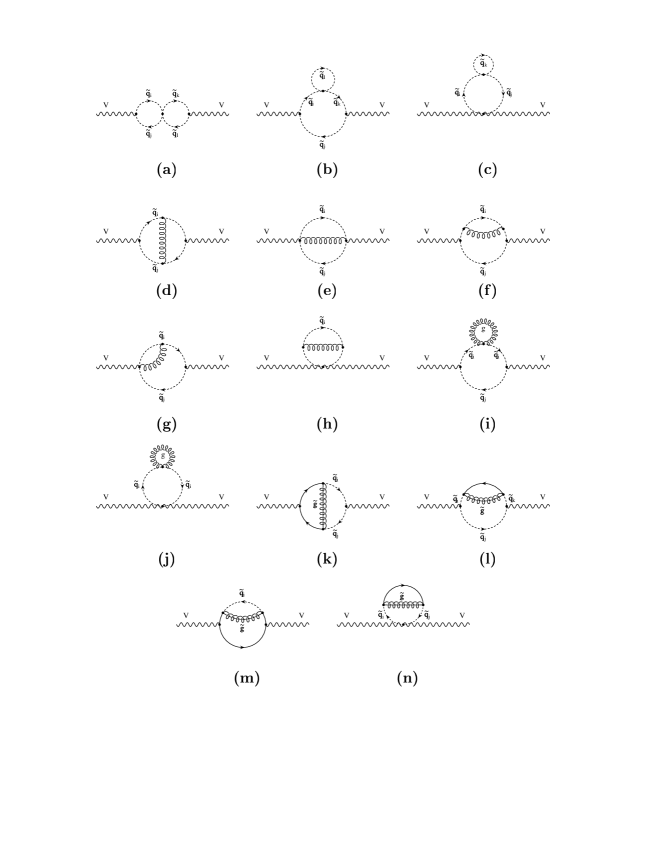
Figure 4: Feynman diagrams for the contribution of scalar quark loops to the gauge–boson self–energies at two–loop order.

The QCD corrections to the squark contributions to the vector boson self–energies, Fig. 4, can be divided into three different classes: the pure scalar diagrams (Fig. 4a–c), the gluon exchange diagrams (Fig. 4d–j), and the gluino–exchange diagrams (Fig. 4k–n). These diagrams have to be supplemented by counterterms for the squark and quark mass renormalization (Fig. 5a–c) as well as for the renormalization of the squark mixing angle, (Fig. 5d). The three different sets of contributions together with the respective counterterms are separately gauge–invariant and ultraviolet finite. For the gluon exchange contribution we have only considered the squark loops, since the gluon exchange in quark loops is just the SM contribution, yielding the result $\Delta\rho^{\rm SM}_{1}=-\Delta\rho_{0}^{\rm SM}\frac{2}{3}\frac{\alpha_{s}}{\pi}(1+\pi^{2}/3)$ [12].

As mentioned above, the results presented in the following are precisely the same in dimensional regularization as in dimensional reduction. The renormalization procedure is performed as follows. We work in the on–shell scheme where the quark and squark masses are defined as the real part of the pole of the corresponding propagators. One further needs a prescription for the renormalization of the squark mixing angle. The renormalized mixing angle can be defined by requiring that the renormalized squark mixing self–energy $\Pi_{\tilde{q}_{1}\tilde{q}_{2}}^{\rm ren}(q^{2})$ vanishes at a given momentum–transfer $q_{0}^{2}$, for example when one of the two squarks is on-shell. This means that the two squark mass eigenstates $\tilde{q_{1}}$ and $\tilde{q_{2}}$ do not mix but propagate independently for this value of $q^{2}$. Expressing the parameters in eq. (3) by renormalized quantities and choosing the field renormalization of the squarks appropriately, this renormalization condition yields for the mixing angle counterterm

$$\delta\theta_{\tilde{q}}(q_{0}^{2})=\frac{1}{m^{2}_{\tilde{q}_{1}}-m^{2}_{\tilde{q}_{2}}}\Pi_{\tilde{q}_{1}\tilde{q}_{2}}(q_{0}^{2}).$$ (19)

Finally, we have also included, as a check, the field renormalization constants of the quarks and the squarks in our calculation; they of course have to drop out in the final result, which we have verified by explicit calculation.

The one–loop diagrams of Fig. 6a–c provide the renormalization of the squark masses and the squark wave functions. As the one–loop squark contributions to the vector boson self-energies are finite at vanishing external momentum (see eq. (14)), we notice that the $O(\epsilon)$ part of the squark mass counterterm is not needed. We have contributions from the three diagrams of Fig. 6a, b, and c involving gluon exchange, gluino exchange and a pure scalar contribution, respectively. The explicit form of the pure scalar contribution is not needed as we will see later. The contribution of the gluon exchange to the squark mass counterterm is given by

$$m_{\tilde{q}_{i}}\delta^{g}m_{\tilde{q}_{i}}=-\,\frac{\alpha_{s}}{2\pi}\,m_{\tilde{q}_{i}}^{2}\left[\frac{1}{\epsilon}+\frac{7}{3}-\ln\frac{m_{\tilde{q}_{i}}^{2}}{\mu^{2}}\right],$$ (20)

while the one of the gluino exchange reads

$$m_{\tilde{q}_{i}}\delta^{\tilde{g}}m_{\tilde{q}_{i}} = -\,\frac{\alpha_{s}}{3\pi}\left[(m_{q}^{2}+m_{\tilde{g}}^{2}-m_{\tilde{q}_{i}}^{2})\;B_{0}(m_{\tilde{q}_{i}}^{2},m_{q},m_{\tilde{g}})+A_{0}(m_{\tilde{g}})+A_{0}(m_{q})\right.$$ (21)

$$+\left.2(-1)^{i}\sin 2\theta_{\tilde{q}}\;m_{\tilde{g}}\,m_{q}\;B_{0}(m_{\tilde{q}_{i}}^{2},m_{q},m_{\tilde{g}})\right],$$

where $A_{0}$ and $B_{0}$ have been defined previously, and are needed only up to $O(1)$ in the $\epsilon$ expansion. Although in our renormalization scheme the contribution of the quartic–squark interaction to the squark masses drops out in the final result, we will also give its expression for later convenience ($i^{\prime}=3-i$):

$$m_{\tilde{q}_{i}}\delta^{\tilde{q}}m_{\tilde{q}_{i}}=\frac{\alpha_{s}}{3\pi}\left[\cos^{2}2\theta_{\tilde{q}}A_{0}(m_{\tilde{q}_{i}})+\sin^{2}2\theta_{\tilde{q}}A_{0}(m_{\tilde{q}_{i^{\prime}}})\right].$$ (22)

Concerning the quark mass counterterm, Fig. 6d, in principle the $O(\epsilon)$ term is needed because the quark loop contributions to the vector boson self-energies are ultraviolet divergent even at $q^{2}=0$. However, in $\Delta\rho$ this contribution drops out as the one–loop quark contribution to this physical quantity is finite. As mentioned above, the gluon contribution to the quark mass counterterm is only relevant for the pure SM correction and is not needed in the present context. The gluino contribution can be expressed as

$$\delta^{\tilde{g}}m_{q} = \frac{\alpha_{s}}{3\pi}\sum_{i=1,2}\Big{[}(-1)^{i}\,\sin 2\theta_{\tilde{q}}\;m_{\tilde{g}}\;B_{0}(m_{q}^{2},m_{\tilde{g}},m_{\tilde{q}_{i}})$$ (23)

$$+\frac{1}{2\,m_{q}}\left((m_{q}^{2}+m_{\tilde{g}}^{2}-m_{\tilde{q}_{i}}^{2})B_{0}(m_{q}^{2},m_{\tilde{g}},m_{\tilde{q}_{i}})+A_{0}(m_{\tilde{q}_{i}})-A_{0}(m_{\tilde{g}})\right)\Big{]}.$$

Finally, the counterterm for the squark mixing angle, defined at a given $q_{0}^{2}$, is given by

$$\delta\theta_{\tilde{t}}(q_{0}^{2})=\frac{\alpha_{s}}{3\pi}\frac{\cos 2\theta_{\tilde{t}}}{m_{\tilde{t}_{1}}^{2}-m_{\tilde{t}_{2}}^{2}}\left[4m_{t}m_{\tilde{g}}B_{0}(q_{0}^{2},m_{t},m_{\tilde{g}})+\sin 2\theta_{\tilde{t}}(A_{0}(m_{\tilde{t}_{2}})-A_{0}(m_{\tilde{t}_{1}}))\right]\ .$$ (24)

As discussed above, for the value of $q_{0}^{2}$ one can either choose $m^{2}_{\tilde{t}_{1}}$ or $m^{2}_{\tilde{t}_{2}}$, the difference being very small. In our analysis we have chosen $q_{0}^{2}=m^{2}_{\tilde{t}_{1}}$. This renormalization condition is equivalent to the one used in Refs. [27] for scalar quark decays.

Let us now discuss the separate contributions of the various diagrams. The contribution of the pure scalar diagrams vanishes, while for the gluon–exchange diagrams one needs to calculate only the first four genuine two–loop diagrams, Fig. 4d–g, and the corresponding counterterm with the mass renormalization insertion, Fig.5a. The other diagrams do not contribute for the following reasons:

• The diagram Fig. 4h is exactly canceled by the corresponding diagram with the mass counterterm insertion, Fig. 5b. It should be noted that the expression for $B_{0}^{\epsilon}$ is needed in order to obtain this result.

• The reducible diagram of Fig. 4a involving the quartic squark interaction contributes only to the longitudinal components of the vector boson self–energies and can therefore be discarded.

• The diagrams Fig. 4b–c are canceled by the corresponding diagrams with the counterterms, Fig. 5a–b, for mass renormalization (for the diagonal terms) and mixing angle renormalization (for the non-diagonal terms). The diagrams in Fig. 5d–f for the vertex corrections contain only field renormalization constants which drop out in the final result.

• The gluon tadpole–like diagrams of Fig. 4i–j give a vanishing contribution in both dimensional regularization and reduction.

For the gluino–exchange diagrams, one has to calculate all diagrams of the types shown in Fig. 4k–n and their corresponding counterterm diagrams depicted in Fig. 5.

We now briefly describe the evaluation of the two–loop diagrams. As explained above, we have both irreducible two–loop diagrams at zero momentum–transfer and counterterm diagrams. After reducing their tensor structure, they can be decomposed into two–loop scalar integrals at zero momentum–transfer (vacuum integrals) and products of one–loop integrals. The vacuum integrals are known for arbitrary internal masses and admit a compact representation for $\epsilon\to 0$ in terms of logarithms and dilogarithms (see for instance Ref. [28]), while the one–loop integrals $A_{0},B_{0}$ are well–known (see eq. (12)). We have used two independent implementations of the various steps of this procedure and obtained identical results.

In the first implementation, the diagrams were generated with the Mathematica package FeynArts [29]. The model file contains, besides the SM propagators and vertices, the relevant part of the MSSM Lagrangian, i.e. all SUSY propagators ($\tilde{t}_{1},\tilde{t}_{2},\tilde{b}_{1},\tilde{b}_{2},\tilde{g}$) needed for the QCD–corrections and the appropriate vertices (gauge boson–squark vertices, squark–gluon and squark–gluino vertices). The program inserts propagators and vertices into the graphs in all possible ways and creates the amplitudes including all symmetry factors. The evaluation of the two–loop diagrams and counterterms was performed with the Mathematica package TwoCalc [30]. By means of two–loop tensor integral decompositions it reduces the amplitudes to a minimal set of standard scalar integrals, consisting in this case of the basic one–loop functions $A_{0},B_{0}$ (the $B_{0}$ functions originate from the counterterm contributions only) and the genuine two–loop function $T_{134}$ [28], i.e. the two–loop vacuum integral. As a check of our calculation, the transversality of the two–loop photon and $\gamma Z$ mixing self–energies at arbitrary momentum transfer and the vanishing of their transverse parts at $q^{2}=0$ was explicitly verified with TwoCalc. Inserting the explicit expressions for $A_{0},B_{0},T_{134}$ in the result for $\Delta\rho$, the cancellation of the $1/\epsilon^{2}$ and $1/\epsilon$ poles was checked algebraically, and a result in terms of logarithms and dilogarithms was derived. From this output a Fortran code was created which allows a fast calculation for a given set of parameters.

In the second implementation, completely independent, the diagrams were not generated automatically, but the analytic simplifications and the expansions in the limiting cases (small and large gluino mass, maximal and minimal mixing) were carried out by using the Mathematica package ProcessDiagram [31]. In this way the results can be cast into a relatively compact form, shown in the following.

4. Two–loop results

4.1. Gluon exchange

In order to discuss our results, let us first concentrate on the contribution of the gluonic corrections and the corresponding counterterms. At the two–loop level, the results for the electroweak gauge–boson self–energies at zero momentum–transfer have very simple analytical expressions. In the case of an isodoublet $(\tilde{u},\tilde{d})$ where general mixing is allowed, the structure is similar to eq. (4) and eq. (14) with the $g_{V\tilde{q}_{i}\tilde{q}_{j}}$ as given previously:

$$\Pi_{WW}(0) = -\frac{G_{F}M_{W}^{2}\alpha_{s}}{4\sqrt{2}\pi^{3}}\,\sum_{i,j=1,2}g_{W\tilde{u}_{i}\tilde{d}_{j}}^{2}\,F_{1}\left(m_{\tilde{u}_{i}}^{2},m_{\tilde{d}_{j}}^{2}\right),$$

$$\Pi_{ZZ}(0) = -\frac{G_{F}M_{Z}^{2}\alpha_{s}}{2\sqrt{2}\pi^{3}}\sum_{\tilde{q}=\tilde{u},\tilde{d}\atop i,j=1,2}g_{Z\tilde{q}_{i}\tilde{q}_{j}}^{2}F_{1}\left(m_{\tilde{q}_{i}}^{2},m_{\tilde{q}_{j}}^{2}\right).$$ (25)

The two–loop function $F_{1}(x,y)$ is given in terms of dilogarithms by

$$F_{1}(x,y)=x+y-2\frac{xy}{x-y}\ln\frac{x}{y}\left[2+\frac{x}{y}\ln\frac{x}{y}\right]+\frac{(x+y)x^{2}}{(x-y)^{2}}\ln^{2}\frac{x}{y}-2(x-y){\rm Li}_{2}\left(1-\frac{x}{y}\right).$$ (26)

This function is symmetric in the interchange of $x$ and $y$. As in the case of the one–loop function $F_{0}$, it vanishes for degenerate masses, $F_{1}(x,x)=0$, while in the case of large mass splitting it increases with the heavy scalar quark mass squared: $F_{1}(x,0)=x(1+\pi^{2}/3)$.

From the previous expressions, the contribution of the $(\tilde{t},\tilde{b})$ doublet to the $\rho$ parameter, including the two–loop gluon exchange and pure scalar quark diagrams are obtained straightforwardly. In the case where the $\tilde{b}$ mixing is neglected, the SUSY two–loop contribution is given by an expression similar to eq. (17):

$$\Delta\rho^{\mathrm{S}USY}_{1,\rm gluon} = \frac{G_{F}\alpha_{s}}{4\sqrt{2}\pi^{3}}\left[-\sin^{2}\theta_{\tilde{t}}\cos^{2}\theta_{\tilde{t}}F_{1}\left(m_{\tilde{t}_{1}}^{2},m_{\tilde{t}_{2}}^{2}\right)\right.$$ (27)

$${}\left.+\cos^{2}\theta_{\tilde{t}}F_{1}\left(m_{\tilde{t}_{1}}^{2},m_{\tilde{b}_{L}}^{2}\right)+\sin^{2}\theta_{\tilde{t}}F_{1}\left(m_{\tilde{t}_{2}}^{2},m_{\tilde{b}_{L}}^{2}\right)\right].$$

The two–loop gluonic SUSY contribution to $\Delta\rho$ is shown in Fig. 7 as a function of the common scalar mass $m_{\tilde{q}}$ for the two scenarios discussed previously: $\theta_{\tilde{t}}=0$ and $\theta_{\tilde{t}}\simeq-\pi/4$. As can be seen, the two–loop contribution is of the order of 10 to 15% of the one–loop result. Contrary to the SM case (and to many QCD corrections to electroweak processes in the SM, see Ref. [32] for a review) where the two–loop correction screens the one–loop contribution, $\Delta\rho_{1,\rm gluon}^{\mathrm{S}USY}$ has the same sign as $\Delta\rho_{0}^{\mathrm{S}USY}$. For instance, in the case of degenerate scalar top quarks with masses $m_{\tilde{t}}\gg m_{\tilde{b}}$, the result is the same as the QCD correction to the $(t,b)$ contribution in the SM, but with opposite sign, see section 4.3 below. The gluonic correction to the contribution of scalar quarks to the $\rho$ parameter will therefore enhance the sensitivity in the search of the virtual effects of scalar quarks in high–precision electroweak measurements. The dependence of the two–loop gluonic contribution on the stop mixing angle $\theta_{\tilde{t}}$ exhibits the same behavior as the one–loop correction: $\Delta\rho^{\mathrm{S}USY}_{\rm 1,gluon}$ is nearly constant for all possible values of $\theta_{\tilde{t}}$; only in the region of maximal mixing it decreases rapidly.

4.2. Gluino exchange

Like for the gluon–exchange contribution we have also derived a complete analytic result for the gluino–exchange contribution. The complete result is however very lengthy and we therefore present here explicit expressions only for the limiting cases of light and heavy gluino mass, and for the case of no squark mixing. The complete expression is available in Fortran and Mathematica format from the authors.

In order to make our expressions as compact as possible, we use $s_{\tilde{t}}\equiv\sin\theta_{\tilde{t}}$ and $c_{\tilde{t}}\equiv\cos\theta_{\tilde{t}}$ as abbreviations and introduce the following notation,

$$d_{xy}=(m_{x}^{2}-m_{y}^{2})\ ,\ \ \mbox{where}\quad m_{1}=m_{\tilde{t}_{1}},\;m_{2}=m_{\tilde{t}_{2}},\;m_{L}=m_{\tilde{b}_{L}},\;m_{g}=m_{\tilde{g}}.$$

The gluino–contribution for vanishing gluino mass is given by

$$\Delta\rho^{\mathrm{S}USY}_{1,{\mathrm{g}luino}}\Bigr{|}_{m_{\tilde{g}}=0}=-\frac{\alpha_{s}}{\pi}\,\frac{C_{F}N_{C}G_{F}}{16\sqrt{2}\pi^{2}}\Bigg{[}$$ (28)

$${}{\rm Li}_{2}\left(1-\frac{m_{t}^{2}}{m_{\tilde{b}_{L}}^{2}}\right)\frac{d_{Lt}^{2}}{d_{L1}^{2}d_{L2}^{2}m_{t}^{2}}\bigg{(}d_{L2}^{2}(m_{\tilde{b}_{L}}^{4}-m_{\tilde{t}_{1}}^{4}+2m_{\tilde{b}_{L}}^{2}m_{t}^{2})$$

$${}-2s_{\tilde{t}}^{2}m_{\tilde{b}_{L}}^{2}d_{12}((m_{\tilde{b}_{L}}^{2}+m_{t}^{2})(m_{\tilde{b}_{L}}^{2}+m_{t}^{2}-m_{\tilde{t}_{1}}^{2}-m_{\tilde{t}_{2}}^{2})-m_{t}^{4}+m_{\tilde{t}_{1}}^{2}m_{\tilde{t}_{2}}^{2})\bigg{)}$$

$${}+{\rm Li}_{2}\left(1-\frac{m_{t}^{2}}{m_{\tilde{t}_{1}}^{2}}\right)\frac{1}{d_{L1}^{2}d_{12}m_{t}^{2}}\bigg{(}-d_{12}(2m_{\tilde{t}_{1}}^{6}(m_{\tilde{b}_{L}}^{2}+m_{t}^{2}-m_{\tilde{t}_{1}}^{2})$$

$${}+2m_{\tilde{b}_{L}}^{2}m_{t}^{2}(m_{\tilde{b}_{L}}^{2}m_{\tilde{t}_{1}}^{2}-m_{\tilde{t}_{1}}^{4}+m_{t}^{4})-m_{t}^{4}(m_{\tilde{t}_{1}}^{4}+3m_{\tilde{b}_{L}}^{4}))+s_{\tilde{t}}^{2}\Big{(}m_{\tilde{t}_{1}}^{4}(m_{\tilde{b}_{L}}^{4}-m_{\tilde{t}_{1}}^{4})d_{12}$$

$${}+2m_{t}^{2}m_{\tilde{t}_{1}}^{2}(m_{\tilde{t}_{1}}^{2}m_{\tilde{b}_{L}}^{2}(m_{\tilde{b}_{L}}^{2}-m_{\tilde{t}_{1}}^{2}+3m_{\tilde{t}_{2}}^{2})-2m_{\tilde{t}_{2}}^{2}(m_{\tilde{t}_{1}}^{4}+m_{\tilde{b}_{L}}^{4})+m_{\tilde{t}_{1}}^{6})$$

$${}+m_{t}^{4}(3m_{\tilde{b}_{L}}^{4}+m_{\tilde{t}_{1}}^{4})d_{21}+2m_{t}^{6}(d_{L1}^{2}+m_{\tilde{b}_{L}}^{2}d_{12})\Big{)}$$

$${}+2s_{\tilde{t}}^{4}m_{t}^{2}\Big{(}d_{L1}^{2}(m_{\tilde{t}_{1}}^{2}m_{\tilde{t}_{2}}^{2}-m_{t}^{4})\Big{)}\bigg{)}$$

$${}+{\rm Li}_{2}\left(1-\frac{m_{t}^{2}}{m_{\tilde{t}_{2}}^{2}}\right)\frac{1}{d_{L2}^{2}d_{12}m_{t}^{2}}\bigg{(}m_{\tilde{t}_{2}}^{4}d_{L2}^{2}d_{12}$$

$${}+s_{\tilde{t}}^{2}\Big{(}m_{\tilde{t}_{2}}^{4}(m_{\tilde{b}_{L}}^{4}-m_{\tilde{t}_{2}}^{4})d_{21}+2m_{t}^{2}m_{\tilde{t}_{2}}^{2}(m_{\tilde{t}_{2}}^{2}m_{\tilde{b}_{L}}^{2}(m_{\tilde{b}_{L}}^{2}-m_{\tilde{t}_{1}}^{2}-m_{\tilde{t}_{2}}^{2})+m_{\tilde{t}_{2}}^{6})$$

$${}+m_{t}^{4}(3m_{\tilde{b}_{L}}^{4}+m_{\tilde{t}_{2}}^{4})d_{12}+2m_{t}^{6}(-d_{L2}^{2}+m_{\tilde{b}_{L}}^{2}d_{21})\Big{)}$$

$${}-2s_{\tilde{t}}^{4}m_{t}^{2}\Big{(}d_{L2}^{2}(m_{\tilde{t}_{1}}^{2}m_{\tilde{t}_{2}}^{2}-m_{t}^{4})\Big{)}\bigg{)}$$

$${}+\frac{\ln^{2}(m_{\tilde{b}_{L}}^{2})}{2d_{L1}^{2}d_{L2}^{2}}\bigg{(}d_{L2}^{2}(2m_{\tilde{b}_{L}}^{4}m_{\tilde{t}_{1}}^{2}+2m_{\tilde{b}_{L}}^{2}m_{\tilde{t}_{1}}^{4}$$

$${}-m_{t}^{2}(3m_{\tilde{b}_{L}}^{4}+m_{\tilde{t}_{1}}^{4})+2m_{\tilde{b}_{L}}^{2}m_{t}^{4})-2s_{\tilde{t}}^{2}m_{\tilde{b}_{L}}^{2}d_{12}((m_{\tilde{b}_{L}}^{4}(m_{\tilde{b}_{L}}^{2}+m_{\tilde{t}_{1}}^{2}+m_{\tilde{t}_{2}}^{2})$$

$${}-3m_{\tilde{b}_{L}}^{2}m_{\tilde{t}_{1}}^{2}m_{\tilde{t}_{2}}^{2})+m_{t}^{2}(m_{\tilde{b}_{L}}^{2}(m_{\tilde{t}_{1}}^{2}+m_{\tilde{t}_{2}}^{2}-3m_{\tilde{b}_{L}}^{2})+m_{\tilde{t}_{1}}^{2}m_{\tilde{t}_{2}}^{2})+m_{t}^{4}(2m_{\tilde{b}_{L}}^{2}-m_{\tilde{t}_{1}}^{2}-m_{\tilde{t}_{2}}^{2}))\bigg{)}$$

$${}+\frac{-2\ln(m_{\tilde{b}_{L}}^{2})\ln(m_{\tilde{t}_{1}}^{2})}{d_{L1}^{2}}m_{\tilde{b}_{L}}^{2}m_{\tilde{t}_{1}}^{4}c_{\tilde{t}}^{2}+\frac{-2\ln(m_{\tilde{b}_{L}}^{2})\ln(m_{\tilde{t}_{2}}^{2})}{d_{L2}^{2}}m_{\tilde{b}_{L}}^{2}m_{\tilde{t}_{2}}^{4}s_{\tilde{t}}^{2}$$

$${}+\frac{-m_{t}^{2}\ln(m_{\tilde{b}_{L}}^{2})\ln(m_{t}^{2})}{m_{\tilde{t}_{1}}^{2}m_{\tilde{t}_{2}}^{2}d_{L1}d_{L2}}\Big{(}m_{\tilde{t}_{2}}^{2}d_{L2}(m_{\tilde{b}_{L}}^{2}m_{\tilde{t}_{1}}^{2}+m_{\tilde{t}_{1}}^{4}-2m_{\tilde{b}_{L}}^{2}m_{t}^{2})$$

$${}-2s_{\tilde{t}}^{2}m_{\tilde{b}_{L}}^{2}d_{12}(m_{t}^{2}(m_{\tilde{b}_{L}}^{2}-m_{\tilde{t}_{1}}^{2}-m_{\tilde{t}_{2}}^{2})+m_{\tilde{t}_{1}}^{2}m_{\tilde{t}_{2}}^{2})\Big{)}$$

$${}-\frac{2\ln(m_{\tilde{b}_{L}}^{2})\ln(|d_{1t}|)}{m_{\tilde{t}_{1}}^{2}d_{L1}^{2}}m_{\tilde{b}_{L}}^{4}d_{1t}^{2}c_{\tilde{t}}^{2}-\frac{2\ln(m_{\tilde{b}_{L}}^{2})\ln(|d_{2t}|)}{m_{\tilde{t}_{2}}^{2}d_{L2}^{2}}m_{\tilde{b}_{L}}^{4}d_{2t}^{2}s_{\tilde{t}}^{2}$$

$${}+\frac{m_{\tilde{b}_{L}}^{2}\ln(m_{\tilde{b}_{L}}^{2})}{d_{L1}d_{L2}}\Big{(}(m_{\tilde{b}_{L}}^{2}-3m_{\tilde{t}_{1}}^{2})d_{L2}+2m_{\tilde{b}_{L}}^{2}d_{12}s_{\tilde{t}}^{2}\Big{)}$$

$${}-\frac{c_{\tilde{t}}^{2}\ln^{2}(m_{\tilde{t}_{1}}^{2})}{2d_{L1}^{2}d_{12}}\bigg{(}d_{12}(2m_{\tilde{b}_{L}}^{4}m_{\tilde{t}_{1}}^{2}-2m_{\tilde{b}_{L}}^{2}m_{\tilde{t}_{1}}^{4}-3m_{\tilde{b}_{L}}^{4}m_{t}^{2}-m_{\tilde{t}_{1}}^{4}m_{t}^{2}$$

$${}+2m_{\tilde{b}_{L}}^{2}m_{t}^{4})+2d_{L1}^{2}(m_{\tilde{t}_{1}}^{2}m_{\tilde{t}_{2}}^{2}-m_{t}^{4})s_{\tilde{t}}^{2}\bigg{)}$$

$${}+\frac{c_{\tilde{t}}^{2}m_{t}^{2}\ln(m_{\tilde{t}_{1}}^{2})\ln(m_{t}^{2})}{m_{\tilde{t}_{1}}^{2}m_{\tilde{t}_{2}}^{2}d_{L1}d_{12}}\Big{(}m_{\tilde{t}_{2}}^{2}d_{12}(m_{\tilde{b}_{L}}^{2}m_{\tilde{t}_{1}}^{2}+m_{\tilde{t}_{1}}^{4}-2m_{\tilde{b}_{L}}^{2}m_{t}^{2})$$

$${}+2s_{\tilde{t}}^{2}d_{L1}(m_{\tilde{t}_{1}}^{2}+m_{\tilde{t}_{2}}^{2})(2m_{\tilde{t}_{1}}^{2}m_{\tilde{t}_{2}}^{2}-m_{\tilde{t}_{1}}^{2}m_{t}^{2}-m_{\tilde{t}_{2}}^{2}m_{t}^{2})\Big{)}$$

$${}+\frac{2d_{1t}^{2}\ln(m_{\tilde{t}_{1}}^{2})\ln(|d_{1t}|)c_{\tilde{t}}^{2}}{m_{\tilde{t}_{1}}^{2}d_{L1}^{2}d_{12}^{2}}\Big{(}m_{\tilde{b}_{L}}^{4}d_{12}^{2}-d_{L1}^{2}m_{\tilde{t}_{2}}^{4}s_{\tilde{t}}^{2}\Big{)}$$

$${}+\frac{2d_{2t}^{2}\ln(m_{\tilde{t}_{1}}^{2})\ln(|d_{2t}|)}{m_{\tilde{t}_{2}}^{2}d_{12}^{2}}s_{\tilde{t}}^{2}c_{\tilde{t}}^{2}m_{\tilde{t}_{1}}^{4}$$

$${}-\frac{\ln(m_{\tilde{t}_{1}}^{2})}{2d_{L1}d_{12}m_{t}^{2}}\Big{(}d_{12}(m_{\tilde{t}_{1}}^{4}d_{L1}+4m_{t}^{2}m_{\tilde{t}_{1}}^{2}d_{1L}-4m_{\tilde{b}_{L}}^{2}m_{t}^{4})$$

$${}-2s_{\tilde{t}}^{2}m_{t}^{2}(m_{\tilde{t}_{1}}^{4}(m_{\tilde{b}_{L}}^{2}-m_{\tilde{t}_{1}}^{2}-m_{\tilde{t}_{2}}^{2})+m_{\tilde{b}_{L}}^{2}m_{\tilde{t}_{1}}^{2}m_{\tilde{t}_{2}}^{2}+m_{t}^{2}(2(m_{\tilde{t}_{1}}^{2}+m_{\tilde{t}_{2}}^{2})d_{L1}-2m_{\tilde{t}_{1}}^{4}$$

$${}+2m_{\tilde{b}_{L}}^{2}m_{\tilde{t}_{2}}^{2}))+2s_{\tilde{t}}^{4}m_{t}^{2}d_{L1}(m_{\tilde{t}_{1}}^{2}(m_{\tilde{t}_{1}}^{2}+m_{\tilde{t}_{2}}^{2})+2m_{t}^{2}(2m_{\tilde{t}_{1}}^{2}+m_{\tilde{t}_{2}}^{2}))\Big{)}$$

$${}+\frac{\ln^{2}(m_{\tilde{t}_{2}}^{2})s_{\tilde{t}}^{2}}{2d_{L2}^{2}d_{12}}\Big{(}2m_{\tilde{t}_{2}}^{4}d_{1L}d_{2L}+m_{t}^{2}d_{12}(3m_{\tilde{b}_{L}}^{4}+m_{\tilde{t}_{2}}^{4})$$

$${}-2m_{t}^{4}(d_{L2}^{2}+m_{\tilde{b}_{L}}^{2}d_{12})-2s_{\tilde{t}}^{2}d_{L2}^{2}(m_{\tilde{t}_{1}}^{2}m_{\tilde{t}_{2}}^{2}-m_{t}^{4})\Big{)}$$

$${}-\frac{m_{t}^{2}s_{\tilde{t}}^{2}\ln(m_{\tilde{t}_{2}}^{2})\ln(m_{t}^{2})}{m_{\tilde{t}_{1}}^{2}m_{\tilde{t}_{2}}^{2}d_{L2}d_{12}}\Big{(}m_{\tilde{t}_{2}}^{2}(m_{\tilde{t}_{1}}^{2}(3m_{\tilde{b}_{L}}^{2}(m_{\tilde{t}_{1}}^{2}+m_{\tilde{t}_{2}}^{2})+m_{\tilde{t}_{2}}^{2}(2m_{\tilde{b}_{L}}^{2}-3m_{\tilde{t}_{2}}^{2}-5m_{\tilde{t}_{1}}^{2}))$$

$${}+2m_{t}^{2}((m_{\tilde{t}_{1}}^{2}+m_{\tilde{t}_{2}}^{2})^{2}-m_{\tilde{b}_{L}}^{2}(3m_{\tilde{t}_{1}}^{2}+m_{\tilde{t}_{2}}^{2})))-2s_{\tilde{t}}^{2}d_{L2}(m_{\tilde{t}_{1}}^{2}+m_{\tilde{t}_{2}}^{2})$$

$${}(2m_{\tilde{t}_{1}}^{2}m_{\tilde{t}_{2}}^{2}-m_{t}^{2}(m_{\tilde{t}_{1}}^{2}+m_{\tilde{t}_{2}}^{2}))\Big{)}$$

$${}+\frac{2m_{\tilde{t}_{2}}^{4}d_{1t}^{2}s_{\tilde{t}}^{2}c_{\tilde{t}}^{2}\ln(m_{\tilde{t}_{2}}^{2})\ln(|d_{1t}|)}{m_{\tilde{t}_{1}}^{2}d_{12}^{2}}$$

$${}-\frac{2d_{2t}^{2}s_{\tilde{t}}^{2}\ln(m_{\tilde{t}_{2}}^{2})\ln(|d_{2t}|)}{m_{\tilde{t}_{2}}^{2}d_{L2}^{2}d_{12}^{2}}\Big{(}m_{\tilde{t}_{2}}^{2}d_{L1}(m_{\tilde{b}_{L}}^{2}d_{12}+m_{\tilde{t}_{1}}^{2}d_{L2})-m_{\tilde{t}_{1}}^{4}d_{L2}^{2}s_{\tilde{t}}^{2}\Big{)}$$

$${}-\frac{\ln(m_{\tilde{t}_{2}}^{2})}{2d_{L2}d_{12}m_{t}^{2}}\Big{(}m_{\tilde{t}_{2}}^{2}d_{L2}d_{12}(m_{\tilde{t}_{2}}^{2}-4m_{t}^{2})+2s_{\tilde{t}}^{2}m_{\tilde{t}_{2}}^{2}m_{t}^{2}$$

$${}(d_{L2}(m_{\tilde{t}_{1}}^{2}+m_{\tilde{t}_{2}}^{2})+m_{t}^{2}(6m_{\tilde{b}_{L}}^{2}-2m_{\tilde{t}_{1}}^{2}-4m_{\tilde{t}_{2}}^{2}))$$

$${}-2s_{\tilde{t}}^{4}d_{L2}m_{t}^{2}(m_{\tilde{t}_{2}}^{2}(m_{\tilde{t}_{1}}^{2}+m_{\tilde{t}_{2}}^{2})+2m_{t}^{2}(m_{\tilde{t}_{1}}^{2}+2m_{\tilde{t}_{2}}^{2}))\Big{)}$$

$${}-\frac{\ln(m_{t}^{2})}{m_{\tilde{t}_{1}}^{2}m_{\tilde{t}_{2}}^{2}d_{L1}d_{L2}}\bigg{(}\Big{(}m_{\tilde{t}_{2}}^{2}d_{L2}(m_{\tilde{t}_{1}}^{2}d_{L1}(m_{\tilde{b}_{L}}^{2}+2m_{\tilde{t}_{1}}^{2}+m_{\tilde{t}_{2}}^{2})$$

$${}+m_{t}^{2}m_{\tilde{t}_{1}}^{2}(m_{\tilde{t}_{1}}^{2}-3m_{\tilde{b}_{L}}^{2})+m_{t}^{4}(3m_{\tilde{b}_{L}}^{2}-m_{\tilde{t}_{1}}^{2}))\Big{)}-s_{\tilde{t}}^{2}m_{\tilde{t}_{2}}^{2}\Big{(}m_{\tilde{t}_{1}}^{2}d_{1L}d_{L2}d_{21}$$

$${}+2m_{t}^{2}m_{\tilde{t}_{1}}^{2}(-5m_{\tilde{b}_{L}}^{4}+4m_{\tilde{b}_{L}}^{2}m_{\tilde{t}_{1}}^{2}+6m_{\tilde{b}_{L}}^{2}m_{\tilde{t}_{2}}^{2}-5m_{\tilde{t}_{1}}^{2}m_{\tilde{t}_{2}}^{2})$$

$${}+m_{t}^{4}(6m_{\tilde{b}_{L}}^{2}(m_{\tilde{b}_{L}}^{2}-m_{\tilde{t}_{1}}^{2}-m_{\tilde{t}_{2}}^{2})+2m_{\tilde{t}_{1}}^{2}(m_{\tilde{t}_{1}}^{2}+2m_{\tilde{t}_{2}}^{2}))\Big{)}$$

$${}-s_{\tilde{t}}^{4}\Big{(}d_{L1}d_{L2}m_{t}^{2}(10m_{\tilde{t}_{1}}^{2}m_{\tilde{t}_{2}}^{2}-3m_{t}^{2}(m_{\tilde{t}_{1}}^{2}+m_{\tilde{t}_{2}}^{2}))\Big{)}\bigg{)}$$

$${}+\frac{d_{1t}^{2}\ln(|d_{1t}|)}{2m_{\tilde{t}_{1}}^{2}m_{t}^{2}d_{L1}d_{12}}\Big{(}d_{12}(m_{\tilde{t}_{1}}^{2}d_{L1}+2m_{t}^{2}(3m_{\tilde{b}_{L}}^{2}-m_{\tilde{t}_{1}}^{2}))$$

$${}-4s_{\tilde{t}}^{2}m_{t}^{2}(-d_{1L}^{2}+d_{L2}^{2}-m_{\tilde{t}_{2}}^{2}(m_{\tilde{b}_{L}}^{2}-2m_{\tilde{t}_{1}}^{2}+m_{\tilde{t}_{2}}^{2}))+2s_{\tilde{t}}^{4}m_{t}^{2}d_{L1}(m_{\tilde{t}_{1}}^{2}-3m_{\tilde{t}_{2}}^{2})\Big{)}$$

$${}+\frac{d_{2t}^{2}\ln(|d_{2t}|)}{2m_{\tilde{t}_{2}}^{2}m_{t}^{2}d_{L2}d_{12}}\Big{(}m_{\tilde{t}_{2}}^{2}d_{L2}d_{12}-4s_{\tilde{t}}^{2}m_{t}^{2}m_{\tilde{t}_{2}}^{2}d_{L1}+2s_{\tilde{t}}^{4}m_{t}^{2}d_{L2}(3m_{\tilde{t}_{1}}^{2}-m_{\tilde{t}_{2}}^{2})\Big{)}$$

$${}+\frac{1}{6m_{t}^{2}}\bigg{(}\Big{(}21m_{t}^{2}(m_{\tilde{t}_{1}}^{2}+m_{\tilde{t}_{2}}^{2})+12m_{t}^{2}d_{L2}-\pi^{2}((m_{\tilde{b}_{L}}^{2}+m_{\tilde{t}_{1}}^{2})^{2}+m_{\tilde{t}_{1}}^{4}+m_{\tilde{t}_{2}}^{4}-2m_{\tilde{t}_{1}}^{2}m_{t}^{2})$$

$${}-6m_{t}^{4}\Big{)}+s_{\tilde{t}}^{2}\Big{(}6m_{t}^{2}(-3m_{\tilde{t}_{1}}^{2}+m_{\tilde{t}_{2}}^{2}-6m_{t}^{2})+\pi^{2}((m_{\tilde{t}_{1}}^{2}+m_{\tilde{b}_{L}}^{2})^{2}-(m_{\tilde{t}_{2}}^{2}+m_{\tilde{b}_{L}}^{2})^{2}$$

$${}-2m_{t}^{2}d_{12})\Big{)}+6s_{\tilde{t}}^{4}m_{t}^{2}(m_{\tilde{t}_{1}}^{2}+m_{\tilde{t}_{2}}^{2}+6m_{t}^{2})\bigg{)}\Bigg{]}.$$

The result for $m_{\tilde{g}}=0$ is compared to the complete result of the gluino contribution for $m_{\tilde{g}}=10$, 200, 500 GeV in Figs. 8, 9. In Fig. 8 the results for the no mixing scenario are displayed, while Fig. 9 shows the maximal mixing case. As expected, the curves for $m_{\tilde{g}}=0$ and $m_{\tilde{g}}=10$ GeV are very close, while the curves for large gluino masses significantly deviate from the $m_{\tilde{g}}=0$ case. For the no mixing scenario the light gluino expression of eq. (28) reproduces the exact result within 5$\times 10^{-5}$ for $m_{\tilde{g}}<90,130,350$ GeV in the cases of $m_{\tilde{q}}=100,250,500$ GeV, respectively. In the maximal mixing scenario the correction is much smaller for a light gluino than in the no mixing case; the light gluino expression reproduces the exact result within 5$\times 10^{-5}$ for $m_{\tilde{g}}<20,300,400$ GeV in the cases of $m_{\tilde{q}}=100,250,500$ GeV and maximal mixing.

As second limiting case we give a series expansion in powers of the inverse gluino mass up to ${\cal O}(1/m_{\tilde{g}}^{3})$. Note that, due to the term linear in $m_{\tilde{g}}$ in eq. (23), the expansion actually starts at ${\cal O}(1/m_{\tilde{g}})$.

$$\Delta\rho^{\mathrm{S}USY}_{1,{\mathrm{g}luino}}=\frac{\alpha_{s}}{\pi}\,\frac{C_{F}N_{C}G_{F}}{16\sqrt{2}\pi^{2}}\Bigg{\{}$$ (29)

$${}-2\,\frac{m_{t}}{m_{\tilde{g}}}\,\frac{s_{\tilde{t}}\,c_{\tilde{t}}\,(1-2s_{\tilde{t}}^{2})}{d_{L1}\,d_{L2}\,d_{12}}\ \Bigg{[}d_{L1}d_{L2}d_{12}\left(m_{\tilde{t}_{1}}^{2}c_{\tilde{t}}^{2}-m_{\tilde{t}_{2}}^{2}s_{\tilde{t}}^{2}\right)-m_{\tilde{b}_{L}}^{4}d_{12}^{2}\ln m_{\tilde{b}_{L}}^{2}$$

$${}+m_{\tilde{t}_{1}}^{2}d_{L2}\ln m_{\tilde{t}_{1}}^{2}\left(m_{\tilde{b}_{L}}^{2}m_{\tilde{t}_{1}}^{2}-2c_{\tilde{t}}^{2}m_{\tilde{t}_{2}}^{2}m_{\tilde{b}_{L}}^{2}+(1-2s_{\tilde{t}}^{2})m_{\tilde{t}_{1}}^{2}m_{\tilde{t}_{2}}^{2}\right)$$

$${}+m_{\tilde{t}_{2}}^{2}d_{L1}\ln m_{\tilde{t}_{2}}^{2}\left(m_{\tilde{b}_{L}}^{2}(m_{\tilde{t}_{2}}^{2}-2s_{\tilde{t}}^{2}m_{\tilde{t}_{1}}^{2})-(1-2s_{\tilde{t}}^{2})m_{\tilde{t}_{1}}^{2}m_{\tilde{t}_{2}}^{2}\right)\Bigg{]}$$

$${}+\frac{1}{m_{\tilde{g}}^{2}}\,\frac{1}{3d_{L1}\,d_{L2}\,d_{12}}\ \Bigg{[}2\,d_{L1}\,d_{L2}\,d_{12}\left[d_{L1}^{2}-s_{\tilde{t}}^{2}(d_{12}^{2}c_{\tilde{t}}^{2}+d_{1L}^{2}-d_{2L}^{2})\right.$$

$${}+\left.3m_{t}^{2}\left(-m_{\tilde{t}_{1}}^{2}(1+2s_{\tilde{t}}^{2})+2m_{\tilde{b}_{L}}^{2}-4m_{\tilde{t}_{2}}^{2}s_{\tilde{t}}^{2}+3s_{\tilde{t}}^{4}(m_{\tilde{t}_{1}}^{2}+m_{\tilde{t}_{2}}^{2})\right)\right]$$

$${}\ -6\,m_{\tilde{b}_{L}}^{4}\,d_{12}\,m_{t}^{2}\ln m_{\tilde{b}_{L}}^{2}\left(d_{L2}-s_{\tilde{t}}^{2}d_{12}\right)$$

$${}\ +6\,m_{\tilde{t}_{1}}^{2}d_{L2}m_{t}^{2}c_{\tilde{t}}^{2}\ln m_{\tilde{t}_{1}}^{2}\left(d_{12}\,(2m_{\tilde{b}_{L}}^{2}-m_{\tilde{t}_{1}}^{2})+6\,s_{\tilde{t}}^{2}\,d_{L1}\,m_{\tilde{t}_{2}}^{2}\right)$$

$${}\ +6\,m_{\tilde{t}_{2}}^{2}\,d_{L1}\,m_{t}^{2}\,s_{\tilde{t}}^{2}\,\ln m_{\tilde{t}_{2}}^{2}\left(m_{\tilde{t}_{2}}^{4}-4m_{\tilde{b}_{L}}^{2}m_{\tilde{t}_{1}}^{2}-2m_{\tilde{b}_{L}}^{2}m_{\tilde{t}_{2}}^{2}+5m_{\tilde{t}_{1}}^{2}m_{\tilde{t}_{2}}^{2}+6\,s_{\tilde{t}}^{2}\,d_{L2}\,m_{\tilde{t}_{1}}^{2}\right)$$

$${}\ +3\,d_{L1}\,d_{L2}\,d_{12}\,m_{t}^{2}\,\ln m_{t}^{2}\left(m_{\tilde{b}_{L}}^{2}+m_{\tilde{t}_{1}}^{2}-2m_{t}^{2}-s_{\tilde{t}}^{2}(5m_{\tilde{t}_{1}}^{2}+3m_{\tilde{t}_{2}}^{2})+4s_{\tilde{t}}^{4}(m_{\tilde{t}_{1}}^{2}+m_{\tilde{t}_{2}}^{2})\right)$$

$${}\ -6\,m_{\tilde{b}_{L}}^{2}\,d_{12}\,m_{t}^{2}\ln m_{\tilde{b}_{L}}^{2}\ln(m_{t}^{2}/m_{\tilde{g}}^{2})\left(m_{\tilde{t}_{1}}^{2}d_{L2}-s_{\tilde{t}}^{2}\,m_{\tilde{b}_{L}}^{2}\,d_{12}\right)$$

$${}\ +6\,m_{\tilde{t}_{1}}^{2}d_{L2}m_{t}^{2}c_{\tilde{t}}^{2}\ln m_{\tilde{t}_{1}}^{2}\ln(m_{t}^{2}/m_{\tilde{g}}^{2})\left(m_{\tilde{b}_{L}}^{2}d_{12}+4s_{\tilde{t}}^{2}m_{\tilde{t}_{2}}^{2}d_{L1}\right)$$

$${}\ +6\,d_{L1}\,m_{\tilde{t}_{2}}^{2}\,m_{t}^{2}\,s_{\tilde{t}}^{2}\,\ln m_{\tilde{t}_{2}}^{2}\,\ln(m_{t}^{2}/m_{\tilde{g}}^{2})\left(m_{\tilde{b}_{L}}^{2}d_{12}+4c_{\tilde{t}}^{2}m_{\tilde{t}_{1}}^{2}d_{2L}\right)$$

$${}\ +3\,m_{t}^{2}\,d_{L1}\,d_{L2}\,d_{12}\,\ln m_{\tilde{g}}^{2}\left(m_{\tilde{b}_{L}}^{2}-3m_{\tilde{t}_{1}}^{2}+2m_{t}^{2}+4s_{\tilde{t}}^{2}c_{\tilde{t}}^{2}(m_{\tilde{t}_{1}}^{2}+m_{\tilde{t}_{2}}^{2})+3s_{\tilde{t}}^{2}d_{12})\right)\Bigg{]}$$

$${}+\frac{m_{t}}{m_{\tilde{g}}^{3}}\,\frac{s_{\tilde{t}}\,c_{\tilde{t}}}{6\,d_{12}\,d_{L1}\,d_{L2}}\Bigg{[}12\,{d_{L1}}\,{d_{L2}}\,{d_{12}^{2}}\,m_{t}^{2}\,{\pi^{2}}+36\,{d_{L1}}\,{d_{L2}}\,{d_{12}^{2}}\,m_{t}^{2}\,{{\ln^{2}m_{\tilde{g}}^{2}}}$$

$${}-{d_{L1}}\,{d_{L2}}\,{d_{12}}\,\Big{(}4\,m_{\tilde{b}_{L}}^{2}\,m_{\tilde{t}_{1}}^{2}+4\,m_{\tilde{t}_{1}}^{4}-4\,m_{\tilde{b}_{L}}^{2}\,m_{\tilde{t}_{2}}^{2}+4\,m_{\tilde{t}_{1}}^{2}\,m_{\tilde{t}_{2}}^{2}+57\,m_{\tilde{t}_{1}}^{2}\,m_{t}^{2}-21\,m_{\tilde{t}_{2}}^{2}\,m_{t}^{2}$$

$${}-20\,m_{\tilde{t}_{1}}^{4}\,{s_{\tilde{t}}^{2}}-16\,m_{\tilde{t}_{1}}^{2}\,m_{\tilde{t}_{2}}^{2}\,{s_{\tilde{t}}^{2}}+4\,m_{\tilde{t}_{2}}^{4}\,{s_{\tilde{t}}^{2}}-108\,m_{\tilde{t}_{1}}^{2}\,m_{t}^{2}\,{s_{\tilde{t}}^{2}}-36\,m_{\tilde{t}_{2}}^{2}\,m_{t}^{2}\,{s_{\tilde{t}}^{2}}+16\,{m_{\tilde{t}_{1}}^{4}}\,{s_{\tilde{t}}^{4}}$$

$${}+16\,m_{\tilde{t}_{1}}^{2}\,m_{\tilde{t}_{2}}^{2}\,{s_{\tilde{t}}^{4}}+72\,m_{\tilde{t}_{1}}^{2}\,m_{t}^{2}\,{s_{\tilde{t}}^{4}}+72\,m_{\tilde{t}_{2}}^{2}\,m_{t}^{2}\,{s_{\tilde{t}}^{4}}\Big{)}$$

$${}-24\,{d_{L1}}\,d_{L2}\,d_{12}\,m_{t}^{2}\ln{m_{\tilde{g}}^{2}}\,\Big{(}3\,m_{\tilde{t}_{1}}^{2}-4\,m_{\tilde{t}_{2}}^{2}+3\,m_{\tilde{t}_{1}}^{2}\,{s_{\tilde{t}}^{2}}+m_{\tilde{t}_{2}}^{2}\,{s_{\tilde{t}}^{2}}-2\,m_{\tilde{t}_{1}}^{2}\,{s_{\tilde{t}}^{4}}-2\,m_{\tilde{t}_{2}}^{2}\,{s_{\tilde{t}}^{4}}\Big{)}$$

$${}+4\,{d_{12}^{2}}\,{m_{\tilde{b}_{L}}^{4}}\,\ln m_{\tilde{b}_{L}}^{2}\Big{(}2\,m_{\tilde{t}_{1}}^{2}+15\,m_{t}^{2}-4\,m_{\tilde{t}_{1}}^{2}\,{s_{\tilde{t}}^{2}}-18\,m_{t}^{2}\,{s_{\tilde{t}}^{2}}\Big{)}$$

$${}-4\,{d_{L2}}\,m_{\tilde{t}_{1}}^{2}\,\ln m_{\tilde{t}_{1}}^{2}\Big{(}2\,m_{\tilde{b}_{L}}^{2}\,m_{\tilde{t}_{1}}^{4}-4\,m_{\tilde{b}_{L}}^{2}\,m_{\tilde{t}_{1}}^{2}\,m_{\tilde{t}_{2}}^{2}+2\,m_{\tilde{t}_{1}}^{4}\,m_{\tilde{t}_{2}}^{2}+3\,m_{\tilde{b}_{L}}^{2}\,m_{\tilde{t}_{1}}^{2}\,m_{t}^{2}+12\,m_{\tilde{t}_{1}}^{4}\,m_{t}^{2}$$

$${}-12\,m_{\tilde{b}_{L}}^{2}\,m_{\tilde{t}_{2}}^{2}\,m_{t}^{2}-3\,m_{\tilde{t}_{1}}^{2}\,m_{\tilde{t}_{2}}^{2}\,m_{t}^{2}-4\,m_{\tilde{b}_{L}}^{2}\,m_{\tilde{t}_{1}}^{4}\,{s_{\tilde{t}}^{2}}+12\,m_{\tilde{b}_{L}}^{2}\,m_{\tilde{t}_{1}}^{2}\,m_{\tilde{t}_{2}}^{2}\,{s_{\tilde{t}}^{2}}-8\,m_{\tilde{t}_{1}}^{4}\,m_{\tilde{t}_{2}}^{2}\,{s_{\tilde{t}}^{2}}$$

$${}-18\,m_{\tilde{b}_{L}}^{2}\,m_{\tilde{t}_{1}}^{2}\,m_{t}^{2}\,{s_{\tilde{t}}^{2}}+54\,m_{\tilde{b}_{L}}^{2}\,m_{\tilde{t}_{2}}^{2}\,m_{t}^{2}\,{s_{\tilde{t}}^{2}}-36\,m_{\tilde{t}_{1}}^{2}\,m_{\tilde{t}_{2}}^{2}\,m_{t}^{2}\,{s_{\tilde{t}}^{2}}-8\,m_{\tilde{b}_{L}}^{2}\,m_{\tilde{t}_{1}}^{2}\,m_{\tilde{t}_{2}}^{2}\,{s_{\tilde{t}}^{4}}$$

$${}+8\,m_{\tilde{t}_{1}}^{4}\,m_{\tilde{t}_{2}}^{2}\,{s_{\tilde{t}}^{4}}-36\,m_{\tilde{b}_{L}}^{2}\,m_{\tilde{t}_{2}}^{2}\,m_{t}^{2}\,{s_{\tilde{t}}^{4}}+36\,m_{\tilde{t}_{1}}^{2}\,m_{\tilde{t}_{2}}^{2}\,m_{t}^{2}\,{s_{\tilde{t}}^{4}}\Big{)}$$

$${}+4\,{d_{L1}}\,m_{\tilde{t}_{2}}^{2}\,\ln m_{\tilde{t}_{2}}^{2}\Big{(}-2\,m_{\tilde{b}_{L}}^{2}\,m_{\tilde{t}_{1}}^{2}\,m_{\tilde{t}_{2}}^{2}+2\,m_{\tilde{t}_{1}}^{4}\,m_{\tilde{t}_{2}}^{2}-6\,m_{\tilde{b}_{L}}^{2}\,m_{\tilde{t}_{1}}^{2}\,m_{t}^{2}-3\,m_{\tilde{b}_{L}}^{2}\,m_{\tilde{t}_{2}}^{2}\,m_{t}^{2}$$

$${}+21\,m_{\tilde{t}_{1}}^{2}\,m_{\tilde{t}_{2}}^{2}\,m_{t}^{2}-12\,m_{\tilde{t}_{2}}^{4}\,m_{t}^{2}+4\,m_{\tilde{b}_{L}}^{2}\,m_{\tilde{t}_{1}}^{4}\,{s_{\tilde{t}}^{2}}+4\,m_{\tilde{b}_{L}}^{2}\,m_{\tilde{t}_{1}}^{2}\,m_{\tilde{t}_{2}}^{2}\,{s_{\tilde{t}}^{2}}-8\,m_{\tilde{t}_{1}}^{4}\,m_{\tilde{t}_{2}}^{2}\,{s_{\tilde{t}}^{2}}$$

$${}+18\,m_{\tilde{b}_{L}}^{2}\,m_{\tilde{t}_{1}}^{2}\,m_{t}^{2}\,{s_{\tilde{t}}^{2}}+18\,m_{\tilde{b}_{L}}^{2}\,m_{\tilde{t}_{2}}^{2}\,m_{t}^{2}\,{s_{\tilde{t}}^{2}}-36\,m_{\tilde{t}_{1}}^{2}\,m_{\tilde{t}_{2}}^{2}\,m_{t}^{2}\,{s_{\tilde{t}}^{2}}-8\,m_{\tilde{b}_{L}}^{2}\,m_{\tilde{t}_{1}}^{4}\,{s_{\tilde{t}}^{4}}+8\,m_{\tilde{t}_{1}}^{4}\,m_{\tilde{t}_{2}}^{2}\,{s_{\tilde{t}}^{4}}$$

$${}-36\,m_{\tilde{b}_{L}}^{2}\,m_{\tilde{t}_{1}}^{2}\,m_{t}^{2}\,{s_{\tilde{t}}^{4}}+36\,m_{\tilde{t}_{1}}^{2}\,m_{\tilde{t}_{2}}^{2}\,m_{t}^{2}\,{s_{\tilde{t}}^{4}}\Big{)}$$

$${}-24\,{d_{L1}}\,{d_{L2}}\,{d_{12}}\,m_{t}^{2}\,\ln m_{t}^{2}\Big{(}-m_{\tilde{t}_{1}}^{2}+2\,m_{\tilde{t}_{2}}^{2}-3\,m_{\tilde{t}_{1}}^{2}\,{s_{\tilde{t}}^{2}}-m_{\tilde{t}_{2}}^{2}\,{s_{\tilde{t}}^{2}}+2\,m_{\tilde{t}_{1}}^{2}\,{s_{\tilde{t}}^{4}}+2\,m_{\tilde{t}_{2}}^{2}\,{s_{\tilde{t}}^{4}}\Big{)}$$

$${}-36\,{d_{L1}}\,{d_{L2}}\,{{{d_{12}}}^{2}}\,m_{t}^{2}\,\ln{m_{\tilde{g}}^{2}}\,\ln m_{t}^{2}+12\,d_{12}^{2}\,m_{\tilde{b}_{L}}^{4}\,m_{t}^{2}\,\ln m_{\tilde{b}_{L}}^{2}\,\ln(m_{t}^{2}/m_{\tilde{g}}^{2})\Big{(}3-4\,{s_{\tilde{t}}^{2}}\Big{)}$$

$${}+12\,{d_{L2}}\,m_{\tilde{t}_{1}}^{2}\,m_{t}^{2}\,\ln m_{\tilde{t}_{1}}^{2}\ln(m_{t}^{2}/m_{\tilde{g}}^{2})\Big{(}-3\,m_{\tilde{t}_{1}}^{4}+2\,m_{\tilde{b}_{L}}^{2}\,m_{\tilde{t}_{2}}^{2}+m_{\tilde{t}_{1}}^{2}\,m_{\tilde{t}_{2}}^{2}+4\,m_{\tilde{b}_{L}}^{2}\,m_{\tilde{t}_{1}}^{2}\,{s_{\tilde{t}}^{2}}$$

$${}-12\,m_{\tilde{b}_{L}}^{2}\,m_{\tilde{t}_{2}}^{2}\,{s_{\tilde{t}}^{2}}+8\,m_{\tilde{t}_{1}}^{2}\,m_{\tilde{t}_{2}}^{2}\,{s_{\tilde{t}}^{2}}+8\,m_{\tilde{b}_{L}}^{2}\,m_{\tilde{t}_{2}}^{2}\,{s_{\tilde{t}}^{4}}-8\,m_{\tilde{t}_{1}}^{2}\,m_{\tilde{t}_{2}}^{2}\,{s_{\tilde{t}}^{4}}\Big{)}$$

$${}-12\,{d_{L1}}\,m_{\tilde{t}_{2}}^{2}\,m_{t}^{2}\,\ln m_{\tilde{t}_{2}}^{2}\ln(m_{t}^{2}/m_{\tilde{g}}^{2})\Big{(}2\,m_{\tilde{b}_{L}}^{2}\,m_{\tilde{t}_{1}}^{2}-5\,m_{\tilde{t}_{1}}^{2}\,m_{\tilde{t}_{2}}^{2}+3\,m_{\tilde{t}_{2}}^{4}-4\,m_{\tilde{b}_{L}}^{2}\,m_{\tilde{t}_{1}}^{2}\,{s_{\tilde{t}}^{2}}$$

$${}-4\,m_{\tilde{b}_{L}}^{2}\,m_{\tilde{t}_{2}}^{2}\,{s_{\tilde{t}}^{2}}+8\,m_{\tilde{t}_{1}}^{2}\,m_{\tilde{t}_{2}}^{2}\,{s_{\tilde{t}}^{2}}+8\,m_{\tilde{b}_{L}}^{2}\,m_{\tilde{t}_{1}}^{2}\,{s_{\tilde{t}}^{4}}-8\,m_{\tilde{t}_{1}}^{2}\,m_{\tilde{t}_{2}}^{2}\,{s_{\tilde{t}}^{4}}\Big{)}\,\Bigg{]}\Bigg{\}}+{\cal O}\left(\frac{1}{m_{\tilde{g}}^{4}}\right).$$

Fig. 10 shows the quality of the heavy gluino expansion up to ${\cal O}(1/m_{\tilde{g}}^{3})$ in the two cases of minimal and maximal mixing for $m_{\tilde{q}}=100$ GeV. The expansion of eq. (29) reproduces the exact results within at most 30% (which corresponds to a maximum deviation of about $5\times 10^{-5}$ in $\Delta\rho$) for $m_{\tilde{g}}>200$ GeV in the no mixing case and for $m_{\tilde{g}}>340$ GeV in the maximal mixing scenario. We have also verified that higher orders in the expansion improve significantly the convergence of the series, but we have not included unnecessary long expressions. As can be expected, when the value of $m_{\tilde{q}}$ is increased, the quality of the heavy gluino approximation deteriorates. At the same time, however, the gluino correction becomes smaller and can mostly be neglected; it never exceeds 1.5 $\times 10^{-4}$ and 1$\times 10^{-4}$ for $m_{\tilde{q}}>200$ GeV in the cases of minimal and maximal mixing, respectively (see Figs. 8 and 9). We conclude that in the region of the parameter space where the gluino contribution is relevant, and the gluino is not too light (say $m_{\tilde{g}}>300$), eq. (29) approximates the full expression sufficiently well.

As mentioned above, for most of the parameter space the mixing in the stop sector is either zero or nearly maximal. As a third limiting case we give $\Delta\rho^{\mathrm{S}USY}_{1,{\mathrm{g}luino}}$ for arbitrary $m_{\tilde{g}}$, but with zero stop mixing. The result in this limiting case has already been displayed in Fig. 8 and Fig. 10 (solid curve).

$$\Delta\rho^{\rm SUSY}_{1,{\mathrm{g}luino}}\Bigr{|}_{M_{t}^{LR}=0}=\frac{\alpha_{s}}{\pi}\,\frac{C_{F}N_{C}G_{F}}{16\sqrt{2}\pi^{2}}\Bigg{\{}$$ (30)

$${}13m_{\tilde{g}}^{2}-4m_{\tilde{b}_{L}}^{2}-\frac{9}{2}m_{\tilde{t}_{1}}^{2}-\frac{1}{2}m_{\tilde{t}_{2}}^{2}-\frac{(m_{\tilde{t}_{1}}^{2}-5m_{\tilde{b}_{L}}^{2})\,m_{t}^{2}}{d_{L1}}$$

$${}+\frac{1}{2}\sum_{i=1,2}\left(m_{\tilde{g}}^{2}-m_{\tilde{t}_{i}}^{2}+m_{t}^{2}\right)B_{0}^{\mathrm{f}in}(m_{t}^{2},m_{\tilde{g}},m_{\tilde{t}_{i}})$$

$${}-\frac{m_{\tilde{g}}^{2}-m_{\tilde{t}_{1}}^{2}+m_{t}^{2}}{d_{L1}^{2}}B_{0}^{\mathrm{f}in}(m_{\tilde{t}_{1}}^{2},m_{\tilde{g}},m_{t})\left(3m_{\tilde{b}_{L}}^{4}-4m_{\tilde{b}_{L}}^{2}m_{\tilde{t}_{1}}^{2}+m_{\tilde{t}_{1}}^{4}-2m_{\tilde{b}_{L}}^{4}\ln\frac{m_{\tilde{b}_{L}}^{2}}{m_{\tilde{t}_{1}}^{2}}\right)$$

$${}-\frac{d_{gL}}{d_{L1}^{2}}B_{0}^{\mathrm{f}in}(m_{\tilde{b}_{L}}^{2},m_{\tilde{g}},0)\left(m_{\tilde{b}_{L}}^{4}-4m_{\tilde{b}_{L}}^{2}m_{\tilde{t}_{1}}^{2}+3m_{\tilde{t}_{1}}^{4}-2m_{\tilde{t}_{1}}^{4}\ln\frac{m_{\tilde{t}_{1}}^{2}}{m_{\tilde{b}_{L}}^{2}}\right)$$

$${}-\frac{d_{gL}}{d_{1L}^{2}\,m_{t}^{2}}{\rm Li}_{2}\left(1-\frac{m_{\tilde{g}}^{2}}{m_{\tilde{b}_{L}}^{2}}\right)\left(d_{gL}d_{1L}(m_{\tilde{b}_{L}}^{2}-2m_{\tilde{g}}^{2}+m_{\tilde{t}_{1}}^{2})+2m_{\tilde{t}_{1}}^{2}m_{t}^{2}(2m_{\tilde{t}_{1}}^{2}-m_{\tilde{b}_{L}}^{2}-m_{\tilde{g}}^{2})\right)$$

$${}-\frac{2d_{g1}^{2}}{d_{1L}^{2}\,m_{t}^{2}}{\rm Li}_{2}\left(1-\frac{m_{\tilde{g}}^{2}}{m_{\tilde{t}_{1}}^{2}}\right)\left(m_{\tilde{g}}^{2}d_{1L}+m_{\tilde{t}_{1}}^{2}(m_{\tilde{b}_{L}}^{2}-m_{\tilde{t}_{1}}^{2}+m_{t}^{2})\right)+\frac{d_{2g}^{2}}{m_{t}^{2}}\,{\rm Li}_{2}\left(1-\frac{m_{\tilde{g}}^{2}}{m_{\tilde{t}_{2}}^{2}}\right)$$

$${}+\left(3\,m_{\tilde{g}}^{2}+\sum_{i=1,2}{{m_{\tilde{g}}^{6}-2\,m_{\tilde{g}}^{4}\,m_{\tilde{t}_{i}}^{2}+m_{\tilde{g}}^{2}\,m_{\tilde{t}_{i}}^{4}-m_{\tilde{g}}^{4}\,m_{t}^{2}-m_{\tilde{g}}^{2}\,m_{\tilde{t}_{i}}^{2}\,m_{t}^{2}}\over{\lambda^{2}(m_{\tilde{g}}^{2},m_{t}^{2},m_{\tilde{t}_{i}}^{2})}}\right)\ln m_{\tilde{g}}^{2}$$

$${}-\frac{2}{d_{L1}^{2}}\left(d_{L1}(m_{\tilde{g}}^{2}(3m_{\tilde{b}_{L}}^{2}+m_{\tilde{t}_{1}}^{2})-2m_{\tilde{b}_{L}}^{2}m_{\tilde{t}_{1}}^{2})+2m_{\tilde{b}_{L}}^{4}m_{t}^{2}\right)\ln m_{\tilde{b}_{L}}^{2}$$

$${}+\left({{4\,m_{\tilde{g}}^{2}(m_{\tilde{b}_{L}}^{2}+3m_{\tilde{t}_{1}}^{2})-11m_{\tilde{b}_{L}}^{2}m_{\tilde{t}_{1}}^{2}+3m_{\tilde{t}_{1}}^{4}}\over{2\,d_{L1}}}\right.$$

$${}+\left.{{2{m_{\tilde{b}_{L}}^{2}}({m_{\tilde{b}_{L}}^{2}}+{m_{\tilde{t}_{1}}^{2}}){m_{t}^{2}}}\over{{d_{L1}^{2}}}}-{{2\,{m_{\tilde{g}}^{2}}\,{m_{\tilde{t}_{1}}^{2}}\,{m_{t}^{2}}}\over{\lambda^{2}({m_{\tilde{g}}^{2}},{m_{t}^{2}},{m_{\tilde{t}_{1}}^{2}})}}\right)\ln m_{\tilde{t}_{1}}^{2}$$

$${}-\left({{3\,{m_{\tilde{t}_{2}}^{2}}}\over 2}+{{2m_{\tilde{g}}^{2}m_{\tilde{t}_{2}}^{2}m_{t}^{2}}\over{\lambda^{2}({m_{\tilde{g}}^{2}},{m_{t}^{2}},{m_{\tilde{t}_{2}}^{2}})}}\right)\ln m_{\tilde{t}_{2}}^{2}+\frac{d_{g2}^{2}}{2m_{t}^{2}}\ln m_{\tilde{t}_{2}}^{2}\left(\ln\frac{m_{\tilde{t}_{2}}^{2}}{m_{\tilde{g}}^{2}}-\ln m_{t}^{2}\right)$$

$${}+\left(-2m_{\tilde{g}}^{2}+m_{\tilde{b}_{L}}^{2}+2m_{\tilde{t}_{1}}^{2}+m_{\tilde{t}_{2}}^{2}+\sum_{i=1,2}\frac{m_{\tilde{g}}^{2}\left(m_{t}^{2}(3m_{\tilde{t}_{i}}^{2}+m_{\tilde{g}}^{2})-d^{2}_{gi}\right)}{\lambda^{2}(m_{\tilde{g}}^{2},m_{t}^{2},m_{\tilde{t}_{i}}^{2})}\right)\ln m_{t}^{2}$$

$${}+\frac{d_{g1}^{2}}{d_{L1}^{2}\,m_{t}^{2}}\left(m_{\tilde{g}}^{2}\,d_{L1}-m_{\tilde{t}_{1}}^{2}(d_{L1}+m_{t}^{2})\right)\ln^{2}m_{\tilde{t}_{1}}^{2}$$

$${}-\frac{d_{gL}}{2d_{L1}^{2}m_{t}^{2}}\left(d_{L1}\,d_{Lg}\,(m_{\tilde{b}_{L}}^{2}+m_{\tilde{t}_{1}}^{2}-2m_{\tilde{g}}^{2})+2\,m_{\tilde{t}_{1}}^{2}m_{t}^{2}(2m_{\tilde{t}_{1}}^{2}-m_{\tilde{b}_{L}}^{2}-m_{\tilde{g}}^{2})\right)\ln^{2}m_{\tilde{b}_{L}}^{2}$$

$${}-\left[\frac{m_{t}^{2}}{2}+\frac{1}{d_{L1}^{2}m_{t}^{2}}\left(m_{t}^{2}(m_{\tilde{g}}^{4}(3m_{\tilde{b}_{L}}^{2}-4m_{\tilde{t}_{1}}^{2})-m_{\tilde{t}_{1}}^{2}\,d_{L1}^{2}+m_{\tilde{t}_{1}}^{4}(2m_{\tilde{g}}^{2}-m_{\tilde{b}_{L}}^{2}))+d_{g1}^{3}d_{L1}\right.\right.$$

$${}+\left.\left.m_{t}^{4}(m_{\tilde{b}_{L}}^{2}(m_{\tilde{t}_{1}}^{2}+m_{\tilde{b}_{L}}^{2})-m_{\tilde{g}}^{2}d_{L1})-m_{t}^{6}m_{\tilde{b}_{L}}^{2}\right)\right]\ln m_{\tilde{t}_{1}}^{2}\,\ln m_{\tilde{g}}^{2}$$

$${}-\frac{1}{2\,d_{L1}^{2}m_{t}^{2}}\left(d_{gL}^{2}(d_{g1}+d_{gL})d_{1L}+2m_{t}^{2}(m_{\tilde{g}}^{4}(-3m_{\tilde{b}_{L}}^{2}+4m_{\tilde{t}_{1}}^{2})+m_{\tilde{t}_{1}}^{4}(m_{\tilde{b}_{L}}^{2}-2m_{\tilde{g}}^{2}))\right.$$

$${}+\left.m_{t}^{4}((m_{\tilde{b}_{L}}^{2}+m_{\tilde{g}}^{2})^{2}-(m_{\tilde{t}_{1}}^{2}+m_{\tilde{g}}^{2})^{2}-4m_{\tilde{b}_{L}}^{4})+2m_{t}^{6}m_{\tilde{b}_{L}}^{2}\right)\ln m_{\tilde{g}}^{2}\ln m_{\tilde{b}_{L}}^{2}$$

$${}+\left(5\,d_{g1}^{2}+d_{g2}^{2}-4\,d_{g1}\,d_{L1}+d_{L1}^{2}-2m_{\tilde{t}_{1}}^{2}m_{t}^{2}\right)(\ln m_{\tilde{g}}^{2}\ln m_{t}^{2})/(2\,m_{t}^{2})$$

$${}+\left(d_{gL}^{2}(d_{g1}+d_{gL})d_{L1}\right.-2m_{t}^{2}(m_{\tilde{g}}^{2}m_{\tilde{b}_{L}}^{2}(3m_{\tilde{g}}^{2}-2m_{\tilde{b}_{L}}^{2})-2m_{\tilde{g}}^{4}m_{\tilde{t}_{1}}^{2}+m_{\tilde{b}_{L}}^{2}m_{\tilde{t}_{1}}^{4})$$

$${}+\left.m_{t}^{4}d_{L1}(2m_{\tilde{g}}^{2}+m_{\tilde{t}_{1}}^{2}+m_{\tilde{b}_{L}}^{2})+2m_{t}^{6}m_{\tilde{b}_{L}}^{2}\right)\frac{\ln m_{\tilde{b}_{L}}^{2}\ln m_{t}^{2}}{2\,m_{t}^{2}d_{L1}^{2}}$$

$${}+\left[\frac{m_{t}^{2}}{2}-m_{\tilde{t}_{1}}^{2}-\frac{1}{d_{L1}^{2}\,m_{t}^{2}}\left(d_{g1}^{3}d_{L1}+m_{t}^{2}d_{g1}(2d_{1L}^{2}+m_{\tilde{b}_{L}}^{2}m_{\tilde{t}_{1}}^{2}+m_{\tilde{g}}^{2}(2m_{\tilde{t}_{1}}^{2}-3\right.\right.m_{\tilde{b}_{L}}^{2}))$$

$${}+\left.\left.m_{t}^{4}(m_{\tilde{g}}^{2}+m_{\tilde{b}_{L}}^{2})d_{L1}+m_{t}^{6}m_{\tilde{b}_{L}}^{2}\right)\right]\ln m_{t}^{2}\ln m_{\tilde{t}_{1}}^{2}$$

$${}-\frac{\lambda^{2}(m_{\tilde{g}}^{2},m_{t}^{2},m_{\tilde{b}_{L}}^{2})}{2m_{t}^{2}m_{\tilde{b}_{L}}^{2}\,d_{L1}^{2}}\left[m_{t}^{2}(m_{\tilde{t}_{1}}^{2}(m_{\tilde{t}_{1}}^{2}+2m_{\tilde{g}}^{2})+m_{\tilde{b}_{L}}^{2}(m_{\tilde{b}_{L}}^{2}-2m_{t}^{2}-4m_{\tilde{g}}^{2}))\right.$$

$${}+\left.d_{gL}d_{L1}(d_{gL}+d_{g1})\right]\Phi(m_{\tilde{g}}^{2},m_{t}^{2},m_{\tilde{b}_{L}}^{2})$$

$${}+\left(\frac{d_{g2}^{3}+d_{g2}^{2}m_{t}^{2}-2m_{\tilde{g}}^{4}m_{t}^{2}}{2\,m_{t}^{2}\,m_{\tilde{t}_{2}}^{2}}+\frac{m_{\tilde{g}}^{2}(d_{g2}^{2}+d_{g2}m_{t}^{2}-4m_{\tilde{g}}^{2}m_{t}^{2})}{\lambda^{2}(m_{\tilde{g}}^{2},m_{t}^{2},m_{\tilde{t}_{2}}^{2})}\right)\Phi(m_{\tilde{g}}^{2},m_{t}^{2},m_{\tilde{t}_{2}}^{2})$$

$${}+\left[\frac{d_{g1}^{2}m_{\tilde{g}}^{2}+d_{g1}m_{\tilde{g}}^{2}m_{t}^{2}-4m_{\tilde{g}}^{4}m_{t}^{2}}{\lambda^{2}(m_{\tilde{g}}^{2},m_{t}^{2},m_{\tilde{t}_{1}}^{2})}\right.$$

$${}+\frac{1}{2\,m_{t}^{2}m_{\tilde{t}_{1}}^{2}d_{L1}^{2}}\left(2\,d_{g1}^{4}(d_{L1}+m_{t}^{2})+2d_{g1}^{3}m_{t}^{2}(3m_{t}^{2}-m_{\tilde{g}}^{2})\right.+2d_{L1}m_{t}^{4}(4d_{g1}m_{\tilde{g}}^{2}$$

$${}+4m_{\tilde{g}}^{4}-4d_{g1}m_{t}^{2}+4m_{\tilde{g}}^{2}m_{t}^{2}-m_{t}^{4})+2d_{g1}^{2}m_{t}^{2}(d_{L1}^{2}-4d_{L1}m_{\tilde{g}}^{2}-4d_{L1}m_{t}^{2}$$

$${}-7m_{\tilde{g}}^{2}m_{t}^{2}+3m_{t}^{4})+d_{L1}^{2}m_{t}^{2}(4d_{g1}m_{\tilde{g}}^{2}-2m_{\tilde{g}}^{4}+5d_{g1}m_{t}^{2}-4m_{\tilde{g}}^{2}m_{t}^{2}+3m_{t}^{4})$$

$${}+\left.\left.2m_{t}^{4}(4d_{g1}m_{\tilde{g}}^{4}-7d_{g1}m_{\tilde{g}}^{2}m_{t}^{2}+4m_{\tilde{g}}^{4}m_{t}^{2}+d_{g1}m_{t}^{4}-m_{\tilde{g}}^{2}m_{t}^{4})\right)\right]\Phi(m_{\tilde{g}}^{2},m_{t}^{2},m_{\tilde{t}_{1}}^{2})\Bigg{\}}.$$

Here we have used $\lambda(x,y,z)\equiv\sqrt{(z-x-y)^{2}-4\,x\,y}$ and the function $\Phi(x,y,z)$ is defined according to the sign of $\lambda(x,y,z)^{2}$. For $\lambda(x,y,z)^{2}\geq 0$,

$$\Phi(x,y,z) = \frac{z}{\lambda}\left\{2\ln\left(\frac{z+x-y-\lambda}{2\,z}\right)\ln\left(\frac{z+y-x-\lambda}{2\,z}\right)-\ln\frac{x}{z}\ln\frac{y}{z}\right.$$ (31)

$$\left.-2{\rm Li_{2}}\left(\frac{z+x-y-\lambda}{2\,z}\right)-2{\rm Li_{2}}\left(\frac{z+y-x-\lambda}{2\,z}\right)+\frac{\pi^{2}}{3}\right\},$$

while for $\lambda(x,y,z)^{2}\leq 0$

$$\Phi(x,y,z) = \frac{2\,z}{\sqrt{-\lambda^{2}}}\left\{{\rm Cl}_{2}\left[2\,{\rm arccos}\left(\frac{x+y-z}{2\,\sqrt{x\,y}}\right)\right]+{\rm Cl}_{2}\left[2\,{\rm arccos}\left(\frac{x-y+z}{2\,\sqrt{x\,z}}\right)\right]\right.$$ (32)

$$\left.+{\rm Cl}_{2}\left[2\,{\rm arccos}\left(\frac{z-x+y}{2\,\sqrt{y\,z}}\right)\right]\right\},$$

where ${\rm Cl}_{2}(x)={\rm Im}\,{\rm Li_{2}}(e^{ix})$ is the Clausen function; limiting expressions and additional details on this function can be found in Ref. [28].

4.3. Supersymmetric limit

The sign of the gluonic two–loop contributions is, as discussed above, always the same as the sign of the one–loop contribution, contrary to the case of the two–loop contributions in the SM. In the limit of vanishing gluino mass, $m_{\tilde{t}_{1}}=m_{\tilde{t}_{2}}=m_{t}$, $m_{\tilde{b}_{L}}=m_{b}=0$ (supersymmetric limit), the gluon exchange contribution of the scalar quarks reads

$$\Delta\rho^{\rm SUSY}_{\rm 1,gluon}=\frac{\alpha_{s}G_{F}m_{t}^{2}}{\sqrt{2}\pi^{3}}\frac{3+\pi^{2}}{12}=\Delta\rho^{\rm SM}_{0}\frac{2}{3}\frac{\alpha_{s}}{\pi}\left(1+\frac{\pi^{2}}{3}\right),$$ (33)

which exactly cancels the quark loop contribution [12]. The gluino exchange contribution in this limit is given by

$$\Delta\rho^{\rm SUSY}_{\rm 1,gluino}=-\Delta\rho^{\rm SM}_{0}\frac{8}{3}\frac{\alpha_{s}}{\pi},$$ (34)

which numerically cancels almost completely the contribution of eq. (33).

4.4. Corrections to the squark masses

The analytical formulas for $\Delta\rho$ given in the previous sections are exclusively expressed in terms of the physical squark masses. The formulas therefore allow a general analysis since they do not rely on any specific model assumption for the mass values. For our numerical analysis, however, since the physical values of the squark masses are unknown, we had to calculate the masses from the (unphysical) soft–SUSY breaking mass parameters. We have concentrated on the MSSM scenario with soft–breaking terms obeying the SU(2) relation $M_{\tilde{t}_{L}}=M_{\tilde{b}_{L}}$. The $\tilde{t}$ and $\tilde{b}$ masses are obtained by diagonalizing the tree–level mass matrices. Using eqs. (1–3), the masses $m_{\tilde{t}_{1}}$, $m_{\tilde{t}_{2}}$ and $m_{\tilde{b}_{L}}=m_{\tilde{b}_{1}}$ as well as the mixing angle $\theta_{\tilde{t}}$ can be expressed in terms of the three parameters $M_{\tilde{t}_{L}}$, $M_{\tilde{t}_{R}}$, and $M_{t}^{LR}$. This yields the tree–level mass relation

$$m^{2}_{\tilde{b}_{1}}=\cos^{2}\theta_{\tilde{t}}m^{2}_{\tilde{t}_{1}}+\sin^{2}\theta_{\tilde{t}}m^{2}_{\tilde{t}_{2}}-m_{t}^{2}-\cos 2\beta\,M_{W}^{2}.$$ (35)

When higher-order corrections are included, the quantities $M_{\tilde{t}_{L}}$ and $M_{\tilde{b}_{L}}$ are renormalized by different counterterms once the on–shell renormalization for the $\tilde{t}$ and $\tilde{b}$ squarks is performed. Requiring the SU(2) relation

$$M_{\tilde{t}_{L}}^{2}+\delta M_{\tilde{t}_{L}}^{2}=M_{\tilde{b}_{L}}^{2}+\delta M_{\tilde{b}_{L}}^{2}$$ (36)

for the bare parameters at the one–loop level, one obtains $M_{\tilde{t}_{L}}\neq M_{\tilde{b}_{L}}$ for the renormalized parameters (see also the discussion in Ref. [33]). The difference $\delta M_{\tilde{t}_{L}}^{2}-\delta M_{\tilde{b}_{L}}^{2}=\Delta m_{\tilde{b}_{1}}^{2}$ with

$$\delta M_{\tilde{t}_{L}}^{2} = \cos^{2}\theta_{\tilde{t}}\delta m_{\tilde{t}_{1}}^{2}+\sin^{2}\theta_{\tilde{t}}\delta m_{\tilde{t}_{2}}^{2}+(m_{\tilde{t}_{2}}^{2}-m_{\tilde{t}_{1}}^{2})\sin 2\theta_{\tilde{t}}\delta\theta_{\tilde{t}}-2m_{t}\delta m_{t}$$ (37)

$$\delta M_{\tilde{b}_{L}}^{2} = \delta m_{\tilde{b}_{1}}^{2}$$ (38)

constitutes a finite ${\cal O}(\alpha_{s})$ contribution to the $\tilde{b}_{1}$ mass compared to its tree–level value. The mass shift $\Delta m_{\tilde{b}_{1}}^{2}$ can also be obtained by replacing the tree–level quantities in eq. (35) by their renormalized values and the corresponding counterterms. We have explicitly checked that the quantity $\Delta m_{\tilde{b}_{1}}^{2}$ is indeed finite. Note that the squark mass and mixing angle counterterms in eq. (37–38) also receive contributions from the pure scalar diagrams of the type of Fig. 6c which in the two–loop results given above canceled between the counterterm graphs and the two–loop diagrams. For the top mass counterterm in eq. (38) also the graph with gluon exchange enters, which was absent in the results given above. Due to the latter contribution the ${\cal O}(\alpha_{s})$ correction to eq. (35) is different in the dimensional regularization and the dimensional reduction scheme, while for all results given above the two schemes yield identical results. In our numerical analysis in this section we use the result for the top mass counterterm in dimensional reduction.

For the two–loop contribution to the $\rho$–parameter, the difference generated be using the tree–level mass relations instead of the one–loop corrected ones is of three–loop order and therefore not relevant at the order of perturbation under consideration. However, if the one–loop contribution to $\Delta\rho$ is evaluated by calculating the squark masses from the soft breaking parameters as described above, the ${\cal O}(\alpha_{s})$ correction to the $\tilde{b}_{1}$ mass should be taken into account. This gives rise to an extra contribution compared to the results discussed in section 2.

The tree–level relation $M_{\tilde{t}_{L}}=M_{\tilde{t}_{R}}$, which has been widely used in our numerical examples, can in principle be maintained also for the renormalized parameters at the one–loop level with on–shell $\tilde{t}_{1},\tilde{t}_{2}$ mass renormalization. Alternatively, in the spirit of the discussion given above, one may assume that the symmetry is extended to the bare parameters:

$$M_{\tilde{t}_{L}}^{2}+\delta M_{\tilde{t}_{L}}^{2}=M_{\tilde{t}_{R}}^{2}+\delta M_{\tilde{t}_{R}}^{2}.$$ (39)

Accordingly, the squark masses and the mixing angle are in this scenario given in terms of the two parameters $m_{\tilde{q}}$ and $M_{t}^{LR}$, and there exist two relations between the squark masses and the stop mixing angle at tree–level,

$$m^{2}_{\tilde{t}_{2}} = m^{2}_{\tilde{t}_{1}}+\frac{1}{\sin^{2}\theta_{\tilde{t}}-\cos^{2}\theta_{\tilde{t}}}\cos 2\beta\,M_{Z}^{2}\left(\frac{1}{2}-\frac{4}{3}s_{W}^{2}\right),$$ (40)

$$m^{2}_{\tilde{b}_{1}} = m^{2}_{\tilde{t}_{1}}-m_{t}^{2}+\frac{1}{\sin^{2}\theta_{\tilde{t}}-\cos^{2}\theta_{\tilde{t}}}\cos 2\beta\,M_{Z}^{2}\left(c_{W}^{2}-\sin^{2}\theta_{\tilde{t}}\left(\frac{3}{2}-\frac{2}{3}s_{W}^{2}\right)\right).$$ (41)

At ${\cal O}(\alpha_{s})$, the right-hand sides of eqs. (40) and (41) receive the extra contributions $\Delta m^{2}_{\tilde{t}_{2}}$ and $\Delta m^{2}_{\tilde{b}_{1}}$, respectively, where

$$\Delta m_{\tilde{t}_{2}}^{2} = \delta m_{\tilde{t}_{1}}^{2}-\delta m_{\tilde{t}_{2}}^{2}+\frac{\sin 2\theta_{\tilde{t}}\delta\theta_{\tilde{t}}}{(\sin^{2}\theta_{\tilde{t}}-\cos^{2}\theta_{\tilde{t}})^{2}}\cos 2\beta\hskip 2.84526ptM_{Z}^{2}(-1+\frac{8}{3}s_{W}^{2}),$$ (42)

$$\Delta m_{\tilde{b}_{1}}^{2} = \delta m_{\tilde{t}_{1}}^{2}-\delta m_{\tilde{b}_{1}}^{2}-2m_{t}\delta m_{t}+\frac{\sin 2\theta_{\tilde{t}}\delta\theta_{\tilde{t}}}{2(\sin^{2}\theta_{\tilde{t}}-\cos^{2}\theta_{\tilde{t}})^{2}}\cos 2\beta\hskip 2.84526ptM_{Z}^{2}(-1+\frac{8}{3}s_{W}^{2}).$$ (43)

These relations have been used in the numerical evaluation displayed in Fig. 11. The difference to the case with $M_{\tilde{t}_{L}}=M_{\tilde{t}_{R}}$ at the renormalized level is only marginal.

The effect of the ${\cal O}(\alpha_{s})$ corrections to the mass relations on $\Delta\rho_{0}$ is shown in Fig. 11, where the one–loop correction to the $\rho$ parameter is expressed in terms of $m_{\tilde{q}}$, but with the corrections eqs. (42–43) to the mass relations taken into account. The results are shown for the no–mixing and the maximal–mixing case and for two values of the gluino mass, $m_{\tilde{g}}=200$ and 500 GeV. Compared to Fig 2, where the tree–level mass relations have been used as input, the contribution of the $(\tilde{t},\tilde{b})$ doublet to the $\rho$ parameter is reduced for the parameter space chosen in the figure.

The inclusion of the one–loop corrections to the squark mass relations does not always lead to a decrease of $\Delta\rho_{0}$, but can also give rise to a significant enhancement. This is quantitatively shown in Table 2 for the same scenario as in Table 1, i.e. for the maximal-mixing case with $\tan\beta\hskip 2.84526pt=1$. The shift for the sbottom mass in this case follows from eqs. (37–38) in the limit $\theta_{\tilde{t}}=-\pi/4$ with $\delta\theta_{\tilde{t}}=0$. The numerical results are very similar to the case with $\tan\beta\hskip 2.84526pt=1.6$. The value chosen for the gluino mass is $m_{\tilde{g}}=500$ GeV, and for completeness also the full two–loop contribution $\Delta\rho_{1}^{\rm SUSY}$ is given. One can see that for large values of the non–diagonal element in the $\tilde{t}$ mass matrix, $\Delta\rho_{0}$ can become larger compared to the entries in Table 1, thus significantly increasing $\Delta\rho$ at the two–loop level in a range where the one–loop contribution is already quite large.

$m_{\tilde{q}}$ (GeV)	$M_{t}^{LR}$ (GeV)	$\Delta\rho_{0}^{\rm SUSY}\times 10^{-3}$	$\Delta\rho_{1,{\mathrm{g}luon}}^{\rm SUSY}\times 10^{-4}$	$\Delta\rho_{1,{\mathrm{g}luino}}^{\rm SUSY}\times 10^{-4}$
200	100	1.17	1.92	0.09
	200	0.90	1.53	0.61
	300	0.57	1.05	1.37
	400	1.22	1.71	2.80
500	200	0.23	0.39	-0.08
	500	0.13	0.27	0.52
	1400	2.50	2.68	3.94
	1550	5.71	6.18	5.34
800	500	0.07	0.14	0.13
	1500	0.07	0.11	0.99
	2000	0.31	0.42	2.31
	3700	14.23	16.89	16.05

Table 2: $\Delta\rho_{0}^{\rm SUSY}$ in units of $10^{-3}$ for the same scenario as in Table 1, i.e. with $\tan\beta\hskip 2.84526pt=1$, for several values of $m_{\tilde{q}}$ and $M_{t}^{LR}$. The ${\cal O}(\alpha_{s})$ correction to the tree–level mass relation has been taken into account for $m_{\tilde{g}}=500$ GeV. The two–loop contributions $\Delta\rho_{1,{\mathrm{g}luon}}^{\rm SUSY}$ and $\Delta\rho_{1,{\mathrm{g}luino}}^{\rm SUSY}$ are also given (in units of $10^{-4}$, $m_{\tilde{g}}=500$ GeV).

In the situation where the relation $M_{\tilde{t}_{L}}=M_{\tilde{t}_{R}}$ is relaxed and the squark masses and the mixing angle are derived from $M_{\tilde{t}_{L}},M_{\tilde{t}_{R}}$ and $M_{t}^{LR}$, Fig. 12 shows $\Delta\rho_{0}^{\rm SUSY}$ for the two choices $M_{\tilde{t}_{L}}/M_{\tilde{t}_{R}}=300/1000$ and $1000/300$ as a function of $M_{t}^{LR}$. For the $M_{\tilde{t}_{L}}/M_{\tilde{t}_{R}}=300/1000$ case the solid line corresponds to the use of the tree–level masses, while the others reflect the use of the one–loop correction $\Delta m_{\tilde{b}_{1}}^{2}$ to the tree–level masses following from eq. (37–38) for two gluino masses, $m_{\tilde{g}}=200,500$ GeV. For the $M_{\tilde{t}_{L}}/M_{\tilde{t}_{R}}=1000/300$ case the result is given by the dotted line. It is insensitive to the one–loop correction to the squark masses; we therefore show only a single curve. For the $M_{\tilde{t}_{L}}/M_{\tilde{t}_{R}}=300/1000$ case, $\Delta\rho_{0}$ is decreased for small values of $M_{t}^{LR}$ but is increased for large $M_{t}^{LR}$. The effect is more pronounced for heavier gluinos. For large values of $M_{t}^{LR}$, $\Delta\rho_{0}$ can become huge in this scenario, exceeding the level of experimental observability. The bounds on the breaking parameters obtained from experiment will therefore crucially depend on the proper inclusion of the two–loop contributions.

5. Conclusions

We have calculated the ${\cal O}(\alpha_{s})$ correction to the squark loop contributions to the $\rho$ parameter in the MSSM. The result can be divided into a gluonic contribution, which is typically of ${\cal O}(10\%)$ and dominates in most of the parameter space, and a gluino contribution, which goes to zero for large gluino masses as a consequence of decoupling. Only for gluino and stop/sbottom masses close to their lower experimental bounds, the gluino contribution becomes comparable to the gluon correction. In this case, the gluon and gluino contributions add up to $\sim 30\%$ of the one–loop value for maximal mixing. In general the sum of gluonic and gluino corrections enters with the same sign as the one–loop contribution. It thus leads to an enhancement of the one–loop contribution (expressed in terms of the physical squark masses) and an increased sensitivity in the search for scalar quarks through their virtual effects in high–precision electroweak observables. This is in contrast to what happens in the SM, where the two–loop QCD corrections enter with opposite sign and screen the one–loop result.

While the gluonic contribution can be presented in a very compact form, the complete analytical result for the gluino correction is very lengthy. We have therefore not written it out explicitly but have given expressions for three limiting cases, namely the result for zero squark mixing, for vanishing gluino mass, and an expansion for a heavy gluino mass. These limiting cases approximate the exact result sufficiently well for practical purposes. The results have been given in terms of the on–shell squark masses and are therefore independent of any specific scenario assumed for the mass values. For different scenarios we have analyzed the extra contributions caused by the ${\cal O}(\alpha_{s})$ correction to the tree–level mass relations.

Figure 1: Feynman diagrams for the contribution of scalar quark loops to the gauge boson self–energies at one–loop order.

Figure 2: One–loop contribution of the $(\tilde{t},\tilde{b})$ doublet to $\Delta\rho$ as a function of the common squark mass $m_{\tilde{q}}$ for $\theta_{\tilde{t}}=0$ and $\theta_{\tilde{t}}\sim\pi/4$ (with $\tan\beta\hskip 2.84526pt=1.6$, $M^{LR}_{b}=0$, and $M^{LR}_{t}=0\mbox{ or }200\mbox{ GeV}$).

Figure 3: Dependence of the one–loop contribution $\Delta\rho_{0}^{\mathrm{S}USY}$ on the stop mixing angle $\theta_{\tilde{t}}$. The parameters are the same as in Fig. 2.

Figure 5: Counterterm contributions to the gauge–boson self–energies at two–loop order.

Figure 6: One–loop diagrams contributing to the squark mass and mixing angle counterterms.

Figure 7: $\Delta\rho^{\mathrm{S}USY}_{\rm 1,gluon}$ as a function of $m_{\tilde{q}}$ for the scenarios of Fig. 2.

Figure 8: $\Delta\rho_{\rm 1,gluino}^{\mathrm{S}USY}$ as a function of $m_{\tilde{q}}$ in the no–mixing scenario; $\tan\beta\hskip 2.84526pt=1.6$ and $m_{\tilde{g}}=0$, 10 (the plots are indistinguishable), 200 and 500 GeV.

Figure 9: $\Delta\rho_{\rm 1,gluino}^{\mathrm{S}USY}$ as a function of $m_{\tilde{q}}$ in the maximal mixing scenario; $\tan\beta\hskip 2.84526pt=1.6$ and $m_{\tilde{g}}=0$, 10, 200, and 500 GeV.

Figure 10: Comparison between the exact result for $\Delta\rho_{\rm 1,gluino}^{\mathrm{S}USY}$ and the result of the expansion eq. (29) up to ${\cal O}(1/m_{\tilde{g}}^{3})$ for the two scenarios of Fig. 2; $m_{\tilde{q}}=100$ GeV.

Figure 11: $\Delta\rho_{0}^{\rm SUSY}$ calculated with one–loop corrected squark masses as a function of $m_{\tilde{q}}$ for $\theta_{\tilde{t}}=0$ and $\theta_{\tilde{t}}\sim-\pi/4$ ($\tan\beta\hskip 2.84526pt=1.6$, $M^{LR}_{t}=0\mbox{ or }200\mbox{ GeV}$) and two values of $m_{\tilde{g}}$.

Figure 12: $\Delta\rho_{0}^{\mathrm{S}USY}$ as a function of $M_{t}^{LR}$ for $\tan\beta\hskip 2.84526pt=1.6$ and for $M_{\tilde{t}_{L}}/M_{\tilde{t}_{R}}=1000/300$ (dotted line, the lines for tree–level and one–loop parameters are not distinguishable) and 300/1000 (solid line for tree–level parameters, for the one–loop parameters: dash–dotted for $m_{\tilde{g}}=200$ GeV and dashed for $m_{\tilde{g}}=500$ GeV.

References

-
[1]
For reviews on SUSY, see: H.P. Nilles, Phys. Rep.
110, 1 (1984);
H.E. Haber and G.L. Kane, Phys. Rep. 117, 75 (1985);
R. Barbieri, Riv. Nuovo Cim. 11, 1 (1988). -
[2]
J. Ellis, hep-ph/9611254;
S. Dawson, hep-ph/9612229;
M. Drees, hep-ph/9611409 ;
J. Gunion, hep-ph/9704349 ;
H.E. Haber, hep-ph/9306207. - [3] Particle Data Group, Phys. Rev. D54, 1 (1996).
-
[4]
F. Abe et al., CDF Coll., Phys. Rev. Lett. 74 (1995) 2626;
S. Abachi et al., D0 Coll., Phys. Rev. Lett. 74 (1995) 2632. -
[5]
S. Bertolini et al., Nucl. Phys. B 353, 591 (1991);
R. Barbieri and G. Giudice, Phys. Lett. B 309, 86 (1993);
F. Borzumati, M. Olechowski and S. Pokorski, Phys. Lett. B 349 (1995) 311. -
[6]
A. Djouadi, G. Girardi, W. Hollik, F. Renard and
C. Verzegnassi, Nucl. Phys. B 349 (1991) 48;
M. Boulware and D. Finnell, Phys. Rev. D44 (1991) 2054. -
[7]
See e.g. W. de Boer et al., hep-ph/9609209;
J. Wells, C. Kolda and G.L. Kane, Phys. Lett. 338 (1994) 219;
D. Garcia, R. Jiménez and J. Solà, Phys. Lett. B 347 (1995) 309; B 347 (1995) 321;
D. Garcia and J. Solà, Phys. Lett. B 357 (1995) 349;
A. Dabelstein, W. Hollik and W. Mösle, in Perspectives for Electroweak Interactions in Collisions, ed. B.A. Kniehl, World Scientific 1995 (p. 345);
P. Chankowski and S. Pokorski, Nucl. Phys. B 475 (1996) 3. -
[8]
R. Barbieri and L. Maiani, Nucl. Phys. B 224 32 (1983);
C. S. Lim, T. Inami and N. Sakai, Phys. Rev. D 29 (1984) 1488;
E. Eliasson, Phys. Lett. B 147 (1984) 65. ;
Z. Hioki, Prog. Theo. Phys. 73 (1985) 1283;
J. A. Grifols and J. Sola, Nucl. Phys. B 253 (1985) 47;
B. Lynn, M. Peskin and R. Stuart, CERN Report 86–02, p. 90;
R. Barbieri, M. Frigeni, F. Giuliani and H.E. Haber, Nucl. Phys. B 341 (1990) 309;
A. Bilal, J. Ellis and G. Fogli, Phys. Lett. B246 (1990) 459;
M. Drees and K. Hagiwara, Phys. Rev. D 42, 1709 (1990). -
[9]
M. Drees, K. Hagiwara and A. Yamada, Phys. Rev. D45,
(1992) 1725;
P. Chankowski, A. Dabelstein, W. Hollik, W. Mösle, S. Pokorski and J. Rosiek, Nucl. Phys. B 417 (1994) 101;
D. Garcia and J. Solà, Mod. Phys. Lett. A 9 (1994) 211. -
[10]
W. Hollik, Z. Phys. C 32 (1986) 291;
W. Hollik, Z. Phys. C 37 (1988) 569. - [11] M. Veltman, Nucl. Phys. B 123 (1977) 89.
-
[12]
A. Djouadi and C. Verzegnassi, Phys. Lett. B195 (1987) 265;
A. Djouadi, Nuovo Cim. A 100 (1988) 357. -
[13]
B.A. Kniehl, J.H. Kühn and R.G. Stuart, Phys. Lett. B214 (1988) 621;
B.A. Kniehl, Nucl. Phys B347 (1990) 86;
A. Djouadi and P. Gambino, Phys. Rev. D 49 (1994) 3499;
L. Avdeev, J. Fleischer, S.M. Mikhailov and O. Tarasov,
Phys. Lett. B336 (1994) 560; E: Phys. Lett. B349 (1995) 597;
K. Chetyrkin, J. Kühn and M. Steinhauser, Phys. Lett. B 351 (1995) 331;
K. Chetyrkin, J. Kühn and M. Steinhauser, Phys. Rev. Lett. 75 (1995) 3394. - [14] Reports of the Working Group on Precision Calculations for the Z-resonance, CERN Yellow Report, CERN 95-03, eds. D. Bardin, W. Hollik and G. Passarino.
- [15] A. Djouadi, P. Gambino, S. Heinemeyer, W. Hollik, C. Jünger and G. Weiglein, Phys. Rev. Lett. 78 (1997) 3626.
-
[16]
J. Ellis and S. Rudaz, Phys. Lett. B 128, 248 (1983);
M. Drees and K. Hikasa, Phys. Lett. B 252, 127 (1990). -
[17]
G. ’t Hooft and M. Veltman, Nucl. Phys. B 44 (1972) 189;
P. Breitenlohner and D. Maison, Commun. Math. Phys. 52 (1977) 11. -
[18]
W. Siegel, Phys. Lett. B 84 (1979) 193;
D. M. Capper, D.R.T. Jones, P. van Nieuwenhuizen, Nucl. Phys. B 167 (1980) 479. -
[19]
G. ’t Hooft, M. Veltman, Nucl. Phys. B 153 (1979) 365;
G. Passarino, M. Veltman, Nucl. Phys. B 160 (1979) 151. - [20] U. Nierste, D. Müller and M. Böhm, Z. Phys. C 57 (1993) 605.
-
[21]
V. Barger, M. Berger, P. Ohmann, hep-ph/9409342;
W. de Boer, Prog. Part. Nucl. Phys. 33 (1994) 201. - [22] M. Peskin and T. Takeuchi, Phys. Rev. Lett., 65 (1990) 964; Phys. Rev. D 46 (1992) 381.
-
[23]
G. Altarelli, R. Barbieri, Phys. Lett. B 253, (1990) 161;
G. Altarelli, R. Barbieri, S. Jadach, Nucl. Phys. B 369 (1992) 3. -
[24]
S. Dittmaier, K. Kołodziej, M. Kuroda and
D. Schildknecht, Nucl. Phys. B 426 (1994) 249, E: B 446
(1995) 334;
S. Dittmaier, M. Kuroda and D. Schildknecht, Nucl. Phys. B 448 (1995) 3. - [25] G. Altarelli, talk at the XVIII Int. Symposium on Lepton–Photon Interactions, Hamburg 1997, to appear in the proceedings.
- [26] J. Timmermanns, talk at the XVIII Int. Symposium on Lepton–Photon Interactions, Hamburg 1997, to appear in the proceedings.
-
[27]
H. Eberl, A. Bartl and W. Majerotto, Nucl. Phys. B 472 (1996) 481;
A. Djouadi, W. Hollik and C. Jünger, Phys. Rev. D 55 (1997) 6975;
W. Beenakker, R. Höpker, T. Plehn and P.M. Zerwas, Z. Phys. C 75 (1997) 349. -
[28]
A. Davydychev and J.B. Tausk, Nucl. Phys. B 397 (1993) 123;
F. Berends and J.B. Tausk, Nucl. Phys. B 421 (1994) 456. - [29] J. Küblbeck, M. Böhm and A. Denner, Comput. Phys. Commun 60, 165 (1990).
- [30] G. Weiglein, R. Scharf and M. Böhm, Nucl. Phys. B 416 (1994) 606.
- [31] G. Degrassi, S. Fanchiotti and P. Gambino, ProcessDiagram, a Mathematica package for two–loop integrals.
- [32] B. Kniehl, Int. J. Mod. Phys. A 10 (1995) 443.
- [33] A. Bartl, H. Eberl, K. Hidaka, T. Kon, W. Majerotto, Y. Yamada, Phys. Lett. B 402 (1997) 303.